Bitstream Organization for Parallel Entropy Coding on Neural Network-based Video Codecs

Abstract

Video compression systems must support increasing bandwidth and data throughput at low cost and power, and can be limited by entropy coding bottlenecks. Efficiency can be greatly improved by parallelizing coding, which can be done at much larger scales with new neural-based codecs, but with some compression loss related to data organization. We analyze the bit rate overhead needed to support multiple bitstreams for concurrent decoding, and for its minimization propose a method for compressing parallel-decoding entry points, using bidirectional bitstream packing, and a new form of jointly optimizing arithmetic coding termination. It is shown that those techniques significantly lower the overhead, making it easier to reduce it to a small fraction of the average bitstream size, like, for example, less than 1% and 0.1% when the average number of bitstream bytes is respectively larger than 95 and 1,200 bytes.

I Introduction

Developers of video compression must support many new applications and quality requirements. For instance, there is increasing demand for streaming videos at higher resolutions, frame rates and dynamic range. Those applications require high data throughput between and within devices, but since they are used in consumer products and mobile devices, they also need to minimize equipment cost, bandwidth, and power usage.

Multimedia compression [1, 2, 3, 4, 5] requires significant computational complexity, and the only way now to reduce costs and power is to parallelize computations. This is a consequence of physical limits constraining hardware design [6], and since those are irreversible, compression techniques must be updated or redesigned to allow more efficient massively parallel computations.

Some compression components can leverage concurrent signal processing operations for higher efficiency, but entropy coding is especially difficult to parallelize [7, 8], increasingly creating performance bottlenecks. There has been few works on clearly defining the problem and proposing new solutions.

While conventional video compression standards started to provide more features to enable parallel acceleration [9, 10], their compression methods are strongly based on sequentially exploiting data dependencies, and thus “higher speedups can be achieved [only] at the cost of decreased coding efficiency” [11], which strongly limits parallelization.

More recently developed end-to-end neural video codecs [12, 13, 14, 15, 16, 42], on the other hand, use very different compression techniques, where deep-learning is used for designing systems with factorized priors, meaning that data to be coded are statistically independent, and thus can in theory be entropy coded independently without loss.

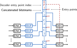
Figure 1: Parallel coding using concatenated independent bitstreams for neural video codecs, with leading decoder entry point index.

However, this only corresponds to the theoretical data entropy. In practice, compressed data must be saved in bitstreams, and in general data elements cannot be randomly accessed for parallel decoding. A simple solution is to split the data to be encoded, and concatenate the resulting variable-length bitstreams, as illustrated in Figure 1.

This requires attaching an entry point index with pointers to the start of each independently coded bitstream. This is a form of bit-rate overhead because the bytes used in this header should be added to compressed data size. A second overhead is with bits “wasted” to finish bitstreams to an integer number of bytes

I-A Paper contributions

We show that, with a number $D$ of compressed data bytes, and $N_{s}<D$ concurrent execution threads, the relative overhead size compared to $D$ is in the form:

$$W(D,N_{s};\alpha,\beta)\approx\frac{N_{s}[\alpha\log_{2}(D/N_{s})+\beta]}{D},$$ (1)

where $\alpha$ and $\beta$ are constants that we show to depend on data organization and index compression. For example, if we simply use $i$ bits for each index element, and have an average of $t$ bits for bitstream termination, we have $\alpha=0$ and $\beta=i+t$.

The objective of this paper is to propose and analyze new schemes to organize data and compress entry points that minimize the relative overhead, or equivalently, minimize factors $\alpha$ and $\beta$, enabling higher parallelization without increasing compression loss.

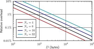
Figure 2: Graph showing an example of how the resulting data overhead depends on the data size $D$ and number of bitstreams $N_{s}$.

Figure 2 shows examples of plots of $W(D,N_{s};\alpha,\beta)$ with values of $\alpha$ and $\beta$ corresponding to another combination of methods (actual parameters and full discussion in Section VI-C). We can observe that since $W(D,N_{s};\alpha,\beta)$ grows with $N_{s}$, we cannot increase parallelization without affecting compression, but we can use the graphs to choose a value of $N_{s}$ such that the relative overhead is acceptably small, which in turn depends on $\alpha$ and $\beta$.

The paper is organized as follows. In Section II we present background material to better define the problem and solutions. The optimization techniques are described in Sections III to V, on using bidirectional bitstream packing, efficiently compressing parallel-decoding entry points, and a new form of jointly optimizing arithmetic coding termination. Experimental results and conclusions are in Sections VI and VII.

II Background

II-A Context-based entropy coding

One of the main problems in the design of multimedia compression is that media signals are far from stationary. Thus, the main technical challenge is not in the process for converting information into bits, which can be done using conventional source coding methods, but in developing statistical data models and effective parameter estimation.

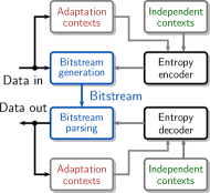
Figure 3: General representation of context-based entropy coding.

Coding contexts are used to represent different data models, and a large number of contexts and codes are commonly used. When considering parallel execution, we can differentiate between adaptation contexts, that depend on the data being coded, and independent contexts that do not, as shown in Figure 3. For generality, we also consider prediction as an adaptation context.

Each component in Figure 3 can be modeled as a finite state machine (FSM), and the whole encoder and decoder by a joint FSM [17]. Bits added to a bitstream depend on both data and encoder state.

The decoder must duplicate the encoder’s sequence of states to correctly parse the bitstream. For that reason, in general it is not possible to simply apply parallel decoders that are set to a pre-defined initial state, to arbitrary parts of the bitstream.

II-B Code self-synchronization

Prefix codes (Golomb-Rice, Huffman, etc.) [18] have relatively simple FSMs, depending on single data inputs. For that reason they may be quickly self-synchronizing, i.e., if decoding starts with an incorrect state, after outputting a few incorrect symbols the decoder probably will recover and start decoding correctly. It has been shown that this property can be exploited for efficient parallel decoding, for example, of JPEG-compressed images [19, 20].

However, it has not been applied to modern video codecs because they use more efficient methods, like arithmetic coding [21, 22, 23] and ANS [24], together with complex context selection, which when combined define FSMs with much larger complexity, exponentially larger state spaces, and thus have much lower probability of self-synchronization.

II-C Parallel coding with independent bitstreams

The simplest form of parallel coding is shown in Figure 1: splitting data and generating independent bitstreams that can be concurrently decoded [25, 26, 17]. The start of each bitstreams is called entry point, because decoders can begin parsing at those positions using pre-defined initial FSM states. Note that, since final sizes of the bitstreams are not known a priori, those bitstreams need to be buffered before their concatenation.

Alternatively, special start markers can be added to the bitstream for identifying decoder entry points, but this requires a more complicated implementation to avoid generating erroneous markers. Other data arrangements are possible when using synchronous vector instructions, but in this paper we assume more scalable asynchronous multithread execution.

This parallelization approach is straightforward, but constrained by compression degradation due to:

(I)

For parallel decoding, adaptation contexts can only use data from the same bitstream, and compression cannot be improved by exploiting dependencies between bitstreams.

(II)

Bits are needed to store an index with the decoding entry point of each independent bitstream.

(III)

There are “wasted” bits in each bitstream, for example, to terminate arithmetic coding, and to generate an integer number of bytes.

II-D Data dependencies and neural-based codecs

Conventional video codecs exploit several types of data dependencies, like intra-frame prediction and entropy coding with adaptive contexts, that need to be disabled or limited for concurrent decoding. This causes fast compression degradation when the number of independent bitstreams increases.

New video compression methods, based on deep-learning and neural networks, can overcome those limitations by changing the way those dependencies are exploited. Figure 4 shows a simplified diagram of an end-to-end neural codec with hyperprior neural networks [12], used in many video codecs [13, 14, 15, 16] (more information about neural codecs can be found in ref. [27]).

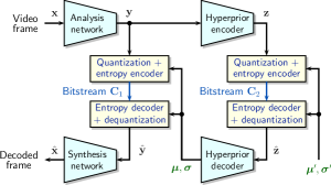
Figure 4: Neural-based codec with hyperprior networks for computing coding parameters.

For our purposes, the important point is that in those codecs the tasks of prediction, bit rate allocation, and distribution estimation, which are commonly done sequentially by conventional codecs, are jointly performed by the hyperprior neural networks shown in the right side of Figure 4.

Those networks generate the parameters ${\boldsymbol{\mu}},{\boldsymbol{\sigma}}$, which are arrays of mean and standard deviation of normal random variables (factorized prior), and define all the parameters needed for coding the image or video data (represented by $\bf y$).

Note that those parameters, in turn, depend on side-information bit stream ${\bf C}_{2}$, which is computed from $\bf y$. What this means is that, to improve compression, neural codecs do exploit data dependencies, but they are computed in a very different manner, amenable to parallel computation and parallel entropy coding.

It is important to note that assumptions like using normal distributions for entropy coding are not observed a posteriori, but are set as design objectives, and practically achieved via deep learning techniques [28, 29].

With this architecture, coding parameters ${\boldsymbol{\mu}},{\boldsymbol{\sigma}}$ define independent contexts (cf. Figure 3), and thus data in $\bf y$ can partitioned and coded in parallel without loss. This eliminates parallelization limitation (I) in the list of Section II-C.

In the next sections we propose methods to minimize factors (II) and (III), and in Section VI-C analyze how their combined use affect overall compression.

III Data organization for parallel coding

In this section we extend a technique that has been used for efficiently arranging two types of compressed data, to many parallel bitstreams as shown in Figure 1. It is used for halving the number of entry points, and thus significantly reduces their index size.

III-A Bidirectional bitstreams

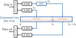
Figure 5: Forward and backward bitstream concatenation for combining arithmetic and binary coded data.

A technique for reducing coding complexity is to decompose data into components that need a more complex method like arithmetic coding, and the remaining data, which is saved directly in their binary representation [30, 31].

It has been observed that, with this scheme, it is not necessary to use extra bits for coding the number bytes used for binary coding if its data is saved in reverse order [32, 33, 34] and the two bitstreams are later concatenated, as shown in Figure 5.

The decoders can pre-load two different types of data at the end of each bitstream, but with appropriate termination (cf. Section V), there are no decoding errors. This is possible because in multimedia compression the number of data symbols to be decoded is known, and the extra data is never parsed [35, §4.1]. It is also easy to avoid invalid memory access by using sufficiently large buffers.

III-B Multiple forward and backward bitstreams

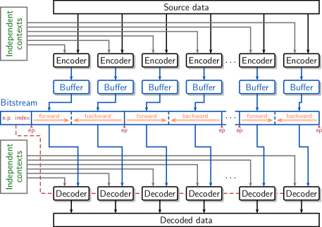
Figure 6: Architecture for parallel entropy coding using entry point index with multiple forward and backward bitstreams.

The compressed data arrangement described in the previous section can be extended to an arbitrary number of bitstream pairs, with the backward stream generated by arithmetic coding. The only changes in the arithmetic decoder implementations is that, after reading a byte, one increments and the other decrements a pointer, which is trivial to implement and does not increase coding complexity.

The combination of those techniques define the parallel entropy coding architecture shown in Figure 6. This approach is more efficient when used with neural codecs because, as explained in Section II-D, they can use only need independent contexts.

In this scheme each entry point defines the position of the first byte in a forward bitstream, and the preceding byte is the first byte of a backward bitstream. Since each position is used for two bitstreams, the total number of entry points is halved. The first and last entry-point are exceptions, but in a compressed video file those positions are respectively at the end and beginning of frames indexes, so we can consider that the total number entry points is halved.

IV Entry point index compression

Assuming $N_{e}$ parallel decoding entry points, as shown in Figure 6, their index is defined by the number of bytes $b_{i}$ in each bitstream $C_{i}$, with entry point positions defined by the cumulative sums

$$h_{0}\equiv 0,\quad h_{n}\stackrel{{\scriptstyle\text{\tiny def}}}{{=}}h_{n-1}+b_{n}=\sum_{i=1}^{n}b_{i},\quad n=1,2,\ldots,N_{e}.$$ (2)

The average and minimum are defined as

$$\bar{b}\stackrel{{\scriptstyle\text{\tiny def}}}{{=}}\frac{1}{N_{e}}\sum_{i=1}^{N_{e}}b_{i},\quad b_{\min}\stackrel{{\scriptstyle\text{\tiny def}}}{{=}}\min\left(b_{1},b_{2},\ldots,b_{N_{e}}\right).$$ (3)

To minimize the index overhead it is necessary to efficiently encode the sequences

$$\mathcal{I}\stackrel{{\scriptstyle\text{\tiny def}}}{{=}}\left(b_{1},b_{2},\ldots,b_{N_{e}}\right),\quad\mbox{or}\quad\mathcal{H}\stackrel{{\scriptstyle\text{\tiny def}}}{{=}}\left(h_{1},h_{2},\ldots,h_{N_{e}}\right).$$ (4)

Theoretically, this is a lossless data compression problem, requiring a statistical model and matched coding method. However, since the index size should be relatively very small, it may be preferable to avoid developing a specialized method for each case.

One alternative, for example, is to simply save each element in $\mathcal{I}$ using the native precision (e.g. 32 bits). This is clearly inefficient, but commonly used because it is trivial to implement. In the next sections we show alternatives that are much more efficient and very simple to implement.

IV-A Universal codes

Even without prior knowledge about $\mathcal{I}$, it is possible to have efficient compression by using “universal” methods, that combine coding with gathering information to improve compression, and that are capable of working well in a wide variety of cases.

Universal prefix codes proposed by Elias [36] are applicable to positive integers. The Elias $\gamma$ or “exp-Golomb” code, is popular and used in video compression standards AVC and HEVC. The number of bits it uses for coding a positive integer number $b$ is

$$E_{\gamma}=2\left\lfloor log_{2}(b)\right\rfloor+1\;\mbox{ bits.}$$ (5)

We can have better compression using a method developed to code all numbers in $\mathcal{I}$ together, like Binary Interpolative Compression (BIC) [37], which can be applied directly to the sequence of entry point positions $\mathcal{H}$, and has an average number of bits equal to

$$R_{\text{bic}}\approx\log_{2}\!\left(\bar{b}\right)+2\;\mbox{ bits/entry point}.$$ (6)

IV-B Range-Tree Compression

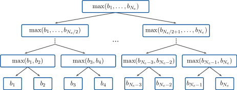
Figure 7: Data used by Range-Tree Compression (RTC).

Figure 8: Concatenations of forward and backward bitstreams with joint arithmetic coding termination.

One limitation of BIC is that it is less efficient when values are tightly grouped around $\bar{b}$, and bit rate (6) becomes much larger than entropy. To cover all cases we propose using the tree-based coding approach of [32] to design a simple universal coding method we call Range-Tree Compression (RTC).

Figure 7 shows the data used by RTC, organized in a binary tree (for convenience we assume $N_{e}$ is a power of two). Managing tree data is simplified when information of a node is stored at position $i$ and information about its descendants is at positions $2i$ and $2i+1$.

Using this convention, we construct arrays with sizes $2N_{e}-1$ and $N_{e}$, containing maximum values and their selection, as

$$a_{i} =\begin{cases}b_{i+1-N_{e}},&N_{e}\leq i\leq 2N_{e}-1,\\ \max(a_{2i},a_{2i+1}),&1\leq i\leq N_{e}-1,\end{cases}$$ (7)

$$x_{i} =\begin{cases}1,&a_{i}=a_{2i},\\ 0,&a_{i}>a_{2i},\end{cases},\quad i=1,2,\ldots,N_{e}.$$ (8)

Note that $\bf a$ is defined from other elements in the same array, but this simply means elements should be computed in reverse order.

With those definitions, we have the following properties

$$a_{2i+1-x_{i}}=a_{i},\quad b_{\min}\leq a_{2i+x_{i}}\leq a_{i}-x_{i}.$$ (9)

which greatly simplify sequentially coding. When the value of $a_{i}$ is known, then we can

1. Use only one bit to code $x_{i}$ and obtain $a_{2i+1-x_{i}}$.

2. Code $a_{2i+x_{i}}$ using a simple method for compressing bounded integers values.

A Python program implementing RTC with few lines of code is provided in the Appendix, and its compression is evaluated in Section VI-A.

V Joint arithmetic coding termination

As mentioned in Section II-C, some extra bits are needed at the end of each bitstreams, and the total overhead increases with the number of bitstreams. In this section we show that, thanks to the bidirectional bitstream organization, arithmetic coding properties can be exploited to reduce the number of termination bits.

V-A Shared arithmetic coding termination bytes

Recent video compression standards and neural-based codecs employ arithmetic coding (AC). Unlike earlier AC versions that process compressed data bits [38, 21, 39], more efficient modern implementations read and write blocks of several bits, commonly 8-bit bytes [40, 41, 22, 23].

When arithmetic encoding finishes, it needs to “flush” pending information and add bits to guarantee correct decoding. The next sections provide more information about this process. Here it suffices to consider that there is a set of valid termination bytes, i.e., values that guarantee correct decoding.

Normally, a single encoder can arbitrarily choose any valid value. With bidirectional bitstreams, on the other hand, we have two encoders, and it is possible to make smarter joint decisions.

Calling $\mathcal{F}$ and $\mathcal{B}$ the sets of valid termination bytes for the forward and backward bitstreams, we have two options when doing concatenation, as shown in Figure 8.

1. If $\mathcal{F}\cap\mathcal{B}=\emptyset$ then set termination bytes to any values $x\in\mathcal{F}$ and $y\in\mathcal{B}$, and concatenate bitstreams.

2. Otherwise, choose any value $z\in\mathcal{F}\cap\mathcal{B}$ for a termination byte that is shared by both bitstreams, saving 8 bits in the resulting concatenated bitstream.

It is interesting to note that nonempty intersections are more probable when there are many values in $\mathcal{F}$ or $\mathcal{B}$, and those correspond to most “wasted” bits, i.e., this technique is most efficient on eliminating the worst cases.

In the next section we discuss how arithmetic coding bitstreams need to be terminated in general, and use those results in Section V-C to define the sets $\mathcal{F}$ and $\mathcal{B}$ shown in Figure 8.

V-B Arithmetic coding termination

Arithmetic coding principles and implementations can be found in several references [38, 21, 39, 41, 22, 23, 26]. In this section we provide only the information required to clarify how sets of valid termination bytes values are defined.

The arithmetic encoder keeps a semi-closed interval (“range” state) defining the fractional number of pending bits. In practice this interval is represented with integers, of precision depending on the implementation.

Figure 9: Factors defining arithmetic coding termination.

We can describe the main principles, applicable to any implementation precision, by defining the encoder’s semi-open final interval $[u,v)$ with real numbers, and normalized such that

$$0\leq u<1,\quad u<v<2,\quad 2^{-8}\leq v-u<1.$$ (10)

In the scheme of Section III-A, the encoder must use termination bits such that, independently of the value of the following bits, the corresponding decoder state is strictly within the final encoder interval, which guarantees correct decoding [35, §5.1.5].

As shown in Figure 9(a), this corresponds to finding an integer $T$ and the minimum integer $s$ that satisfy

$$2^{s}u\leq T<T+1\leq 2^{s}v,\quad T,s\in\mathbb{N}.$$ (11)

Note that at least one extra bit needs to be added since

$$s\geq\left\lceil-\log_{2}(v-u)\right\rceil\geq 1.$$ (12)

When it is possible to choose all the bits in the termination byte, the objective is to instead guarantee correct decoding independently of the following bytes. The corresponding condition is shown in Fig 9(b), where

$$U\stackrel{{\scriptstyle\text{\tiny def}}}{{=}}\left\lceil 2^{8}u\right\rceil\quad V\stackrel{{\scriptstyle\text{\tiny def}}}{{=}}\left\lfloor 2^{8}v\right\rfloor-1.$$ (13)

The condition $V<U$ can occur, but only in some cases when $v-u<2^{-7}$. In those cases an extra renormalization is needed, defining a new interval such that $U<V$. For this reason, in the following discussions we assume that $U\leq V$.

Integers $U$ and $V$ are sufficient to define correct termination, but do not necessarily correspond to final byte values because, following from (10), we can obtain values larger than 255. However, this simply corresponds to one addition carry, which is a normal encoder operation.

For convenience we use the modulo operation to define sets of byte values, with the implicit assumption that the encoder implements the required carry. The set of valid termination bytes is defined by

$$\mathcal{V}(U,V)\stackrel{{\scriptstyle\text{\tiny def}}}{{=}}\{T\bmod 256:U\leq T\leq V,T\in\mathbb{N}\}.$$ (14)

V-C Set intersection and shared termination

Using $U^{(F)}$, $V^{(F)}$, $U^{(B)}$, and $V^{(B)}$ to represent the limits of termination byte values defined in eq. (13), for respectively the forward and backward bitstreams, we have

$$\mathcal{F}=\mathcal{V}\left(U^{(F)},V^{(F)}\right),\quad\mathcal{B}=\mathcal{V}\left(U^{(B)},V^{(B)}\right).$$ (15)

Figure 10 provides an example, where the gray areas represent sets $\mathcal{F}$ and $\mathcal{B}$ and $\mathcal{F}\cap\mathcal{B}$, within the range of byte values [0, 255]. In this example the intersection is not empty, and the shared termination byte can be any integer $z\in[U^{(B)},V^{(F)}-256]$, with a carry operation in the forward bitstream.

Figure 10: Example of sets of valid byte values for terminating arithmetic coding in forward and backward bitstreams.

Note that this form of optimization uses only simple interval intersection determinations, which are computationally very simple, and only needs to be done once before concatenating forward and backward bitstreams.

V-D Reverse bit order

When individual bits are added to the binary bitstream discussed in Section III-A, the termination overhead will be smaller if, in the backward bitstream, both the bytes and bit are written in reverse order.

For arithmetic coding the bit order is defined by the arithmetic operations, but we can still consider what happens when the bit order is reversed before reading and writing backward bitstream bytes (e.g., using table look-up). Defining $\rho(n)$ as the function for bit reversal, we can use the same rules as before, but considering intersection of $\mathcal{F}$ with set

$$\mathcal{B}_{R}=\{\rho(n):n\in\mathcal{B}\}.$$ (16)

In this case set $\mathcal{B}_{R}$ does not contain only intervals, and appear as the multiple gray lines in the example shown in Figure 11, with the dashed red line in the center indicating the line where we can find intersection values that can be shared.

Figure 11: Examples of valid joint termination byte values (gray areas), when the order of bits in the backward bitstream is reversed.

VI Experimental results

VI-A Index compression evaluation

When parallel coding is applied to neural video coding, there are wide variations in the distributions of bitstream sizes, depending on how data is split, quality settings, etc. One expected trend is to have values around a mode (distribution peak), with a longer tail of larger values.

In Figure 12 we have two examples from compressing 100 videos frames from VVC test sequences using the publicly available neural codec by Li et al. [15] and 128 bitstreams/frame, where we can observe a remarkable similarity to a log-normal approximation.

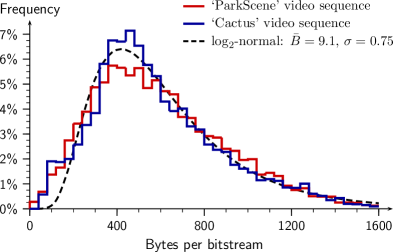
Figure 12: Histograms of bitstream sizes from neural video compression on two video sequences, compared to a $\mbox{\bf log}_{2}$-normal distribution.

Even though universal compression methods are not defined for specific distributions, we can get a good amount of insight by testing them using pseudo-random samples, and in our case from the log-normal probability distribution.

Since the numbers to be coded in $\mathcal{I}$ represent number of bits or bytes, we use a base-2 version of the log-normal distribution, defined from a normal random variable $Z\sim\mathcal{N}(\mu,\,\sigma^{2})$, transformed to generate random variable $B=2^{Z}$, with probability distribution function

$$f_{B}(b;\mu,\sigma)=\frac{1}{b\ln(2)\sigma\sqrt{2\pi}}\,\exp\!\left(\frac{[\log_{2}(b)-\mu]^{2}}{2\sigma^{2}}\right).$$ (17)

Instead of using parameter $\mu$, we use the mean value

$$\bar{B}=2^{\mu+\ln(2)\sigma^{2}/2},$$ (18)

since it corresponds to the expected value of $\bar{b}$, defined in (3). With this notation the source entropy is

$$H_{B}(\bar{B},\sigma)=\log_{2}\!\left(\bar{B}\sigma\ln(2)\sqrt{2e\pi}\right)-\frac{\ln(2)\sigma^{2}}{2}.$$ (19)

TABLE I: Examples of results on neural video compression, 64 bitstreams for parallel decoding, 100 frames (ep = entry point).

Bidir.	Video seq.	BQTerrace				Cactus				ParkScene
	Quality	0	1	2	3	0	1	2	3	0	1	2	3
	$\bar{b}$ (bytes/ep)	100.8	173.2	383.0	816.4	92.0	148.6	269.8	559.0	114.3	188.3	331.7	565.6
	$\log_{2}(\bar{b})+2$	8.7	9.4	10.6	11.7	8.5	9.2	10.1	11.1	8.8	9.6	10.4	11.1
No	$R_{\text{rtc}}$ (bits/ep)	8.1	9.0	10.3	11.4	8.0	8.8	9.8	10.8	8.3	9.2	10.1	10.8
	$\hat{H}$ (bits/ep)	7.9	8.8	9.8	10.3	7.8	8.6	9.3	10.0	8.2	9.0	9.6	10.1
	Overhead $W$ (%)	1.00	0.65	0.34	0.17	1.09	0.74	0.45	0.24	0.91	0.61	0.38	0.24
	$\bar{b}$ (bytes/ep)	201.5	346.3	765.9	1632.7	183.9	297.1	539.5	1117.9	228.3	376.3	663.2	1131.0
	$\log_{2}(\bar{b})+2$	9.7	10.4	11.6	12.7	9.5	10.2	11.1	12.1	9.8	10.6	11.4	12.1
Yes	$R_{\text{rtc}}$ (bits/ep)	9.5	10.4	11.6	12.7	9.5	10.2	11.0	11.8	9.7	10.5	11.2	11.9
	$\hat{H}$ (bits/ep)	9.0	9.8	10.6	11.1	8.9	9.6	10.2	10.8	9.2	9.9	10.5	10.9
	Overhead $W$ (%)	0.59	0.38	0.19	0.10	0.65	0.43	0.25	0.13	0.53	0.35	0.21	0.13

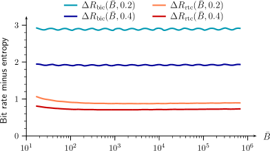
Figure 13: Redundancy of index compression methods applied to samples with $\mbox{\bf log}_{2}$-normal distribution, $\sigma=0.2$ and $\sigma=0.4$, and variable mean $\bar{B}$.

For our experiments on compressing samples from a $\log_{2}$-normal distribution with parameters $\bar{B}$ and $\sigma$, we use $R_{\text{bic}}$ and $R_{\text{rtc}}$ to represent bit rates obtained with BIC and RTC, and the difference between bit rate and source entropy (redundancy) by

$$\Delta R_{\text{bic}}(\bar{B},\sigma) =R_{\text{bic}}-H_{B}(\bar{B},\sigma),$$ (20)

$$\Delta R_{\text{rtc}}(\bar{B},\sigma) =R_{\text{rtc}}-H_{B}(\bar{B},\sigma).$$

Compression methods like BIC and RTC are designed to work well independently of data magnitudes, and the graphs in Figure 13 show that indeed both BIC and RTC—despite not being specifically designed for log-normal distributions—give very consistent results when $\bar{B}$ varies over several orders of magnitude.

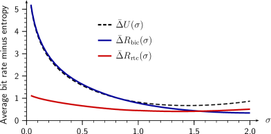
Figure 14: Average redundancies according to standard deviation $\sigma$.

On the other hand, we can also observe that there is are variations caused by $\sigma$, which is what RTC is meant to minimize. Defining the bit rate estimator from eq. (6)

$$\Delta U(\bar{B},\sigma)=\log_{2}\!\left(\bar{B}\right)+2-H_{B}(\bar{B},\sigma),$$ (21)

and using the symbol $\bar{\Delta}$ to represent the average redundancy over the range $4\leq\log_{2}(\bar{B})\leq 20$, we measured its dependency on $\sigma$, and the results are shown in Figure 14.

We can observe that eq. (6) is a good estimator of the BIC bit rates, and how the redundancy quickly grows when $\sigma$ decreases. The proposed RTC method, on the other hand, is more “universal” because its redundancy is nearly independent of the magnitudes and variance.

Table I shows examples of results using the neural codec by Li et al. [15], on VVC test video sequences. For those experiments the tensor with latent variables (data to be compressed) of each frame is “flattened,” and it its data is equally divided for encoding, to generate the $N_{s}$ independent bitstreams.

We can observe that (6) is again a very good estimator of the bit rates, obtained with RTC. In the table we also show $\hat{H}$, representing an estimate of the corresponding source entropy, and roughly $R_{\text{rtc}}<\hat{H}+1.5$.

VI-B Joint termination evaluation

For testing the AC termination described in Section V we used the implementation with 32-bit arithmetic available at the web site from [3] (resources/Software for students^†).

TABLE II: Overhead from byte-based AC termination.

Bidirectional	Reversed	Share	Avrg. extra bits
byte packing	bits	ratio	per bitstream $\bar{T}$
No	—	—	4.56
Yes	No	45%	2.77
Yes	Yes	69%	1.78

Since these tests are only about the AC process, the results are normally independent of the data. Thus, AC termination was tested by coding pseudo-random binary samples with varying probabilities, and results are shown in Table II, where the share ratio represents the fraction of terminations where a byte is shared, as in Figure 8(b).

Thanks to bidirectional byte packing and joint byte termination, and without the more complex reversal of bits in the backward bitstream, in 45% of the cases the final byte can be shared, and the average number of extra bits per bitstream can be reduced from 4.56 to 2.77. With bit reversal the ratio increases to 69% and the average decreases to 1.78 bits.

VI-C Total parallelization overhead

We can combine the previous results to evaluate how they affect the total parallelization overhead, corresponding to eq. (1). We use the following acronyms to represent index formats, and to represent data organization that is combined with optimized AC termination

I32

– entry points represented with 32 bit values.

RTC

– entry points compressed with RTC.

UNI

– unidirectional byte packing.

F+B

– bidirectional byte packing with same bit order within bytes.

F+R

– bidirectional byte packing with reversed bit order in the backward stream.

Eq. (1) results from adding the following overhead terms

• From experimental results in Figure 14 and Table I: when using RTC the average overhead is commonly well-approximated by eq. (6), i.e., $\log_{2}(\bar{b})+2$ per entry point.

• From coding simulations we determined that the average AC termination overhead per bitstream is $\bar{T}$, shown in table II.

With unidirectional byte packing the number of bitstreams is equal to the number of entry point, i.e., $N_{s}=N_{e}$. With bidirectional byte packing we have $N_{s}=2N_{e}$, and given the total number of bytes $D$,

$$\frac{N_{e}[\log_{2}(D/N_{e})+2]+N_{s}\bar{T}}{8D}=\frac{N_{s}[\log_{2}(D/N_{s})+3+2\bar{T}]}{16D}.$$

and with this transformation, and substitution of factors with the obtained numerical values, we obtain the set of factor values $\alpha$ and $\beta$ in eq. (1) shown in Table III. The lines shown in Figure 2 correspond to case F+R & RTC.

Observing that eq. (1) depends only on average bitstream size $\tilde{b}=D/N_{s}$, we can rewrite it as

$$W(\tilde{b};\alpha,\beta)\approx\frac{\alpha\log_{2}(\tilde{b})+\beta}{\tilde{b}},$$ (22)

and plots of this function, using values in Table III, are shown in Figure 15.

TABLE III: Overhead factors for different index coding and data organization.

Order	Index	$\alpha$	$\beta$
UNI	I32	0	4.57
UNI	RTC	1 / 8	0.82
F+B	RTC	1 / 16	0.53
F+R	RTC	1 / 16	0.41

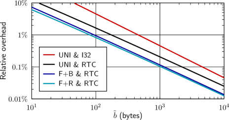
Figure 15: Relative overhead from factors in Table III.

VII Conclusions

As shown in Figure 15, our method significantly reduces the size of the overheads needed for parallel entropy coding. When the average number of bytes per bitstream is sufficiently large, the relative overhead can be small even with an inefficient index format, like I32. In the same figure we can see that the proposed RTC index compression method significantly reduces the overhead.

Despite being extremely simple to implement, it is shown by experimental results in Figs. 13, 14, and Table I, that RTC yields consistently good performance nearly independently of the scales and randomness (measured by entropy).

Employing bidirectional byte packing produces another significant reduction because:

• It halves the number of elements in the entry point index, and as shown by results of Table I, together with RTC consistently yields about 40% index overhead reduction.

• It enables a more efficient form of jointly terminating two arithmetic coding bitstreams, which as shown in Table II, reduce the termination overhead by 40% with simple modifications and 60% with an equally simple, but computationally more expensive AC modification.

-A RTC implementation

This appendix presents a Python implementation of the Range-Tree Compression (RTC) method for coding the array with number of bytes in each bidirectional bitstream, which defines the index of decoder entry points.

The objective is to show that RTC is very simple, requiring only a few lines of Python code. At the same time, as shown by the experimental results, it is quite effective and produces consistently good compression results in a very wide range of situations and data distributions.

We assume that functions pack_bit(x) and unpack_bit(), used for saving and retrieving individual bits to and from a bitstream are already implemented. They are quite simple, and details do not need to be repeated here.

Two other auxiliary functions, pack(n, u) and unpack(u), are used for encoding integer $n$ in a given range defined by $u$, i.e.,

$$n\in\{0,1,2,\ldots,u-1\},$$ (23)

assuming values are equally probable. This can be done with a prefix code [18] that assigns codewords using $\left\lfloor\log_{2}u\right\rfloor$ or $\left\lceil\log_{2}u\right\rceil$ bits. There are many ways to do this, but one of the simplest, which does not require computing $\left\lfloor\log_{2}u\right\rfloor$, is based on a bisection search and is shown below.

⬇

def pack(n, u):

a, b, m = 0, u, u // 2

while a != m:

if n < m: pack_bit(1); b = m

else: pack_bit(0); a = m

m = (a + b) // 2

⬇

def unpack(u):

a, b, m = 0, u, u // 2

while a != m:

if unpack_bit(): b = m

else: a = m

m = (a + b) // 2

return m

Below is the RTC encoder implementation, using the same notation of the paper. The parameters are the number of data elements to be coded N, the array with data b, and an upper bound on all values T. It is assumed N is a power of two.

⬇

def RTC_encode(N, b, T): # encoder function

v, y = [0] * (N * 2), [0] * N # initialization

v[N:2*N] = b[0:N]

b_min = min(b) # computation of b_min

for i in range(N - 1, 0, -1): # and arrays v and y

if v[2*i] >= v[2*i+1]: y[i], v[i] = 1, v[2*i]

else: y[i], v[i] = 0, v[2*i+1]

pack(v[1], T) # encoding v[1] and b_min

pack(b_min, v[1])

for i in range(1, N): # progressive coding of

if v[i] != b_min: # tree-organized data

pack_bit(y[i])

pack(v[i] - v[2*i+y[i]] + y[i] - 1,\

v[i] - b_min + y[i])

This function can be easily optimized, and when N is not a power of two, we can for instance pad the array with b_min.

The corresponding decoder, shown below, does not need two arrays, since it reuses memory initially used for range-tree data to save the final decoded data.

⬇

def RTC_decode(N, T): # decoder function

b = [0] * N # initialization

b[1] = unpack(T) # decoding v[1] and b_min

b_min = unpack(b[1])

for i in range(1, N): # in-place array decoding

j = 2 * i if 2 * i < N else 2 * i - N

b[j] = b[j+1] = b[i]

if b[i] != b_min:

y = unpack_bit()

b[j+y] -= unpack(b[i] - b_min + y) - y + 1

return b # return decoded array

References

- [1] John W. Woods, Multidimensional Signal, Image, and Video Processing and Coding, Academic Press, Waltham, MA, second edition, 2011.
- [2] Thomas Wiegand and Heiko Schwarz, Source Coding: Part I of Fundamentals of Source and Video Coding, now Publishers Inc., Hanover, MA, USA, 2011.
- [3] William A. Pearlman and Amir Said, Digital Signal Compression: Principles and Practice, Cambridge University Press, Cambridge, UK, 2011.
- [4] Vivienne Sze, Madhukar Budagavi, and Gary J. Sullivan, Eds., High Efficiency Video Coding (HEVC): Algorithms and Architectures, Springer International Publishing, Switzerland, 2014.
- [5] Mathias Wien, High Efficiency Video Coding: Coding Tools and Specification, Springer-Verlag, Berlin, 2015.
- [6] John L. Hennessy and David A. Patterson, “A new golden age for computer architecture,” Commun. ACM, vol. 62, no. 2, pp. 48–60, Feb. 2019.
- [7] Krste Asanovic, Ras Bodik, Bryan C. Catanzaro, Joseph J. Gebis, Parry Husbands, Kurt Keutzer, David A. Patterson, William L. Plishker, John Shalf, Samuel W. Williams, and Katherine A. Yelick, “The landscape of parallel computing research: A view from Berkeley,” Tech. Rep. EECS-2006-183, Electrical Engineering and Computer Sciences, University of California, Berkeley, Berkeley, CA, 2006.
- [8] Krste Asanovic, Ras Bodik, James Demmel, Tony Keaveny, Kurt Keutzer, John Kubiatowicz, Nelson Morgan, David A. Patterson, Koushik Sen, John Wawrzynek, David Wessel, and Katherine A. Yelick, “A view of the parallel computing landscape,” Commun. ACM, vol. 52, no. 10, pp. 56–67, Oct. 2008.
- [9] Jie Zhao and Andrew Segall, “Parallel entropy decoding for high resolution video coding,” in Proc. SPIE Vol. 7257: Visual Commun. Image Process., San Jose, CA, Jan. 2009.
- [10] Heiko Schwarz, Thomas Schierl, and Detlev Marpe, “Block Structures and Parallelism Features in HEVC,” in High Efficiency Video Coding (HEVC): Algorithms and Architectures, Vivienne Sze, Madhukar Budagavi, and Gary J. Sullivan, Eds., chapter 3, pp. 49–90. Springer, 2014.
- [11] Valeri George, Jens Brandenburg, Gabriel Hege, Tobias Hinz, Adam Wieckowski, Benjamin Bross, and Detlev Marpe, “Efficient multi-threading strategies in VVenC, an open and optimized VVC encoder implementation,” in Proc. IEEE Int. Symp. Multimedia (ISM), Naples, Italy, Dec. 2022, pp. 18–25.
- [12] Johannes Ballé, David Minnen, Saurabh Singh, Sung Jin Hwang, and Nick Johnston, “Variational image compression with a scale hyperprior,” in Sixth Int. Conf. Learning Representations, Vancouver, Canada, Apr. 2018, arXiv preprint arXiv:1802.01436v2.
- [13] Eirikur Agustsson, David Minnen, Nick Johnston, Johannes Ballé, Sung Jin Hwang, and George Toderici, “Scale-space flow for end-to-end optimized video compression,” in Proc. IEEE/CVF Conf. Comput. Vision Pattern Recognition (CVPR), Seattle, WA, USA, June 2020, pp. 8500–8509, IEEE/CVF.
- [14] Hoang Le, Liang Zhang, Amir Said, Guillaume Sautiere, Yang Yang, Pranav Shrestha, Fei Yin, Reza Pourreza, and Auke Wiggers, “Mobilecodec: neural inter-frame video compression on mobile devices,” in Proc. 13th ACM Multimedia Syst. Conf. (MMSys’22), Athlone, Ireland, June 2022, pp. 324–330, arXiv:2207.08338.
- [15] Jiahao Li, Bin Li, and Yan Lu, “Hybrid spatial-temporal entropy modelling for neural video compression,” in Proc. 30th ACM Int. Conf. Multimedia, Lisboa, Portugal, Oct. 2022, pp. 1503–1511, (code at https://github.com/microsoft/DCVC).
- [16] Jiahao Li, Bin Li, and Yan Lu, “Neural video compression with diverse contexts,” in Proc. Conf. Comput. Vision Pattern Recognition (CVPR), Vancouver, Canada, June 2023, IEEE/CVF, Code at https://github.com/microsoft/DCVC.
- [17] Amir Said, Abo-Talib Mahfoodh, and Sehoon Yea, “Compressed data organization for high throughput parallel entropy coding,” in Proc. SPIE Vol. 9599: Applicat. Digital Image Process., San Diego, CA, USA, Sept. 2015, p. 95991K, SPIE.
- [18] Alistair Moffat, “Huffman coding,” ACM Comput. Surv., vol. 52, no. 4, pp. 85:1–85:35, Aug. 2019.
- [19] Shmuel T. Klein and Yair Wiseman, “Parallel Huffman decoding with applications to JPEG files,” Comput. J., vol. 46, no. 5, pp. 487–497, Jan. 2003.
- [20] André Weißenberger and Bertil Schmidt, “Accelerating JPEG decompression on GPUs,” in Proc. 28th Int. Conf. High Performance Comput. Data Analytics, Bengaluru, India, Dec. 2021, pp. 121–130, arXiv:2111.09219.
- [21] Ian H. Witten, Radford M. Neal, and John G. Cleary, “Arithmetic coding for data compression,” Commun. ACM, vol. 30, no. 6, pp. 520–540, June 1987.
- [22] Amir Said, “Arithmetic coding,” in Lossless Compression Handbook, Khalid Sayood, Ed., chapter 5, pp. 101–152. Academic Press, San Diego, CA, 2003.
- [23] Amir Said, “Introduction to arithmetic coding – theory and practice,” Technical Report HPL-2004-76, Hewlett Packard Laboratories, Palo Alto, CA, USA, Apr. 2004.
- [24] Jarek Duda, Khalid Tahboub, Neeraj J. Gadgil, and Edward J. Delp, “The use of asymmetric numeral systems as an accurate replacement for Huffman coding,” in Proc. Picture Coding Symp., Cairns, Australia, May 2015, IEEE.
- [25] Martin P. Boliek, James D. Allen, Edward L. Schwartz, and Michael J. Gormish, “Very high speed entropy coding,” in Proc. IEEE Int. Conf. Image Process., Austin, TX, USA, Nov. 1994, vol. 3, pp. 625–629.
- [26] Detlev Marpe, Heiko Schwarz, and Thomas Wiegand, “Entropy coding in video compression using probability interval partitioning,” in Proc. Picture Coding Symp., Nagoya, Japan, Dec. 2010, pp. 66–69.
- [27] Siwei Ma, Xinfeng Zhang, Chuanmin Jia, Zhenghui Zhao, Shiqi Wang, and Shanshe Wang, “Image and video compression with neural networks: a review,” IEEE Trans. Circuits Syst. Video Technol., vol. 30, no. 6, pp. 1683–1698, June 2020, arXiv:1904.03567v2.
- [28] Diederik P. Kingma and Max Welling, “Auto-encoding variational Bayes,” in Int. Conf. Learning Representations, Banff, Canada, Apr. 2014, Preprint arXiv:1312.6114v10.
- [29] Ian Goodfellow, Yoshua Bengio, and Aaron Courville, Deep Learning, MIT Press, Cambridge, MA, 2016.
- [30] Detlev Marpe, Heiko Schwarz, and Thomas Wiegand, “Context-based adaptive binary arithmetic coding in the H.264/AVC video compression standard,” IEEE Trans. Circuits Syst. Video Technol., vol. 13, no. 7, pp. 620–636, July 2003.
- [31] Amir Said, “Efficient alphabet partitioning algorithms for low-complexity entropy coding,” in Data Compression Conf., Snowbird, UT, USA, Mar. 2005, pp. 183–192, IEEE.
- [32] Amir Said and William A. Pearlman, “Low-complexity waveform coding via alphabet and sample-set partitioning,” in Proc. SPIE Vol. 3024: Visual Commun. Image Process., San Jose, CA, USA, Feb. 1997, pp. 25–37.
- [33] Jean-Marc Valin, Gregory Maxwell, Timothy B. Terriberry, and Koen Vos, “High-quality, low-delay music coding in the Opus codec,” in Proc. 135th AES Conv., New York, NY, USA, Oct. 2013, Audio Engineering Society, arXiv:1602.04845.
- [34] Antti Hallapuro and Jani Lainema, “Separating context coded and bypass coded data,” Input document JVET-O0450, Joint Video Exploration Team (JVET) of ITU-T SG16 WP3 and ISO/IEC JTC 1/SC29/WG11, Gothenburg, SE, July 2019.
- [35] Jean-Marc Valin, Koen Vos, and Timothy B. Terriberry, “Definition of the Opus Audio Codec,” Tech. Rep. RFC 6716, Internet Engineering Task Force (IETF), Sept. 2012.
- [36] Peter Elias, “Universal codeword sets and representations of the integers,” IEEE Trans. Inf. Theory, vol. 21, no. 2, pp. 194–203, Mar. 1975.
- [37] Alistair Moffat and Lang Stuiver, “Exploiting clustering in inverted file compression,” in Data Compression Conf., Snowbird, UT, USA, Mar. 1996, pp. 82–91, IEEE.
- [38] G. N. N. Martin, “Range encoding: an algorithm for removing redundancy from a digitised message,” in Video and Data Recording Conference, Southampton, UK, July 1979.
- [39] William B. Pennebaker, Joan L. Mitchell, Glen G. Langdon Jr., and Ronald B. Arps, “An overview of the basic principles of the Q-Coder adaptive binary arithmetic coder,” IBM J. Res. Develop., vol. 32, no. 6, pp. 717–726, Nov. 1988.
- [40] Michael Schindler, “A fast renormalisation for arithmetic coding,” in Data Compression Conf., Snowbird, UT, USA, Mar. 1998, p. 572, IEEE.
- [41] Alistair Moffat, Radford M. Neal, and Ian H. Witten, “Arithmetic coding revisited,” ACM Trans. Inf. Syst., vol. 16, no. 3, pp. 256–294, June 1998.
- [42] Ties van Rozendaal, Tushar Singhal, Hoang Le, Guillaume Sautiere, Amir Said, Krishna Buska, Anjuman Raha, Dimitris Kalatzis, Hitarth Mehta, Frank Mayer, Liang Zhang, Markus Nagel, and Auke Wiggers, “MobileNVC: Real-time 1080p neural video compression on a mobiledDevice,” IEEE/CVF Winter Conf. on Applications of Computer Vision (WACV), Jan. 2024.