Extreme Event Prediction with Multi-agent Reinforcement Learning-based Parametrization of Atmospheric and Oceanic Turbulence

Abstract

Global climate models (GCMs) are the main tools for understanding and predicting climate change. However, due to limited numerical resolutions, these models suffer from major structural uncertainties; e.g., they cannot resolve critical processes such as small-scale eddies in atmospheric and oceanic turbulence. Thus, such small-scale processes have to be represented as a function of the resolved scales via closures (parametrization). The accuracy of these closures is particularly important for capturing climate extremes. Traditionally, such closures are based on heuristics and simplifying assumptions about the unresolved physics. Recently, supervised-learned closures, trained offline on high-fidelity data, have been shown to outperform the classical physics-based closures. However, this approach requires a significant amount of high-fidelity training data and can also lead to instabilities. Reinforcement learning is emerging as a potent alternative for developing such closures as it requires only low-order statistics and leads to stable closures. In Scientific Multi-Agent Reinforcement Learning (SMARL) computational elements serve a dual role of discretization points and learning agents. Here, we leverage SMARL and fundamentals of turbulence physics to learn closures for canonical prototypes of atmospheric and oceanic turbulence. The policy is trained using only the enstrophy spectrum, which is nearly invariant and can be estimated from a few high-fidelity samples (these few samples are far from enough for supervised/offline learning). We show that these closures lead to stable low-resolution simulations that, at a fraction of the cost, can reproduce the high-fidelity simulations’ statistics, including the tails of the probability density functions (PDFs). These results demonstrate the high potential of SMARL for closure modeling for GCMs, especially in the regime of scarce data and indirect observations.

1 Introduction

Predicting extreme weather and climate change effects demands simulations that account for complex interactions across nonlinear processes occurring over a wide range of spatiotemporal scales. Turbulence as manifested in atmospheric and oceanic flows, is a prominent example of such nonlinear and multi-scale processes, and plays a critical role in transporting and mixing momentum and heat in the climate system. While the governing equations of turbulent flows are known, GCMs, which are the main tools for predicting climate variability, cannot resolve all the relevant scales. For example, in the atmosphere alone, these scales span from $10^{-4}$ (and smaller) to $10^{4}$ km [1, 2]. Despite advances in our computing capabilities for climate modeling, this limitation is expected to persist for decades.

The effect of unresolved small scales, often referred to as sub-grid scales (SGSs), cannot be ignored in a nonlinear system, and their two-way interactions with the resolved scales have to be accurately accounted for in order for the GCMs to produce stable simulations and the right statistics (climate) and extreme events. Current GCMs use semi-empirical and physics-based representations of SGSs using closures [3]. The input to a closure function is the resolved scales and the output is the SGSs fluxes of momentum, heat, etc. The current closures for many Earth system processes, particularly turbulent flows, fall short of accurately representing the two-way interactions, due to oversimplifications and incomplete theoretical understanding [4, 5]. For example, a major shortcoming is that the current closures are too diffusive (dissipative) and also do not represent a real and important phenomenon called backscattering (basically, anti-diffusion) [6], preventing the GCMs from capturing the extreme events [7, 8]. Recently, there has been growing interest in using machine learning (ML), particularly deep neural networks (DNNs), to learn closures from data. There are two general approaches to ML-based data-driven closure modeling:

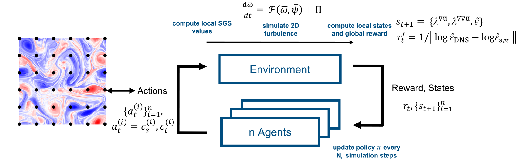
Figure 1: Schematic of training an SGS closure using SMARL. The invariants of gradient and Hessian of velocity ($\lambda^{\nabla\overline{u}}$ and $\lambda^{\nabla\nabla\overline{u}}$) are the states, the actions are the localized (and dynamic) coefficient $c_{s}(x,y,t)$ of classical Smagorinsky or $c_{l}(x,y,t)$ of Leith closures of the SGS term $\Pi(x,y,t)$, and the policy, $\pi$ , learns matching the enstrophy spectrum $\hat{\epsilon}$ to that of the DNS.

Supervised (offline) learning of closures: In this approach, many snapshots of high-fidelity data (e.g., from direct numerical simulation (DNS)) are collected as the “truth”, then filtered and coarse-grained to extract the SGS terms [9]. In turn, these data are used to train a DNN to match the SGS terms $\Pi$ from the closures and from the truth (e.g., using a mean-square-error loss [4]). Once trained, the DNN is coupled to the low-resolution solver to perform large eddy simulation (LES). Studies using a variety of architectures and test cases, from canonical turbulent systems to atmospheric and oceanic flows, have shown the possibility of outperforming classical physics-based closures such as Smagorinsky and Leith [e.g., 4, 8, 10, 11, 12, 13, 14]. However, for many critical climate processes, such high-quality datasets are scarce, extracting the SGS terms is not straightforward, and offline-learned closures can lead to unstable runs [15, 16]. While adding physics to the DNN, transfer learning, and other techniques can address these issues to some degree [14, 17, 18, 19, 20], overall, offline learning remains a promising but challenging approach to data-driven SGS modeling for climate applications.

Online learning of closures: Online learning is emerging as a potent alternative to supervised learning with the closures learned while they operate on the LES. The goal is not to match detailed flow quantities (such as the velocity field or the SGS terms) but instead match the low-order statistics of the high-fidelity simulations or observations. In the context of climate modeling, depending on the application, these statistics could be key properties of climate variability [20] or spectra of turbulent flows [21, 3]. Online learning requires running the numerical model (e.g., a GCM) during the DNN training, which can be challenging. In general, 3 approaches to online learning exists: 1) using a differentiable LES solver/GCM [22, 23, 24], 2) using Ensemble Kalman Inversion (EKI) [25, 26, 27, 20], and 3) using reinforcement learning [28, 29, 30, 31]. While 1-2 have shown promising results, they face major challenges. For example, current GCMs are not differentiable and this approach requires major development in the climate modeling infrastructure [16].

Multi-agent reinforcement learning (MARL), however, has accomplished previously unattainable solutions in ML tasks [e.g., 32, 33, 34], as well as success in improving the parametric and structural uncertainties of closures for 3D homogeneous and wall-bounded turbulent flows [28, 29, 31, 30]. However, its potential in climate-relevant applications, particularly in capturing extreme events, has remained unexplored. Here,

• We train a SMARL-based SGS closure using low-order statistics in climate-relevant flows, i.e., 2D quasi-geostrophic turbulence with different forcing or $\beta$ effects, producing multi-scale jets and vortices like those observed in the Earth’s atmosphere and ocean,

• We remark that we use as input states to the SMARL invariants of the flow and learn the flow-dependent coefficient $c$ of two classic physics-based closures (Leith and Smagorinsky) by matching the enstrophy spectrum the LES solver with that of the DNS (obtained from only 10 true snapshots).

• To test the performance of the data-driven closure, we compare the kinetic energy spectrum and vorticity PDF of the DNS with $160$ to $10240\times$ spatio-temporally coarser LES-MARL. We particularly focus on comparing the tails of these PDFs, as they represent extreme (weather) events in these prototypes. As baselines, we use localized dynamics Smagorinsky and Leith closures, which approximate $c$ as a function of the flow based on physical arguments.

2 Scientific Multi-Agent Reinforcement Learning (SMARL)

In deep-SMARL, a DNN is trained to learn a policy that maps the states to actions. States are fed into a DNN and actions of the agents maximize a reward, see the schematic in Figure 1. Below, we describe the main elements of the training, for which we have utilized Korali, a general-purpose, high-performance framework for deep-SMARL [35].

State:

The state vector consists of a combination of local and global variables. As local states, instantaneous invariants $\lambda$ of filtered velocity gradients [36] and velocity Hessians [28] (5 non-zero local variables) are used. This choice embeds Galilean invariance into the closure. As global states, enstrophy spectrum $\hat{\epsilon}$ is used. We have found the use of these physically motivated invariants, rather than $(\bar{u},\bar{v})$ or $\bar{\psi}$ or their derivatives, to be key in learning successful closures.

Action:

The SGS values at each grid point are required to evolve the governing equations of the environment in time. To retain some degree of interpretability and reduce the computational complexity of training, two classical physics-based closures are employed as the main structure of the SGS closure: (i) Smagorinsky [37], which uses $\nu_{e}=c_{s}\Delta^{2}|\bar{\mathcal{S}}|$, and (ii) Leith [38], which uses $\nu_{e}=c_{l}\Delta^{3}{|\nabla\bar{\omega}|}$, where $\nu_{e}(x,y,t)$ is the eddy viscosity, $\Delta$ is the filter size, $c_{s}(x,y,t)$ and $c_{l}(x,y,t)$ are the key coefficients, and $|\bar{\mathcal{S}}|$, and $|\nabla\bar{\omega}|$ are the magnitudes of the filtered strain rate and $\bar{\omega}$ gradient tensors. The coefficients $c$, which cannot be obtained from first principles, are considered as actions (learned as a function of the state). The actions are interpolated between the agents on to the LES grid via a bilinear scheme, and used to calculate the SGS stress tensor, ${\tau}^{\text{SGS}}=-2\nu_{e}\bar{\mathcal{S}}$, which is then used to compute $\Pi$ that is needed in the low-resolution LES solver, Eq. (1).

Reward:

The goal of our SGS closure is to match a target enstrophy spectrum, which can be calculated from a short-time high-fidelity simulation or few observations. We have computed the spectrum using 10 snapshots from a short DNS run, which is known to be insufficient to learn a successful closer offline in these flows [17]. The reward $r_{t}$ at each time step is defined as the cumulative sum $r_{t}=\Sigma_{s=0}^{t}r^{\prime}_{s}$ of the inverse of the $\mathcal{L}_{2}$ errors of the logarithms of the spectra, i.e., $r^{\prime}_{s}=1/\|\log(\hat{\varepsilon}_{\text{DNS}})-\log(\hat{\varepsilon}_{s,\text{RL}})\|^{2}_{2}$, where $\hat{\varepsilon}_{\text{DNS}}$ is the time-averaged enstrophy spectrum and $\hat{\varepsilon}_{s,\text{RL}}$ is the instantaneous enstrophy spectrum at step $s$. Note that both local variables of the state and the actions are defined at the location of the agents, and agents are uniformly distribution in the domain.

Environment:

The vorticity–streamfunction formulation of the 2D Navier-Stokes equation (NSE) is solved using a pseudo-spectral method. In all cases, $\text{Re}=20000$ and the DNS resolution is $1024$ collocation points in each direction. The solver is coupled with Korali as the environment. Briefly, the environment provides the dynamics of LES given the actions and the states,

$$\frac{\partial\overline{\omega}}{\partial t}=\mathscr{F}(\overline{\omega},\overline{\psi})+\Pi,$$ (1)

where $\Pi(\overline{\psi},\overline{\omega})=\nabla\times(\nabla\cdot\tau^{\text{SGS}})$, $\mathscr{F}(.)$ represents the linear and nonlinear terms of the NSE (see Eq. (2)), and $\overline{\psi}$ and $\overline{\omega}$ are the resolved streamfunction and vorticity on the coarse grid.

3 Experiments

We have developed closures for 3 different forced 2D turbulent flows on the $\beta$-plane (details in Table 1). These cases are commonly used to evaluate the SGS closures of geophysical turbulence [e.g., 39, 17, 13] and exhibit distinct behaviors and dynamics, as seen in snapshots of vorticity fields, $\omega$, in Figure 2. Training is performed with the objective of achieving an LES enstrophy spectrum close to the target (true, DNS) spectrum. We have used the kinetic energy spectra as one unseen test metric. More importantly, the PDFs of the resolved vorticity are compared. The tails of these PDFs represent rare, extreme events, i.e., significantly large $\omega$ with a small probability of occurrence. Note that these vortices resemble the weather system’s high- and low-pressure anomalies, which can cause various extreme weather events [40]. LES with $16$ to $1024\times$ coarser spatial resolution and $10\times$ larger time steps coupled to the learned closures are then ran, and their statistics are compared with those of the DNS and LES with classical dynamic Smagorinsky and Leith closures. As summarized in Figure 2, the tails of the vorticity PDFs clearly show the advantage of the SMARL-based closures, suggesting that these closures have the right amount of diffusion and backscattering (anti-diffusion). The classical closures are too diffusive (a known problem), leading to much less frequent extreme events. The energy spectra also show the better ability of LES with SMARL-based closures in capturing the energy across the scales.

(a) Case 1: $\kappa_{f}=4$, $\beta=0$, $N=32$ ($10240\times$ spatio-temporally coarser)

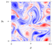
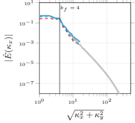
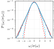
(b) Case 2: $\kappa_{f}=4$, $\beta=20$, $N=32$ ($10240\times$ spatio-temporally coarser)

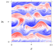
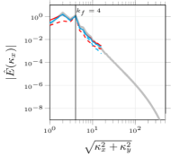
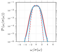
(c) Case 3: $\kappa_{f}=25$, $\beta=0$, $N=256$ ($160\times$ spatio-temporally coarser)

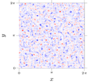
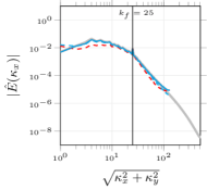
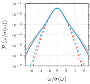
Figure 2: Comparison of LES statistics with SMARL-based closures and the classical closures. Rows (a)-(c) correspond to the cases in Table 1.

4 Conclusion and future work

We have trained a DNN-based SMARL to develop closures for climate-relevant turbulent flows. We show that these closures enable LES with much fewer degrees of freedom than DNS to produce statistics, including energy spectra, PDF, and most importantly, tails of the PDFs, that closely match those of the DNS. Particularly, in terms of capturing extreme events, LES with MARL-based closures significantly outperform LES with classical physics-based closures. The classical closures and even many offline-learned DNNs produce unstable LES unless they are made overly diffusive (e.g., by eliminating backscattering), which comes at the cost of under-representing extreme events [10, 8]. With a small number of samples from DNS, which were not enough to even train an DNN offline [17], SMARL develops closures capable of capturing the statistics of such extreme events, suggesting that both diffusion and backscattering, i.e., the two-way interaction of the resolved scales and SGS, are accurately represented (analysis is in progress to quantify the interscale energy/enstrophy transfers).

Immediate next steps include further analysis and interpretability of the $c$ distributions learned using SMARL and examining the out-of-distribution generalizability of these closures. While offline-learned closures are not expected to extrapolate (e.g., to a different climate) unless methods like transfer learning are used [41], the online-learned closures can be made generalizable by proper scaling of the invariants and spectra [42], which might be possible with enough theoretical understanding of the changing system, e.g., the warming climate [43]. Future work will focus on applying this framework to intermediate-complexity and comprehensive climate models to learn SGS closures (specially for offline-online learning [20]) and systematically calibrate GCMs [44].

Appendix A 2D turbulence

We consider the dimensionless governing equations in the vorticity ($\omega$) and streamfunction ($\psi$) formulation in a doubly periodic square domain with length $L=2\pi$, i.e.,

$$\frac{\partial\omega}{\partial t}+\mathcal{N}(\omega,\psi) = \frac{1}{\text{Re}}\nabla^{2}\omega-f-r\omega+\beta\frac{\partial\psi}{\partial x},$$ (2a)

$$\nabla^{2}\psi = -\omega,$$ (2b)

where $\displaystyle\mathcal{N}(\omega,\psi)=\left(\nicefrac{{\partial\psi}}{{\partial y}}\right)\left(\nicefrac{{\partial\omega}}{{\partial x}}\right)-\left(\nicefrac{{\partial\psi}}{{\partial x}}\right)\left(\nicefrac{{\partial\omega}}{{\partial y}}\right),$ is the nonlinear advection term, and $f(x,y)=\kappa_{f}[\cos{(\kappa_{f}x)}+\cos{(\kappa_{f}y)}]$ is a deterministic forcing [e.g., 45, 46].

To derive the equations for large eddy simulation (LES), we apply sharp spectral filtering [47, 48], denoted by $\overline{(\cdot)}$, to Eq. (2) to obtain

$$\frac{\partial\overline{\omega}}{\partial t}+\mathcal{N}(\overline{\omega},\overline{\psi}) = \frac{1}{\text{Re}}\nabla^{2}\overline{\omega}-\overline{f}-r\overline{\omega}+\beta\frac{\partial\overline{\psi}}{\partial x}+\underbrace{\mathcal{N}(\overline{\omega},\overline{\psi})-\overline{\mathcal{N}({\omega},{\psi})}}_{\Pi=\nabla\times(\nabla\cdot\tau^{\text{SGS}})},$$ (3a)

$$\nabla^{2}\overline{\psi} = -\overline{\omega}.$$ (3b)

The LES is solved on a coarse resolution with the sub-grid scale (SGS) term, $\Pi$, being the unclosed term, requiring a model connecting it to the resolved flow variables, i.e., closure.

For eddy viscosity models:

$${\tau}^{\text{SGS}}=-2\nu_{e}\bar{\mathcal{S}},$$ (4)

where $\mathcal{S}_{ij}=\frac{1}{2}\left(\frac{\partial u_{i}}{\partial x_{j}}+\frac{\partial u_{j}}{\partial x_{i}}\right)$ and $\bar{\mathcal{S}}=\sqrt{2\mathcal{S}_{ij}\mathcal{S}_{ij}}$.

Appendix B Test Cases

The studied cases are summarized in Table 1.

Table 1: The test cases and hyper-parameters in training. $\sigma$ is standard deviation.

Case	Re	$\beta$	$\kappa_{f}$	$r$	$\sigma(\omega)$	$\Delta t_{\text{RL}}/\Delta t_{\text{DNS}}$	Training horizon	Updates policy every
1	$20\times 10^{3}$	$0$	$4$	$0.1$	$5.51$	$10$	$1\times 10^{4}\Delta t_{\text{RL}}$	$10\Delta t_{\text{RL}}$
2	$20\times 10^{3}$	$20$	$4$	$0.1$	$10.75$	$10$	$2\times 10^{4}\Delta t_{\text{RL}}$	$20\Delta t_{\text{RL}}$
3	$20\times 10^{3}$	$0$	$25$	$0.1$	$13.01$	$10$	$1\times 10^{4}\Delta t_{\text{RL}}$	$10\Delta t_{\text{RL}}$

References

- Klein [2010] Rupert Klein. Scale-dependent models for atmospheric flows. Annual Review of Fluid Mechanics, 42(1):249–274, 2010.
- Vallis [2017] Geoffrey K Vallis. Atmospheric and Oceanic Fluid Dynamics. Cambridge University Press, 2017.
- Schneider et al. [2017] Tapio Schneider, Shiwei Lan, Andrew Stuart, and Joao Teixeira. Earth system modeling 2.0: A blueprint for models that learn from observations and targeted high-resolution simulations. Geophysical Research Letters, 44(24):12–396, 2017.
- Rasp et al. [2018] Stephan Rasp, Michael S Pritchard, and Pierre Gentine. Deep learning to represent subgrid processes in climate models. Proceedings of the National Academy of Sciences, 115(39):9684–9689, 2018.
- Hewitt et al. [2020] Helene T Hewitt, Malcolm Roberts, Pierre Mathiot, Arne Biastoch, Ed Blockley, Eric P Chassignet, Baylor Fox-Kemper, Pat Hyder, David P Marshall, Ekaterina Popova, et al. Resolving and parameterising the ocean mesoscale in earth system models. Current Climate Change Reports, pages 1–16, 2020.
- Jansen et al. [2015] Malte F. Jansen, Isaac M. Held, Alistair Adcroft, and Robert Hallberg. Energy budget-based backscatter in an eddy permitting primitive equation model. Ocean Modelling, 94:15–26, 2015. ISSN 1463-5003.
- O’Gorman and Dwyer [2018] Paul A O’Gorman and John G Dwyer. Using machine learning to parameterize moist convection: Potential for modeling of climate, climate change, and extreme events. Journal of Advances in Modeling Earth Systems, 10(10):2548–2563, 2018.
- Guan et al. [2022] Yifei Guan, Ashesh Chattopadhyay, Adam Subel, and Pedram Hassanzadeh. Stable a posteriori LES of 2D turbulence using convolutional neural networks: Backscattering analysis and generalization to higher Re via transfer learning. Journal of Computational Physics, 458:111090, 2022.
- Grooms et al. [2021] Ian Grooms, Nora Loose, Ryan Abernathey, JM Steinberg, Scott Daniel Bachman, Gustavo Marques, Arthur Paul Guillaumin, and Elizabeth Yankovsky. Diffusion-based smoothers for spatial filtering of gridded geophysical data. Journal of Advances in Modeling Earth Systems, 13(9):e2021MS002552, 2021.
- Maulik et al. [2019] Romit Maulik, Omer San, Adil Rasheed, and Prakash Vedula. Subgrid modelling for two-dimensional turbulence using neural networks. Journal of Fluid Mechanics, 858:122–144, 2019.
- Bolton and Zanna [2019] Thomas Bolton and Laure Zanna. Applications of deep learning to ocean data inference and subgrid parameterization. Journal of Advances in Modeling Earth Systems, 11(1):376–399, 2019.
- Yuval and O’Gorman [2020] Janni Yuval and Paul A O’Gorman. Stable machine-learning parameterization of subgrid processes for climate modeling at a range of resolutions. Nature communications, 11(1):3295, 2020.
- Srinivasan et al. [2023] Kaushik Srinivasan, Mickael D. Chekroun, and James C. McWilliams. Turbulence closure with small, local neural networks: Forced two-dimensional and -plane flows. preprint arXiv:2304.05029, 2023.
- Subel et al. [2022] Adam Subel, Yifei Guan, Ashesh Chattopadhyay, and Pedram Hassanzadeh. Explaining the physics of transfer learning a data-driven subgrid-scale closure to a different turbulent flow. arXiv preprint arXiv:2206.03198, 2022.
- Sun et al. [2023] Y Qiang Sun, Pedram Hassanzadeh, M Joan Alexander, and Christopher G Kruse. Quantifying 3d gravity wave drag in a library of tropical convection-permitting simulations for data-driven parameterizations. Journal of Advances in Modeling Earth Systems, 15(5):e2022MS003585, 2023.
- Schneider et al. [2023] Tapio Schneider, Swadhin Behera, Giulio Boccaletti, Clara Deser, Kerry Emanuel, Raffaele Ferrari, L Ruby Leung, Ning Lin, Thomas Müller, Antonio Navarra, et al. Harnessing AI and computing to advance climate modelling and prediction. Nature Climate Change, 13(9):887–889, 2023.
- Guan et al. [2023] Yifei Guan, Adam Subel, Ashesh Chattopadhyay, and Pedram Hassanzadeh. Learning physics-constrained subgrid-scale closures in the small-data regime for stable and accurate LES. Physica D: Nonlinear Phenomena, 443:133568, 2023. ISSN 0167-2789.
- Beucler et al. [2021a] Tom Beucler, Michael Pritchard, Stephan Rasp, Jordan Ott, Pierre Baldi, and Pierre Gentine. Enforcing analytic constraints in neural networks emulating physical systems. Physical Review Letters, 126(9):098302, 2021a.
- Pedersen et al. [2023] Christian Pedersen, Laure Zanna, Joan Bruna, and Pavel Perezhogin. Reliable coarse-grained turbulent simulations through combined offline learning and neural emulation. preprint arXiv:2307.13144, 2023.
- Pahlavan et al. [2023] Hamid A Pahlavan, Pedram Hassanzadeh, and M Joan Alexander. Explainable offline-online training of neural networks for parameterizations: A 1D gravity wave-QBO testbed in the small-data regime. preprint arXiv:2309.09024, 2023.
- Schneider et al. [2021] Tapio Schneider, Andrew M Stuart, and Jin-Long Wu. Learning stochastic closures using ensemble Kalman inversion. Transactions of Mathematics and Its Applications, 5(1):tnab003, 2021.
- Frezat et al. [2022] Hugo Frezat, JL Sommer, Ronan Fablet, Guillaume Balarac, and Redouane Lguensat. A posteriori learning for quasi-geostrophic turbulence parametrization. April, 2(3):6, 2022.
- Shankar et al. [2023] Varun Shankar, Romit Maulik, and Venkatasubramanian Viswanathan. Differentiable turbulence. preprint arXiv:2307.03683, 2023.
- Gelbrecht et al. [2022] M. Gelbrecht, A. White, S. Bathiany, and N. Boers. Differentiable programming for earth system modeling. EGUsphere, 2022:1–17, 2022.
- Kovachki and Stuart [2019] Nikola B Kovachki and Andrew M Stuart. Ensemble kalman inversion: a derivative-free technique for machine learning tasks. Inverse Problems, 35(9):095005, 2019.
- Dunbar et al. [2021] Oliver RA Dunbar, Alfredo Garbuno-Inigo, Tapio Schneider, and Andrew M Stuart. Calibration and uncertainty quantification of convective parameters in an idealized GCM. Journal of Advances in Modeling Earth Systems, 13(9):e2020MS002454, 2021.
- Schneider et al. [2020] Tapio Schneider, Andrew M Stuart, and Jin-Long Wu. Imposing sparsity within ensemble Kalman inversion. arXiv preprint arXiv:2007.06175, 2020.
- Novati et al. [2021a] Guido Novati, Hugues Lascombes de Laroussilhe, and Petros Koumoutsakos. Automating turbulence modelling by multi-agent reinforcement learning. Nature Machine Intelligence, 3(1):87–96, 2021a.
- Kurz et al. [2023] Marius Kurz, Philipp Offenhäuser, and Andrea Beck. Deep reinforcement learning for turbulence modeling in large eddy simulations. International Journal of Heat and Fluid Flow, 99:109094, 2023. ISSN 0142-727X.
- Bae and Koumoutsakos [2022] H Jane Bae and Petros Koumoutsakos. Scientific multi-agent reinforcement learning for wall-models of turbulent flows. Nature Communications, 13(1):1443, 2022.
- Kim et al. [2022] Junhyuk Kim, Hyojin Kim, Jiyeon Kim, and Changhoon Lee. Deep reinforcement learning for large-eddy simulation modeling in wall-bounded turbulence. Physics of Fluids, 34(10), 2022.
- Silver et al. [2017] David Silver, Thomas Hubert, Julian Schrittwieser, Ioannis Antonoglou, Matthew Lai, Arthur Guez, Marc Lanctot, Laurent Sifre, Dharshan Kumaran, Thore Graepel, Timothy P. Lillicrap, Karen Simonyan, and Demis Hassabis. Mastering chess and Shogi by self-play with a general reinforcement learning algorithm. CoRR, abs/1712.01815, 2017.
- Brown and Sandholm [2019] Noam Brown and Tuomas Sandholm. Superhuman AI for multiplayer poker. Science, 365(6456):885–890, 2019. ISSN 0036-8075.
- OpenAI et al. [2019] OpenAI, :, Christopher Berner, Greg Brockman, Brooke Chan, Vicki Cheung, Przemysław Debiak, Christy Dennison, David Farhi, Quirin Fischer, Shariq Hashme, Chris Hesse, Rafal Józefowicz, Scott Gray, Catherine Olsson, Jakub Pachocki, Michael Petrov, Henrique P. d. O. Pinto, Jonathan Raiman, Tim Salimans, Jeremy Schlatter, Jonas Schneider, Szymon Sidor, Ilya Sutskever, Jie Tang, Filip Wolski, and Susan Zhang. Dota 2 with Large Scale Deep Reinforcement Learning. arXiv e-prints, art. arXiv:1912.06680, December 2019.
- Martin et al. [2022] Sergio M. Martin, Daniel Wälchli, Georgios Arampatzis, Athena E. Economides, Petr Karnakov, and Petros Koumoutsakos. Korali: Efficient and scalable software framework for bayesian uncertainty quantification and stochastic optimization. Computer Methods in Applied Mechanics and Engineering, 389:114264, 2022. ISSN 0045-7825.
- Ling et al. [2016] Julia Ling, Andrew Kurzawski, and Jeremy Templeton. Reynolds averaged turbulence modelling using deep neural networks with embedded invariance. Journal of Fluid Mechanics, 807:155–166, 2016.
- Smagorinsky [1963] Joseph Smagorinsky. General circulation experiments with the primitive equations: I. the basic experiment. Monthly Weather Review, 91(3):99 – 164, 1963.
- Leith [1996] C.E. Leith. Stochastic models of chaotic systems. Physica D: Nonlinear Phenomena, 98(2):481–491, 1996. ISSN 0167-2789. Nonlinear Phenomena in Ocean Dynamics.
- Frezat et al. [2021] Hugo Frezat, Guillaume Balarac, Julien Le Sommer, Ronan Fablet, and Redouane Lguensat. Physical invariance in neural networks for subgrid-scale scalar flux modeling. Physical Review Fluids, 6(2):024607, 2021.
- Woollings et al. [2018] Tim Woollings, David Barriopedro, John Methven, Seok-Woo Son, Olivia Martius, Ben Harvey, Jana Sillmann, Anthony R Lupo, and Sonia Seneviratne. Blocking and its response to climate change. Current climate change reports, 4:287–300, 2018.
- Subel et al. [2021] Adam Subel, Ashesh Chattopadhyay, Yifei Guan, and Pedram Hassanzadeh. Data-driven subgrid-scale modeling of forced Burgers turbulence using deep learning with generalization to higher Reynolds numbers via transfer learning. Physics of Fluids, 33(3):031702, 2021.
- Novati et al. [2021b] Guido Novati, Hugues Lascombes de Laroussilhe, and Petros Koumoutsakos. Automating turbulence modelling by multi-agent reinforcement learning. Nature Machine Intelligence, pages 1–10, 2021b.
- Beucler et al. [2021b] Tom Beucler, Michael Pritchard, Janni Yuval, Ankitesh Gupta, Liran Peng, Stephan Rasp, Fiaz Ahmed, Paul A O’Gorman, J David Neelin, Nicholas J Lutsko, et al. Climate-invariant machine learning. arXiv preprint arXiv:2112.08440, 2021b.
- Balaji et al. [2022] V Balaji, Fleur Couvreux, Julie Deshayes, Jacques Gautrais, Frédéric Hourdin, and Catherine Rio. Are general circulation models obsolete? Proceedings of the National Academy of Sciences, 119(47):e2202075119, 2022.
- Chandler and Kerswell [2013] Gary J Chandler and Rich R Kerswell. Invariant recurrent solutions embedded in a turbulent two-dimensional Kolmogorov flow. Journal of Fluid Mechanics, 722:554–595, 2013.
- Kochkov et al. [2021] Dmitrii Kochkov, Jamie A Smith, Ayya Alieva, Qing Wang, Michael P Brenner, and Stephan Hoyer. Machine learning–accelerated computational fluid dynamics. Proceedings of the National Academy of Sciences, 118(21), 2021.
- Pope [2001] Stephen B Pope. Turbulent Flows. IOP Publishing, 2001.
- Sagaut [2006] Pierre Sagaut. Large eddy simulation for incompressible flows: An introduction. Springer Science & Business Media, 2006.