Nash Learning from Human Feedback

Abstract

Reinforcement learning from human feedback (RLHF) has emerged as the main paradigm for aligning large language models (LLMs) with human preferences. Typically, RLHF involves the initial step of learning a reward model from human feedback, often expressed as preferences between pairs of text generations produced by a pre-trained LLM. Subsequently, the LLM’s policy is fine-tuned by optimizing it to maximize the reward model through a reinforcement learning algorithm. However, an inherent limitation of current reward models is their inability to fully represent the richness of human preferences and their dependency on the sampling distribution.
In this study, we introduce an alternative pipeline for the fine-tuning of LLMs using pairwise human feedback. Our approach entails the initial learning of a preference model, which is conditioned on two inputs given a prompt, followed by the pursuit of a policy that consistently generates responses preferred over those generated by any competing policy, thus defining the Nash equilibrium of this preference model. We term this approach Nash learning from human feedback (NLHF).  In the context of a tabular policy representation, we present a novel algorithmic solution, Nash-MD, founded on the principles of mirror descent. This algorithm produces a sequence of policies, with the last iteration converging to the regularized Nash equilibrium. Additionally, we explore parametric representations of policies and introduce gradient descent algorithms for deep-learning architectures. To demonstrate the effectiveness of our approach, we present experimental results involving the fine-tuning of a LLM for a text summarization task. We believe NLHF offers a compelling avenue for preference learning and policy optimization with the potential of advancing the field of aligning LLMs with human preferences.

1 Introduction

Large language models (LLMs) (Glaese et al., 2022; Anil et al., 2023; OpenAI, 2023; Ouyang et al., 2022) have made remarkable strides in enhancing natural language understanding and generation. Their success in conversational applications often relies on aligning these models with human preferences, a process primarily guided by the paradigm of reinforcement learning from human feedback (RLHF). A prevailing approach within RLHF involves the initial step of constructing a reward model based on pairwise human preferences, frequently employing the Bradley-Terry model (BT; Bradley and Terry, 1952). This reward model assigns an individual score to each generation of the language model conditioned on a given prompt, akin to how the Elo (1978) ranking system assigns scores to chess players to estimate their relative strengths. Subsequently, model refinement takes place by optimizing the LLM’s performance with respect to this reward model through reinforcement learning (RL) over sampled text generations.

However, the Elo model has its limitations, primarily coming from its inability to accommodate the full spectrum of possible preferences. For example, Bertrand et al. (2023) show the limitations of the Elo model by illustrating where Elo score alone cannot predict the right preferences, even in transitive situations. There are also situations where maximizing the Elo score is not aligned with maximizing the probability of winning against the relevant population of players, even when the preference model can be perfectly expressed using a BT model (see Appendix A for an example). These observations highlight the necessity for a more profound understanding of the implications of Elo-based reward maximization in RLHF for achieving genuine alignment with human preferences.

In this paper, we introduce an alternative pipeline for fine-tuning LLMs from human preference data, which we term Nash learning from human feedback (NLHF). In this framework, we depart from the conventional approach of learning a reward model and instead focus on learning a preference model and define our objective to compute the Nash equilibrium of this preference model.

The preference model takes two responses, denoted as $y$ and $y^{\prime}$ (possibly conditioned on a prompt $x$), as input and produces a preference score ${\cal{P}}(y\succ y^{\prime}|x)$, indicating the preference of response $y$ over response $y^{\prime}$ given the context $x$. To initialize this preference model, we may leverage an LLM prompted in a manner akin to how humans have been asked for their preference, such as by instructing the LLM to generate a 1-vs-2 comparison in response to a prompt like: “Given $x$, which answer do you prefer, answer 1: $y$ or answer 2: $y^{\prime}$?”. This initial preference model can be further refined through supervised learning to align it with human preference data. Notably, a preference model does not require the assumption of the Bradley-Terry model, and thus has the potential to capture a more diverse range of human preferences. Moreover, in contrast to the traditional RLHF setting where the reward model depends on the distribution (and thus the policy) of responses used to collect human data, a preference model (having as input the two responses to be compared) remains essentially invariant to the specific policy employed to generate these responses. Finally, we argue (below) that the Nash equilibrium of the preference model is a solution that better aligns with the diversity of human preferences than the maximum of the expected reward model.

Once the preference model is established, our primary objective is to calculate the corresponding Nash equilibrium. This equilibrium represents a policy that consistently produces responses preferred, as determined by the preference model, over responses generated by any alternative policy. The beauty of this solution concept lies in its innate alignment with the human preference data that served as the foundation for training the preference model. These three key properties of our approach, namely, the ability of the preference model to encompass a wider spectrum of human preferences, its policy-independence, and the potential for the Nash equilibrium to provide a better alignment with the diversity of human preferences, mark a substantial departure from the conventional RLHF framework. We discuss these properties in greater detail in Section 3.

To approximate the Nash equilibrium of the two-player game in which actions are responses, and payoffs are specified by the preference model, we employ a deep reinforcement learning algorithm. Given a prompt $x$, we generate two responses, denoted as $y$ and $y^{\prime}$. The first response, $y$, is generated under the current policy $\pi_{\theta}$ that we are in the process of optimizing. In contrast, the second response, $y^{\prime}$, is produced by an alternative policy $\pi^{\prime}$, which we implement in two different versions: Nash-MD and Nash-EMA (further elaboration on these versions will be provided below). Nash-MD defines the alternative policy $\pi^{\prime}$ as a geometric mixture between the initial and the current policies (motivated by mirror descent), whereas Nash-EMA implements a first-order approximation of an exponential moving average (EMA) mixture of past policies. Then, the preference model computes ${\cal{P}}(y\succ y^{\prime}|x)$, and this preference signal serves as a reward for optimizing our policy $\pi_{\theta}$ using a (regularized) policy gradient algorithm, as outlined by Geist et al. (2019).

Our contributions in this work can be summarized as follows. First, we introduce the concept of Nash learning from human feedback (NLHF), framing it as the task of computing the Nash equilibrium for a general preference model. We proceed by introducing and defining a regularized variant of the preference model. We also establish the existence and uniqueness of the corresponding Nash equilibrium in this context. Then, we consider the case of tabular policy representations and introduce a novel algorithm named Nash-MD. This algorithm, founded on the principles of mirror descent (MD) possesses two important properties. First, it converges to the Nash equilibrium, with the final iteration reaching this equilibrium. This differs from conventional regret-minimization-based algorithms, where it is typically the mixture of past policies that converges, necessitating the storage of past policies. Secondly, Nash-MD learns by competing against alternative policies $\pi^{\prime}$ that represent a (geometric) mixture between the current policy $\pi_{\theta}$ and the initial policy. Importantly, this can be accomplished without the need to retain intermediate policies, a feature of particular significance in the context of LLMs with their substantial memory requirements. Additionally, we introduce Nash-EMA, a variation inspired by fictitious play, which uses an exponential moving average of past policy parameters. We introduce policy-gradient algorithms for deep learning architectures, Nash-MD-PG and Nash-EMA-PG, inspired by the tabular algorithms Nash-MD and Nash-EMA. We present the results of extensive numerical experiments conducted on a text summarizing task utilizing the TL;DR dataset (Völske et al., 2017). In these experiments, we employ the NLHF approach to train several models. To assess their performance, we conduct a pairwise evaluation (using the PaLM 2 Large LLM) of the performance of the models and include a comparison to an RLHF baseline. We conclude that NLHF opens up new promising directions for aligning LLMs with human preferences.

2 Prior work

Preference-based RL.

Our contribution falls into a broader area of preference-based RL, where we directly learn from pairwise human preferences instead of a hand-designed or learned scalar reward (see, e.g., the survey by Wirth et al., 2017). The canonical form of RLHF was proposed in Christiano et al. (2017) and popularized by OpenAI (2022), in which one learns a scalar reward model from the preference feedback, followed by policy optimization against the reward model. However, an advantage of directly optimizing for preferences rather than a learnt scalar reward function is the potential to avoid reward hacking (Amodei et al., 2016), when agents find a way to maximize a reward without performing what was intended. Furthermore, in domains such as medical applications, it may not only be challenging but also undesirable to provide a single scalar reward.

In general, the preference feedback can be provided in different ways, e.g., on the level of states, actions, or a full trajectory. In this work, we focus on the trajectory feedback where the experts provide feedback by selecting the preferred one of the two proposed trajectories. Such a simple form of pairwise feedback is the easiest to implement, and has seen applications in summarization  (Stiennon et al., 2020), question-answering (Nakano et al., 2021; Menick et al., 2022) and general language-based assistants (Ouyang et al., 2022; Glaese et al., 2022; Bai et al., 2022). More complicated forms of feedback has been studied in theoretical literature such as Efroni et al. (2021).

Theoretical guarantees for learning from preferences.

Learning policies from preference feedback of histories was studied by Akrour et al. (2011) who learned the preference model for histories and by Cheng et al. (2011) who trained a model ranking actions for a state. Busa-Fekete et al. (2014, 2013) approached this setting by comparing and ranking policies and Wilson et al. (2012) by learning a distribution over policy space. Preference-based RL is also explored in dueling RL (Novoseller et al., 2020; Pacchiano et al., 2023), which generalizes the well-studied dueling bandits problem. In particular, Pacchiano et al. (2023) assumes a Bradley-Terry model, which they estimate using maximum likelihood in the tabular setting.

Our work is also related to results of Wang et al. (2023) who consider learning Nash equilibria of the human preference model, and reduce the problem to finding Nash equilibria for a special class of factored two-player Markov games under a restricted set of policies. Moreover, Chen et al. (2022) gave first results for function approximation in preference-based RL, however with a computationally inefficient algorithm.

Optimization without reward function.

A number of recent works has attempted to optimize for preference feedback without learning a reward function. For example, Direct Preference Optimization (DPO; Rafailov et al., 2023) optimizes the policy through a loss function defined via the Bradley-Terry reward model. SLiC-HF (Zhao et al., 2023) modifies the classical RLHF training loss by calibrating a ranking loss which contrasts a positive and a negative sequence. This resembles directly optimizing for the pairwise preference, albeit without convergence guarantees. Identity Policy Optimization (IPO; Azar et al., 2023) proposed to directly optimize the pairwise human preference with offline preference data. Unlike DPO, IPO does not make the assumption on reward model, though they both optimize against a fixed opponent rather than searching for Nash equilibria.

3 The preference model and its Nash equilibrium

We now introduce the core conceptual ideas behind our approach to learning from preference feedback. We consider a preference model in a contextual bandit setting. Given a context (or prompt) $x$ in the context space $\mathcal{X}$ and two actions (or responses/choices) $y$ and $y^{\prime}$ in the action space $\mathcal{Y}$, the preference of $y$ over $y^{\prime}$ is a number between $0$ and $1$ which is written ${\cal P}(y\succ y^{\prime}|x)$. We will assume that the preference model is symmetric: ${\cal{P}}(y\succ y^{\prime}|x)=1-{\cal{P}}(y^{\prime}\succ y|x)$.

An example of such a preference model is the probability (under some random outcome $Z$) that $f(x,y,Z)\geq f(x,y^{\prime},Z)$, where $f$ is a (deterministic) absolute scoring function:

$${\cal P}(y\succ y^{\prime}|x)=\mathbb{E}_{Z\sim\nu}\left[\mathbb{1}\{f(x,y,Z)\succ f(x,y^{\prime},Z)\}\right],$$

where we define the function $\mathbb{1}\{u\succ v\}\stackrel{{\scriptstyle\rm def}}{{=}}(\operatorname{sign}(u-v)+1)/2$, which behaves as an indicator for the event $u>v$, and assigning a value of $1/2$ in the case where $u=v$. For example, this could represent the probability that a randomly chosen human $Z\sim\nu$ prefers choice $y$ over choice $y^{\prime}$ in a context $x$. We assume that we do not have access to the absolute human scores $f$ but only to their relative preferences.

We define the preference between two distributions conditioned on a state $x$:

$${\cal P}(\pi\succ\pi^{\prime}|x)\stackrel{{\scriptstyle\rm def}}{{=}}\mathbb{E}_{y\sim\pi(\cdot|x),y^{\prime}\sim\pi^{\prime}(\cdot|x)}\left[{\cal{P}}(y\succ y^{\prime}|x)\right]$$

and the preference of an action over a distribution ${\cal P}(y\succ\pi^{\prime}|x)\stackrel{{\scriptstyle\rm def}}{{=}}\mathbb{E}_{y^{\prime}\sim\pi^{\prime}(\cdot|x)}\left[{\cal{P}}(y\succ y^{\prime}|x)\right]$. Finally, given a distribution $\rho$ over contexts, we define the preference between two policies:

$${\cal P}(\pi\succ\pi^{\prime})\stackrel{{\scriptstyle\rm def}}{{=}}\mathbb{E}_{x\sim\rho}\mathbb{E}_{y\sim\pi(\cdot|x),y^{\prime}\sim\pi^{\prime}(\cdot|x)}\left[{\cal{P}}(y\succ y^{\prime}|x)\right].$$

We say that a policy $\pi$ is preferred over (or simply wins against) another policy $\pi^{\prime}$ if ${\cal P}(\pi\succ\pi^{\prime})\geq 1/2$. In the remainder of the paper, we assume without loss of generality that $\rho$ assigns every context positive probability.

In this paper we will consider the objective of finding a policy $\pi^{*}$ which is preferred over any other alternative policy:

$$\pi^{*}\stackrel{{\scriptstyle\rm def}}{{=}}\arg\max_{\pi}\min_{\pi^{\prime}}{\cal P}(\pi\succ\pi^{\prime})\,.$$ (1)

This objective implicitly defines a two-player game, in which the players select policies $\pi$ and $\pi^{\prime}$, the first player receiving a payoff of ${\cal P}(\pi\succ\pi^{\prime})$, and the second player receiving ${\cal P}(\pi^{\prime}\succ\pi)=1-{\cal P}(\pi\succ\pi^{\prime})$. This is therefore a two-player, symmetric, constant-sum game, and it follows that when both players use a policy $\pi^{*}$ solving Equation (1), this is a Nash equilibrium for this game, by the minimax theorem (von Neumann, 1928). This is the fundamental solution concept we study in this paper.

The objective introduced in Equation (1) has two central differences relative to the majority of existing work on RLHF. First, the objective is expressed directly in terms of preferences themselves, not in terms of a reward function learnt from preferences, and also not in terms of a non-linear transformation of the preferences. Second, our solution concept relies on the notion of Nash equilibrium, rather than on optimization against a fixed behavior. We discuss the impact of both of these choices through several examples below.

3.1 Limited expressivity of reward models

Notice that in general the preference model may not be transitive and we can have 3 policies $\pi_{1}$, $\pi_{2}$ and $\pi_{3}$ such that ${\cal{P}}(\pi_{1}\succ\pi_{2})>1/2$, ${\cal{P}}(\pi_{2}\succ\pi_{3})>1/2$ and ${\cal{P}}(\pi_{3}\succ\pi_{1})>1/2$. For example, consider the set of outcomes being the subset of integers $\mathcal{Y}=\{1,2,\dots,9\}$ and 3 policies defined by $\pi_{1}={\cal U}(\{2,4,9\})$, $\pi_{2}={\cal U}(\{1,6,8\})$, and $\pi_{3}={\cal U}(\{3,5,7\})$, where ${\cal U}(S)$ refers to a uniform distribution over the set $S$. The preference is defined as ${\cal P}(\pi\succ\pi^{\prime})=\mathbb{E}_{y\sim\pi,y^{\prime}\sim\pi^{\prime}}[\mathbb{1}\{y\geq y^{\prime}\}]$. Then we have ${\cal P}(\pi_{1}\succ\pi_{2})={\cal P}(\pi_{2}\succ\pi_{3})={\cal P}(\pi_{3}\succ\pi_{1})=5/9$. This mirrors the classical example of non-transitive dice (Gardner, 1970).

Preference models, as demonstrated, possess the capacity to encompass non-transitive preferences, a characteristic not attainable by reward models, which inherently assign a single score to each policy. Whether humans exhibit non-transitive preferences or not has been a subject of longstanding research (see, for instance, Tversky 1969; Klimenko 2015). Additionally, non-transitivity is not the only limitation of Bradley-Terry-based reward models; see, e.g., Example 3 in Bertrand et al. (2023) where Elo score fails to capture the correct preference ordering between policies, even in transitive situations. In fact, we show in Appendix A that even when the preference model is perfectly captured by the Bradley-Terry model, optimization of the reward/Elo score may still disagree with any reasonable notion of preference optimization. Therefore, we can safely argue that preference models offer a more flexible and nuanced framework for modeling human preferences than reward models.

3.2 Alignment with diversity of human preferences

Here, we illustrate that in some situations, the solution offered by the Nash equilibrium of the preference model (which we refer to as the NLHF solution) is more aligned with the diversity of human preferences than the optimum of the reward model (which we refer to as the RLHF solution).

Consider the following situation where there are 3 different actions ($y_{1}$, $y_{2}$, $y_{3}$) and we have a population composed of 3 types of humans with respective preferences ${\cal{P}}_{1},{\cal{P}}_{2},{\cal{P}}_{3}$, defined in the following way: ${\cal{P}}_{i}(y_{1}\succ y_{2})={\cal{P}}_{i}(y_{1}\succ y_{3})={\cal{P}}_{i}(y_{2}\succ y_{3})=1/2$, for $1\leq i\leq 3$, except for the following cases: ${\cal{P}}_{1}(y_{2}\succ y_{1})=1$ (thus ${\cal{P}}_{1}(y_{1}\succ y_{2})=0$), ${\cal{P}}_{2}(y_{1}\succ y_{3})=1$ (thus ${\cal{P}}_{2}(y_{3}\succ y_{1})=0$), and ${\cal{P}}_{3}(y_{3}\succ y_{2})=1$ (thus ${\cal{P}}_{3}(y_{2}\succ y_{3})=0$).

Now, let us assume these 3 types form a near-uniform distribution over humans, for example ${\mathbb{P}}(\mbox{Type }1)=1/3-\epsilon$, ${\mathbb{P}}(\mbox{Type }2)={\mathbb{P}}(\mbox{Type }3)=1/3+\epsilon/2$. The corresponding population preference is thus ${\cal{P}}_{\epsilon}=(1/3-\epsilon){\cal{P}}_{1}+(1/3+\epsilon/2)({\cal{P}}_{2}+{\cal{P}}_{3})$. In the case $\epsilon>0$ (so Type 1 is slightly less frequent than the other types) then a reward model will assign a slightly better reward (assuming a Bradley-Terry model) to action $y_{1}$, thus optimizing the expected reward (the RLHF solution) will produce a deterministic policy choosing exclusively $y_{1}$.

However, here we are in a situation where the preferences are not uniformly aligned across humans. In the case of uniform sampling of humans (i.e., $\epsilon=0$), the Nash equilibrium of ${\cal{P}}_{\epsilon=0}$ is a uniform mixture between the 3 policies. Actually, the preference model ${\cal{P}}_{\epsilon}$ corresponding to any $\epsilon$ is defined as: ${\cal{P}}_{\epsilon}(y_{2}\succ y_{1})=2/3-\epsilon/2$, ${\cal{P}}_{\epsilon}(y_{3}\succ y_{1})=1/3-\epsilon/4$, ${\cal{P}}_{\epsilon}(y_{3}\succ y_{2})=2/3+\epsilon/4$, ${\cal{P}}_{\epsilon}(y_{i}\succ y_{i})=1/2$, and ${\cal{P}}_{\epsilon}(y_{i}\succ y_{j})=1-{\cal{P}}_{\epsilon}(y_{j}\succ y_{i})$, for $1\leq i<j\leq 3$. By a simple calculation, we deduce that for any $|\epsilon|\leq 1/3$, the Nash equilibrium of this preference model consists in selecting $y_{1}$ and $y_{2}$ with probability $1/3+\epsilon/2$ each, and $y_{3}$ with probability $1/3-\epsilon$.

We believe that in this situation, the Nash solution of the preference model (i.e., the NLHF solution), assigning close to uniform probability to these 3 actions (one being preferred by each category of humans) is more aligned with the diversity of human preferences than the optimum of the reward model (i.e., the RLHF solution), which would deterministically select a single action. Also the Nash equilibrium is less sensitive to the preference distribution, since the corresponding equilibrium is smooth w.r.t. change in the distribution over types of humans (i.e., when $\epsilon$ varies near $0$), whereas the RLHF solution will switch from selecting exclusively $y_{1}$ when $\epsilon>0$ to selecting exclusively $y_{2}$ when $\epsilon<0$.

3.3 Sensitivity to the sampling distribution

Another difference between reward and preference models is that a reward model depends on the distribution over responses it has been trained on, whereas a preference model essentially does not. Indeed, when we learn a reward model we are solving the following optimization problem:

$$r^{\pi}\stackrel{{\scriptstyle\rm def}}{{=}}\arg\max_{r(\cdot,\cdot)}\mathbb{E}_{x\sim\rho,y,y^{\prime}\sim\pi(\cdot|x),Z\sim\nu}\mathbb{E}\left[\log\left(\sigma(r(x,y_{w}^{h})-r(x,y_{l}^{h}))\right)\right],$$

where $y_{w}^{h}$ and $y_{l}^{h}$ are respectively the preferred (and less preferred) response (among $y$ and $y^{\prime}$) according to a randomly sampled human $Z\sim\nu$, given $x$. The (optimal) solution to this problem $r^{\pi}$ depends on the policy $\pi$ that has generated the data. Indeed, as mentioned in the introduction (see Section 1), the reward model assigns an Elo score to each individual response, which is defined in terms of a comparison against other responses; thus, it depends on the overall distribution over responses it has been trained on.

On the contrary, since the preference model takes two responses as input, the output does not depend directly on the distribution these responses have been sampled from. The preference model is simply learnt by supervised learning, where for each $x,y,y^{\prime}$, the preference model ${\cal{P}}(y\succ y^{\prime}|x)$ is regressed to the human preference $\mathbb{1}\{y\mbox{ is preferred to }y^{\prime}\mbox{ given }x\}$ using a cross entropy loss:

$${\cal{P}}^{*}\stackrel{{\scriptstyle\rm def}}{{=}}\arg\max_{{\cal{P}}(\cdot\succ\cdot|\cdot)}\mathbb{E}_{x\sim\rho,y\sim\pi(\cdot|x),y^{\prime}\sim\pi^{\prime}(\cdot|x),Z\sim\nu}\mathbb{E}\left[\log{\cal{P}}(y_{w}^{h}\succ y_{l}^{h}|x)\right].$$

Notice that the optimal solution to this optimization problem is, for every $x\in\mbox{supp}(\rho)$, $y\in\mbox{supp}(\pi(\cdot|x))$, $y^{\prime}\in\mbox{supp}(\pi^{\prime}(\cdot|x))$,

$${\cal{P}}^{*}(y\succ y^{\prime}|x)={\mathbb{P}}_{Z\sim\nu}\left(\mbox{Human }Z\mbox{ prefers }y\mbox{ to }y^{\prime}\mbox{ given }x\right),$$

thus does not depend on $\rho$, $\pi$ or $\pi^{\prime}$. Now, of course, when using approximate models the learned preference model may still depend on the data distribution as the quality of the approximate model will depend on the local quantity of data collected.

Thus it is our general expectation that the preference model is significantly less reliant on the specific policy that generated the data when compared to the reward model.

This observation becomes even more important in scenarios where multiple iterations of RLHF/NLHF occur, comprising data collection, constructing a reward/preference model, policy optimization based on the model, and collecting new data following the updated policy.

In the case of RLHF, the reward model from a prior iteration diverges from the next iteration due to shifts in data generation, necessitating complete relearning. On the contrary, in the NLHF approach, the preference model can be preserved and further enriched through the introduction of novel data, thereby offering a more seamless and efficient adaptation process.

4 Regularized preference model

We now consider a regularized version of the preference model. This is motivated by situations where the preference model is more accurately estimated when following some given policy. This could include the policy responsible for generating the data used to train the preference model or situations where it is imperative to ensure that our solution remains close to a known safe policy. In such cases, we incorporate a penalty mechanism into our preference model, employing KL-regularization to quantify the divergence between the policy under consideration and a designated reference policy denoted as $\mu$; see Jaques et al. (2019); Stiennon et al. (2020); Ouyang et al. (2022) for further details on the role KL-regularization in RLHF.

The regularized preference between actions $y\sim\pi(\cdot|x),y^{\prime}\sim\pi^{\prime}(\cdot|x)$ is defined as

$${\cal P}_{\tau}^{\pi,\pi^{\prime}}(y\succ y^{\prime}|x)\stackrel{{\scriptstyle\rm def}}{{=}}{\cal P}(y\succ y^{\prime}|x)-\tau\log\frac{\pi(y|x)}{\mu(y|x)}+\tau\log\frac{\pi^{\prime}(y^{\prime}|x)}{\mu(y^{\prime}|x)},$$

and we define accordingly the KL-regularized preference between policies:

$${\cal P}_{\tau}(\pi\succ\pi^{\prime}) \stackrel{{\scriptstyle\rm def}}{{=}} \mathbb{E}_{x\sim\rho,y\sim\pi(\cdot|x),y^{\prime}\sim\pi^{\prime}(\cdot|x)}\left[{\cal P}_{\tau}^{\pi,\pi^{\prime}}(y\succ y^{\prime}|x)\right]$$ (2)

$$= {\cal P}(\pi\succ\pi^{\prime})-\tau\mbox{KL}_{\rho}(\pi,\mu)+\tau\mbox{KL}_{\rho}(\pi^{\prime},\mu),$$

where $\mbox{KL}_{\rho}(\pi,\mu)=\mathbb{E}_{x\sim\rho}[\mbox{KL}(\pi(\cdot|x),\mu(\cdot|x))]$. We now state the existence and uniqueness of the Nash equilibrium of this regularized preference model.

Proposition 1 (Nash equilibrium).

There exists a unique Nash equilibrium of the regularized preference model ${\cal P}_{\tau}$.

Proof.

The mappings $\pi\mapsto{\cal P}(\pi\succ\pi^{\prime})$ and $\pi^{\prime}\mapsto{\cal P}(\pi\succ\pi^{\prime})$ are linear in $\pi$ (respectively in $\pi^{\prime}$) thus $\pi\mapsto{\cal P}_{\tau}(\pi\succ\pi^{\prime})$ is concave and $\pi^{\prime}\mapsto{\cal P}_{\tau}(\pi\succ\pi^{\prime})$ is convex. Existence of a Nash equilibrium is derived from the minimax theorem for convex-concave functions (Sion, 1958) and its uniqueness comes from its strict convexity/concavity, see Appendix C for the proof of uniqueness using variational inequalities. ∎

5 Algorithms for approximating the Nash equilibrium

The regularized preference model ${\cal{P}}_{\tau}(\pi\succ\pi^{\prime})$ defines a constant-sum two-player game where Player 1 selects $\pi$ and Player 2 selects $\pi^{\prime}$. There are well-known techniques for approximating the Nash equilibrium. Some of them offer a convergence on average (in the sense that it is a mixture of the sequence of policies that converges to the Nash equilibrium), whereas other methods offer convergence of the last iterate.

Convergence on average.

Fictitious play (FP; Brown, 1951; Robinson, 1951; Heinrich et al., 2015; Fudenberg and Levine, 1998) consists in playing, at every iteration, each player’s best response against the uniform mixture of the opponent’s past strategies. Here we would define $\pi_{t+1}\stackrel{{\scriptstyle\rm def}}{{=}}\arg\max_{\pi}{\cal{P}}(\pi\succ\bar{\pi}_{t})$, where $\bar{\pi}_{t}$ is the mixture policy $\frac{1}{t}\sum_{s=1}^{t}\pi_{s}$. It is known that the mixture policy $\bar{\pi}_{t}$ converges to the Nash equilibrium in constant-sum games (see Hofbauer and Sorin (2006) for a reference in the general concave-convex case considered here). Also, FP has been considered with function approximation (Heinrich and Silver, 2016). Online convex optimization: In the context of solving convex-concave constant-sum games, we rely on online convex optimization where each player minimizes its own convex loss. See for example Cesa-Biachi and Lugosi (2006); Nesterov (2005); Hoda et al. (2010). Regret minimization has been extensively considered in games since the average strategy of self-playing no-regret algorithms converges to a Nash equilibrium (Rakhlin and Sridharan, 2013; Kangarshahi et al., 2018). Counterfactual regret minimization (CFR) has been considered in the setting of imperfect information games in (Zinkevich et al., 2007) showing a $O(1/\sqrt{t})$ convergence rate in terms of exploitability. Other techniques provide a faster rate of convergence $O(1/t)$ (Daskalakis et al., 2011; Syrgkanis et al., 2015; Abernethy et al., 2018; Farina et al., 2019). These techniques have been usually studied in the discrete time setting but has also been looked at in continuous time (Mertikopoulos et al., 2018).

Convergence of the last iterate.

Extragradient or optimistic mirror descent methods have been proven to converge to a Nash equilibrium (Korpelevich, 1976; Mertikopoulos et al., 2019) with possibly an exponential rate in unconstrained spaces (Mokhtari et al., 2020). The most closely related extragradient method in this domain is optimistic multiplicative-weights-update (OMWU; Daskalakis and Panageas, 2019) which provides convergence guarantees to the Nash equilibrium of the last iterate. Another approach uses the Frank-Wolfe method to compute Nash equilibria in normal-form games (Gidel et al., 2016), although convergence is attained at the same rate as for fictitious play. A related algorithm introduced by Munos et al. (2020) for imperfect information games consists in each player doing a step of mirror ascent against an improved opponent (MAIO) for which exponential convergence of the last-iterate was proven (with a instance-dependent exponent). Another approach (Perolat et al., 2021, 2022), called regularized Nash dynamics (R-NaD), introduced friction to the dynamics by considering a KL-regularized objective showed a last-iterate convergence in a continuous-time dynamics setting.

6 Analysis of a tabular algorithm: Nash-MD

For simplicity of notation we remove the dependence on the context $x$, thus policies $\pi\in\Delta(\mathcal{Y})$ are probability distributions over $\mathcal{Y}$. We now introduce an algorithm, called Nash-MD, which is a novel variant of mirror descent (Nemirovski and Yudin, 1983; Bubeck, 2015; Lattimore and Szepesvári, 2020) that makes use of a specific regularized policy $\pi_{t}^{\mu}$ which is a geometric mixture between the current policy $\pi_{t}$ and the reference policy $\mu$. We prove the convergence (in terms of KL distance) of the last iterate to the Nash equilibrium of ${\cal{P}}_{\tau}$.

The Nash-MD algorithm:

Define the regularized policy $\pi_{t}^{\mu}$ as a geometric mixture between the current policy $\pi_{t}$ and the reference policy $\mu$:

$$\pi_{t}^{\mu}(y)\stackrel{{\scriptstyle\rm def}}{{=}}\frac{\pi_{t}(y)^{1-\eta\tau}\mu(y)^{\eta\tau}}{\sum_{y^{\prime}}\pi_{t}(y^{\prime})^{1-\eta\tau}\mu(y^{\prime})^{\eta\tau}},$$ (3)

where $\eta$ is a learning rate. We define the Nash-MD algorithm as a step of mirror descent relative to the regularized policy $\pi_{t}^{\mu}$:

$$\pi_{t+1}\stackrel{{\scriptstyle\rm def}}{{=}}\arg\max_{\pi}\left[\eta{\cal{P}}(\pi\succ\pi_{t}^{\mu})-\mbox{KL}(\pi,\pi_{t}^{\mu})\right].$$ (4)

The optimization above can also be made explicit in the following form:

$$\pi_{t+1}(y)\propto\pi_{t}^{\mu}(y)\exp\left(\eta{\cal{P}}(y\succ\pi_{t}^{\mu})\right),$$

or equivalently

$$\log\pi_{t+1}(y)=\left[(1-\eta\tau)\log\pi_{t}(y)+\eta\tau\log\mu(y)\right]+\eta{\cal{P}}(y\succ\pi_{t}^{\mu})+c,$$ (5)

where $c$ is a normalization constant which is independent of $y$.

The intuition for this algorithm is to improve the current policy $\pi_{t}$ in a direction that increases the preference $\pi\mapsto{\cal{P}}(\pi,\pi_{t}^{\mu})$ against the regularized policy $\pi_{t}^{\mu}$, while not deviating too much from it. We now state our main theoretical result; see Appendix B for the proof.

Theorem 1.

Let $\pi^{*}_{\tau}$ be the Nash equilibrium of the regularized preference model: ${\cal{P}}_{\tau}(\pi\succ\pi^{\prime})={\cal{P}}(\pi\succ\pi^{\prime})-\tau\mbox{KL}(\pi,\mu)+\tau\mbox{KL}(\pi^{\prime},\mu).$ At every iteration $t$ we have that

$$\mbox{KL}(\pi^{*}_{\tau},\pi_{t+1})\leq(1-\eta\tau)\mbox{KL}(\pi^{*}_{\tau},\pi_{t})+2\eta^{2}.$$ (6)

We deduce that for the choice $\eta=\log T/(\tau T)$ we have

$$\mbox{KL}(\pi^{*}_{\tau},\pi_{T})\leq\left(\mbox{KL}(\pi^{*}_{\tau},\pi_{0})+\frac{2\log T}{\tau^{2}}\right)\frac{1}{T}.$$

Thus this algorithm produces a sequence of policies $(\pi_{t})_{1\leq t\leq T}$ with last-iterate convergence (in KL-divergence) to the regularized Nash equilibrium $\pi^{*}_{\tau}$ at a speed $\tilde{O}(1/T)$. We now mention several important features of this algorithm, specially in the context of LLMs.

Nash-MD does not require playing against the full mixture $\bar{\pi}_{t}$.

In order to compute $\pi_{t+1}$ we do not need to play against the mixture $\bar{\pi}_{t}=\frac{1}{t}\sum_{s=1}^{t}\pi_{s}$ of past policies (where by ‘playing against a policy $\tilde{\pi}$’ we mean computing (or estimating) the preference ${\cal{P}}(y,\tilde{\pi})$), unlike in fictitious play. We play against a single (geometric) mixture $\pi_{t}^{\mu}$ between the current policy $\pi_{t}$ and the reference policy $\mu$. This is important in situations, such as in LLMs, where storing and generating sample from several policies is costly.

Nash-MD has a last-iterate convergence property.

The second important property of Nash-MD is that we have convergence of the last-iterate (i.e., the current policy $\pi_{t}$ converges to $\pi_{\tau}^{*}$) and not only convergence on average (as is typically the case of fictitious play and usual regret minimization algorithms like CFR and OMD). This feature is particularly important in the context of LLMs as well due to the substantial memory resources that would be otherwise needed to store a mixture policy like $\bar{\pi}_{t}$.

Comparison with online mirror descent (OMD).

In general the analysis of constant-sum concave-convex games can be performed in the framework of online convex optimization where the goal is to find a sequence of solutions $\pi_{t}$ that minimizes the sum of a sequence of convex loss functions $\pi\mapsto l_{t}(\pi)$. The OMD algorithm (using the KL as Bregman divergence) defines the sequence:

$$\pi_{t+1}\stackrel{{\scriptstyle\rm def}}{{=}}\arg\min_{\pi}\left[\eta\nabla l_{t}(\pi_{t})\cdot(\pi-\pi_{t})+\mbox{KL}(\pi,\pi_{t})\right],$$ (7)

for which it can be shown (see e.g., Cesa-Biachi and Lugosi, 2006) that the average cumulative regret, under optimal choice of learning rate, can be bounded as

$$\frac{1}{T}\sum_{t=1}^{T}l_{t}(\pi_{t})-\min_{\pi}\frac{1}{T}\sum_{t=1}^{T}l_{t}(\pi)=O\left(1/\sqrt{T}\right).$$

This type of upper bound on the regret can be further used to deduce a convergence result in constant-sum games where each player would play an OMD strategy to minimize their own convex loss. In our context, we could apply this OMD strategy to minimize the regularized preference model ${\cal{P}}_{\tau}$, and since ${\cal{P}}_{\tau}$ is symmetric, we only need to consider the dynamics of a single player. So the loss function at time $t$ is the negative preference against the current policy of the opponent: $l_{t}(\pi)=-{\cal{P}}_{\tau}(\pi\succ\pi_{t})$. We deduce that $\nabla l_{t}(\pi_{t})=-\left[\partial_{\pi}{\cal{P}}_{\tau}(\pi\succ\pi_{t})\right]_{\pi=\pi_{t}}$, thus $\nabla l_{t}(\pi_{t})\cdot\pi=-\sum_{y}\pi(y)\left[{\cal{P}}(y\succ\pi_{t})-\tau\left(\log\frac{\pi_{t}(y)}{\mu(y)}+1\right)\right]$. Thus the OMD update rule in Equation (7) can be rewritten as

$$\pi_{t+1}=\arg\max_{\pi}\left[\eta\sum_{y}\pi(y)\left({\cal{P}}(y\succ\pi_{t})-\tau\log\frac{\pi_{t}(y)}{\mu(y)}\right)-\mbox{KL}(\pi,\pi_{t})\right].$$

Now, using the regularized policy $\pi_{t}^{\mu}$ introduced in Equation (3), we can rewrite this update rule as

$$\pi_{t+1}=\arg\max_{\pi}\left[\eta{\cal{P}}(\pi\succ\pi_{t})-\mbox{KL}(\pi,\pi_{t}^{\mu})\right].$$ (8)

Comparing Equation (4) and Equation (8) we notice that both OMD and Nash-MD make use of the same KL penalty term $\mbox{KL}(\pi,\pi_{t}^{\mu})$. However they differ in the fact that OMD optimizes the preference $\pi\mapsto{\cal{P}}(\pi\succ\pi_{t})$ against the current policy $\pi_{t}$ whereas Nash-MD optimizes the preference $\pi\mapsto{\cal{P}}(\pi\succ\pi_{t}^{\mu})$ against the regularized policy $\pi_{t}^{\mu}$.

In the context of convex-concave games, the regret bound on the average cumulative regret translates into an upper bound on the exploitability of the game when players play their average policies, thus entailing their on-average convergence to the Nash equilibrium. However it is known that usual regret-minimization algorithms may not possess a last-iterate convergence property because the sequence of policies $\pi_{t}$ may oscillate around the Nash equilibrium (see, for example, Mertikopoulos et al., 2018). Nevertheless, last-iterate convergence have been obtained for variants of OMD, such as extra-gradient and optimistic versions, see e.g., Rakhlin and Sridharan (2013); Daskalakis and Panageas (2019); Mertikopoulos et al. (2019); Munos et al. (2020); Mokhtari et al. (2020).

To the best of our knowledge, it appears that Nash-MD has not been introduced before, despite its simplicity. Nash-MD enjoys a last-iterate convergence property with a KL-divergence to the Nash equilibrium decaying as $\tilde{O}(1/T)$. We believe the reason this simple modification of OMD possesses these nice properties is because of the special structure of the regularized preference function that we consider here which is the sum of a bilinear function (in policy spaces) and a KL-penalty term.

The contextual bandit setting.

All the results mentioned in this section are for the state-independent case, where policies and preferences do not depend on the context $x$. In the case of LLMs the context is the prompt $x$, and responses $y$ and $y^{\prime}$ are generated conditioned on $x$. However the theoretical results do not change. Indeed, we would define the Nash-MD algorithm in the contextual bandit case as follows: for every $x\in{\tt supp}(\rho)$,

$$\pi_{t+1}(\cdot|x)\stackrel{{\scriptstyle\rm def}}{{=}}\arg\max_{\pi(\cdot)}\left[\eta{\cal{P}}(\pi(\cdot|x)\succ\pi_{t}^{\mu}(\cdot|x)|x)-\mbox{KL}(\pi(\cdot),\pi_{t}^{\mu}(\cdot|x))\right],$$

where

$$\pi_{t}^{\mu}(y|x)\propto\pi_{t}(y|x)^{1-\eta\tau}\mu(y|x)^{\eta\tau}.$$

We prove the convergence of this algorithm, in exactly the same way as in Theorem 1, by showing that at every iteration $t$ we have

$$\mbox{KL}(\pi^{*}_{\tau},\pi_{t+1}) \leq (1-\eta\tau)\mbox{KL}(\pi^{*}_{\tau},\pi_{t})+2\eta^{2},$$

where $\mbox{KL}(\pi,\pi^{\prime})=\mathbb{E}_{x\sim\rho}[\mbox{KL}(\pi(\cdot|x),\pi^{\prime}(\cdot|x))]$.

7 Implementation of NLHF

Now, building upon the insights from Nash-MD, we explore potential gradient-based algorithms for deep-learning architectures designed for the computation of the Nash equilibrium of a preference model, with a specific focus on their applicability in the context of LLMs.

7.1 Generating one token at the time, instead of a full sequence

In LLMs it is usually the case that tokens are generated one at a time in an autoregressive manner. Thus the response $y\sim\pi(\cdot|x)$ can be written as $y=y_{0:N}$ (where $y_{0:N}\stackrel{{\scriptstyle\rm def}}{{=}}(y_{0},\dots,y_{N})$), where each token $y_{n}$ is generated from a distribution $\pi(\cdot|x,y_{0:n-1})$ conditioned on previous tokens, such that $\pi(y_{0:N}|x)=\prod_{n=0}^{N}\pi(y_{n}|x,y_{0:n-1})$. In practice (see the experiments section for results on LLMs) we will implement this token-per-token autoregressive generation of responses $y\sim\pi(\cdot|x)$ using next token distributions (implemented as a softmax over logits).

Now consider a parametric policy $\pi_{\theta}$. Nash-MD requires the generation of alternative responses $y^{\prime}\sim\pi_{\theta}^{\tau}$ from the regularized policy $\pi_{\theta}^{\tau}$ which is defined in Equation (3) as a geometric mixture between the current policy $\pi_{\theta}$ and the reference policy $\mu$. However it is not easy to generate a sequence $y$ from this distribution by sampling one token $y_{n}$ at a time. In particular, since $\pi_{\theta}^{\tau}$ is not a simple (arithmetic) mixture, we cannot select one policy $\pi_{\theta}$ or $\mu$ according to some prior probability (that would depend on $\tau$) and then generate a sequence of tokens following that policy. Additionally, defining the normalization constant $c$ as in Equation (5) for the full mixture $\pi_{\theta}^{\tau}$ is computationally prohibitive given the large number of possible sequences; instead, we would like to proceed by generating a token at a time. The approach we follow in our experiments consists in generating a token $y_{n}$ from the marginal (geometric) mixture $\tilde{\pi}_{\theta}^{\tau}(\cdot|x,y_{0:n-1})$ defined such that

$$\log\tilde{\pi}_{\theta}^{\tau}(y_{n}|x,y_{0:n-1})=\tau\log\pi_{\theta}(y_{n}|x,y_{0:n-1})+(1-\tau)\log\mu(y_{n}|x,y_{0:n-1})+C(x,y_{0:n-1}),$$

where the normalization constant $C$ depends on $x,y_{0:n-1}$. In order to sample from this marginal geometric mixture over the $n$th token, we evaluate the corresponding logits of both the current policy $\pi_{\theta}$ and the reference policy $\mu$ (conditioned on $(x,y_{0:n-1})$), we compute their ($\tau$-arithmetic) mixture, and sample a next token $y_{n}$ from the corresponding softmax distribution. We call this corresponding product of marginal (geometric) mixtures over individual tokens the one-step-at-a-time regularized policy

$$\tilde{\pi}^{\tau}_{\theta}(y|x)\stackrel{{\scriptstyle\rm def}}{{=}}\prod_{n=0}^{N}\tilde{\pi}_{\theta}^{\tau}(y_{n}|x,y_{0:n-1}).$$

Notice that the one-step-at-a-time regularized policy $\tilde{\pi}^{\tau}_{\theta}(y|x)$ is different from the original regularized policy $\pi_{\theta}^{\tau}(y|x)$ because the sequence of normalization constants $C(x,y_{0:n-1})$ depend on the specific sample path $y_{0:n-1}$ and does not necessarily correspond to the full normalization constant $c$ defined in Equation (5). We leave the analysis of the difference between these two policies for future work.

7.2 Computing the Nash equilibrium using regularized policy gradient

Our general algorithm for computing the Nash equilibrium of the preference model consists in repeating these steps:

• We randomly select a prompt $x\sim\rho$.

• We generate two responses $y$ and $y^{\prime}$ (in an autoregressive fashion in the case of LLMs):

  • the first one $y\sim\pi_{\theta}(\cdot|x)$ by following the current policy $\pi_{\theta}$ that is being optimized;

  • the second one $y^{\prime}\sim\pi^{\prime}(\cdot|x)$ by following an alternative policy $\pi^{\prime}$.

  The choice of the alternative policy $\pi^{\prime}$ that we use for the second generated sample $y^{\prime}$ depends on the specific algorithm we consider (the description of which is given in the next subsection).

• We update the parameter $\theta$ of the policy $\pi_{\theta}$ in the direction of the gradient $\nabla_{\theta}{\cal{P}}_{\tau}(\pi_{\theta}\succ\pi^{\prime})$ of the regularized preference model ${\cal{P}}_{\tau}$.

We consider two cases, depending on whether a preference model is learnt or not.

${\cal{P}}$-model-based approach.

If we have learnt a preference model ${\cal{P}}$ (see Section 8.1 for example for how one can learn a preference model) we query it to get the preference reward ${\cal{P}}(y\succ y^{\prime}|x)$ and update $\theta$ by moving it in the direction of the policy gradient estimate

$$\widehat{g}(x,y,y^{\prime})\stackrel{{\scriptstyle\rm def}}{{=}}\nabla_{\theta}\log\pi_{\theta}(y|x)\left({\cal{P}}(y\succ y^{\prime}|x)-1/2-\tau\log(\pi(y|x)/\mu(y|x))\right).$$ (9)

Notice we have subtracted the baseline $1/2={\cal{P}}(y\succ y|x)$ from the preference ${\cal{P}}(y\succ y^{\prime}|x)$ (which does not change the expectation of the gradient) as a variance reduction technique that does not require learning a value function as baseline. In practice, when the response $y$ comprises a sequence of tokens $y_{0:N}$, a sample-based estimator to the KL based on the sample response $y$ can be used. Further, this can be decomposed into a sum across token indicies of per-token KL estimators, and the standard policy-gradient variance-reduction trick of only multiplying $\nabla_{\theta}\log\pi_{\theta}(y_{n}|x,y_{0:n-1})$ by KL estimator terms corresponding to indices at least as great as $n$ can be applied.

${\cal{P}}$-model-free approach.

In the case the preference model ${\cal{P}}(y\succ y^{\prime}|x)$ comes directly from human preferences: ${\cal{P}}(y\succ y^{\prime}|x)=\mathbb{P}_{Z\sim\nu}(\mbox{Human }Z\mbox{ prefers }y\mbox{ over }y^{\prime}\mbox{ given }x)$, where $\nu$ is a distribution over humans, and if humans are immediately available to express their preference between any two responses, we can directly estimate the gradient by replacing ${\cal{P}}(y\succ y^{\prime}|x)$ with $\mathbb{1}\{\mbox{Human }Z\mbox{ prefers }y\mbox{ over }y^{\prime}\mbox{ given }x\}$ in Equation (9). This estimate does not require to learn a preference model first and is thus not affected by possible bias coming from an approximate model. Implementation-wise it requires having access to humans preference immediately after having generated the responses $y$ and $y^{\prime}$.

In both model-based and model-free approaches, we have that

$$\nabla_{\theta}{\cal P}_{\tau}(\pi_{\theta}\succ\underline{\pi^{\prime}}) =\mathbb{E}_{x\sim\rho,{\left\{y\sim\pi_{\theta}(\cdot|x)\atop y^{\prime}\sim\pi^{\prime}(\cdot|x)\right.}}\left[\widehat{g}(x,y,y^{\prime})\right],$$ (10)

(where $\underline{\pi^{\prime}}$ denotes a stop-gradient on $\pi^{\prime}$ in the case $\pi^{\prime}$ would depend on $\theta$).

7.3 Choice of the alternative policy $\pi^{\prime}$

Now, for the choice of alternative policies $\pi^{\prime}$ that are used to generate the second sample $y^{\prime}$, we will consider two different algorithms Nash-MD-PG and Nash-EMA-PG, that are inspired by, respectively, the mirror-ascent algorithm Nash-MD introduced in the previous section, and a generalization of fictitious play where we consider an exponential moving average.

Nash-MD-PG.

We define the alternative policy $\pi^{\prime}=\pi_{\theta}^{\beta}$ as a geometric-mixture between $\pi_{\theta}$ and $\mu$ in a similar way as the regularized policy is defined in Equation (3):

$$\log\pi_{\theta}^{\beta}(y|x)\stackrel{{\scriptstyle\rm def}}{{=}}(1-\beta)\log(\pi_{\theta}(y|x))+\beta\log(\mu(y|x))+c(x),$$ (11)

where $\beta\in[0,1]$ is the parameter of the mixture, and $c(x)$ is a constant independent of $y$. This is inspired by the Nash-MD algorithm described in Section 6, which we have proven to be convergent in Theorem 1. In the case of sequential generation of tokens in LLMs, we apply the one-step-at-a-time version $\tilde{\pi}_{\theta}^{\beta}$ of this regularized policy $\pi_{\theta}^{\beta}$ as defined in Subsection 7.1. However, the corresponding PG version outlined in Subsection 7.2 differs from Nash-MD as defined in Section 6 in a number of ways.

In addition to using a parametric representation of policies instead of a tabular one, it differs from the fact that it is not directly implementing a mirror descent algorithm but a simple gradient descent on the regularized preference model. In a sense this algorithm is only making a gradient step for the inner optimization problem of Equation (4), whereas a more faithful variant of Nash-MD would use a two-time scale algorithm and perform several gradient steps (while keeping $\pi_{\theta}$ and $\pi_{\theta}^{\beta}$ fixed) until the inner loop has reached an optimum, before updating $\pi_{\theta}$ and $\pi_{\theta}^{\beta}$. Another apparent difference is that Nash-MD uses a KL-regularization w.r.t. the mixture policy $\pi_{\theta}^{\beta}$, whereas Nash-MD-PG uses a KL w.r.t. the reference policy $\mu$. However, we have that

$$\mbox{KL}(\pi_{\theta},\pi_{\theta}^{\beta})=(1-\beta)\mbox{KL}(\pi_{\theta},\pi_{\theta})+\beta\mbox{KL}(\pi_{\theta},\mu)-\mathbb{E}_{x\sim\rho}[c(x)]=\beta\mbox{KL}(\pi_{\theta},\mu)-\mathbb{E}_{x\sim\rho}[c(x)],$$

where $c(x)$ is the normalizing constant in Equation (11). Thus, we have

$$\nabla_{\theta}\mbox{KL}(\pi_{\theta},\underline{\pi_{\theta}^{\beta}})=\beta\nabla_{\theta}\mbox{KL}(\pi_{\theta},\mu)\,,$$

and since we perform a single step of gradient descent before updating $\pi_{\theta}$, regularizing with respect to the mixture $\pi_{\theta}^{\beta}$ (in Nash-MD) is equivalent to regularizing w.r.t. $\mu$ (in Nash-MD-PG). Further, we use an additional parameter $\beta$ (to define the mixture) that can be further tuned independently of $\tau$.

Thus, while it is possible to implement Nash-MD more faithfully, such as by incorporating two-timescale policy gradient versions or exploring variants of regularized policy gradient methods such as PPO (Schulman et al., 2017) or NeuRD (Hennes et al., 2020), we contend that the essence of Nash-MD is encapsulated in Nash-MD-PG for the following reason: the policy gradient algorithm Equation (10) improves the current policy $\pi_{\theta}$ by playing against the geometric mixture $\pi_{\theta}^{\beta}$ while preserving regularization with respect to $\pi_{\theta}^{\beta}$.

Extreme cases for $\beta\in[0,1]$.

Consider the alternative policy $\pi_{\theta}^{\beta}$ of Nash-MD-PG when $\beta\in[0,1]$ takes its extreme possible values: $\beta=0$ or $1$. When $\beta=0$ then $\pi_{\theta}^{\beta=0}=\pi_{\theta}$, thus the alternative policy is the current policy, and this algorithm is simply a version of self-play (SP) where one improves its policy by playing against oneself. We do not expect this algorithm (even in its tabular form) to enjoy a last-iterate convergence to the Nash equilibrium; see the discussion around the OMD algorithm in Equation (8).

Now, when $\beta=1$, then the alternative policy is $\pi_{\theta}^{\beta=1}=\mu$, thus we are improving the current policy against the (fixed) reference policy $\mu$ (i.e., optimizing $\pi\mapsto{\cal{P}}_{\tau}(\pi,\mu)$), thus this a version of best-response (BR) against $\mu$. This will generally not converge to the Nash equilibrium either because there is no reason that this BR cannot be exploited.

Nash-EMA-PG.

As an alternative to Nash-MD-PG, we consider as alternative policy $\pi^{\prime}$ another mixture policy $\pi^{\prime}\stackrel{{\scriptstyle\rm def}}{{=}}\pi_{\bar{\theta}_{t}}$ where $\bar{\theta}_{t}$ is a exponential moving average (EMA) of the past values of the parameter $(\theta_{s})_{s\leq t}$, defined (recursively) by $\bar{\theta}_{t}=(1-\beta)\theta_{t}+\beta\theta_{0}$. Thus when $\beta=0$ then $\pi_{\bar{\theta}_{t}}=\pi_{\theta_{t}}$ and the algorithm is just self-play, and when $\beta=1$, then $\pi_{\bar{\theta}_{t}}=\pi_{\theta_{0}}$ and the algorithm is a best response again the fixed initial policy $\pi_{\theta_{0}}$.

Now for any other $\beta\in(0,1)$ the policy uses as parameter a mixture of past parameters. Because of the non-linearity of the policy representation, there is no guarantee that this policy is the mixture of the corresponding past policies. However, prior work in deep learning (Grill et al., 2020; Wortsman et al., 2022; Busbridge et al., 2023; Rame et al., 2023) suggests that it could be a reasonable first-order approximation to it.

8 Experiments

We now report experiments on a summarisation task and compare several algorithms for NLHF (self-play, best-response against $\mu$, Nash-MD-PG and Nash-EMA-PG) as well as a RLHF baseline.

8.1 Preference models versus reward models

In this section, we compare parametric preference models ${\cal{P}}_{\theta}$ and reward models $r_{\theta}$. Preference models assigns a score ${\cal{P}}_{\theta}(y\succ y^{\prime}|x)\in[0,1]$ that can be interpreted as the probability of generation $y$ being preferred to generation $y^{\prime}$ given the context $x$. The preference ${\cal{P}}_{\theta}(y\succ y^{\prime}|x)$ is initialised by using a LLM prompted in the following way:

‘You are an expert summary rater. Given a piece of text and two of its

possible summaries, output 1 or 2 to indicate which summary is better.

Text - $$\langle\mbox{text}\rangle \langle\mbox{summary1}\rangle \langle\mbox{summary2}\rangle$$, Summary 1 - , Summary 2 - .

Preferred Summary -’,

where $\langle\mbox{text}\rangle$ corresponds to $x$, $\langle\mbox{summary1}\rangle$ to $y$, and $\langle\mbox{summary2}\rangle$ to $y^{\prime}$. We then use the last logit for an arbitrary chosen token and pass it through a sigmoid function to output a single number in $[0,1]$. This number models the preference ${\cal{P}}_{\theta}(y\succ y^{\prime}|x)$. We train the LLM to fit the underlying human preference probability ${\cal{P}}(y\succ y^{\prime}|x)$ by minimizing a cross-entropy loss on a dataset $D=\{(x^{k},y^{k}_{w},y^{k}_{l})_{1\leq k\leq K}\}$, where $y^{k}_{w}$ is the preferred generation, $y^{k}_{l}$ is the less preferred generation and $K$ is the number of examples:

$$\mathcal{L}_{\cal{P}}(\theta)=-\mathbb{E}_{(x,y_{w},y_{l})\sim D}\left[\log\left({\cal{P}}_{\theta}(y_{w}\succ y_{l}|x)\right)\right].$$

Reward models assigns a score $r_{\theta}(x,y)\in\mathbb{R}$ that can be interpreted as the value of a generation $y$ given a context $x$. The reward $r_{\theta}(y|x)$ is defined by prompting the LLM in the following way: ‘Context - $\langle\mbox{text}\rangle$, Summary - $\langle\mbox{summary}\rangle$’ where $\langle\mbox{text}\rangle$ corresponds to $x$ and $\langle\mbox{summary}\rangle$ to $y$. We then use the last logit for an arbitrary chosen token to output a single number. This number models the reward $r_{\theta}(y|x)$. Reward models are trained to fit the underlying human preference probability ${\cal{P}}(y\succ y^{\prime}|x)$ via a Bradley-Terry model ${\cal{P}}_{BT}(y\succ y^{\prime}|x)\stackrel{{\scriptstyle\rm def}}{{=}}\sigma\left(r_{\theta}(x,y)-r_{\theta}(x,y^{\prime})\right)$ where $\sigma(x)$ is the sigmoid function. They use the same preference dataset $D$ and minimize the following cross-entropy loss:

$$\mathcal{L}_{r}(\theta)=-\mathbb{E}_{(x,y_{w},y_{l})\sim D}\left[\log\left(\sigma\left(r_{\theta}(y_{w}|x)-r_{\theta}(y_{l}|x)\right)\right)\right].$$

In our experiments, we use the summarization dataset described in Stiennon et al. (2020) that has been built from the TL;DR dataset (Völske et al., 2017). We train our preference and reward models on the train set $D_{\texttt{Train}}$, that contains $92820$ examples, and evaluate them on a test set of high confidence data $D_{\texttt{Test}}$. To measure the quality of our models we use the expected agreement, also called accuracy, between our models and the human ratings:

$$\mathcal{A}({\cal{P}}_{\theta}) =\mathbb{E}_{(x,y_{w},y_{l})\sim D}\left[\mathbf{1}_{\{{\cal{P}}_{\theta}(y_{w}\succ y_{l}|x)\geq 0.5\}}\right],$$

$$\mathcal{A}(r_{\theta}) =\mathbb{E}_{(x,y_{w},y_{l})\sim D}\left[\mathbf{1}_{\{\sigma\left(r_{\theta}(y_{w}|x)-r_{\theta}(y_{l}|x)\right)\geq 0.5\}}\right].$$

Our first experiment (see Figure 1) shows the accuracy of preference models with different sizes. Our models are T5X encoder-decoder models (transformer models) that have been described in detail in (Roberts et al., 2022; Roit et al., 2023). We use different sizes: T5X-small (110M), T5X-XL (3B) and T5X-XXL (11B). We see, on the test set, that the bigger the model the better the accuracy. However, there is relatively small gains going from 3B to 11B in this specific summarization task. In the remaining, we therefore run our experiments on T5X-XL models only.

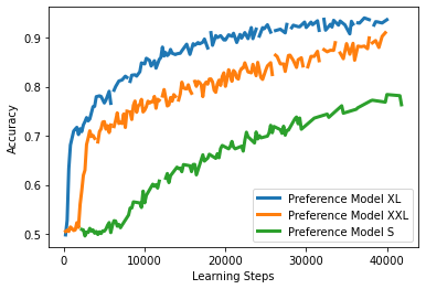
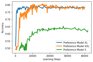
Figure 1: Learning curves showing the accuracy of preference models of different sizes on the train set (left) and on the test set (right).

Our second experiment consists in looking at the accuracy of T5X-XL reward model versus the accuracy of a T5X-XL preference model. We observe that the preference model has a slightly better accuracy than the reward model on the test set (peak accuracy for the preference model is around $0.78$ vs $0.76$ for the reward model).

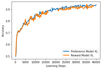
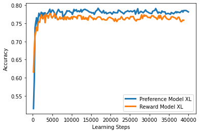
Figure 2: Learning curves showing the accuracy of a preference model versus the accuracy of a reward model of the same size on the train set (left) and on the test set (right).

8.2 Supervised fine-tuned (SFT) initial policy

In all our experiments, we will initialize our policy with a T5X-L model and fine-tune it by supervised learning using the OpenAI dataset described in Stiennon et al. (2020) that was built from the TL;DR dataset (Völske et al., 2017). We call this supervised fine-tuned model the SFT. In all our experiments, our policies are initialized with this SFT.

For all our policy models, we opted for a T5X-L model, as opposed to T5X-XL, for computational efficiency and to compute the pairwise comparisons across our policies. The primary objective of these experiments is to provide a proof of concept for the NLHF approach introduced in this paper, rather than striving for state-of-the-art performance in text summarization. Therefore, our aim is to conduct a fair and equitable comparison among the various approaches.

8.3 RLHF baseline

We established a RLHF baseline by initializing our model with the SFT and then updating the policy by doing 10000 steps of a regularized policy gradient update:

$$\mathbb{E}_{x\sim\rho,y\sim\pi_{\theta}(\cdot|x)}\left[\nabla_{\theta}\log\pi_{\theta}(y|x)\left(R(x,y)-\tau\mbox{KL}(\pi_{\theta}(\cdot|x),\mu(\cdot|x))\right)\right],$$ (12)

where the reward $R(x,y)$ comes from the trained T5X-XL reward model, as described in Subsection 8.1. We conducted a sweep across a set of values ${0.01,0.02,0.05,0.1,0.2}$ for the parameter $\tau$ of the KL-regularization. The value $\tau=0.05$ has been selected for the pairwise comparison table below.

8.4 NLHF algorithms Nash-MD and Nash-EMA

We initialize our policy with the SFT and update the model by executing the Nash-MD-PG and Nash-EMA-PG algorithms as outlined in Section 7. The preference model ${\cal{P}}$ used in these algorithms is derived from the trained T5X-XL model, as described in Subsection 8.1.

We conducted a sweep over the values $\tau\in\{0.02,0.01,0.008,0.005\}$ and selected $\tau=0.008$ for all Nash-MD and Nash-EMA experiments for the pairwise comparison table below.

For Nash-MD-PG we conducted a sweep over the mixing coefficient $\beta\in\{0,0.125,0.250,0.375,0.5,$ $0.625,0.75,0.875,1.0\}$ (used in the definition of the alternative policy defined in Section 7.3) and for Nash-EMA-PG we have swept over $\beta\in\{0,0.999,0.9995,0.9999,1.0\}$.

8.5 Pairwise preference between all the models

Here are the list of all the models we considered for pairwise preference comparison.

• SFT: Supervised-fined-tuned, described in Subsection 8.2. All models all initialised with this SFT and this SFT is also the policy $\mu$ we use for the KL-regularization.

• RLHF described in Subsection 8.3 with regularization coefficient $\tau=0.05$.

• SP (self-play). This corresponds to Nash-MD-PG with mixture coefficient $\beta=0$ (or equivalently Nash-EMA-PG with $\beta=0$ as both algorithms are equivalent for $\beta=0$), described in Subsection 8.4. The policy improves by playing against itself (the alternative policy $\pi^{\prime}=\pi_{\theta}$ is the current policy).

• MD1 to MD6 is Nash-MD-PG with $\beta\in\{0.125,0.25,0.375,0.5,0.625,0.75\}$.

• BR is best-response against SFT. This corresponds to Nash-MD-PG with $\beta=1$ (or equivalently Nash-EMA-PG with $\beta=1$). The policy improves by playing against the fixed SFT policy.

• EMA1 and EMA2 are the last-iterate of Nash-EMA-PG (i.e., returns the last policy), with $\beta\in\{0.999,0.9995\}$.

• EMA1* and EMA* are the EMA policy of Nash-EMA-PG (i.e., returns the policy with average weight) with $\beta\in\{0.999,0.9995\}$.

All models are trained for $10000$ steps. The Nash-MD models (as well as SP and BR) and Nash-EMA are trained with a regularization coefficient of $\tau=0.008$. The pairwise preference comparisons under ${\cal{P}}_{\tau}$ are given in Table 1; these figures are estimated based on 1,000 pairwise comparisons, and hence an upper bound on the width of a 95% confidence interval for each is $\pm 0.032$, based on the exact Clopper-Pearson method for Bernoulli proportions (Clopper and Pearson, 1934). Note that the Clopper-Pearson method can be used to deduce a per-element confidence interval which may be considerably narrower in cases where the empirically observed preference rate is close to 0 or 1.

Table 1: The regularized preference ${\cal{P}}_{\tau}(\pi_{c}\succ\pi_{r})$ between column policy $\pi_{c}$ against row policy $\pi_{r}$

${\cal{P}}_{\tau}$	SFT	RLHF	SP	MD1	MD2	MD3	MD4	MD5	MD6	BR	EMA1	EMA2	EMA1*	EMA2*
SFT	0.500	0.975	0.981	0.986	0.983	0.982	0.979	0.970	0.967	0.933	0.965	0.970	0.971	0.975
RLHF	0.025	0.500	0.741	0.769	0.752	0.744	0.661	0.450	0.340	0.167	0.640	0.531	0.617	0.671
SP	0.019	0.259	0.500	0.547	0.506	0.509	0.406	0.244	0.185	0.082	0.418	0.338	0.363	0.450
MD1	0.014	0.231	0.453	0.500	0.471	0.469	0.354	0.224	0.165	0.079	0.372	0.308	0.348	0.409
MD2	0.017	0.248	0.494	0.529	0.500	0.492	0.393	0.231	0.182	0.084	0.426	0.315	0.375	0.454
MD3	0.018	0.256	0.491	0.531	0.508	0.500	0.380	0.230	0.153	0.087	0.411	0.328	0.349	0.457
MD4	0.021	0.339	0.594	0.646	0.607	0.620	0.500	0.306	0.224	0.088	0.508	0.416	0.458	0.531
MD5	0.030	0.550	0.756	0.776	0.769	0.770	0.694	0.500	0.380	0.169	0.682	0.554	0.627	0.697
MD6	0.033	0.660	0.815	0.835	0.818	0.847	0.776	0.620	0.500	0.269	0.735	0.644	0.706	0.777
BR	0.067	0.833	0.918	0.921	0.916	0.913	0.912	0.831	0.731	0.500	0.856	0.789	0.830	0.875
EMA1	0.035	0.360	0.582	0.628	0.574	0.589	0.492	0.318	0.265	0.144	0.500	0.407	0.448	0.507
EMA2	0.030	0.469	0.662	0.692	0.685	0.672	0.584	0.446	0.356	0.211	0.593	0.500	0.540	0.627
EMA1*	0.029	0.383	0.637	0.652	0.625	0.651	0.542	0.373	0.294	0.170	0.552	0.460	0.500	0.589
EMA2*	0.025	0.329	0.550	0.591	0.546	0.543	0.469	0.303	0.223	0.125	0.493	0.373	0.411	0.500

We will analyse these results after the next section where we describe an evaluation of our models based on a preference model build from a much larger LLM.

8.6 Evaluation using the PaLM 2 preference model

While the ideal approach for evaluating our models would involve soliciting human preferences between summaries generated by different models, we resort to a proxy method using the highly capable LLM, PaLM 2 Large (Anil et al., 2023). We query this model to obtain a preference signal, which we refer to as the PaLM 2 preference model ${\cal{P}}^{*}(y\succ y^{\prime}|x)$, achieved by prompting the LLM in the following manner:

‘You are an expert summary rater. Given a piece of text and two of its

possible summaries, output 1 or 2 to indicate which summary is better.

Text - $$\langle\mbox{text}\rangle \langle\mbox{summary1}\rangle \langle\mbox{summary2}\rangle$$, Summary 1 - , Summary 2 - .

Preferred Summary -’,

where $\langle\mbox{text}\rangle$ corresponds to $x$, $\langle\mbox{summary1}\rangle$ to $y$, and $\langle\mbox{summary2}\rangle$ to $y^{\prime}$.

This evaluation approach shares similarities with the method employed by Lee et al. (2023). To obtain an assessment of the preference ${\cal{P}}^{*}(\pi\succ\pi^{\prime})$, we compute the ratio between the total number of token ’1’ generated and the total number of token ’1’ or ’2’ across $2000$ samples drawn from the distribution $(x\sim\rho,y\sim\pi(\cdot|x),y^{\prime}\sim\pi^{\prime}(\cdot|x))$.

This ${\cal{P}}^{*}$ serves as an approximate surrogate for human preferences. Notably, it is essential to highlight that the preference model ${\cal{P}}$ utilized during the training of our policies is considerably smaller in size than ${\cal{P}}^{*}$ and corresponds to a different model. Specifically, ${\cal{P}}$ is based on the T5X-XL model, fine-tuned with TL;DR data, whereas ${\cal{P}}^{*}$ is derived from the PaLM 2 Large model.

The pairwise preference comparisons under ${\cal{P}}^{*}$ using the PaLM 2 Large model are given in Table 2. As each element is estimated with $2000$ samples, the confidence interval, an upper bound on the 95% confidence interval is given by $\pm 0.023$, based on the exact Clopper-Pearson method for Bernoulli proportions (Clopper and Pearson, 1934).

Table 2: PaLM 2 preference ${\cal{P}}^{*}(\pi_{c}\succ\pi_{r})$ model between column policy $\pi_{c}$ against row policy $\pi_{r}$.

${\cal{P}}^{*}$	SFT	RLHF	SP	MD1	MD2	MD3	MD4	MD5	MD6	BR	EMA1	EMA2	EMA1*	EMA2*
SFT	0.500	0.990	0.983	0.982	0.989	0.987	0.985	0.982	0.965	0.943	0.970	0.961	0.977	0.980
RLHF	0.010	0.500	0.489	0.598	0.519	0.561	0.501	0.436	0.284	0.148	0.468	0.320	0.477	0.510
SP	0.017	0.511	0.500	0.592	0.504	0.545	0.499	0.451	0.310	0.211	0.445	0.362	0.464	0.488
MD1	0.018	0.402	0.408	0.500	0.425	0.470	0.369	0.362	0.238	0.163	0.391	0.270	0.400	0.447
MD2	0.011	0.481	0.496	0.575	0.500	0.513	0.491	0.434	0.298	0.196	0.460	0.351	0.430	0.496
MD3	0.013	0.439	0.455	0.530	0.487	0.500	0.484	0.408	0.273	0.187	0.429	0.323	0.413	0.472
MD4	0.015	0.499	0.501	0.631	0.509	0.516	0.500	0.428	0.265	0.161	0.468	0.358	0.437	0.503
MD5	0.018	0.564	0.549	0.638	0.566	0.592	0.572	0.500	0.329	0.210	0.532	0.389	0.518	0.539
MD6	0.035	0.716	0.690	0.762	0.702	0.727	0.735	0.671	0.500	0.342	0.652	0.548	0.651	0.691
BR	0.057	0.852	0.789	0.837	0.804	0.813	0.839	0.790	0.658	0.500	0.743	0.640	0.752	0.774
EMA1	0.030	0.532	0.555	0.609	0.540	0.571	0.532	0.468	0.348	0.257	0.500	0.381	0.480	0.556
EMA2	0.039	0.680	0.638	0.730	0.649	0.677	0.642	0.611	0.452	0.360	0.619	0.500	0.585	0.659
EMA1*	0.023	0.523	0.536	0.600	0.570	0.587	0.563	0.482	0.349	0.248	0.520	0.415	0.500	0.555
EMA2*	0.020	0.490	0.512	0.553	0.504	0.528	0.497	0.461	0.309	0.226	0.444	0.341	0.445	0.500

8.7 Analysis of the results

First, let us mention that the RLHF baseline that we have built is a very strong baseline. It beats SFT with a win rate of $99\%$ marking the highest win rate observed against SFT among all models when using the PaLM 2 preference model ${\cal{P}}^{*}$

Best-response against self-play (BR) does not exhibit strong performance. Despite being trained explicitly to outperform self-play during training, its ${\cal{P}}^{*}$-evaluation yields a relatively modest score of $94\%$ against self-play. Furthermore, BR performs poorly against RLHF and all other Nash-based approaches. This suggests the possibility of ’preference hacking,’ where BR may be overly adapting to the preference model by overfitting to the specific SFT policy.

Self-play (SP) exhibits strong overall performance, with notable exceptions in the ${\cal{P}}^{*}$ evaluation against RLHF and the Nash-MD models (for $\beta\leq 0.5$). This suggests that enhancing one’s policy through self-play could be a promising avenue for improving the initial model. However, it’s essential to acknowledge that self-play does not guarantee the attainment of a Nash equilibrium, as cyclic patterns are possible, as discussed in the Theory Section. In particular, SP is found to be vulnerable to exploitation by certain Nash-MD models.

The Nash-MD models, especially those with $\beta\leq 0.5$, exhibit very strong performance. Notably, Nash-MD models with $\beta=0.125$, $\beta=0.25$, and $\beta=0.375$ outperform all other models, including RLHF. Among them, Nash-MD with $\beta=0.125$ (highlighted in bold as ’MD1’) emerges as the top-performing model, surpassing all others in both the training preference model ${\cal{P}}_{\tau}$ and the evaluation model ${\cal{P}}^{*}$.

All Nash-EMA models, including EMA1 and EMA2 (representing the last iterate) as well as EMA1* and EMA2* (representing the average policy), are outperformed by Nash-MD for $\beta\leq 0.5$ and RLHF. This observation may suggest that the first-order approximation of the mixture policy as the policy having an average (EMA) weight may not be well-suited in this context, potentially contributing to the overall lower performance.

Examining Nash-MD, which emerges as the most efficient method, it is interesting to note that both extreme values of the mixing parameter $\beta\in[0,1]$, namely $\beta=0$ (self-play) and $\beta=1$ (best-response against SFT), result in suboptimal performance compared to intermediate values of $\beta$ (particularly $\beta=0.125$, $\beta=0.25$, and $\beta=0.375$). This trend is visible, for instance, in the highlighted blue row showing Nash-MD (for $\beta\in{0,0.125,0.25,0.375,0.5,0.625,0.75,1.0}$) against RLHF. It suggests that improving one’s policy by playing against a mixture of the initial policy and the current policy yields superior model improvement compared to interactions with either the initial policy or the current policy in isolation.

9 Conclusion and future work

NLHF emerges as an interesting and promising alternative to RLHF, offering a fresh perspective on aligning models with human preferences. Learning a preference model from human preference data is a more intuitive and natural approach compared to learning a reward model. It involves simpler techniques, such as supervised learning, and doesn’t necessitate specific assumptions, like the Bradley-Terry model.

Once a preference model is established, the concept of the Nash equilibrium naturally arises as a compelling solution concept. Nash-MD, an algorithm that optimizes policies by playing against a geometric mixture of the current policy and the initial policy, has been introduced. We have established its last-iterate convergence to the Nash equilibrium.

We have introduced and implemented deep learning versions of Nash-MD and Nash-EMA in LLMs and reported results in a text-summarization task. For Nash-EMA-PG, we considered both the last-iterate and the average policy. Both Nash-MD-PG and Nash-EMA-PG demonstrate competitive performance compared to the RLHF baseline.

Nash-MD-PG stands out as the best-performing method, surpassing other models in a pairwise comparison, when evaluated with a very large LLM (PaLM 2 Large). The choice of the mixture parameter in Nash-MD entails an interesting trade-off. A parameter value of 0 corresponds to self-play, while a value of 1 represents best-response against SFT. Notably, intermediate values within the range of 0.125 to 0.375 consistently outperform both self-play and best-response, highlighting the advantages of playing against a mixture of policies as opposed to a pure policy.

Future research directions would consider the exploration of various mixtures between the current policy and past checkpoints, extending the concept initially introduced by Nash-MD. Additionally, another immediate direction would consider incorporating a decaying mixing coefficient $\beta$ to align more closely with theoretical considerations.

In conclusion, NLHF offers a compelling avenue for preference learning and policy optimization. The introduction of Nash-MD as an algorithmic solution, along with deep learning adaptations, opens up new possibilities for aligning models with human preferences. Further research in this direction, including the exploration of different mixture strategies, holds significant promise for advancing the field of aligning LLMs with human preferences.

Appendix A Maximizing expected Elo vs maximizing probability of winning

Consider the following preference model, where the set of actions is $\mathcal{Y}=\{y_{1},y_{2},y_{3}\}$ and the preference table between these actions is

${\cal{P}}(y\succ y^{\prime})$	$y=y_{1}$	$y=y_{2}$	$y=y_{3}$
$y^{\prime}=y_{1}$	1/2	9/10	2/3
$y^{\prime}=y_{2}$	1/10	1/2	2/11
$y^{\prime}=y_{3}$	1/3	9/11	1/2

This preference model can be perfectly captured by a Bradley-Terry reward model in which the Elo score of all actions would be (up to an additive constant): $R(y_{1})=0$, $R(y_{2})=\log 9$, and $R(y_{3})=\log 2$.

If we optimize over the simplex $\Delta(\mathcal{Y})$, then the policy selecting deterministically $y_{2}$ is optimal both in terms of rewards and in terms of preference against any policy. However, if we consider a constrained optimization problem where we search for a policy in a subset ${\cal S}\subset\Delta(\mathcal{Y})$, then the optimum of the expected reward and preference may be different. To illustrate, let ${\cal S}$ be the set of probability distributions $\pi\in\Delta(\mathcal{Y})$ such that $\pi(y_{1})=2\pi(y_{2})$.

In that case, the policy $\pi^{*}_{R}\stackrel{{\scriptstyle\rm def}}{{=}}(2/3,1/3,0)$ is optimal in terms of maximizing expected rewards whereas the policy $\pi^{*}_{{\cal{P}}}\stackrel{{\scriptstyle\rm def}}{{=}}(0,0,1)$ is optimal in terms of maximizing preference against any alternative policy in ${\cal S}$. In particular we have

$$\mathbb{E}_{y\sim\pi^{*}_{R}}[R(y)]=0\times 2/3+\log(9)\times 1/3>\log(2)=\mathbb{E}_{y\sim\pi^{*}_{{\cal{P}}}}[R(y)],$$

whereas policy $\pi^{*}_{{\cal{P}}}$ is preferred over $\pi^{*}_{R}$, since

$${\cal{P}}(\pi^{*}_{{\cal{P}}}\succ\pi^{*}_{R})={\cal{P}}(y_{3}\succ y_{1})\times 2/3+{\cal{P}}(y_{3}\succ y_{2})\times 1/3=50/99>1/2.$$

Thus if one searches for a policy in ${\cal S}$, then the optimum in terms of maximizing expected (Elo) reward and maximizing preference (probability of winning) are different.

Note that the constraint $\pi\in{\cal S}$ may be imposed in a soft way using regularization. Here for example we could implement a 2-step decisions process where in a first step one would choose the probability mass assigned to $y_{3}$, and in the second step, one would choose the remaining mass to allocate between $y_{1}$ and $y_{2}$. The second step may be constrained in a soft way by penalizing distributions (over $y_{1}$ and $y_{2}$) that are different from a reference distribution $\mu=(2/3,1/3)$ by using a KL-regularization with a large $\tau$ coefficient. In this way the set of effective policies that would be considered would be close to ${\cal S}$.

This example illustrates the fact that in constrained (or regularized) optimization settings, maximizing Elo versus preference are different objectives, even in a setting where preferences can be perfectly expressed in a Bradley-Terry model.

Appendix B Proof of Theorem 1

We start with a first lemma.

Lemma 1.

For any $\pi$, and $0\leq\eta\tau\leq 1$, we have

$$\mbox{KL}(\pi,\pi_{t}^{\mu})\leq\eta\tau\mbox{KL}(\pi,\mu)+(1-\eta\tau)\mbox{KL}(\pi,\pi_{t})-\eta\tau\mbox{KL}(\pi_{t}^{\mu},\mu).$$

Proof.

From the definition of $\pi_{t}^{\mu}$, we have

$$\log\pi_{t}^{\mu}(y)=(1-\eta\tau)\log\pi_{t}(y)+\eta\tau\log\mu(y)-\log Z,$$

where we define $Z=\sum_{y^{\prime}}(\pi_{t}(y^{\prime}))^{1-\eta\tau}(\mu(y^{\prime}))^{\eta\tau}$. Thus, for any $\pi$, we have

$$\mbox{KL}(\pi,\pi_{t}^{\mu})=\eta\tau\mbox{KL}(\pi,\mu)+(1-\eta\tau)\mbox{KL}(\pi,\pi_{t})+\log Z.$$

We have that

$$\eta\tau\mbox{KL}(\pi_{t}^{\mu},\mu) = \eta\tau\sum_{y}\pi_{t}^{\mu}(y)\log\frac{\big{(}\pi_{t}(y)\big{)}^{1-\eta\tau}\big{(}\mu(y)\big{)}^{\eta\tau}}{Z\mu(y)}$$

$$= (1-\eta\tau)\sum_{y}\pi_{t}^{\mu}(y)\log\frac{\big{(}\pi_{t}(y)\big{)}^{\eta\tau}}{\big{(}\mu(y)\big{)}^{\eta\tau}}-\eta\tau\log Z$$

$$\leq (1-\eta\tau)\log\sum_{y}\pi_{t}^{\mu}(y)\frac{\big{(}\pi_{t}(y)\big{)}^{\eta\tau}}{\big{(}\mu(y)\big{)}^{\eta\tau}}-\eta\tau\log Z$$

$$= (1-\eta\tau)\log\sum_{y}\frac{\big{(}\pi_{t}(y)\big{)}^{1-\eta\tau}\big{(}\mu(y)\big{)}^{\eta\tau}}{Z}\frac{\big{(}\pi_{t}(y)\big{)}^{\eta\tau}}{\big{(}\mu(y)\big{)}^{\eta\tau}}-\eta\tau\log Z$$

$$= -\log Z,$$

where we used Jensen’s inequality applied with the concave logarithmic function. We deduce

$$\mbox{KL}(\pi,\pi_{t}^{\mu})\leq\eta\tau\mbox{KL}(\pi,\mu)+(1-\eta\tau)\mbox{KL}(\pi,\pi_{t})-\eta\tau\mbox{KL}(\pi_{t}^{\mu},\mu).$$

∎

Now we use Lemma 7 of Munos et al. (2020), restated below with notation.

Lemma 2.

Let $p\geq 1$ and $q\geq 1$ such that $1/p+1/q=1$. Let $\varphi$ be a strongly convex function with respect to the $\ell_{p}$-norm $\|\cdot\|_{p}$ with some modulus $\sigma$, i.e., for any $\pi,\pi^{\prime}$,

$$\varphi(\pi)\geq\varphi(\pi^{\prime})+\nabla\varphi(\pi^{\prime})\cdot(\pi-\pi^{\prime})+\frac{\sigma}{2}\|\pi-\pi^{\prime}\|^{2}.$$

Write $D_{\varphi}$ the associated Bregman divergence: for $\pi,\pi^{\prime}$,

$$D_{\varphi}(\pi,\pi^{\prime})\stackrel{{\scriptstyle\rm def}}{{=}}\varphi(\pi)-\varphi(\pi^{\prime})-\nabla\varphi(\pi^{\prime})\cdot(\pi-\pi^{\prime}).$$

Let $\delta$ be a vector of dimension $|\mathcal{Y}|$. For any $\pi^{-}\in\Delta(\mathcal{Y})$, define $\pi^{+}$ as

$$\pi^{+}=\arg\max_{\pi\in\Delta(\mathcal{Y})}\left[\sum_{y}\pi(y)\delta(y)-D_{\varphi}(\pi,\pi^{-})\right],$$ (13)

Then for any $\pi\in\Delta(\mathcal{Y})$, we have,

$$D_{\varphi}(\pi,\pi^{+})\leq D_{\varphi}(\pi,\pi^{-})+\sum_{y}(\pi^{-}(y)-\pi(y))\delta(y)+(2/\sigma)\|\delta\|_{q}^{2}.$$

We apply this lemma with $\pi^{+}=\pi_{t+1}$ and $\pi^{-}=\pi_{t}^{\mu}$, with the vector $\delta(y)=\eta{\cal{P}}(y\succ\pi_{t}^{\mu})$, and as Bregman divergence $D_{\varphi}$ we choose the KL (which corresponds to the choice of the entropy regularizer $\varphi(\pi)=\sum_{y}\pi(y)\log\pi(y)$). For $p=1$, $q=\infty$, the regularizer $\varphi$ is a strongly convex function with respect to the $\ell_{1}$-norm with a modulus $\sigma=1$; this is a consequence of Pinsker’s inequality, see Csiszar and Korner (1982).

We deduce that for any $\pi$,

$$\mbox{KL}(\pi,\pi_{t+1})\leq\mbox{KL}(\pi,\pi_{t}^{\mu})+\eta\sum_{y}(\pi_{t}^{\mu}(y)-\pi(y)){\cal{P}}(y\succ\pi_{t}^{\mu})+2\eta^{2}.$$ (14)

For the choice $\pi=\pi^{*}_{\tau}$ and using the previous lemma, we have

$$\mbox{KL}(\pi^{*}_{\tau},\pi_{t+1}) \leq \mbox{KL}(\pi^{*}_{\tau},\pi_{t}^{\mu})+\eta\sum_{y}(\pi_{t}^{\mu}(y)-\pi^{*}_{\tau}(y)){\cal{P}}(y\succ\pi_{t}^{\mu})+2\eta^{2}$$

$$\leq (1-\eta\tau)\mbox{KL}(\pi^{*}_{\tau},\pi_{t})+\eta\tau\left(\mbox{KL}(\pi^{*}_{\tau},\mu)-\mbox{KL}(\pi_{t}^{\mu},\mu)\right)$$

$$+\eta\left({\cal{P}}(\pi_{t}^{\mu}\succ\pi_{t}^{\mu})-{\cal{P}}(\pi^{*}_{\tau}\succ\pi_{t}^{\mu})\right)+2\eta^{2}$$

$$= (1-\eta\tau)\mbox{KL}(\pi^{*}_{\tau},\pi_{t})+\eta\left[1/2-{\cal{P}}(\pi^{*}_{\tau}\succ\pi_{t}^{\mu})+\tau\mbox{KL}(\pi^{*}_{\tau},\mu)-\tau\mbox{KL}(\pi_{t}^{\mu},\mu)\right]+2\eta^{2}$$

$$= (1-\eta\tau)\mbox{KL}(\pi^{*}_{\tau},\pi_{t})+\eta\left[1/2-{\cal{P}}_{\tau}(\pi^{*}_{\tau}\succ\pi_{t}^{\mu})\right]+2\eta^{2}$$

$$\leq (1-\eta\tau)\mbox{KL}(\pi^{*}_{\tau},\pi_{t})+2\eta^{2},$$

where the last inequality comes from the fact that $\pi_{\tau}^{*}$ is the Nash of the regularized game ${\cal{P}}_{\tau}$: ${\cal{P}}_{\tau}(\pi^{*}_{\tau}\succ\pi_{t}^{\mu})\geq{\cal{P}}_{\tau}(\pi^{*}_{\tau}\succ\pi^{*}_{\tau})=1/2$ and the last equality comes from the definition of the regularized preference.

By iterating this inequality we deduce

$$\mbox{KL}(\pi^{*}_{\tau},\pi_{T}) \leq 2\eta^{2}\sum_{t=0}^{T-1}(1-\eta\tau)^{i}+(1-\eta\tau)^{T}\mbox{KL}(\pi^{*}_{\tau},\pi_{0})$$

$$\leq 2\frac{\eta}{\tau}+e^{-\eta\tau T}\mbox{KL}(\pi^{*}_{\tau},\pi_{0}).$$

We deduce that for the choice $\eta=\log T/(\tau T)$ we have

$$\mbox{KL}(\pi^{*}_{\tau},\pi_{T})\leq\left(\mbox{KL}(\pi^{*}_{\tau},\pi_{0})+\frac{2\log T}{\tau^{2}}\right)\frac{1}{T}\cdot$$

Appendix C Proof of Proposition 1

To prove existence and uniqueness of Nash equilibrium we first note that since ${\cal{P}}_{\tau}(\pi^{\prime}\succ\pi)=1-{\cal{P}}_{\tau}(\pi\succ\pi^{\prime})$ we can re-express the minimax game of Eq. 2 as a symmetric two-player game with payoffs of policy $\pi$ and $\pi^{\prime}$ are defined as

$$R(\pi;\pi^{\prime})={\cal{P}}(\pi\succ\pi^{\prime})-\tau\mbox{KL}_{\rho}(\pi,\mu)$$

and

$$R(\pi^{\prime};\pi)={\cal{P}}(\pi^{\prime}\succ\pi)-\tau\mbox{KL}_{\rho}(\pi^{\prime},\mu)$$

respectively. First we notice that since the payoff of this game is concave in $\pi$ and $\pi^{\prime}$, it possesses a Nash equilibrium (Rosen, 1965, Theorem 1).

To show that this game has unique Nash equilibrium we need to show that its corresponding variational inequality is strictly monotone (Rosen, 1965, Theorem 2). Let $\bar{\pi}=[\pi,\pi^{\prime}]$ and $v(\bar{\pi})=[\nabla_{\pi}R(\pi;\pi^{\prime}),\nabla_{\pi^{\prime}}R(\pi^{\prime};\pi)]$. Then every Nash equilibrium of the game should satisfy the following variational inequality for all $\bar{\pi}$:

$$v^{T}(\bar{\pi}^{*})(\bar{\pi}^{*}-\bar{\pi})\leq 0$$

Furthermore the variational inequality is strictly monotone if and only if for every $\bar{\pi}_{1}$ and $\bar{\pi}_{2}$ we have that

$$(v(\bar{\pi}_{1})-v(\bar{\pi}_{2}))^{T}(\bar{\pi}_{1}-\bar{\pi}_{2})\leq 0$$ (15)

with equality only holds at $\bar{\pi}_{1}=\bar{\pi}_{2}$ (Rosen, 1965, Theorem 2). We can show this inequality holds by expanding the terms on LHS. For every context $x$ let denote $v(\bar{\pi})(x)$ as the partial derivative $v(\bar{\pi})$ for $x$. We have:

$$v(\bar{\pi})(x)=\rho(x)[\mathbf{P}(y\succ\pi^{\prime}|x)-\tau\log(\pi/\mu|x)-1,\mathbf{P}(y\succ\pi|x)-\tau\log(\pi^{\prime}/\mu|x)-1],$$

where $\mathbf{P}(y\succ\pi^{\prime}|x)=[p(y_{i}\succ\pi|x)]_{i=1:N}$ and $\log(\pi/\mu|x)=[\log(\pi(y_{i}|x)/\mu(y_{i}|x))]_{i=1:N}$, in which $N$ is the size of the generation set. Plugging this in the LHS of Eq.15 and then exploiting the non-negativity of KL-divergence implies:

$$(v(\bar{\pi}_{1})-v(\bar{\pi}_{2}))^{T}(\bar{\pi}_{1}-\bar{\pi}_{2}) =\underbrace{{\cal{P}}(\pi_{1}\succ\pi^{\prime}_{1})+{\cal{P}}(\pi^{\prime}_{1}\succ\pi_{1})+{\cal{P}}(\pi_{2}\succ\pi^{\prime}_{2})+{\cal{P}}(\pi^{\prime}_{2}\succ\pi_{2})}_{=2}$$

$$-\underbrace{({\cal{P}}(\pi_{2}\succ\pi^{\prime}_{1})+{\cal{P}}(\pi^{\prime}_{1}\succ\pi_{2})+{\cal{P}}(\pi_{1}\succ\pi^{\prime}_{2})+{\cal{P}}(\pi^{\prime}_{2}\succ\pi_{1}))}_{=2}$$

$$-\tau(\mbox{KL}_{\rho}(\pi_{1}||\pi_{2})+\mbox{KL}_{\rho}(\pi_{2}||\pi_{1})+\mbox{KL}_{\rho}(\pi^{\prime}_{1}||\pi^{\prime}_{2})+\mbox{KL}_{\rho}(\pi^{\prime}_{2}||\pi^{\prime}_{1}))$$

$$=-\tau(\mbox{KL}_{\rho}(\pi_{1}||\pi_{2})+\mbox{KL}_{\rho}(\pi_{2}||\pi_{1})+\mbox{KL}_{\rho}(\pi^{\prime}_{1}||\pi^{\prime}_{2})+\mbox{KL}_{\rho}(\pi^{\prime}_{2}||\pi^{\prime}_{1}))\leq 0$$

with equality only at $\bar{\pi}_{1}=\bar{\pi}_{2}$.

References

- Abernethy et al. (2018) J. Abernethy, K. A. Lai, K. Y. Levy, and J.-K. Wang. Faster rates for convex-concave games. Proceedings of the Annual Conference on Learning Theory, 2018.
- Akrour et al. (2011) R. Akrour, M. Schoenauer, and M. Sebag. Preference-based policy learning. In D. Gunopulos, T. Hofmann, D. Malerba, and M. Vazirgiannis, editors, Machine Learning and Knowledge Discovery in Databases, 2011.
- Amodei et al. (2016) D. Amodei, C. Olah, J. Steinhardt, P. Christiano, J. Schulman, and D. Mané. Concrete problems in AI safety. arXiv, 2016.
- Anil et al. (2023) R. Anil, A. M. Dai, O. Firat, M. Johnson, D. Lepikhin, A. Passos, S. Shakeri, E. Taropa, P. Bailey, Z. Chen, E. Chu, J. H. Clark, L. E. Shafey, Y. Huang, K. Meier-Hellstern, G. Mishra, E. Moreira, M. Omernick, K. Robinson, S. Ruder, Y. Tay, K. Xiao, Y. Xu, Y. Zhang, G. H. Abrego, J. Ahn, J. Austin, P. Barham, J. Botha, J. Bradbury, S. Brahma, K. Brooks, M. Catasta, Y. Cheng, C. Cherry, C. A. Choquette-Choo, A. Chowdhery, C. Crepy, S. Dave, M. Dehghani, S. Dev, J. Devlin, M. Díaz, N. Du, E. Dyer, V. Feinberg, F. Feng, V. Fienber, M. Freitag, X. Garcia, S. Gehrmann, L. Gonzalez, G. Gur-Ari, S. Hand, H. Hashemi, L. Hou, J. Howland, A. Hu, J. Hui, J. Hurwitz, M. Isard, A. Ittycheriah, M. Jagielski, W. Jia, K. Kenealy, M. Krikun, S. Kudugunta, C. Lan, K. Lee, B. Lee, E. Li, M. Li, W. Li, Y. Li, J. Li, H. Lim, H. Lin, Z. Liu, F. Liu, M. Maggioni, A. Mahendru, J. Maynez, V. Misra, M. Moussalem, Z. Nado, J. Nham, E. Ni, A. Nystrom, A. Parrish, M. Pellat, M. Polacek, A. Polozov, R. Pope, S. Qiao, E. Reif, B. Richter, P. Riley, A. C. Ros, A. Roy, B. Saeta, R. Samuel, R. Shelby, A. Slone, D. Smilkov, D. R. So, D. Sohn, S. Tokumine, D. Valter, V. Vasudevan, K. Vodrahalli, X. Wang, P. Wang, Z. Wang, T. Wang, J. Wieting, Y. Wu, K. Xu, Y. Xu, L. Xue, P. Yin, J. Yu, Q. Zhang, S. Zheng, C. Zheng, W. Zhou, D. Zhou, S. Petrov, and Y. Wu. PaLM 2 technical report, 2023.
- Azar et al. (2023) M. G. Azar, M. Rowland, B. Piot, D. Guo, D. Calandriello, M. Valko, and R. Munos. A general theoretical paradigm to understand learning from human preferences. arXiv, 2023.
- Bai et al. (2022) Y. Bai, A. Jones, K. Ndousse, A. Askell, A. Chen, N. DasSarma, D. Drain, S. Fort, D. Ganguli, T. Henighan, N. Joseph, S. Kadavath, J. Kernion, T. Conerly, S. El-Showk, N. Elhage, Z. Hatfield-Dodds, D. Hernandez, T. Hume, S. Johnston, S. Kravec, L. Lovitt, N. Nanda, C. Olsson, D. Amodei, T. Brown, J. Clark, S. McCandlish, C. Olah, B. Mann, and J. Kaplan. Training a helpful and harmless assistant with reinforcement learning from human feedback. arXiv, 2022.
- Bertrand et al. (2023) Q. Bertrand, W. M. Czarnecki, and G. Gidel. On the limitations of the Elo: Real-world games are transitive, not additive. In Proceedings of the International Conference on Artificial Intelligence and Statistics, 2023.
- Bradley and Terry (1952) R. A. Bradley and M. E. Terry. Rank analysis of incomplete block designs: I. the method of paired comparisons. Biometrika, 39(3/4):324–345, 1952.
- Brown (1951) G. W. Brown. Iterative solution of games by fictitious play. Act. Anal. Prod Allocation, 13(1):374, 1951.
- Bubeck (2015) S. Bubeck. Convex optimization: Algorithms and complexity. Foundations and Trends in Machine Learning, 8(3-4):231–357, 2015.
- Busa-Fekete et al. (2013) R. Busa-Fekete, B. Szörenyi, P. Weng, W. Cheng, and E. Hüllermeier. Preference-based evolutionary direct policy search. In Autonomous Learning Workshop at the IEEE International Conference on Robotics and Automation, 2013.
- Busa-Fekete et al. (2014) R. Busa-Fekete, B. Szörényi, P. Weng, W. Cheng, and E. Hüllermeier. Preference-based reinforcement learning: Evolutionary direct policy search using a preference-based racing algorithm. Machine Learning, 97(3):327–351, 2014.
- Busbridge et al. (2023) D. Busbridge, J. Ramapuram, P. Ablin, T. Likhomanenko, E. G. Dhekane, X. Suau, and R. Webb. How to scale your EMA. arXiv, 2023.
- Cesa-Biachi and Lugosi (2006) N. Cesa-Biachi and G. Lugosi. Predition, Learning, and Games. Cambridge University Press, 2006.
- Chen et al. (2022) X. Chen, H. Zhong, Z. Yang, Z. Wang, and L. Wang. Human-in-the-loop: Provably efficient preference-based reinforcement learning with general function approximation. arXiv, 2022.
- Cheng et al. (2011) W. Cheng, J. Fürnkranz, E. Hüllermeier, and S.-H. Park. Preference-based policy iteration: Leveraging preference learning for reinforcement learning. In D. Gunopulos, T. Hofmann, D. Malerba, and M. Vazirgiannis, editors, Machine Learning and Knowledge Discovery in Databases, 2011.
- Christiano et al. (2017) P. Christiano, J. Leike, T. B. Brown, M. Martic, S. Legg, and D. Amodei. Deep reinforcement learning from human preferences. In Advances in Neural Information Processing Systems, 2017.
- Clopper and Pearson (1934) C. J. Clopper and E. S. Pearson. The use of confidence or fiducial limits illustrated in the case of the binomial. Biometrika, 26(4):404–413, 1934.
- Csiszar and Korner (1982) I. Csiszar and J. Korner. Information Theory: Coding Theorems for Discrete Memoryless Systems. Academic Press, Inc., USA, 1982.
- Daskalakis and Panageas (2019) C. Daskalakis and I. Panageas. Last-iterate convergence: Zero-sum games and constrained min-max optimization. In Proceedings of the Conference on Innovations in Theoretical Computer Science, 2019.
- Daskalakis et al. (2011) C. Daskalakis, A. Deckelbaum, and A. Kim. Near-optimal no-regret algorithms for zero-sum games. In ACM-SIAM Symposium on Discrete Algorithms, 2011.
- Efroni et al. (2021) Y. Efroni, N. Merlis, and S. Mannor. Reinforcement learning with trajectory feedback. In Proceedings of the AAAI Conference on Artificial Intelligence, 2021.
- Elo (1978) A. E. Elo. The Rating of Chessplayers, Past and Present. Arco Pub., 1978.
- Farina et al. (2019) G. Farina, C. Kroer, and T. Sandholm. Optimistic regret minimization for extensive-form games via dilated distance-generating functions. In Advances in Neural Information Processing Systems, 2019.
- Fudenberg and Levine (1998) D. Fudenberg and D. K. Levine. The theory of learning in games. MIT Press, 1998.
- Gardner (1970) M. Gardner. The paradox of the nontransitive dice. Scientific American, (223):110–111, 1970.
- Geist et al. (2019) M. Geist, B. Scherrer, and O. Pietquin. A theory of regularized Markov decision processes. In Proceedings of the International Conference on Machine Learning, 2019.
- Gidel et al. (2016) G. Gidel, T. Jebara, and S. Lacoste-Julien. Frank-Wolfe algorithms for saddle point problems. In Proceedings of the Artificial Intelligence and Statistics, 2016.
- Glaese et al. (2022) A. Glaese, N. McAleese, M. Trebacz, J. Aslanides, V. Firoiu, T. Ewalds, M. Rauh, L. Weidinger, M. Chadwick, P. Thacker, L. Campbell-Gillingham, J. Uesato, P.-S. Huang, R. Comanescu, F. Yang, A. See, S. Dathathri, R. Greig, C. Chen, D. Fritz, J. S. Elias, R. Green, S. Mokrá, N. Fernando, B. Wu, R. Foley, S. Young, I. Gabriel, W. Isaac, J. Mellor, D. Hassabis, K. Kavukcuoglu, L. A. Hendricks, and G. Irving. Improving alignment of dialogue agents via targeted human judgements. arXiv, 2022.
- Grill et al. (2020) J.-B. Grill, F. Strub, F. Altché, C. Tallec, P. H. Richemond, E. Buchatskaya, C. Doersch, B. A. Pires, Z. D. Guo, M. G. Azar, B. Piot, K. Kavukcuoglu, R. Munos, and M. Valko. Bootstrap your own latent: A new approach to self-supervised learning. In Advances in Neural Information Processing Systems, 2020.
- Heinrich and Silver (2016) J. Heinrich and D. Silver. Deep reinforcement learning from self-play in imperfect-information games. arXiv, 2016.
- Heinrich et al. (2015) J. Heinrich, M. Lanctot, and D. Silver. Fictitious self-play in extensive-form games. In Proceedings of the International Conference on Machine Learning, 2015.
- Hennes et al. (2020) D. Hennes, D. Morrill, S. Omidshafiei, R. Munos, J. Perolat, M. Lanctot, A. Gruslys, J. B. Lespiau, P. Parmas, E. Duéñez-Guzmán, and K. Tuyls. Neural replicator dynamics: Multiagent learning via hedging policy gradients. In Proceedings of the International Joint Conference on Autonomous Agents and Multiagent Systems, 2020.
- Hoda et al. (2010) S. Hoda, A. Gilpin, J. Pena, and T. Sandholm. Smoothing techniques for computing Nash equilibria of sequential games. Mathematics of Operations Research, 35(2):494–512, 2010.
- Hofbauer and Sorin (2006) J. Hofbauer and S. Sorin. Best response dynamics for continuous zero-sum games. Discrete and Continuous Dynamical Systems Series B, 6(1):215, 2006.
- Jaques et al. (2019) N. Jaques, A. Ghandeharioun, J. H. Shen, C. Ferguson, A. Lapedriza, N. Jones, S. Gu, and R. Picard. Way off-policy batch deep reinforcement learning of implicit human preferences in dialog. arXiv, 2019.
- Kangarshahi et al. (2018) E. A. Kangarshahi, Y.-P. Hsieh, M. F. Sahin, and V. Cevher. Let’s be honest: An optimal no-regret framework for zero-sum games. In Proceedings of the International Conference on Machine Learning, 2018.
- Klimenko (2015) A. Y. Klimenko. Intransitivity in theory and in the real world. Entropy, 17(6):4364–4412, 2015.
- Korpelevich (1976) G. Korpelevich. The extragradient method for finding saddle points and other problems. Matecon, 12:747–756, 1976.
- Lattimore and Szepesvári (2020) T. Lattimore and C. Szepesvári. Bandit Algorithms. Cambridge University Press, 2020.
- Lee et al. (2023) H. Lee, S. Phatale, H. Mansoor, K. Lu, T. Mesnard, C. Bishop, V. Carbune, and A. Rastogi. RLAIF: Scaling reinforcement learning from human feedback with AI feedback. arXiv, 2023.
- Menick et al. (2022) J. Menick, M. Trebacz, V. Mikulik, J. Aslanides, F. Song, M. Chadwick, M. Glaese, S. Young, L. Campbell-Gillingham, G. Irving, and N. McAleese. Teaching language models to support answers with verified quotes. arXiv, 2022.
- Mertikopoulos et al. (2018) P. Mertikopoulos, C. Papadimitriou, and G. Piliouras. Cycles in adversarial regularized learning. In ACM-SIAM Symposium on Discrete Algorithms, 2018.
- Mertikopoulos et al. (2019) P. Mertikopoulos, B. Lecouat, H. Zenati, C. Foo, V. Chandrasekhar, and G. Piliouras. Optimistic mirror descent in saddle-point problems: Going the extra (gradient) mile. In Proceedings of the International Conference on Learning Representations, 2019.
- Mokhtari et al. (2020) A. Mokhtari, A. Ozdaglar, and S. Pattathil. A unified analysis of extra-gradient and optimistic gradient methods for saddle point problems: Proximal point approach. In Proceedings of the International Conference on Artificial Intelligence and Statistics, 2020.
- Munos et al. (2020) R. Munos, J. Perolat, J.-B. Lespiau, M. Rowland, B. De Vylder, M. Lanctot, F. Timbers, D. Hennes, S. Omidshafiei, A. Gruslys, M. G. Azar, E. Lockhart, and K. Tuyls. Fast computation of Nash equilibria in imperfect information games. In Proceedings of the International Conference on Machine Learning, 2020.
- Nakano et al. (2021) R. Nakano, J. Hilton, S. Balaji, J. Wu, L. Ouyang, C. Kim, C. Hesse, S. Jain, V. Kosaraju, W. Saunders, X. Jiang, K. Cobbe, T. Eloundou, G. Krueger, K. Button, M. Knight, B. Chess, and J. Schulman. WebGPT: Browser-assisted question-answering with human feedback. arXiv, 2021.
- Nemirovski and Yudin (1983) A. Nemirovski and D. Yudin. Problem complexity and method efficiency in optimization. Wiley-Interscience Series in Discrete Mathematics, 1983.
- Nesterov (2005) Y. Nesterov. Excessive gap technique in nonsmooth convex minimization. SIAM Journal on Optimization, 16(1):235–249, 2005.
- Novoseller et al. (2020) E. Novoseller, Y. Wei, Y. Sui, Y. Yue, and J. Burdick. Dueling posterior sampling for preference-based reinforcement learning. In Proceedings of the Conference on Uncertainty in Artificial Intelligence, 2020.
- OpenAI (2022) OpenAI. Introducing ChatGPT, 2022. URL https://openai.com/blog/chatgpt.
- OpenAI (2023) OpenAI. GPT-4 technical report. arXiv, 2023.
- Ouyang et al. (2022) L. Ouyang, J. Wu, X. Jiang, D. Almeida, C. L. Wainwright, P. Mishkin, C. Zhang, S. Agarwal, K. Slama, A. Ray, J. Schulman, J. Hilton, F. Kelton, L. Miller, M. Simens, A. Askell, P. Welinder, P. Christiano, J. Leike, and R. Lowe. Training language models to follow instructions with human feedback. arXiv, 2022.
- Pacchiano et al. (2023) A. Pacchiano, A. Saha, and J. Lee. Dueling RL: Reinforcement learning with trajectory preferences. arXiv, 2023.
- Perolat et al. (2021) J. Perolat, R. Munos, J.-B. Lespiau, S. Omidshafiei, M. Rowland, P. Ortega, N. Burch, T. Anthony, D. Balduzzi, B. De Vylder, G. Piliouras, M. Lanctot, and K. Tuyls. From Poincaré recurrence to convergence in imperfect information games: Finding equilibrium via regularization. In Proceedings of the International Conference on Machine Learning, 2021.
- Perolat et al. (2022) J. Perolat, B. D. Vylder, D. Hennes, E. Tarassov, F. Strub, V. de Boer, P. Muller, J. T. Connor, N. Burch, T. Anthony, S. McAleer, R. Elie, S. H. Cen, Z. Wang, A. Gruslys, A. Malysheva, M. Khan, S. Ozair, F. Timbers, T. Pohlen, T. Eccles, M. Rowland, M. Lanctot, J.-B. Lespiau, B. Piot, S. Omidshafiei, E. Lockhart, L. Sifre, N. Beauguerlange, R. Munos, D. Silver, S. Singh, D. Hassabis, and K. Tuyls. Mastering the game of Stratego with model-free multiagent reinforcement learning. Science, 378(6623):990–996, 2022.
- Rafailov et al. (2023) R. Rafailov, A. Sharma, E. Mitchell, S. Ermon, C. D. Manning, and C. Finn. Direct preference optimization: Your language model is secretly a reward model. In Advances in Neural Information Processing Systems, 2023.
- Rakhlin and Sridharan (2013) S. Rakhlin and K. Sridharan. Optimization, learning, and games with predictable sequences. In Advances in Neural Information Processing Systems, 2013.
- Rame et al. (2023) A. Rame, G. Couairon, M. Shukor, C. Dancette, J.-B. Gaya, L. Soulier, and M. Cord. Rewarded soups: towards pareto-optimal alignment by interpolating weights fine-tuned on diverse rewards. In Advances in Neural Information Processing Systems, 2023.
- Roberts et al. (2022) A. Roberts, H. W. Chung, A. Levskaya, G. Mishra, J. Bradbury, D. Andor, S. Narang, B. Lester, C. Gaffney, A. Mohiuddin, C. Hawthorne, A. Lewkowycz, A. Salcianu, M. van Zee, J. Austin, S. Goodman, L. B. Soares, H. Hu, S. Tsvyashchenko, A. Chowdhery, J. Bastings, J. Bulian, X. Garcia, J. Ni, A. Chen, K. Kenealy, J. H. Clark, S. Lee, D. Garrette, J. Lee-Thorp, C. Raffel, N. Shazeer, M. Ritter, M. Bosma, A. Passos, J. Maitin-Shepard, N. Fiedel, M. Omernick, B. Saeta, R. Sepassi, A. Spiridonov, J. Newlan, and A. Gesmundo. Scaling up models and data with t5x and seqio. arXiv, 2022.
- Robinson (1951) J. Robinson. An iterative method of solving a game. Annals of Mathematics, 54(2):296–301, 1951.
- Roit et al. (2023) P. Roit, J. Ferret, L. Shani, R. Aharoni, G. Cideron, R. Dadashi, M. Geist, S. Girgin, L. Hussenot, O. Keller, N. Momchev, S. Ramos, P. Stanczyk, N. Vieillard, O. Bachem, G. Elidan, A. Hassidim, O. Pietquin, and I. Szpektor. Factually consistent summarization via reinforcement learning with textual entailment feedback. arXiv, 2023.
- Rosen (1965) J. B. Rosen. Existence and uniqueness of equilibrium points for concave -person games. Econometrica: Journal of the Econometric Society, pages 520–534, 1965.
- Schulman et al. (2017) J. Schulman, F. Wolski, P. Dhariwal, A. Radford, and O. Klimov. Proximal policy optimization algorithms. arXiv, 2017.
- Sion (1958) M. Sion. On general minimax theorems. Pacific Journal of mathematics, 8(1):171–176, 1958.
- Stiennon et al. (2020) N. Stiennon, L. Ouyang, J. Wu, D. Ziegler, R. Lowe, C. Voss, A. Radford, D. Amodei, and P. F. Christiano. Learning to summarize with human feedback. In Advances in Neural Information Processing Systems, 2020.
- Syrgkanis et al. (2015) V. Syrgkanis, A. Agarwal, H. Luo, and R. E. Schapire. Fast convergence of regularized learning in games. In Advances in Neural Information Processing Systems, 2015.
- Tversky (1969) A. Tversky. Intransitivity of preferences. Psychological Review, 76(1):31–48, 1969.
- Völske et al. (2017) M. Völske, M. Potthast, S. Syed, and B. Stein. TL;DR: Mining Reddit to learn automatic summarization. In Proceedings of the Workshop on New Frontiers in Summarization. Association for Computational Linguistics, 2017.
- von Neumann (1928) J. von Neumann. Zur Theorie der Gesellschaftsspiele. Mathematische Annalen, 100(1):295–320, 1928.
- Wang et al. (2023) Y. Wang, Q. Liu, and C. Jin. Is RLHF more difficult than standard RL? arXiv, 2023.
- Wilson et al. (2012) A. Wilson, A. Fern, and P. Tadepalli. A Bayesian approach for policy learning from trajectory preference queries. In Advances in Neural Information Processing Systems, 2012.
- Wirth et al. (2017) C. Wirth, R. Akrour, G. Neumann, and J. Fürnkranz. A survey of preference-based reinforcement learning methods. Journal of Machine Learning Research, 18(136):1–46, 2017.
- Wortsman et al. (2022) M. Wortsman, G. Ilharco, S. Y. Gadre, R. Roelofs, R. Gontijo-Lopes, A. S. Morcos, H. Namkoong, A. Farhadi, Y. Carmon, S. Kornblith, and L. Schmidt. Model soups: averaging weights of multiple fine-tuned models improves accuracy without increasing inference time. In Proceedings of the International Conference on Machine Learning, 2022.
- Zhao et al. (2023) Y. Zhao, R. Joshi, T. Liu, M. Khalman, M. Saleh, and P. J. Liu. SLiC-HF: Sequence likelihood calibration with human feedback. arXiv, 2023.
- Zinkevich et al. (2007) M. Zinkevich, M. Johanson, M. Bowling, and C. Piccione. Regret minimization in games with incomplete information. In Advances in Neural Information Processing Systems, 2007.