Segment Any 3D Gaussians

Abstract

Interactive 3D segmentation in radiance fields is an appealing task since its importance in 3D scene understanding and manipulation. However, existing methods face challenges in either achieving fine-grained, multi-granularity segmentation or contending with substantial computational overhead, inhibiting real-time interaction. In this paper, we introduce Segment Any 3D GAussians (SAGA), a novel 3D interactive segmentation approach that seamlessly blends a 2D segmentation foundation model with 3D Gaussian Splatting (3DGS), a recent breakthrough of radiance fields. SAGA efficiently embeds multi-granularity 2D segmentation results generated by the segmentation foundation model into 3D Gaussian point features through well-designed contrastive training. Evaluation on existing benchmarks demonstrates that SAGA can achieve competitive performance with state-of-the-art methods. Moreover, SAGA achieves multi-granularity segmentation and accommodates various prompts, including points, scribbles, and 2D masks. Notably, SAGA can finish the 3D segmentation within milliseconds, achieving nearly $1000\times$ acceleration compared to previous SOTA. The project page is at https://jumpat.github.io/SAGA.

1 Introduction

Interactive 3D segmentation in radiance fields has attracted a lot of attention from researchers, due to its potential applications in various domains like scene manipulation, automatic labeling, and virtual reality. Previous methods [13, 47, 25, 46] predominantly involve lifting 2D visual features into 3D space by training feature fields to imitate multi-view 2D features extracted by self-supervised visual models [4, 39]. Then the 3D feature similarities are used to measure whether two points belong to the same object. Such approaches are fast due to their simple segmentation pipeline, but as a price, the segmentation granularity may be coarse since they lack the mechanism for parsing the information embedded in the features (e.g., a segmentation decoder). In contrast, another paradigm [5] proposes to lift the 2D segmentation foundation model to 3D by projecting the multi-view fine-grained 2D segmentation results onto 3D mask grids directly. Though this approach can yield precise segmentation results, its substantial time overhead restricts interactivity due to the need for multiple executions of the foundation model and volume rendering. Specifically, for complex scenes with multiple objects requiring segmentation, this computational cost becomes unaffordable.

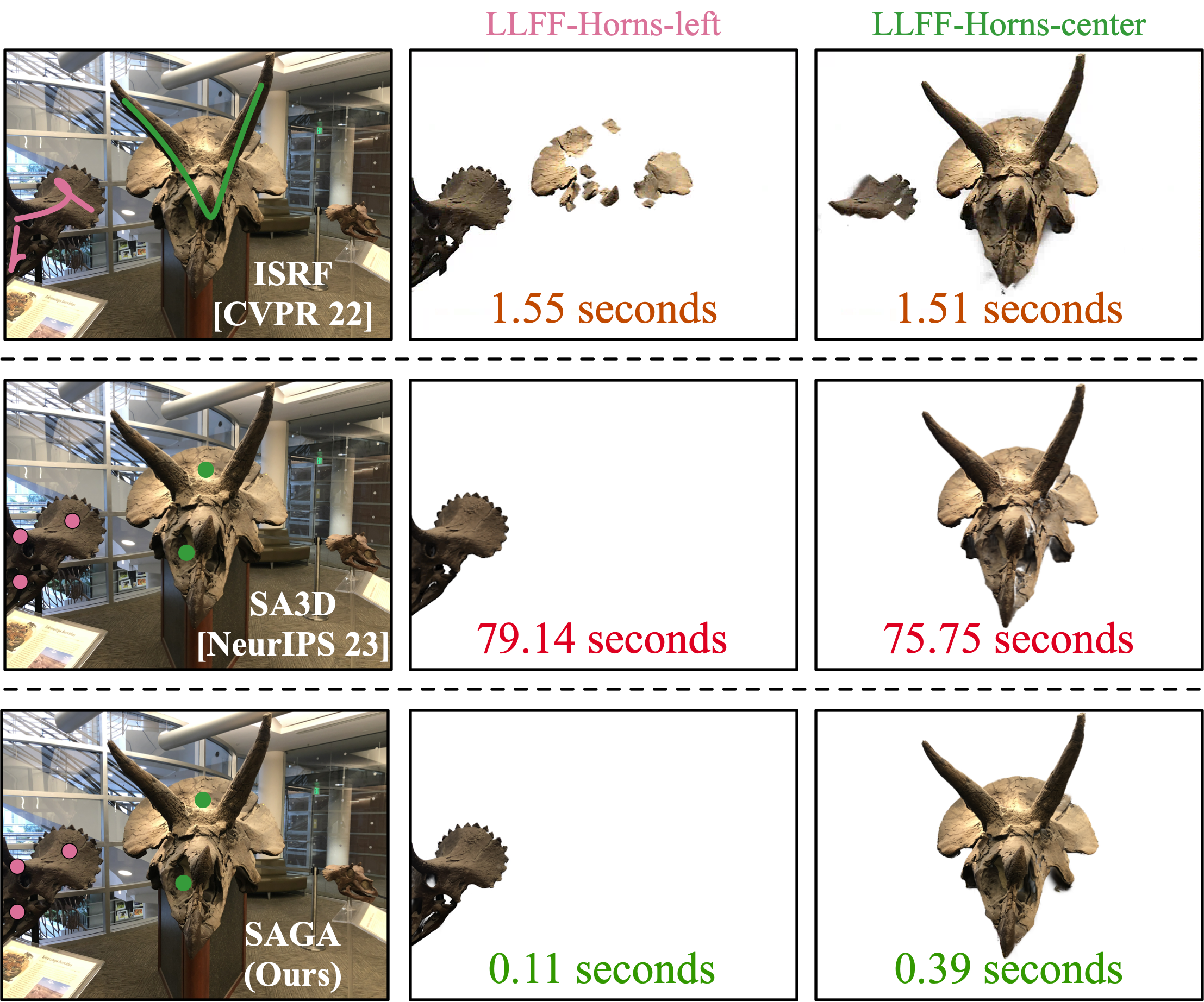
Figure 1: SAGA is a novel interactive 3D segmentation approach that delivers precise 3D segmentation in milliseconds. Each segmentation result displays the computation time in seconds at the lower part, indicating the duration from the user’s prompt input to the acquisition of the segmentation result.

The above discussion reveals the dilemma of currently existing paradigms in achieving both efficiency and accuracy, pointing out two factors that limit the performance of existing paradigms. First, implicit radiance fields employed by previous approaches [13, 5] hinder efficient segmentation: the 3D space must be traversed to retrieve a 3D object. Second, the utilization of the 2D segmentation decoder brings high segmentation quality but low efficiency.

Accordingly, we revisit this task starting from the recent breakthrough in radiance fields: 3D Gaussian Splatting (3DGS) has become a game changer because of its ability in high-quality and real-time rendering. It adopts a set of 3D colored Gaussians to represent the 3D scene. The mean of these Gaussians denotes their position in the 3D space thus 3DGS can be seen as a kind of point cloud, which helps bypass the extensive processing of vast, often empty, 3D spaces and provides abundant explicit 3D prior. With this point cloud-like structure, 3DGS not only realizes efficient rendering but also becomes as an ideal candidate for segmentation tasks.

On the basis of 3DGS, we propose to distill the fine-grained segmentation ability of a 2D segmentation foundation model (i.e., the Segment Anything Model) into the 3D Gaussians. This strategy marks a departure from previous methods that focuses on lifting 2D visual features to 3D and enables fine-grained 3D segmentation. Moreover, it avoids the time-consuming multiple forwarding of the 2D segmentation model during inference. The distillation is achieved by training 3D features for Gaussians based on automatically extracted masks with the Segment Anything Model (SAM) [23]. During inference, a set of queries are generated with input prompts, which, are then used to retrieve the expected Gaussians through efficient feature matching.

Named as Segment Any 3D GAussians (SAGA), our approach can achieve fine-grained 3D segmentation in milliseconds and support various kinds of prompts including points, scribbles and masks. Evaluation on existing benchmarks demonstrates the segmentation quality of SAGA is on par with previous state-of-the-art.

As the first attempt of interactive segmentation in 3D Gaussians, SAGA is versatile, accommodating a range of prompt types, including masks, points, and scribbles. Our evaluation on existing benchmarks demonstrates that SAGA performs on par with the state-of-the-art. Notably, the training of Gaussian features typically concludes within merely 5-10 minutes. Subsequently, the segmentation of most target objects can be completed in milliseconds, achieving nearly $1000\times$ acceleration.

2 Related Work

Promptable 2D segmentation

Inspired by natural language processing and recent computer vision progress, Kirillov et al. [23] proposed the task of promptable segmentation. The goal of this task is to return segmentation masks given input prompts that specify the segmentation target in an image. To solve this problem, they present the Segment Anything Model (SAM), a revolutionary segmentation foundation model. An analogous model to SAM is SEEM [55], which also exhibits impressive open-vocabulary segmentation capabilities. Before them, the most closely related task to promptable 2D segmentation is the interactive image segmentation, which have been explored by many studies [3, 14, 15, 41, 7, 43, 29].

Lifting 2D Vision Foundation Models to 3D

Recently, 2D vision foundation models have experienced robust growth. In contrast, 3D vision foundation models have not seen similar development, primarily due to the scarcity of data. Acquiring and annotating 3D data is significantly more challenging than its 2D counterpart. To tackle this problem, researchers attempted to lift 2D foundation models to 3D [22, 38, 8, 16, 53, 28, 51, 20]. A noteworthy attempt is LERF [22], which trains a feature field of the Vision-Language Model (i.e., CLIP [39]) together with the radiance field. Such paradigm helps locating objects in radiance fields based on language prompts but falls short in precise 3D segmentation, especially when faced with multiple objects of similar semantics. The remaining methods mainly focus on point clouds. By associating the 3D point cloud with 2D multi-view images with the help of camera poses, the extracted features by 2D foundation models can be projected to the 3D point cloud. Such integration is similar to LERF but incurs a higher data acquisition cost compared to radiance field-based methods.

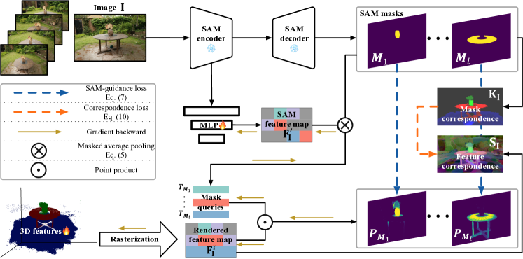
Figure 2: Overall pipeline of SAGA. Given a pre-trained 3DGS model and its training set, we attach a low-dimensional 3D feature to each Gaussian in the model. For every image within the training set, we employ SAM to extract 2D features and a set of masks. Then we render 2D feature maps through the differentiable rasterization and train the attached features with two losses: i.e., the SAM-guidance loss (Eq. 7) and the correspondence loss (Eq. 10). The former adopts SAM features to guide the 3D features to learn 3D segmentation from the ambiguous 2D masks. The latter distills the point-wise correspondence derived from the masks to enhance feature compactness.

3D Segmentation in Radiance Fields

Inspired by the success of radiance fields [32, 45, 6, 1, 34, 18, 11, 49, 27, 10, 50], numerous studies have explored 3D segmentation within them. Zhi et al. [54] proposes Semantic-NeRF, which demonstrates the potential of Neural Radiance Field (NeRF) in semantic propagation and refinement. NVOS [40] introduces an interactive approach to select 3D objects from NeRF by training a lightweight multi-layer perception (MLP) using custom-designed 3D features. By using 2D self-supervised models, e.g. N3F [47], DFF [25], LERF [22] and ISRF [13], aim to lift 2D visual features to 3D by training additional feature fields that can output 2D feature maps imitating the original 2D features in different views. NeRF-SOS [9] distills the 2D feature similarities into 3D features with a correspondence distillation loss [17]. In these 2D visual feature-based approaches, 3D segmentation can be achieved by comparing the 3D features embedded in the feature field, which appears to be efficient. However, since the information embedded in the high-dimensional visual features cannot be fully exploited when relying solely on Euclidean or cosine distances, the segmentation quality of such methods is limited. There are also some other instance segmentation and semantic segmentation approaches [44, 35, 52, 30, 19, 2, 12, 48] combined with radiance fields.

Two most closely related approach to our SAGA is ISRF [13] and SA3D [5]. The former follows the paradigm of training a feature field to imitate multi-view 2D 2D visual features. Thus it struggles with distinguishing different objects (especially parts of object) with similar semantics. The latter iteratively queries SAM to get 2D segmentation results and projecting them onto mask grids for 3D segmentation. Though good segmentation quality, its complex segmentation pipeline leads to high time consumption and inhibits the interaction with users. Compared with them, SAGA can handle multi-granularity 3D segmentation within milliseconds and achieve a better trade-off between the segmentation quality and efficiency.

3 Methodology

3.1 Preliminaries

3D Gaussian Splatting (3DGS)

As a recent advancement of radiance fields, 3DGS [21] uses trainable 3D Gaussians to represent the 3D scene and proposes an efficient differentiable rasterization algorithm for rendering and training. Given a training dataset $\mathcal{I}$ of multi-view 2D images with camera poses, 3DGS learns a set of 3D colored Gaussians $\mathcal{G}=\{\mathbf{g}_{1},\mathbf{g}_{2},...,\mathbf{g}_{N}\}$, where $N$ denotes the number of 3D Gaussians in the scene. The mean of each Gaussian represents its position in the 3D space and the covariance represents the scale. Thus 3DGS can be regarded as a kind of point cloud. Given a specific camera pose, 3DGS projects the 3D Gaussians to 2D and then computes the color $\mathbf{C}$ of a pixel by blending a set of ordered Gaussians $\mathcal{N}$ overlapping the pixel:

$$\mathbf{C}=\sum_{i\in\mathcal{N}}\mathbf{c}_{i}\alpha_{i}\prod_{j=1}^{i-1}(1-\alpha_{j}),$$ (1)

where $\mathbf{c}_{i}$ is the color of each Gaussian and $\alpha_{i}$ is given by evaluating a 2D Gaussian with covariance $\Sigma$ multiplied with a learned per-Gaussian opacity. From Eq. 1 we can learn the linearity of the rasterization process: the color of a rendered pixel is the weighted sum of the involved Gaussians. In our framework, such characteristic ensures the alignment of 3D features with the 2D rendered features.

Segment Anything Model (SAM)

SAM [23] takes an image $\mathbf{I}$ and a set of prompts $\mathcal{P}$ as input, and outputs the corresponding 2D segmentation mask $\mathbf{M}$, i.e.,

$$\mathbf{M}=\text{SAM}(\mathbf{I},\mathcal{P}).$$ (2)

3.2 Overall Pipeline

As shown in Fig. 2, given a pre-trained 3DGS model $\mathcal{G}$ and its training set $\mathcal{I}$, we first employ the SAM encoder to extract a 2D feature map $\mathbf{F}_{\mathbf{I}}^{\text{SAM}}\in\mathbb{R}^{C^{\text{SAM}}\times H\times W}$ and a set of multi-granularity masks $\mathcal{M}_{\mathbf{I}}^{\text{SAM}}$ for each image $\mathbf{I}\in\mathbb{R}^{H\times W}$ in $\mathcal{I}$. Then we train a low-dimensional feature $\mathbf{f_{\mathbf{g}}}\in\mathbb{R}^{C}$ for each Gaussian $\mathbf{g}$ in $\mathcal{G}$ based on the extracted masks to aggregate the cross-view consistent multi-granularity segmentation information ($C$ denotes the feature dimension and is set to 32 in default). This is achieved by a carefully designed SAM-guidance loss. To further enhance the feature compactness, we derive point-wise correspondences from extracted masks and distills them into the features (i.e., the correspondence loss).

In the inference stage, for a specific view with camera pose $v$, a set of queries $\mathcal{Q}$ are generated based on the input prompts $\mathcal{P}$. Then these queries are used to retrieve the 3D Gaussians of the corresponding target by efficient feature matching with the learned features. Additionally, we also introduce an efficient post-processing operation that utilizes the strong 3D prior provided by the point cloud-like structure of 3DGS to refine the retrieved 3D Gaussians.

3.3 Training Features for Gaussians

Given a training image $\mathbf{I}$ with its specific camera pose $v$, we first render the corresponding feature map according to the pre-trained 3DGS model $\mathcal{G}$. Similar to Eq. 1, the rendered feature $\mathbf{F}^{r}_{\mathbf{I},p}$ of a pixel $p$ is computed as:

$$\mathbf{F}^{r}_{\mathbf{I},p}=\sum_{i\in\mathcal{N}}\mathbf{f}_{i}\alpha_{i}\prod_{j=1}^{i-1}(1-\alpha_{j}),$$ (3)

where $\mathcal{N}$ is the ordered set of Gaussians overlapping the pixel. During the training phase, we freeze all other attributes of the 3D Gaussians $\mathcal{G}$ (e.g., mean, covariance and opacity) except the newly attached features.

SAM-guidance Loss

The automatically extracted 2D masks $\mathcal{M}_{\mathbf{I}}$ via SAM are complex and confusing (i.e., a point in the 3D space may be segmented as different objects / parts on different views). Such ambiguous supervision signal poses a great challenge to training 3D features from scratch. To tackle this problem, we propose to use the features generated by SAM for guidance. As shown in Fig. 2, we first adopt an MLP $\varphi$ to project the SAM features to the same low-dimensional space as the 3D features:

$$\mathbf{F}^{\prime}_{\mathbf{I}}=\varphi(\mathbf{F}^{\text{SAM}}_{\mathbf{I}}).$$ (4)

Then for each extracted mask $\mathbf{M}$ in $\mathcal{M}_{\mathbf{I}}^{\text{SAM}}$ we obtain a corresponding query $\mathbf{T}_{\mathbf{M}}\in\mathbb{R}^{C}$ with a masked average pooling operation:

$$\mathbf{T}_{\mathbf{M}}=\frac{1}{||\mathbf{M}||_{1}}\sum_{p=1}^{HW}\mathbbm{1}(\mathbf{M}_{p}=1)\mathbf{F}^{\prime}_{\mathbf{I},p},$$ (5)

where $\mathbbm{1}$ denotes the indicator function. Then $\mathbf{T}_{\mathbf{M}}$ is used to segment the rendered feature map $\mathbf{F}^{r}_{\mathbf{I}}$ through a softmaxed point product:

$$\mathbf{P}_{\mathbf{M}}=\sigma(\mathbf{T}_{\mathbf{M}}\cdot\mathbf{F}^{r}_{\mathbf{I}}),$$ (6)

where $\sigma$ denotes the element-wise sigmoid function. The SAM-guidance loss is defined as the binary cross entropy between the segmentation result $\mathbf{P}_{\mathbf{M}}$ and the corresponding SAM extracted mask $\mathbf{M}$:

$$\mathcal{L}_{\text{SAM}}= -\sum_{\mathbf{I}\in\mathcal{I}}\sum_{\mathbf{M}\in\mathcal{M}_{\mathbf{I}}}\sum_{p}^{HW}[\mathbf{M}_{p}\log\mathbf{P}_{\mathbf{M},p}$$ (7)

$$+(1-\mathbf{M}_{p})\log(1-\mathbf{P}_{\mathbf{M},p})].$$

Correspondence Loss

In practice, we find the learned features with the SAM-guidance loss are not compact enough, which degrades the segmentation quality of various kinds of prompts (refer to the ablation study in Sec. 4 for more details). Inspired by previous contrastive correspondence distillation methods [9, 17], we introduce the correspondence loss to tackle the problem.

As mentioned before, for each image $\mathbf{I}$ with height $H$ and width $W$ in the training set $\mathcal{I}$, a set of masks $\mathcal{M}_{\mathbf{I}}$ are extracted with SAM. Considering two pixels $p_{1},p_{2}$ in $\mathbf{I}$, they may belong to many masks in $\mathcal{M}_{\mathbf{I}}$. Let $\mathcal{M}_{\mathbf{I}}^{p_{1}},\mathcal{M}_{\mathbf{I}}^{p_{2}}$ denote the masks that $p_{1},p_{2}$ belong to respectively. Intuitively, if the intersection over union of the two sets is larger, the two pixels should share more similar features. Thus the mask correspondence $\mathbf{K}_{\mathbf{I}}(p_{1},p_{2})$ is defined as:

$$\mathbf{K}_{\mathbf{I}}(p_{1},p_{2})=\frac{|\mathcal{M}_{\mathbf{I}}^{p_{1}}\cap\mathcal{M}_{\mathbf{I}}^{p_{2}}|}{|\mathcal{M}_{\mathbf{I}}^{p_{1}}\cup\mathcal{M}_{\mathbf{I}}^{p_{2}}|}.$$ (8)

The feature correspondence $\mathbf{S}_{\mathbf{I}}(p_{1},p_{2})$ between two pixels $p_{1},p_{2}$ is defined as the cosine similarity between their rendered features:

$$\mathbf{S}_{\mathbf{I}}(p_{1},p_{2})=<\mathbf{F}^{r}_{\mathbf{I},p_{1}},\mathbf{F}^{r}_{\mathbf{I},p_{2}}>,$$ (9)

then the correspondence loss is defined as:

$$\mathcal{L}_{\text{corr}}=-\sum_{\mathbf{I}\in\mathcal{I}}\sum_{p_{1}}^{HW}\sum_{p_{2}}^{HW}\mathbf{K}_{\mathbf{I}}(p_{1},p_{2})\mathbf{S}_{\mathbf{I}}(p_{1},p_{2}).$$ (10)

If two pixels never belong to the same segment, we reduce their feature similarity by setting the 0-valued entries in $\mathbf{K}_{\mathbf{I}}$ to $-1$.

With the two components of the SAM-guidance loss (Eq. 7) and the correspondence loss (Eq. 10), the final loss of SAGA is:

$$\mathcal{L}=\mathcal{L}_{\text{SAM}}+\lambda\mathcal{L}_{\text{corr}},$$ (11)

where $\lambda$ is a hyper-parameter for balancing the two loss terms (set to 1 in default).

3.4 Inference

Though the training is performed on the rendered feature maps, the linearity of the rasterization operation (shown in Eq. 3) ensures that the features in the 3D space are aligned with the rendered features on the image plane. Thus, the segmentation of the 3D Gaussians can be achieved with 2D-rendered features. This characteristic endows SAGA with the compatibility with different kinds of prompts including points, scribbles and masks. Moreover, we introduce an efficient post-processing algorithm (Sec. 3.5) based on the 3D prior provided by 3DGS.

Point Prompt

With a rendered feature map $\mathbf{F}^{r}_{v}$ for a specific view $v$, we generate queries for positive points and negative points by directly retrieving their corresponding features on $\mathbf{F}^{r}_{v}$. Let $\mathcal{Q}^{p}_{v}$ and $\mathcal{Q}^{n}_{v}$ denote the $N_{p}$ positive queries and $N_{n}$ negative queries respectively. For a 3D Gaussian $\mathbf{g}$, its positive score $S^{p}_{\mathbf{g}}$ is defined as the maximum cosine similarity between its feature $\mathbf{f}_{\mathbf{g}}$ and the positive queries $\mathcal{Q}^{p}_{v}$, i.e., $\max\{<\mathbf{f}_{\mathbf{g}},\mathbf{Q}^{p}>|\mathbf{Q}^{p}\in\mathcal{Q}^{p}_{v}\}$. Similarly, the negative score $S^{n}_{\mathbf{g}}$ is defined as $\max\{<\mathbf{f}_{\mathbf{g}},\mathbf{Q}^{n}>|\mathbf{Q}^{n}\in\mathcal{Q}^{n}_{v}\}$. The 3D Gaussian belongs to the target $\mathcal{G}^{t}$ only if $S^{p}_{\mathbf{g}}>S^{n}_{\mathbf{g}}$.

To further filter out noisy Gaussians, an adaptive threshold $\tau$ is set to the positive score, i.e., $\mathbf{g}\in\mathcal{G}^{t}$ only if $S^{p}_{\mathbf{g}}>\tau$. $\tau$ is set as the mean of the maximum positive scores. Note that such filtering may cause many false negatives, but can be solved by the post-processing introduced in Sec. 3.5.

Mask And Scribble Prompts

Simply treating the dense prompts as multiple points will lead to unaffordable GPU memory overhead. Thus we employ the K-means algorithm to extract some positive queries $\mathcal{Q}^{p}_{v}$ and negative queries $\mathcal{Q}^{n}_{v}$ from the dense prompts. The number of clusters of K-means is set to 5 empirically, but is adjustable according to the complexity of the target object.

SAM-based Prompt

The previous prompts are obtained from rendered feature maps. With the SAM-guidance loss, we can directly use the low-dimensional SAM features $\mathbf{F}^{\prime}_{v}$ for generating queries. The input prompts are first fed into SAM for generating accurate 2D segmentation result $\mathbf{M}^{\text{ref}}_{v}$. With this 2D mask, we first obtain a query $\mathbf{Q}^{\text{mask}}$ with the masked average pooling and use this query to segment the 2D rendered feature map $\mathbf{F}^{r}_{v}$ to get a temporary 2D segmentation mask $\mathbf{M}^{\text{temp}}_{v}$, which is then compared with $\mathbf{M}^{\text{ref}}_{v}$. If the intersecting region of $\mathbf{M}^{\text{temp}}_{v}$ and $\mathbf{M}^{\text{ref}}_{v}$ occupies a large proportion (90%, by default) of $\mathbf{M}^{\text{ref}}_{v}$, $\mathbf{Q}^{\text{mask}}_{v}$ is accepted as the query. Otherwise, we use the K-means algorithm to extract another set of queries $\mathcal{Q}^{\text{kmeans}}_{v}$ from the low-dimensional SAM features $\mathbf{F}^{\prime}_{v}$ within the mask. We adopt such strategy because that the segmentation target may contain many components, which cannot be captured by simply applying the masked average pooling.

After obtaining the query set $\mathcal{Q}^{\text{SAM}}_{v}=\{\mathbf{Q}^{\text{mask}}_{v}\}$ or $\mathcal{Q}^{\text{SAM}}_{v}=\mathcal{Q}^{\text{kmeans}}_{v}$, the subsequent process is almost the same as the former prompt approaches. We use the point product instead of the cosine similarity as the metric for segmentation to align with the SAM-guidance loss. For a 3D Gaussian $\mathbf{g}$, its positive score $S^{p}_{\mathbf{g}}$ is defined as the maximum point product computed with these queries:

$$S^{p}_{\mathbf{g}}=\max\{\mathbf{f}_{\mathbf{g}}\cdot\mathbf{Q}|\mathbf{Q}\in\mathcal{Q}^{\text{SAM}}_{v}\}.$$ (12)

The 3D Gaussian $\mathbf{g}$ belongs to the segmentation target $\mathcal{G}^{t}$ if its positive score is greater than another adaptive threshold $\tau^{\text{SAM}}$, which is the sum of the mean and the standard deviation of all scores $\mathcal{S}_{\mathcal{G}}=\{S^{p}_{\mathbf{g}}|\mathbf{g}\in\mathcal{G}\}$.

3.5 3D Prior Based Post-processing

The initial segmentation $\mathcal{G}^{t}$ of the 3D Gaussians exhibits two primary problems: (i) the presence of superfluous noisy Gaussians and (ii) the omission of certain Gaussians integral to the target object. To tackle the problem, we utilize traditional point cloud segmentation techniques [36, 37, 42], including statistical filtering and region growing. For segmentation based on point and scribble prompts, statistical filtering is employed to filter out noisy Gaussians. For mask prompts and SAM-based prompts, the 2D mask is projected onto $\mathcal{G}^{t}$ to get a set of validated Gaussians and projected onto $\mathcal{G}$ to exclude unwanted Gaussians. The resulting validated Gaussians serve as the seed for the region-growing algorithm. Finally, a ball query-based region growing method is applied to retrieve all required Gaussians of the target from the original model $\mathcal{G}$.

Statistical Filtering

The distance between two Gaussians can indicate whether they belong to the same target. Statistical filtering begins by employing the K-Nearest Neighbors (KNN) algorithm to calculate the average distance of the nearest $\sqrt{|\mathcal{G}^{t}|}$ Gaussians for each Gaussian within the segmentation result $\mathcal{G}^{t}$. Subsequently, we compute the mean ($\mu$) and standard deviation ($\sigma$) of these average distances across all Gaussians in $\mathcal{G}^{t}$. We then remove Gaussians with an average distance exceeding $\mu+\sigma$ to get $\mathcal{G}^{t\prime}$.

Region Growing Based Filtering

The 2D mask from mask prompt or SAM-based prompt can serve as a prior for accurately localizing the target. Initially, we project the mask onto the segmented Gaussians $\mathcal{G}^{t}$, yielding a subset of validated Gaussians, denoted as $\mathcal{G}^{c}$. Subsequently, for each Gaussian $\mathbf{g}$ within $\mathcal{G}^{c}$, we compute its Euclidean distance $d_{\mathbf{g}}$ to its closest neighbor in the same subset:

$$d_{\mathbf{g}}^{\mathcal{G}^{c}}=\min\{D(\mathbf{g},\mathbf{g}^{\prime})|\mathbf{g}^{\prime}\in\mathcal{G}^{c}\},$$ (13)

where $D(\cdot,\cdot)$ denotes the Euclidean distance. Then we iteratively incorporate neighboring Gaussians in $\mathcal{G}^{t}$ whose distances are less than the maximum nearest neighbor distance observed in the set $\mathcal{G}^{c}$, formalized as $\max\{d_{\mathbf{g}}^{\mathcal{G}^{c}}|\mathbf{g}\in\mathcal{G}^{c}\}$. After the region growing converging, where no new Gaussians in $\mathcal{G}^{f}$ meet the criteria, we get the filtered segmentation result $\mathcal{G}^{t\prime}$.

Note that though the point prompt and scribble prompt can also roughly locate the target, region growing based on them is time-consuming. Thus we only apply the region growing based filtering when a mask is available.

Ball Query Based Growing

The filtered segmentation output $\mathcal{G}^{t\prime}$ may not contain all Gaussians belong to the target. To address this problem, we utilize a ball query algorithm to retrieve all required Gaussians from all Gaussians $\mathcal{G}$. Concretely, this is achieved by checking spherical neighborhoods with a radius $r$, centered at each Gaussian in $\mathcal{G}^{t\prime}$. Gaussians that are located within these spherical boundaries in $\mathcal{G}$ are then aggregated into the final segmentation result $\mathcal{G}^{s}$. The radius $r$ is set to be the maximum nearest neighbor distance in $\mathcal{G}^{t\prime}$, i.e., $r=\max\{d_{\mathbf{g}}^{\mathcal{G}^{t\prime}}|\mathbf{g}\in\mathcal{G}^{t\prime}\}$.

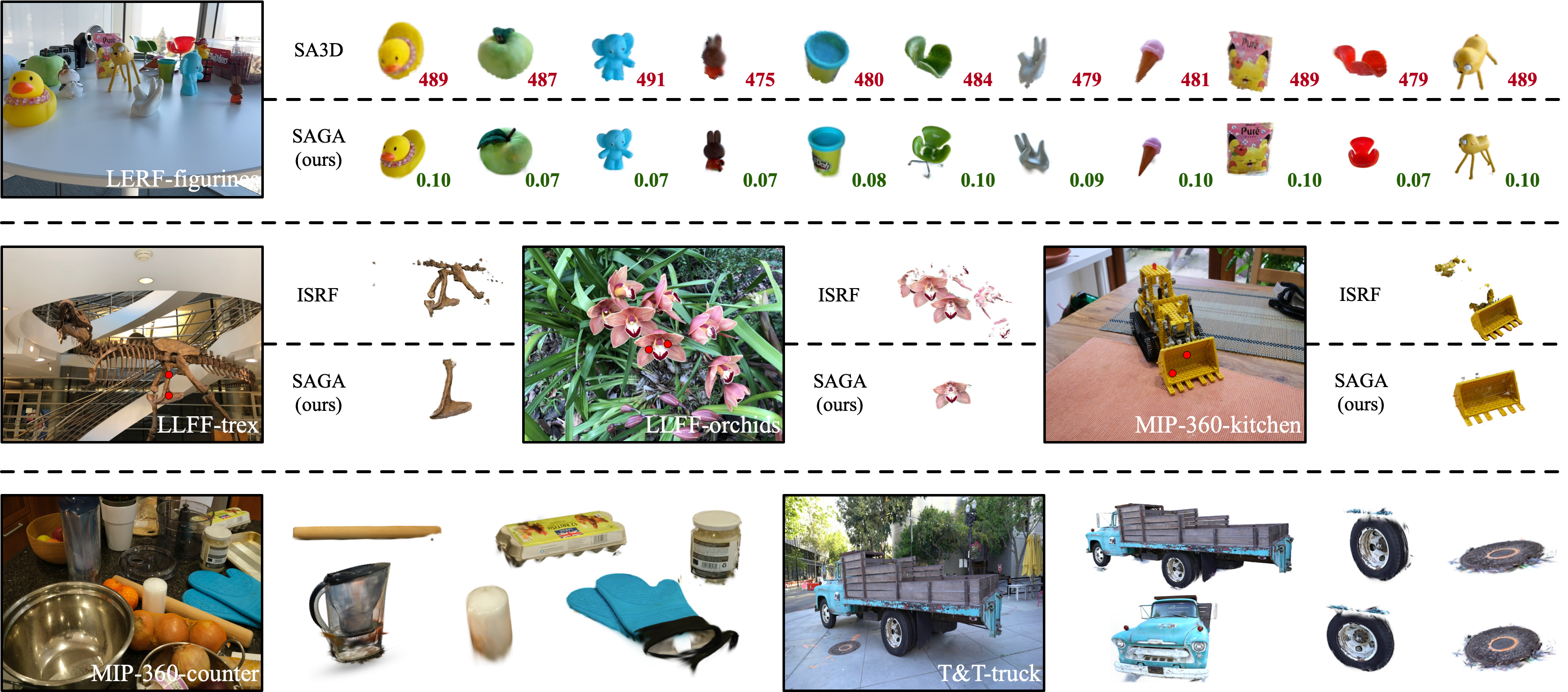
Figure 3: Qualitative results of SAGA. Compared with SA3D, SAGA can achieve similar performance within one thousandth of the time. Compared with ISRF, SAGA can distinguish object with similar semantics and realize part segmentation. Furthermore, thanks to the efficient 3D Gaussian representation, the rendering quality of the segmented object is better than previous SOTA SA3D and ISRF.

4 Experiments

4.1 Datasets

For quantitative experiments, we use the Neural Volumetric Object Selection (NVOS) [40], SPIn-NeRF [33] datasets. The NVOS [40] dataset is based on the LLFF dataset [31], which includes several forward-facing scenes. For each scene, the NVOS dataset provides a reference view with scribbles and a target view with 2D segmentation masks annotated. Similarly, the SPIn-NeRF [33] dataset also annotates some data manually based on widely-used NeRF datasets [31, 32, 26, 24, 11]. Futhermore, we also use SA3D to annotate some objects in the LERF-figurines scene to demonstrate the better trade-off of efficiency and segmentation quality achieved by SAGA. For qualitative analysis, we use the LLFF [31] dataset, the MIP-360 dataset [1], the T&T dataset [24] and the LERF dataset [22].

4.2 Quantitative Results

Table 1: Quantitative results on NVOS.

Method	mIoU (%)	mAcc (%)
Graph-cut (3D) [41, 40]	39.4	73.6
NVOS [40]	70.1	92.0
ISRF [13]	83.8	96.4
SGISRF [46]	86.4	97.6
SA3D [5]	90.3	98.2
SAGA (ours)	90.9	98.3

NVOS

We follow SA3D [5] to process the scribbles provided by the NVOS dataset to meet the requirements of SAM. As shown in Table 1, SAGA is on par with previous SOTA SA3D and significantly outperforms previous feature imitation-based approach (ISRF and SGISRF), which demonstrates its fine-grained segmentation ability.

SPIn-NeRF

We follow SPIn-NeRF [33] to conduct label propagation for evaluation, which specifies a view with its 2D ground-truth mask and propagate this mask to other views to check the mask accuracy. This operation can be seen as a kind of mask prompt. The results are shown in Table 2. MVSeg adopts the video segmentation approach [4] to segment the multi-view images and SA3D automatically queries 2D segmentation foundation model for rendered images on the training views. Both of them need to forward a 2D segmentation model for many times. Remarkably, SAGA shows comparable performance with them in nearly one-thousandth of the time. Note that the slight degradation is caused by the sub-optimal geometry learned by 3DGS. Please refer to Sec. 4.3 for more details.

Table 2: Quantitative results on the SPIn-NeRF dataset. ‘Singe view’ denotes projecting the 2D segmentation result to 3D simply, thus we omit its time consumption.

Method	mIoU (%)	mAcc (%)	Time
Single view [5]	74.6	95.5	-
MVSeg [33]	90.9	98.9	3-6 minutes
SA3D [5]	92.4	98.9	2-10 minutes
SAGA (ours)	88.0	98.5	0.08-0.9 seconds

Comparison with SA3D

To further demonstrate the effectiveness of SAGA, we compare the segmentation time consumption and the quality with SA3D. We run SA3D based on the LERF-figurines scene to get a set of annotations for many objects. Subsequently we use SAGA to segment the same objects and check the IoU and time cost for each object. The results are shown in Table 3, We also provide visualization results for comparison with SA3D, please refer to Sec. 4.3 for more details. It is noteworthy to mention that limited by the huge GPU memory cost of SA3D, the training resolution of SAGA is much higher. This indicates that SAGA can get 3D assets with higher quality in much less time. Even considering the training time (about 10 minutes per scene), the average segmentation time for each object of SAGA is much less than SA3D.

Table 3: Comparison with SA3D on the LERF-figurines. Since the annotation is generated by SA3D, its mIoU is omitted.

Method	Mean Time Cost (s / object)	mIoU (%)
SA3D	484	-
SAGA	0.09	93.82

4.3 Qualitative Results

We begin by establishing that SAGA attains a segmentation accuracy on par with the prior SOTA, SA3D, while significantly reducing time cost. Subsequently, we demonstrate the enhanced performance of SAGA over ISRF, in both part and object segmentation tasks. Results are shown in Fig. 3.

The first row shows the segmentation results of SA3D and SAGA on the LERF-figurines scene, with segmentation times annotated in the lower right of each segmented object. The second row compares SAGA with ISRF, which trains a feature field by imitating the 2D features extracted by a self-supervised vision transformer (e.g., DINO [4]). ISRF struggles to differentiate between objects of similar semantics, like parts of the T-Rex skeleton. In contrast, SAGA distills the knowledge embedded in the SAM decoder into the feature field, thereby adeptly managing such complexities. Additional segmentation results for the MIP-360-counter [1] and T&T-truck [24] scenes are presented in the third row. It’s important to note the noise present at the periphery of the segmented targets. This is attributed to the inherent properties of 3D Gaussians, where a certain Gaussian intersect multiple objects, particularly at the boundaries where different objects meet.

Failure Cases

In Table 2, SAGA exhibits sub-optimal performance compared to the previous state-of-the-art methods. This is because of a segmentation failure of the LLFF-room scene, which reveals a limitation of SAGA. We show the mean of the colored Gaussians in Fig. 4, which can be seen as a kind of point cloud. SAGA is susceptible to inadequate geometric reconstruction of the 3DGS model. As marked by the red boxes, the Gaussians of the table is notably sparse, where the Gaussians representing the table surface are floating beneath the actual surface. Even worse, the Gaussians from the chair are in close proximity to those of the table. These issues not only impede the learning of discriminative 3D features but also compromise the efficacy of the post-processing. We believe that enhancing the geometric fidelity of the 3DGS model can ameliorate this issue.

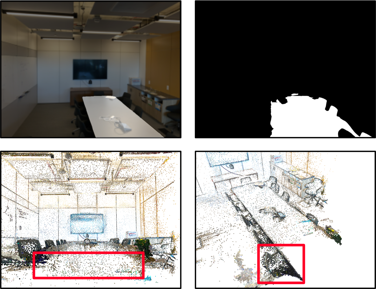
Figure 4: A failure case of SAGA. The upper-right part shows the segmentation result, and the lower part shows the mean of Gaussians of the 3DGS model. The failure is caused by the incorrect geometric structure of the learned Gaussians by 3DGS.

4.4 Ablation Study

Loss Terms

Our loss function comprises two key components: 1) SAM-guidance loss and 2) Correspondence loss. We demonstrate their efficacy quantitatively and qualitatively. As shown in Table 4, the absence of SAM-guidance loss significantly hinders the performance of SAGA in complex scenes, such as LLFF-fern, due to the ambiguous nature of the segmentation targets. Furthermore, as indicated in Fig. 5, excluding the correspondence loss leads to less compact 3D features. This affects the effectiveness of various kinds of prompts and makes the SAM-based prompt as the sole effective approach.

Table 4: Effect of different loss terms on NVOS dataset. “Corr.” denotes the correspondence loss. “S-guidance” stands for the SAM-guidance loss. The absence of the SAM-guidance loss leads to significant degradation in segmentation performance, attributed to the complexity of the training target.

Scene	SAGA	w/o Corr.	w/o S-guidance
Fern	80.45	75.93	41.96
Flower	95.51	91.57	81.50
Fortress	96.39	94.53	77.48
Horns-center	94.65	95.94	85.14
Horns-left	92.06	79.83	91.62
Leaves	90.58	91.17	88.18
Orchids	94.47	91.02	87.97
Trex	83.29	81.08	84.61
mean	90.93	87.63	79.81

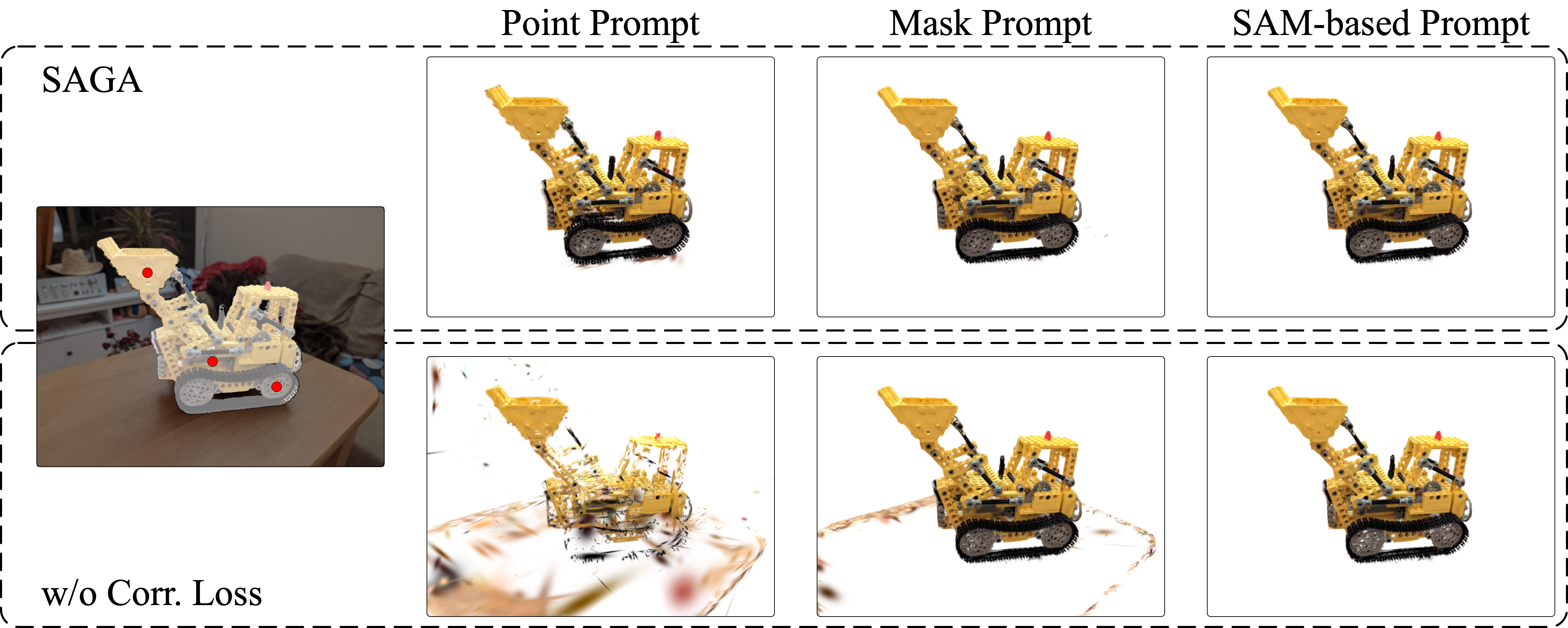
Figure 5: Ablation on the effect of the correspondence loss. The point prompt and mask prompt are annotated on the original image. Without this loss term, the learned features are not compact enough, which greatly impedes point prompt-based segmentation and mask prompt-based segmentation.

Post-processing

As shown in Fig. 6, without the post-processing there are some noisy Gaussians in the segmentation result and the segmentation target (the flowers) seems translucent due to the missing Gaussians.

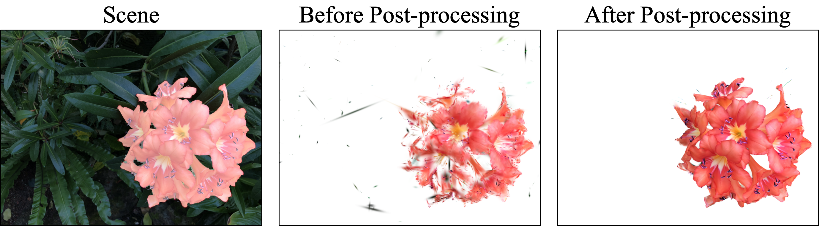
Figure 6: Ablation on the effect of the post-processing. The segmentation target is highlighted. Without the post-processing, the segmentation result is noisy and incomplete.

Computation Consumption

We analyse the time cost of SAGA based on the T&T-truck scene [24] and the LERF-figurines scene [22]. The segmentation target for the former is the truck and for the latter is the green apple on the table. Both of them can be found in Fig. 3. As shown in Table 5, for large targets, the primary computation lies in post-processing. In contrast, for the smaller target, the time cost of Gaussians retrieving becomes the main consumption, which depends on the complexity of the scene.

Table 5: Computation consumption analysis. The number of Gaussians indicates the scale of the scene and the corresponding segmentation target. The computation of SAGA can be split into three phases: Gaussians retrieving, post-process (filtering) and post-process (growing).

Scene	Number of Gaussians		Time Cost (ms)
	Total	Target	Retrieving	P-filtering	P-growing
T&T-truck	2576 K	464 K	53	141	134
LERF-figurines	2188 K	7 K	43	28	14

5 Limitation

SAGA requires training features for 3D Gaussians, which makes it more suitable for scenes with multiple objects to be segmented than object-centric scenes. Besides, the primary limitations of SAGA stem from 3DGS and SAM, which can be summarized as follows:

• The Gaussians learned by 3DGS are ambiguous without any constraint on geometry. A single Gaussian might correspond to multiple objects, complicating the task of accurately segmenting individual objects through feature matching. We believe this issue can be alleviated by future progress in the 3DGS representation.

• The masks automatically extracted by SAM tend to exhibit a certain level of noise as a byproduct of the multi-granularity characteristic. This can be alleviated by adjusting the hyper-parameters involved in automatic mask extraction.

Additionally, it’s important to note that the post-processing step in SAGA is semantic-agnostic, which may bring some false positive points into the segmentation result. We leave this issue as future work.

6 Conclusion

In this paper, we introduce SAGA, a novel interactive 3D segmentation method. As the first attempt of interactive segmentation in 3D Gaussians, SAGA effectively distills knowledge from the Segment Anything Model (SAM) into 3D Gaussians using two carefully designed losses. After training, SAGA allows for rapid, millisecond-level 3D segmentation across various input types like points, scribbles, and masks. Extensive experiments are conducted to demonstrate the efficiency and effectiveness of SAGA.

References

- Barron et al. [2022] Jonathan T. Barron, Ben Mildenhall, Dor Verbin, Pratul P. Srinivasan, and Peter Hedman. Mip-nerf 360: Unbounded anti-aliased neural radiance fields. In CVPR, 2022.
- Bing et al. [2022] Wang Bing, Lu Chen, and Bo Yang. Dm-nerf: 3d scene geometry decomposition and manipulation from 2d images. arXiv preprint arXiv:2208.07227, 2022.
- Boykov and Jolly [2001] Yuri Y Boykov and M-P Jolly. Interactive graph cuts for optimal boundary & region segmentation of objects in nd images. In ICCV, 2001.
- Caron et al. [2021] Mathilde Caron, Hugo Touvron, Ishan Misra, Hervé Jégou, Julien Mairal, Piotr Bojanowski, and Armand Joulin. Emerging properties in self-supervised vision transformers. In ICCV, 2021.
- Cen et al. [2023] Jiazhong Cen, Zanwei Zhou, Jiemin Fang, Chen Yang, Wei Shen, Lingxi Xie, Dongsheng Jiang, Xiaopeng Zhang, and Qi Tian. Segment anything in 3d with nerfs. In NeurIPS, 2023.
- Chen et al. [2022a] Anpei Chen, Zexiang Xu, Andreas Geiger, Jingyi Yu, and Hao Su. Tensorf: Tensorial radiance fields. In ECCV, 2022a.
- Chen et al. [2022b] Xi Chen, Zhiyan Zhao, Yilei Zhang, Manni Duan, Donglian Qi, and Hengshuang Zhao. Focalclick: Towards practical interactive image segmentation. In CVPR, 2022b.
- Ding et al. [2023] Runyu Ding, Jihan Yang, Chuhui Xue, Wenqing Zhang, Song Bai, and Xiaojuan Qi. Pla: Language-driven open-vocabulary 3d scene understanding. In CVPR, 2023.
- Fan et al. [2023] Zhiwen Fan, Peihao Wang, Yifan Jiang, Xinyu Gong, Dejia Xu, and Zhangyang Wang. Nerf-sos: Any-view self-supervised object segmentation on complex scenes. In ICLR, 2023.
- Fang et al. [2022] Jiemin Fang, Taoran Yi, Xinggang Wang, Lingxi Xie, Xiaopeng Zhang, Wenyu Liu, Matthias Nießner, and Qi Tian. Fast dynamic radiance fields with time-aware neural voxels. In SIGGRAPH Asia, 2022.
- Fridovich-Keil et al. [2022] Sara Fridovich-Keil, Alex Yu, Matthew Tancik, Qinhong Chen, Benjamin Recht, and Angjoo Kanazawa. Plenoxels: Radiance fields without neural networks. In CVPR, 2022.
- Fu et al. [2022] Xiao Fu, Shangzhan Zhang, Tianrun Chen, Yichong Lu, Lanyun Zhu, Xiaowei Zhou, Andreas Geiger, and Yiyi Liao. Panoptic nerf: 3d-to-2d label transfer for panoptic urban scene segmentation. In 3DV, 2022.
- Goel et al. [2022] Rahul Goel, Dhawal Sirikonda, Saurabh Saini, and PJ Narayanan. Interactive segmentation of radiance fields. arXiv preprint arXiv:2212.13545, 2022.
- Grady [2006] Leo Grady. Random walks for image segmentation. IEEE Trans. Pattern Anal. Mach. Intell., 2006.
- Gulshan et al. [2010] Varun Gulshan, Carsten Rother, Antonio Criminisi, Andrew Blake, and Andrew Zisserman. Geodesic star convexity for interactive image segmentation. In CVPR, 2010.
- Ha and Song [2022] Huy Ha and Shuran Song. Semantic abstraction: Open-world 3d scene understanding from 2d vision-language models. In CoRL, 2022.
- Hamilton et al. [2022] Mark Hamilton, Zhoutong Zhang, Bharath Hariharan, Noah Snavely, and William T Freeman. Unsupervised semantic segmentation by distilling feature correspondences. In ICLR, 2022.
- Hedman et al. [2021] Peter Hedman, Pratul P. Srinivasan, Ben Mildenhall, Jonathan T. Barron, and Paul E. Debevec. Baking neural radiance fields for real-time view synthesis. In ICCV, 2021.
- Hu et al. [2023] Benran Hu, Junkai Huang, Yichen Liu, Yu-Wing Tai, and Chi-Keung Tang. Instance neural radiance field. arXiv preprint arXiv:2304.04395, 2023.
- Jatavallabhula et al. [2023] Krishna Murthy Jatavallabhula, Alihusein Kuwajerwala, Qiao Gu, Mohd Omama, Tao Chen, Shuang Li, Ganesh Iyer, Soroush Saryazdi, Nikhil Keetha, Ayush Tewari, et al. Conceptfusion: Open-set multimodal 3d mapping. arXiv preprint arXiv:2302.07241, 2023.
- Kerbl et al. [2023] Bernhard Kerbl, Georgios Kopanas, Thomas Leimkühler, and George Drettakis. 3d gaussian splatting for real-time radiance field rendering. ACM Transactions on Graphics (ToG), 2023.
- Kerr et al. [2023] Justin Kerr, Chung Min Kim, Ken Goldberg, Angjoo Kanazawa, and Matthew Tancik. Lerf: Language embedded radiance fields. arXiv preprint arXiv:2303.09553, 2023.
- Kirillov et al. [2023] Alexander Kirillov, Eric Mintun, Nikhila Ravi, Hanzi Mao, Chloe Rolland, Laura Gustafson, Tete Xiao, Spencer Whitehead, Alexander C Berg, Wan-Yen Lo, et al. Segment anything. arXiv preprint arXiv:2304.02643, 2023.
- Knapitsch et al. [2017] Arno Knapitsch, Jaesik Park, Qian-Yi Zhou, and Vladlen Koltun. Tanks and temples: Benchmarking large-scale scene reconstruction. ACM Trans. Graph., 2017.
- Kobayashi et al. [2022] Sosuke Kobayashi, Eiichi Matsumoto, and Vincent Sitzmann. Decomposing nerf for editing via feature field distillation. In NeurIPS, 2022.
- Lin et al. [2022] Yen-Chen Lin, Pete Florence, Jonathan T. Barron, Tsung-Yi Lin, Alberto Rodriguez, and Phillip Isola. Nerf-supervision: Learning dense object descriptors from neural radiance fields. In ICRA, 2022.
- Lindell et al. [2021] David B. Lindell, Julien N. P. Martel, and Gordon Wetzstein. Autoint: Automatic integration for fast neural volume rendering. In CVPR, 2021.
- Liu et al. [2023a] Minghua Liu, Yinhao Zhu, Hong Cai, Shizhong Han, Zhan Ling, Fatih Porikli, and Hao Su. Partslip: Low-shot part segmentation for 3d point clouds via pretrained image-language models. In CVPR, 2023a.
- Liu et al. [2023b] Qin Liu, Zhenlin Xu, Gedas Bertasius, and Marc Niethammer. Simpleclick: Interactive image segmentation with simple vision transformers. In ICCV, 2023b.
- Liu et al. [2022] Xinhang Liu, Jiaben Chen, Huai Yu, Yu-Wing Tai, and Chi-Keung Tang. Unsupervised multi-view object segmentation using radiance field propagation. In NeurIPS, 2022.
- Mildenhall et al. [2019] Ben Mildenhall, Pratul P. Srinivasan, Rodrigo Ortiz Cayon, Nima Khademi Kalantari, Ravi Ramamoorthi, Ren Ng, and Abhishek Kar. Local light field fusion: practical view synthesis with prescriptive sampling guidelines. ACM Trans. Graph., 2019.
- Mildenhall et al. [2020] Ben Mildenhall, Pratul P. Srinivasan, Matthew Tancik, Jonathan T. Barron, Ravi Ramamoorthi, and Ren Ng. Nerf: Representing scenes as neural radiance fields for view synthesis. In ECCV, 2020.
- Mirzaei et al. [2023] Ashkan Mirzaei, Tristan Aumentado-Armstrong, Konstantinos G. Derpanis, Jonathan Kelly, Marcus A. Brubaker, Igor Gilitschenski, and Alex Levinshtein. SPIn-NeRF: Multiview segmentation and perceptual inpainting with neural radiance fields. In CVPR, 2023.
- Müller et al. [2022] Thomas Müller, Alex Evans, Christoph Schied, and Alexander Keller. Instant neural graphics primitives with a multiresolution hash encoding. ACM Trans. Graph., 2022.
- Niemeyer and Geiger [2021] Michael Niemeyer and Andreas Geiger. GIRAFFE: representing scenes as compositional generative neural feature fields. In CVPR, 2021.
- Ning et al. [2009] Xiaojuan Ning, Xiaopeng Zhang, Yinghui Wang, and Marc Jaeger. Segmentation of architecture shape information from 3d point cloud. In VRCAI, 2009.
- Nurunnabi et al. [2012] Abdul Nurunnabi, David Belton, and Geoff West. Robust segmentation in laser scanning 3d point cloud data. In DICTA, 2012.
- Peng et al. [2023] Songyou Peng, Kyle Genova, Chiyu Jiang, Andrea Tagliasacchi, Marc Pollefeys, Thomas Funkhouser, et al. Openscene: 3d scene understanding with open vocabularies. In CVPR, 2023.
- Radford et al. [2021] Alec Radford, Jong Wook Kim, Chris Hallacy, Aditya Ramesh, Gabriel Goh, Sandhini Agarwal, Girish Sastry, Amanda Askell, Pamela Mishkin, Jack Clark, Gretchen Krueger, and Ilya Sutskever. Learning transferable visual models from natural language supervision. In ICML, 2021.
- Ren et al. [2022] Zhongzheng Ren, Aseem Agarwala, Bryan C. Russell, Alexander G. Schwing, and Oliver Wang. Neural volumetric object selection. In CVPR, 2022.
- Rother et al. [2004] Carsten Rother, Vladimir Kolmogorov, and Andrew Blake. ”grabcut”: interactive foreground extraction using iterated graph cuts. ACM Trans. Graph., 2004.
- Rusu and Cousins [2011] Radu Bogdan Rusu and Steve Cousins. 3d is here: Point cloud library (pcl). In ICRA, 2011.
- Sofiiuk et al. [2022] Konstantin Sofiiuk, Ilya A Petrov, and Anton Konushin. Reviving iterative training with mask guidance for interactive segmentation. In ICIP, 2022.
- Stelzner et al. [2021] Karl Stelzner, Kristian Kersting, and Adam R Kosiorek. Decomposing 3d scenes into objects via unsupervised volume segmentation. arXiv preprint arXiv:2104.01148, 2021.
- Sun et al. [2022] Cheng Sun, Min Sun, and Hwann-Tzong Chen. Direct voxel grid optimization: Super-fast convergence for radiance fields reconstruction. In CVPR, 2022.
- Tang et al. [2023] Songlin Tang, Wenjie Pei, Xin Tao, Tanghui Jia, Guangming Lu, and Yu-Wing Tai. Scene-generalizable interactive segmentation of radiance fields. In ACMMM, 2023.
- Tschernezki et al. [2022] Vadim Tschernezki, Iro Laina, Diane Larlus, and Andrea Vedaldi. Neural feature fusion fields: 3d distillation of self-supervised 2d image representations. In 3DV, 2022.
- Vora et al. [2021] Suhani Vora, Noha Radwan, Klaus Greff, Henning Meyer, Kyle Genova, Mehdi SM Sajjadi, Etienne Pot, Andrea Tagliasacchi, and Daniel Duckworth. Nesf: Neural semantic fields for generalizable semantic segmentation of 3d scenes. arXiv preprint arXiv:2111.13260, 2021.
- Wizadwongsa et al. [2021] Suttisak Wizadwongsa, Pakkapon Phongthawee, Jiraphon Yenphraphai, and Supasorn Suwajanakorn. Nex: Real-time view synthesis with neural basis expansion. In CVPR, 2021.
- Wu et al. [2023] Guanjun Wu, Taoran Yi, Jiemin Fang, Lingxi Xie, Xiaopeng Zhang, Wei Wei, Wenyu Liu, Qi Tian, and Wang Xinggang. 4d gaussian splatting for real-time dynamic scene rendering. arXiv preprint arXiv:2310.08528, 2023.
- Yang et al. [2023] Jihan Yang, Runyu Ding, Zhe Wang, and Xiaojuan Qi. Regionplc: Regional point-language contrastive learning for open-world 3d scene understanding. arXiv preprint arXiv:2304.00962, 2023.
- Yu et al. [2022] Hong-Xing Yu, Leonidas J. Guibas, and Jiajun Wu. Unsupervised discovery of object radiance fields. In ICLR, 2022.
- Zhang et al. [2023] Junbo Zhang, Runpei Dong, and Kaisheng Ma. Clip-fo3d: Learning free open-world 3d scene representations from 2d dense clip. arXiv preprint arXiv:2303.04748, 2023.
- Zhi et al. [2021] Shuaifeng Zhi, Tristan Laidlow, Stefan Leutenegger, and Andrew J. Davison. In-place scene labelling and understanding with implicit scene representation. In ICCV, 2021.
- Zou et al. [2023] Xueyan Zou, Jianwei Yang, Hao Zhang, Feng Li, Linjie Li, Jianfeng Gao, and Yong Jae Lee. Segment everything everywhere all at once. arXiv preprint arXiv:2304.06718, 2023.