Refine, Discriminate and Align:
Stealing Encoders via Sample-Wise Prototypes and Multi-Relational Extraction

Abstract

This paper introduces RDA, a pioneering approach designed to address two primary deficiencies prevalent in previous endeavors aiming at stealing pre-trained encoders: (1) suboptimal performances attributed to biased optimization objectives, and (2) elevated query costs stemming from the end-to-end paradigm that necessitates querying the target encoder every epoch. Specifically, we initially Refine the representations of the target encoder for each training sample, thereby establishing a less biased optimization objective before the steal-training phase. This is accomplished via a sample-wise prototype, which consolidates the target encoder’s representations for a given sample’s various perspectives. Demanding exponentially fewer queries compared to the end-to-end approach, prototypes can be instantiated to guide subsequent query-free training. For more potent efficacy, we develop a multi-relational extraction loss that trains the surrogate encoder to Discriminate mismatched embedding-prototype pairs while Aligning those matched ones in terms of both amplitude and angle. In this way, the trained surrogate encoder achieves state-of-the-art results across the board in various downstream datasets with limited queries. Moreover, RDA is shown to be robust to multiple widely-used defenses.

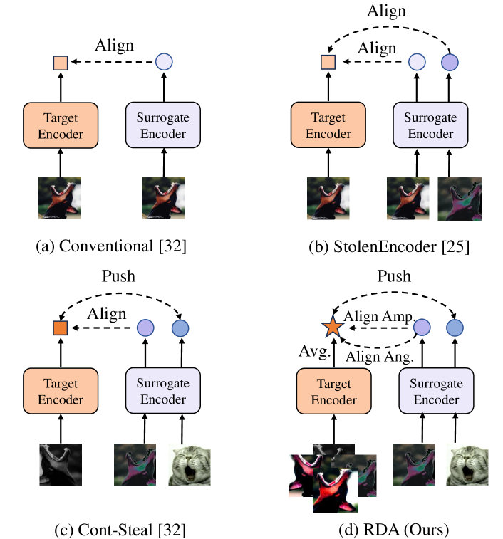
Figure 1: Illustrations of four stealing methods against SSL. The dotted arrows and text beside interpret how each method optimizes the surrogate encoder. Surrogate encoder branches in (a), (b), and (c) involve data augmentations for training. Both (c) and (d) augment each sample before querying the target encoder but adopting different schemes, i.e., end-to-end or generating prototypes.

Introduction

Self-supervised learning (SSL) [30, 1, 2, 3, 39] endows with the capability to harness unlabeled data for pre-training a versatile encoder that applicable to a range of downstream tasks, or even showcasing groundbreaking zero-shot performances, e.g., CLIP [5]. However, SSL typically requires a large volume of data and computation resources to achieve a convincing performance, i.e., high-performance encoders are expensive to train [35]. To safeguard the confidentiality and economic worth of these encoders, entities like OpenAI offer their encoders as a premium service, exclusively unveiling the service API to the public. Users have the privilege of soliciting embeddings for their data, facilitating the training of diverse models tailored for specific downstream tasks. Regrettably, the substantial value of these encoders and their exposure to publicly accessible APIs render them susceptible to model stealing attacks [18, 19, 17].

Given a surrogate dataset, model stealing attacks aim to mimic the outputs of a target model to train either a high-accuracy copy of comparable performance or a high-fidelity copy that can serve as a stepping stone to perform further attacks like adversarial examples [33], membership inference attacks [36, 37], etc. The goal of this paper is to develop an advanced approach that can train a surrogate encoder with competitive performance on downstream tasks by only accessing the target encoder’s output embeddings. Meanwhile, it should require as little cost as possible, which is primarily derived from querying the target encoder.

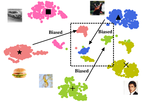
Figure 2: t-SNE of embeddings belonging to five different images generated by an encoder pre-trained on CIFAR10 (KNN Accuracy = 88.31%, tested on CIFAR10), with each image augmented into 500 patches and fed into the encoder. Each black marker represents the mean of the 500 embeddings of a certain image, i.e., its prototype. Among the embeddings of an image’s various augmentations, some can be diverged or even biased. In contrast, each image’s prototype is more distinguishable, i,e., less biased.

We begin with systematically studying existing techniques for stealing pre-trained encoders. Specifically, the conventional method [19] and StolenEncoder [18] are similar, and both only need to query the target encoder once with each sample before the training. The output embedding can be viewed as a “ground truth” or an “optimization objective” to the sample, and the surrogate encoder is optimized to output a similar embedding when the same sample is fed, as illustrated in Figure 1 (a). The sole distinction lies in the optimization of StolenEncoder, which incorporates data augmentations (refer to Figure 1 (b)), as it supposes the target encoder will produce similar embeddings for an image and its augmentations. Nevertheless, we contend that this presumed similarity is of a modest degree, given the disparity between the surrogate and pre-training data. The target encoder’s representations for such data’s various augmentations may diverge and even be biased to other samples, as visually demonstrated in Figure 2 using a toy experiment. In this sense, only using the embedding of an image’s single perspective (regardless of the original or augmented version) as the optimization objective is inadvisable.

On the other hand, Cont-Steal [19] augments each sample into two perspectives in each epoch: one is used to query the target encoder while the other is fed to the surrogate encoder. Two embeddings of the same sample from the target and surrogate encoders will be aligned, while those of different samples will be pushed apart, as illustrated in Figure 1 (c). In spite of such an end-to-end training scheme performing better, it suffers from high query costs since each sample is augmented and used to query in each epoch.

To tackle these issues, we propose RDA. Specifically, we first Refine the target encoder’s representations for each sample in the surrogate dataset by averagely aggregating its several (e.g., 10) different augmentations’ embeddings, i.e., their mean value, to establish a sample-level prototype for it. Then, the sample-wise prototype is used to guide the surrogate encoder optimization, which can mitigate the impact of biased embeddings, as shown in Figure 2 (see black markers). We have an experiment presented in Figure 9 of Supplementary A.4 to further quantitatively reveal the benefit of prototypes, i.e., significantly more similar with each augmentation patch’s embedding, showcasing it is less biased. With a prototype, there is a static optimization objective for each sample across the entire training, and thus, it is done in a query-free manner. This enables RDA to have far less query cost than the end-to-end approach (less than 10%). To further enhance the attack efficacy with limited queries, we develop a multi-relational extraction loss that trains the surrogate encoder to Discriminate mismatched embedding-prototype pairs while Aligning those matched ones in terms of both amplitude and angle. The framework and pipeline of RDA are depicted in Figure 1 (d) and 4, respectively.

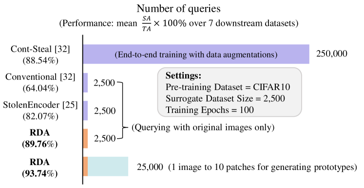
Figure 3: Performance comparisons between four stealing methods against SSL. The presented results are the mean values achieved by each method over seven different downstream classification tasks, with their corresponding query costs. Our proposed RDA can achieve SOTA results with the least query cost.

Extensive experiments show that RDA acquires a favorable trade-off between the query cost (a.k.a, the money cost) and attack efficacy. As depicted in Figure 3, when the target encoder is pre-trained on CIFAR10, RDA averagely outperforms the state-of-the-art (SOTA), i.e., Cont-Steal [19], by 1.22% on the stealing efficacy over seven different downstream datasets, with a competitive smaller query cost, i.e., only 1% of Cont-Steal. Further, this performance gap can be widened to 5.20% with 10% query cost of Cont-Steal. In particular, RDA is demonstrated to be robust against multiple prevalent defenses [8, 31, 14].

In conclusion, our contributions are three folds:

• We comprehensively investigate two critical inadequacies of existing stealing methods against SSL, i.e., suboptimal efficacy and high query costs, and analyze the causes.

• We develop a novel approach to train surrogate encoders, namely RDA, with sample-wise prototype guidance and a multi-relational extraction loss.

• Extensive experiments are conducted to verify the effectiveness and robustness of RDA.

Related Work

Prototype Learning. A prototype refers to the mean of embeddings belonging to all images of an identical class, which serves as a proxy of the class [22]. With each class having a prototype, the model is trained to match its output with the corresponding prototype when inputting a sample of a certain class. Prototype learning has proven beneficial for various learning scenarios, e.g., federated learning [25, 26, 27] and few-shot learning [23, 24, 28]. In this paper, the optimization objective (i.e., the mean of embeddings belonging to an identical sample’s multiple augmentations) we generate for each training sample is conceptually similar to prototypes, and thus we name it a sample-wise prototype.

Model Stealing Attacks against SSL. Dziedzic et al. [17] pointed out that the higher dimension of embeddings (e.g., 2,048 of ResNet50 [16]) leaks more information than labels (e.g., 10 of CIFAR10), making SSL more easily stolen. The primary objective of a stealing attack is to train a surrogate encoder to achieve high accuracy on downstream tasks or recreate a high-fidelity copy that can be used to mount further attacks such as adversarial examples [13] and membership inference attacks [11].

Defense against Model Stealing Attacks. Existing defenses against model stealing attacks can be categorized based on when they are applied [17]. Perturbation-based defenses, e.g., adding noise [8], top-k [8] and truncating outputs [31], are applied before a stealing attack happens, aiming to limit the information leakage. On the other hand, watermarking defenses embed watermarks or unique identifiers into the target model and use them to detect whether it is stolen after a stealing attack happens [32].

Methodology

Threat Model

Given a target encoder $E_{T}$, the attacker aims to train a surrogate encoder $E_{S}$ at the lowest possible cost, which can perform competitively on downstream tasks with $E_{T}$. To achieve this goal, the attacker queries $E_{T}$ for embeddings of an unlabeled surrogated dataset $D_{S}=\{\boldsymbol{x}_{1},\boldsymbol{x}_{2},\dots,\boldsymbol{x}_{N}\}$ consisting of $N$ images, and guide $E_{S}$ to mimic the output of $E_{T}$ for each sample in $D_{S}$. Specifically, we consider a black-box setting, where the attacker has direct access only to the outputs of $E_{T}$ while remaining unaware of its architecture and training configurations, including pre-training datasets, loss functions, data augmentations schemes, etc.

Sample-Wise Prototypes

Recalling the discussion in Section 1, we expect to refine the target encoder’s representations to find a less biased optimization objective for each sample in $D_{S}$. Enlightened by prototype learning [22] and Extreme-Multi-Patch-SSL (EMP-SSL) [6], which establish a prototype/benchmark for each class/sample, we propose a sample-wise prototype generation method for this purpose. In detail, the process of prototype generation can be divided into three steps as follows: ❶ Cropping and augmenting each image $\boldsymbol{x}_{i}\in D_{S}$ into $n$ augmentation patches denoted as $\{\boldsymbol{x}^{\prime}_{i,t,c}\}_{c=1}^{n}=\{\boldsymbol{x}^{\prime}_{i,t,1},\dots,\boldsymbol{x}^{\prime}_{i,t,n}\}$; ❷ Querying $E_{T}$ with each augmentation patch in $\{\boldsymbol{x}^{\prime}_{i,t,c}\}_{c=1}^{n}$, resulting in a set of embeddings denoted as $\{E_{T}(\boldsymbol{x}_{i,t,c})\}_{c=1}^{n}=\{E_{T}(\boldsymbol{x}^{\prime}_{i,t,1}),\dots,E_{T}(\boldsymbol{x}^{\prime}_{i,t,n})\}$; ❸ Calculating the mean of $\{E_{T}(\boldsymbol{x}_{i,t,c})\}_{c=1}^{n}$ as the prototype $p_{\boldsymbol{x}_{i}}$ for $\boldsymbol{x}_{i}$ as follows:

$$p_{\boldsymbol{x}_{i}}=\frac{1}{n}\sum_{c=1}^{n}E_{T}(\boldsymbol{x}^{\prime}_{i,t,c}),\quad\boldsymbol{x}_{i}\in D_{s}.$$ (1)

Each generated prototype $p_{\boldsymbol{x}_{i}},i=1,2,\dots,N$, will be stored in a memory bank. These sample-wise prototypes can provide a stable optimization objective for each sample throughout the training process. Consequently, the attacker can accomplish the training in a query-free manner. Notably, setting $n$ to a value that is far less than the training epochs, e.g., 10 v.s. 100, is sufficient to yield a favorable performance. The prototype generation process is illustrated in step ① of Figure 4. Moreover, Supplementary A.2 explains how we build the memory bank in practice.

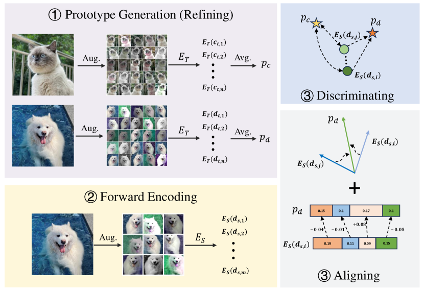
Figure 4: Pipeline of RDA. Prototype generation: augment one sample into $n$ patches and use them to query the target encoder ($E_{T}$). The mean of the $n$ patches’s embeddings is defined as a prototype for this sample. Forward encoding: crop one image into $m$ patches and feed them to the surrogate encoder ($E_{S}$) for their embeddings. Optimization: align embeddings from the surrogate encoder to their matched prototypes in both angle and amplitude while pushing away those belonging to different samples.

Multi-Relational Extraction Loss

As step ② of Figure 4 shows, during training $E_{S}$, we also perform cropping and augmentation on each image $\boldsymbol{x}_{i}\in D_{S}$ to create $m$ patches, forming an augmentation patch set denoted as $\{\boldsymbol{x}^{\prime}_{i,s,q}\}_{q=1}^{m}=\{\boldsymbol{x}^{\prime}_{i,s,1},\dots,\boldsymbol{x}^{\prime}_{i,s,m}\}$. The $m$ does not necessarily need to be set equal to $n$. Next, we feed each augmentation patch from $\{\boldsymbol{x}^{\prime}_{i,s,q}\}_{q=1}^{m}$ to $E_{S}$, obtaining a set of embeddings denoted as $\{E_{S}(\boldsymbol{x}^{\prime}_{i,s,q})\}_{q=1}^{m}=\{E_{S}(\boldsymbol{x}^{\prime}_{i,s,1}),\dots,E_{S}(\boldsymbol{x}^{\prime}_{i,s,m})\}$. To optimize $E_{S}$, we develop a multi-relational extraction loss composed of two parts, i.e., the discriminating loss and the aligning loss.

Discriminating Loss. The discriminating loss is responsible for training $E_{S}$ to distinguish between different samples, as depicted in step ③ (the blue block) of Figure 4. For this goal, it pushes each embedding in $\{E_{S}(\boldsymbol{x}^{\prime}_{i,s,q})\}_{q=1}^{m}$ away from mismatched prototypes $p_{\boldsymbol{x}_{j}},i\neq j$ (denoted as negative pairs). In this regard, contrastive learning [1, 38, 2, 4] offers a solution, as it can pull embeddings of positive pairs close while pushing embeddings of negative pairs apart. Furthermore, since more negative pairs can help improve the performance of contrastive learning [1], we refer to the loss designed by Sha et al. [19] to propose our discriminating loss $\mathcal{L}_{D}$. In particular, $\mathcal{L}_{D}$ considers both mismatched prototype-embedding pairs from different samples as well as embeddings from $E_{S}$ for different samples as negative pairs. Formally, $\mathcal{L}_{D}$ can be expressed as follows:

$$\mathcal{L}_{pos}(\boldsymbol{x}_{i})=\frac{1}{m}\sum_{q=1}^{m}\exp{(sim(E_{S}(\boldsymbol{x}^{\prime}_{i,s,q}),p_{\boldsymbol{x}_{i}})/\tau)},$$ (2)

$$\mathcal{L}_{D}=-\frac{1}{N}\sum_{i=1}^{N}\log{\frac{\mathcal{L}_{pos}(\boldsymbol{x}_{i})}{\mathcal{L}_{neg}(\boldsymbol{x}_{i})}},$$ (4)

where $sim(u,v)$ represents the cosine similarity between $u$ and $v$, and $\tau$ is a temperature parameter.

Aligning Loss. While $\mathcal{L}_{D}$ can separate different samples effectively, it does not fully leverage the potential of prototypes. To further enhance the attack efficacy, we propose to align embeddings from $E_{S}$ more thoroughly with their matched prototypes from the high-performance $E_{T}$, i.e., in terms of both amplitude and angle, as step ③ (the gray block) of Figure 4 shows. To measure the amplitude and angle deviations between two embeddings, we employ the mean square error (MSE) and cosine similarity to quantify them as follows:

$$\mathcal{L}^{\prime}_{amp}(\boldsymbol{x}_{i})=\frac{1}{m}\sum_{q=1}^{m}\|E_{S}(\boldsymbol{x}^{\prime}_{i,s,q})-p_{\boldsymbol{x}_{i}}\|^{2},$$ (5)

$$\mathcal{L}^{\prime}_{ang}(\boldsymbol{x}_{i})=\frac{1}{m}\sum_{q=1}^{m}sim(E_{S}(\boldsymbol{x}^{\prime}_{i,s,q}),p_{\boldsymbol{x}_{i}}).$$ (6)

Notice that we will normalize the value of $\mathcal{L}^{\prime}_{ang}$ to $\left[0,1\right]$. However, there is an issue concerning the equal penalty given by $\mathcal{L}^{\prime}_{amp}$ and $\mathcal{L}^{\prime}_{ang}$ to every deviation increase. For instance, when the MSE increases from 0.8 to 0.9 or from 0.3 to 0.4, both penalties given by $\mathcal{L}^{\prime}_{amp}$ are 0.1, which we deem imprudent. On the contrary, we should have a more rigorous penalty for the increase in MSE from 0.3 to 0.4, as a smaller MSE is more desirable. Likewise, the same penalizing regime should be applied on $1/\mathcal{L}^{\prime}_{ang}$ for the same reason. To this end, we adopt a logarithmic function to redefine the ultimate formulations of $\mathcal{L}_{amp}$ and $\mathcal{L}_{ang}$ as follows:

$$\mathcal{L}_{amp}(\boldsymbol{x}_{i})=\log\mathcal{L}^{\prime}_{amp}(\boldsymbol{x}_{i}),$$ (7)

$$\mathcal{L}_{ang}(\boldsymbol{x}_{i})=\log(1/\mathcal{L}^{\prime}_{ang}(\boldsymbol{x}_{i}))=-\log\mathcal{L}^{\prime}_{ang}(\boldsymbol{x}_{i}).$$ (8)

We posit the amplitude and angle deviations hold equal importance, and formulate the aligning loss as follows:

Lastly, we can express the loss function for stealing pre-trained encoders as follows

$$\mathcal{L}=\lambda_{1}\cdot\mathcal{L}_{D}+\lambda_{2}\cdot\mathcal{L}_{A},$$ (10)

where $\lambda_{1}$ and $\lambda_{2}$ are preset coefficients to adjust the weight of each part in $\mathcal{L}$. To show the superiority of our design, we have conducted ablation studies in Section 4.4 and explored several alternative designs in Supplementary A.3.

In addition, we have summarized the detailed steps of RDA in Algorithm 1 of Supplementary A.2.

Experiments

Experimental Setup

Target Encoder Settings. We use SimCLR [1] to pre-train two ResNet18 encoders on CIFAR10 [40] and STL10 [44], respectively, as two medium-scale target encoders. Furthermore, we consider two real-world large-scale ResNet50 encoders as the target encoders, i.e., the ImageNet encoder pre-trained by Google [1], and the CLIP encoder pre-trained by OpenAI [5]. Besides the ResNet family, RDA also has been demonstrated effective upon other backbones, i.e., VGG19_bn [41], DenseNet121 [42], and MobileNetV2 [43], in Supplementary A.4.

Attack Settings. Regarding the surrogate dataset, we sample it from Tiny ImageNet [49]. Specifically, we randomly sample 2,500 images and resize them to $32\times 32$ for stealing encoders pre-trained on CIFAR10 and STL10. When stealing the ImageNet encoder and CLIP, the number is 40,000 and 60,000, respectively, with each image resized to $224\times 224$. Regarding the surrogate encoder architecture, we adopt a ResNet18 across our experiments. During the attack, we set $n$ in Eq. 1 as 10, $m$ in Eq. 2, 3, 5, and 6 as 5, $\tau$ in Eq. 2 and 3 as 0.07, and both $\lambda_{1}$ and $\lambda_{2}$ in Eq. 10 as 1 except otherwise mentioned. Moreover, the batch size is set as 100, and an Adam optimizer [34] with a learning rate of 0.001 is used to train the surrogate encoder.

Evaluation Settings. We train each surrogate encoder for 100 epochs and test its KNN accuracy [10] on CIFAR10 after each epoch. The best trained, as well as the target encoder, will be used to train downstream classifiers for the linear probing evaluation. Specifically, we totally consider seven downstream datasets, namely MNIST [21], CIFAR10 [40], STL10 [44], GTSRB [45], CIFAR100 [47], SVHN [48], and F-MNIST [46]. Each downstream classifier will be trained for 100 epochs with an Adam optimizer and a learning rate of 0.0001. As done in [18], we use Target Accuracy (TA) to evaluate target encoders, Steal Accuracy (SA) to evaluate surrogate encoders, and $\frac{\text{SA}}{\text{TA}}\times 100\%$ to evaluate the efficacy of the stealing attack.

Effectiveness of RDA

Stealing Medium-Scale Encoders

Table 1 shows the results achieved by RDA upon two medium-scale target encoders pre-trained on CIFAR10 and STL10, respectively. As the results show, using a surrogate dataset of 5% the size of CIFAR10 (2,500 / 50,000) and 2.4% the size of STL10 (2,500 / 105,000), RDA can steal nearly $100\%$ of the functionality of both target encoders, except for the GTSRB scenario when stealing the encoder pre-trained on STL10. Nonetheless, even in this exceptional case, the obtained $\frac{\text{SA}}{\text{TA}}\times 100\%$ is approximately 90%, which exemplifies the remarkable effectiveness of RDA. Furthermore, we observe that the surrogate encoder trained through RDA even outperforms the target encoder on multiple datasets. Our interpretation of this is that the target encoder fits the pre-training dataset more strongly compared to the surrogate encoder trained using RDA, thus exhibiting inferior performance on some out-of-distribution datasets.

Table 1: Results of RDA against two medium-scale encoders.

Pre-training Dataset	Downstream Dataset	TA	SA	$\frac{\text{SA}}{\text{TA}}\times 100\%$
CIFAR10	MNIST	97.27	96.62	99.33
	F-MNIST	88.58	89.32	100.84
	GTSRB	61.76	62.75	101.60
	SVHN	73.78	73.74	99.95
STL10	MNIST	96.84	96.31	99.45
	F-MNIST	90.08	87.91	97.59
	GTSRB	64.45	57.70	89.53
	SVHN	61.85	70.67	114.26

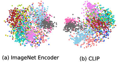
Figure 5: t-SNE of embeddings of 2,000 images randomly sampled from CIFAR10 generated by the ImageNet encoder and CLIP.

Table 2: Results of RDA against the ImageNet Encoder and CLIP.

Target Encoder	Downstream Dataset	TA	SA	$\frac{\text{SA}}{\text{TA}}\times 100\%$
ImageNet Encoder	MNIST	97.38	95.89	98.47
	F-MNIST	91.67	90.83	99.08
	GTSRB	63.14	59.62	94.43
	SVHN	73.20	69.21	94.55
CLIP	MNIST	97.90	93.96	95.98
	F-MNIST	89.92	87.43	97.23
	GTSRB	68.61	55.84	81.39
	SVHN	69.53	57.58	82.81

Table 3: Computation resources required by pre-training the two targeted real-world encoders from scratch and RDA to steal them.

Target Encoder	Pre-training			RDA
	Hardware	Time (hrs)		Hardware	Time (hrs)
ImageNet Encoder	TPU v3	192		RTX A5000	10.8
CLIP	V100 GPU	255,744			16.2

Table 4: The comparison between RDA and three baselines to steal the encoder pre-trained on CIFAR10 under the same surrogate dataset size. We report the $\frac{\text{SA}}{\text{TA}}\times 100\%$ achieved by each method and its query cost. The Optimal and suboptimal results are highlighted.

Method	CIFAR10	CIFAR100	MNIST	GTSRB	SVHN	STL10	F-MNIST	Queries
Conventional [19]	63.36	45.40	96.16	20.34	68.26	60.25	94.52	2,500
StolenEncoder [18]	79.03	68.78	98.76	63.70	92.01	76.29	95.91	2,500
Cont-Steal [19]	80.43	73.94	98.03	95.55	96.39	80.08	95.39	250,000
RDA	83.84	77.49	98.97	94.27	96.79	82.25	94.69	2,500
	85.85	83.08	99.33	101.60	99.95	85.56	100.84	25,000

Stealing Real-World Large-Scale Encoders

We further evaluate RDA on two real-world pre-trained encoders, i.e., the ImageNet encoder and CLIP. We aim to demonstrate the effectiveness of RDA upon such large-scale encoders trained with a massive amount of data. Specifically, the ImageNet encoder is pre-trained on the ImageNet dataset, which has 1.3 million images. The CLIP encoder is pre-trained on a web-scale dataset that consists of 400 million image-text pairs. During the attack, we set the patch number for training as 1 (i.e., $m$ in Eq. 2, 3, 5, and 6) to save time. Other parameters follow the default setting except the $\lambda_{1}$ and $\lambda_{2}$ when stealing CLIP, in which we set $\lambda_{1}$ and $\lambda_{2}$ to 1 and 20, respectively. To interpret the reason for this adjustment, we randomly sample 200 images from each class in the testing set of CIFAR10 and visualize the output embeddings from the ImageNet encoder and CLIP using t-SNE [50]. Figure 5 shows that embeddings from the ImageNet encoder are more uniformly distributed compared to those from CLIP. This is because CLIP is a multimodal encoder, which is pre-trained by conducting contrastive learning between image-text pairs. Therefore, the text also shares part of the embedding space and is mutually exclusive with mismatched images. Although $\mathcal{L}_{D}$ can push embeddings of different samples apart, a significant weight of it will make all embeddings more uniformly distributed, i.e., not align with CLIP. Therefore, we set a small weight to $\mathcal{L}_{D}$ when stealing CLIP. This adjustment is practical since the attacker has access to the outputs of the target encoder, and thus can observe its embedding space to adjust its attack settings. Table 2 shows that using a surrogate dataset of only 3.07% the size of ImageNet (40K / 1.3M) and 0.015% the size of the training data of CLIP (60K / 400M), RDA can achieve comparable performances with the two encoders across various downstream tasks. The results also reveal that even under the architecture of the surrogate and target encoders being distinct (ResNet18 v.s. ResNet50), RDA still exhibits high effectiveness. Moreover, Table 3 shows that RDA requires much fewer computation resources to steal the two encoders than pre-training them from scratch, owing to the small surrogate dataset and lightweight network architecture.

Comparision with Existing Methods

We consider the conventional method (CVPR 2023) [19], StolenEncoder (CCS 2022) [18], and Cont-Steal (CVPR 2023) [19] as our baselines. A more detailed explanation of them can be found in Supplementary A.1. Specifically, we compare RDA with them to steal the encoder pre-trained on CIFAR10 under three different scenarios as follows:

Table 5: The comparison between RDA and StolenEncoder under the same query cost. Optimal results are highlighted.

Queries	Method	setting	SA
2500	StolenEnoder	2,500 images	71.98
	RDA	500 images$\times$5 patches	65.38
		625 images$\times$4 patches	67.07
		1,250 images$\times$2 patches	71.44
		2,500 images$\times$ 1 patch	76.36
25,000	StolenEnoder	25,000 images	76.23
	RDA	2,500 images$\times$10 patches	78.50

Under the Same Surrogate Dataset Size

In this subsection, we fix the surrogate dataset size to 2,500 and make it identical across all methods. As Table 4 shows, RDA outperforms baselines by a significant margin across all seven downstream datasets with a moderate query cost. We also evaluate RDA under a setting that has the same query cost as the conventional method and StolenEncoder (i.e., 2,500 queries), for which we query with each sample once in its origin version. The results show that RDA still surpasses baselines over five out of seven datasets with the least query cost. In addition, the comparison between the results achieved by RDA with 25,000 and 2,500 queries reveals that more patches for generating prototypes will enhance the attack. The embedding space of the surrogate encoder trained by each method is visualized in Figure 10 of Supplementary A.4, which shows that our RDA can train surrogate encoders to discriminate different samples better. Besides, We have summarized the mean value achieved by each method over the seven downstream datasets in Figure 3 to show the superiority of RDA.

Under the Same Query Cost

To demonstrate the superiority of RDA against baselines under an identical query cost, we consider two fixed values, i.e., 2,500 and 25,000. We take StolenEncoder as the rival since it is the best baseline with the least query cost. We note that Cont-Steal is beyond our consideration because the data volume for it would be too small under such a setting, which is only 25 images for 2,500 queries and 250 images for 25,000 queries. $N$ images $\times$ $n$ patches in the table indicates that we use $N$ images as the surrogate dataset and crop each image into $n$ patches to generate prototypes. Therefore, the query cost of RDA is $N\times n$. As shown in Table 5, under the same query cost of 2,500, RDA can achieve comparable results with StolenEncoder with half the size of its surrogate dataset. With the same 2,500 images, RDA outperforms StolenEncoder by a significant margin, showcasing its superiority. Moreover, under a query cost of 25,000, RDA outperforms StolenEncoder by 2.14% with only 10% the size of its surrogate dataset. Besides, comparisons between different configurations of RDA under queries of 2,500 indicate that the training data volume has a dominant impact on the performance.

Under the Same Time Cost

Since each sample is also cropped and augmented into multiple patches for training (i.e., needing to forward encode each sample multiple times), RDA takes the longest time for training. Table 10 in Supplementary A.4 contains the detailed time cost of each method. To make a fair comparison, we prolong the training for another 200 epochs for baseline methods, i.e., 300 epochs in total, which is sufficient to lead their performances to saturate. The trained surrogate encoders are then evaluated on CIFAR10 as the downstream dataset. Figure 6 reveals that even though baseline methods take longer time to train, RDA still outperforms them with the least query cost, and the performance gap can be further widened by a moderate query cost.

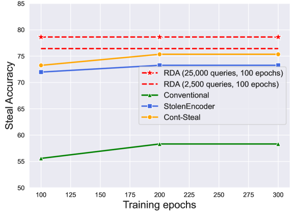
Figure 6: The comparison between RDA and three baselines under the same time cost. The training epochs of RDA are fixed to 100 while those of baseline methods are prolonged to 300.

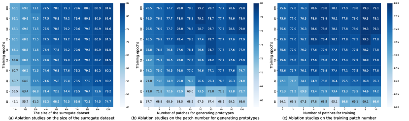
Figure 7: Heat map of the SAs achieved by stealing attacks. This figure shows the performance of 100 combinations of different training epochs and (a) the surrogate dataset size, (b) the patch number for generating prototypes, and (c) the patch number for training.

Ablation Studies

In this subsection, we conduct ablation studies to investigate the impact of the surrogate dataset size, the patch number for generating prototypes (i.e., $n$ in Eq. 1), the patch number for training (i.e., $m$ in Eq. 2, 3, 5, and 6), and loss functions. All the experiments are conducted to steal the encoder pre-trained on CIFAR10. Regarding evaluations, the trained surrogate encoders are evaluated on CIFAR10 in the former three ablations studies. While investigating the impact of loss functions, we consider four different downstream datasets, i.e., F-MNIST, GTSRB, SVHN, and a challenging CIFAR100. Other configurations are fixed to the default setting and we report the achieved SA as results.

Surrogate Dataset Size

Recall our default setting where we randomly sample 2,500 images from Tiny ImageNet to construct the surrogate dataset, which is 5% the size of CIFAR-10. We vary the ratio from 1% to 10% to investigate its impact. Figure 7 (a) shows that a larger surrogate dataset will accelerate the training and improve the attack performance.

Patch Number for Generating Prototypes

We vary the patch number for generating prototypes from 1 to 100 to investigate its impact. Figure 7 (b) shows that there is a tendency for more patches for generating prototypes will improve the attack performance and accelerate the convergence. However, when the patch number reaches 10, more patches do not further improve the attack performance due to the limited surrogate dataset size.

Table 6: Ablation studies on loss functions. The results are SAs on different downstream datasets, with highlighting the optimal.

Loss Type	CIFAR100	F-MNIST	GTSRB	SVHN
Target Encoder	53.29	88.58	61.76	73.78
MSE	31.00	86.12	32.79	62.97
Cosine Similarity	43.81	88.76	55.53	75.94
KL Divergence	40.98	87.82	57.04	69.38
InfoNCE	39.24	87.86	58.82	68.88
$\mathcal{L}_{D}$	43.16	89.27	65.77	71.15
$\mathcal{L}_{A}$	43.79	89.24	55.96	76.70
$\mathcal{L}_{A}+\mathcal{L}_{D}$	44.27	89.32	62.75	73.74

Patch Number for Training

We vary the patch number for training from 1 to 10 to investigate its impact. Figure 7 (c) reveals a tendency for more patches for training will accelerate the training and achieve better results. However, more patches also indicate longer training time and more computation resources.

Loss Functions.

To demonstrate the superiority of the design of our loss function and the necessity of each part, we conduct ablation studies as shown in Table 6. Table 6 shows that $\mathcal{L}_{D}$ achieves the best result on GTSRB, while $\mathcal{L}_{A}$ achieves the best result on SVHN. We hypothesize that $\mathcal{L}_{A}$ attains optimal outcomes on SVHN due to the pronounced resemblance between SVHN and the surrogate dataset. It appears that $\mathcal{L}_{A}$ inclines towards inducing the surrogate encoder to overfit the surrogate data, thereby elucidating its suboptimal performance on GTSRB, a dataset characterized by less similarity with the surrogate dataset. On the contrary, $\mathcal{L}_{D}$ makes the surrogate encoder fit less to the surrogate dataset and has the best result on GTSRB. To further investigate the effect of each part in our loss, we have conducted an ablation experiment in Supplementary A.4 about the weight of each part in our loss. The results show that as the weight of $\mathcal{L}_{A}$ increases, the surrogate encoder will perform better on SVHN while worse on GTSRB. We refer to Supplementary A.4 for a more detailed analysis. Combining $\mathcal{L}_{D}$ and $\mathcal{L}_{A}$, our loss is the most robust one, which achieves the best results on F-MNIST and the most challenging CIFAR100, while also achieving decent results on GTSRB and SVHN.

Robustness to Defenses

In this section, we evaluate the robustness of RDA against three perturbation-based defenses that aim to limit information leakage and one watermarking defense that aims to detect whether a suspected encoder is stolen. The pre-training and downstream datasets both are set to CIFAR10.

Perturbation-Based Defense

We evaluate three common practices of this type of defense, i.e., adding noise [8], top-k [8] and rounding [31].

$\bullet$ Adding noise: Adding noise means that the defender will introduce noise to the original output embeddings of the target encoder. Specifically, we set the mean of the noise to 0 and vary the standard deviations to control the noise level.

$\bullet$ Top-k: Top-k means that the defender will only output the first $k$ largest number of each embedding from the target encoder and set the rest as 0. We vary the value of $k$ to simulate different perturbation levels.

$\bullet$ Rounding: Rounding means that each value in the embedding will be truncated for a specific precision. We vary the precision to simulate different perturbation levels.

The results of the three perturbation-based defense methods are summarized in (a), (b), and (c) of Figure 8, respectively. We can observe in Figure 8 (a) that while adding noise can mitigate the model stealing attack, it decreases the utility of the target encoder more significantly. Moreover, Figure 8 (b) shows that though Top-k can decrease the efficacy of RDA as the defender lowers the value of k, it also severely deteriorates the target encoder’s performance. On the other hand, Figure 8 (c) reveals that rounding has a minimal effect on the performance of both the target encoder and attack. Our experimental results demonstrate the robustness of RDA against perturbation-based defenses.

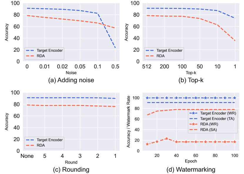
Figure 8: The performance of different defense methods. Pre-training and downstream datasets both are CIFAR10.

Watermarking Defense

As shown by Adi et al. [12], backdoors can be used as watermarks to claim the ownership of a model. In this sense, we follow [19] and leverage BadEncoder [14] to embed a backdoor into the target encoder as the watermark. Ideally, if the watermarked encoder is stolen, the surrogate encoder trained via stealing should also be triggered by the defender-specified trigger to exhibit certain behaviors, and thus the ownership can be claimed. Fortunately, Figure 8 (d) shows that RDA can steal the functionality of the target encoder while unlearning the watermark. More specifically, the watermark rate (WR) of the target encoder is 99.87% but only 17.04% for the surrogate encoder when the training converges. This observation indicates that the watermark embedded in the target encoder cannot be preserved by RDA.

Conclusion

In this paper, we have proposed a novel model stealing method against SSL named RDA, which stands for refine, discriminate, and align. Compared with previous methods [18, 19], RDA establishes a less biased optimization objective for each training sample and strives to extract more abundant functionality of the target encoder. This empowers RDA to exhibit tremendous effectiveness and robustness across diverse datasets and settings.

Limitation and Future Work. The query cost of RDA is not yet optimal and can be further reduced by techniques like clustering to establish an identical prototype for multiple similar images. We leave this for future work.

Appendix A Supplementary Material

Elaborations on Existing Methods

In this section, we will elaborate on the three baselines considered in this paper, namely, the conventional method [19], StolenEnoder [18], and Cont-Steal [19].

$\bullet$ Conventional method: Given a surrogate dataset $D_{S}=\{\boldsymbol{x}_{1},\boldsymbol{x}_{2},\dots,\boldsymbol{x}_{N}\}$, the conventional method first queries the target encoder $E_{T}$ once with each sample $\boldsymbol{x}_{i}\in D_{S}$. The output embedding $E_{T}(\boldsymbol{x}_{i}),i=1,2,\dots,N,$ will be stored in a memory bank to serve as a “ground truth” for the sample across the whole training. Next, to train the surrogate encoder $E_{S}$, it feeds each sample $\boldsymbol{x}_{i}\in D_{S}$ to $E_{S}$ and pulls the output embedding $E_{S}(\boldsymbol{x}_{i})$ close to its corresponding optimization objective, i.e., $E_{T}(\boldsymbol{x}_{i})$.

$\bullet$ StolenEncoder: Similar to the conventional method, StolenEncoder first queries the target encoder $E_{T}$ once with each sample $\boldsymbol{x}_{i}\in D_{S}$ and stores the output embedding $E_{T}(\boldsymbol{x}_{i}),i=1,2,\dots,N,$ in a memory bank. Next, it not only feeds each sample $\boldsymbol{x}_{i}\in D_{S}$ but also an augmentation $\boldsymbol{x}^{\prime}_{i}$ of it to the surrogate encoder $E_{S}$. The output embeddings $E_{S}(\boldsymbol{x}_{i})$ and $E_{S}(\boldsymbol{x}^{\prime}_{i})$ will be pulled close to $E_{T}(\boldsymbol{x}_{i})$ simultaneously for optimizing the surrogate encoder $E_{S}$.

$\bullet$ Cont-Steal: In particular, Cont-Steal adopts an end-to-end training strategy to train the surrogate encoder $E_{S}$. In each epoch, Cont-Steal first augments each image $\boldsymbol{x}_{i}\in D_{S}$ into two perspectives, denoted as $\boldsymbol{x}^{\prime}_{i,t}$ and $\boldsymbol{x}^{\prime}_{i,s}$, respectively. Next, $\boldsymbol{x}^{\prime}_{i,t}$ is used to query the target encoder $E_{T}$, while $\boldsymbol{x}^{\prime}_{i,s}$ is fed to the surrogate encoder $E_{S}$. The surrogate encoder then is optimized via contrastive learning that pulls $E_{T}(\boldsymbol{x}^{\prime}_{i,t})$ and $E_{S}(\boldsymbol{x}^{\prime}_{i,s})$ close while pushing $E_{S}(\boldsymbol{x}^{\prime}_{k,s}),k\neq i,$ and $E_{T}(\boldsymbol{x}^{\prime}_{i,t})$ apart. Moreover, to enhance contrastive learning, Cont-Steal also includes $E_{S}(\boldsymbol{x}^{\prime}_{i,s})$ and $E_{S}(\boldsymbol{x}^{\prime}_{k,s}),i\neq k,$ as negative pairs to train $E_{S}$.

Table 7: Query cost analysis of three baseline methods.

Method	Surrogate Dataset Size	Training Epoch	Query Cost
Conventioanl [19]	$N$	$L$	$N$
StolenEncoder [18]	$N$	$L$	$N$
Cont-Steal [19]	$N$	$L$	$N\times L$

Query Cost Analysis. Assuming the attacker has a surrogate dataset $D_{S}=\{\boldsymbol{x}_{1},\boldsymbol{x}_{2},\dots,\boldsymbol{x}_{N}\}$ consisting of $N$ images. To train a surrogate encoder, the attacker will use $D_{S}$ to query the target encoder and optimize the surrogate encoder to mimic its outputs. Regarding the conventional method and StolenEncoder, each image $\boldsymbol{x}_{i}\in D_{s}$ will be used to query only once. Therefore, the query cost of them is $N$, and nothing about the number of training epochs. As for Cont-Steal, each image in $D_{S}$ will be augmented into two perspectives and one is used to query the target encoder in each epoch. Therefore, assuming the training will last for $L$ epochs, the query cost of Cont-Steal is $N\times L$. Although Cont-Steal achieves superior results, its query cost is formidable since the training typically requires over 100 epochs to converge. We have the query cost of each method summarized in Table 7.

input : Surrogate dataset $D_{S}$, target encoder $E_{T}$, surrogate encoder $E_{S}$, patch number $n$ for generating prototypes and $m$ for training.

output : A high-performance surrogate encoder $E_{S}$

1

2Load $E_{T}$ and initialize $E_{S}$.

3

4Prototype generation:

5

6for each image $\boldsymbol{x}_{i}\in D_{S}$ do

7       augment $\boldsymbol{x}_{i}$ into into multiple patches $\{\boldsymbol{x}^{\prime}_{i,t,c}\}_{c=1}^{n}=\{\boldsymbol{x}^{\prime}_{i,t,1},\dots,\boldsymbol{x}^{\prime}_{i,t,n}\}$;

8       query $E_{T}$ with $\{\boldsymbol{x}^{\prime}_{i,t,c}\}_{c=1}^{n}$ and obtain $\{E_{T}(\boldsymbol{x}^{\prime}_{i,t,c})\}_{c=1}^{n}=\{E_{T}(\boldsymbol{x}^{\prime}_{i,t,1}),\dots,E_{T}(\boldsymbol{x}^{\prime}_{i,t,n})\}$;

9       calculate the sample-wise prototype for $\boldsymbol{x}_{i}$ as follows: $p_{\boldsymbol{x}_{i}}=\frac{1}{n}\sum_{c=1}^{n}E_{T}(\boldsymbol{\boldsymbol{x}}^{\prime}_{i,t,c})$;

10 end for

11

12Training:

13 for each epoch do

14       for each image $\boldsymbol{x}_{i}\in D_{S}$ do

15             augment $\boldsymbol{x}_{i}$ into multiple patches $\{\boldsymbol{x}^{\prime}_{i,s,q}\}_{q=1}^{m}=\{\boldsymbol{x}^{\prime}_{i,s,1},\dots,\boldsymbol{x}^{\prime}_{i,s,m}\}$;

16             feed $\{\boldsymbol{x}^{\prime}_{i,s,q}\}$ into $E_{S}$ and obtain $\{E_{S}(\boldsymbol{x}^{\prime}_{i,s,q})\}_{q=1}^{m}=\{E_{S}(\boldsymbol{x}^{\prime}_{i,s,1}),\dots,E_{S}(\boldsymbol{x}^{\prime}_{i,s,m})\}$;

17            

18            for each $E_{S}(\boldsymbol{x}^{\prime}_{i,s,1})\in\{E_{S}(\boldsymbol{x}^{\prime}_{i,s,q})\}_{q=1}^{m}$ do

19                   optimize $E_{S}$ with $\mathcal{L}=\lambda_{1}\cdot\mathcal{L}_{D}+\lambda_{2}\cdot\mathcal{L}_{A}$ based on Eq. 2-10;

20                  

21             end for

22            

23       end for

24      

25 end for

return: the trained surrogate encoder $E_{S}$

Algorithm 1 Detailed steps of RDA

Details about Our Method

Practical Formulation of the Memory Bank. In practice, we assign a unique label to each image in the attacker’s surrogate dataset as its key in the memory bank. Specifically, we transform $D_{s}=\{\boldsymbol{x}_{1},\boldsymbol{x}_{2},\dots,\boldsymbol{x}_{N}\}$ into a set of image-key pairs, i.e., $D_{s}=\{(\boldsymbol{x}_{1},1),(\boldsymbol{x}_{2},2),\dots,(\boldsymbol{x}_{n},n)\}$. Then we generate a prototype for each image and get a set of key-prototype pairs that can be expressed as $P=\{1:p_{\boldsymbol{x}_{1}},2:p_{\boldsymbol{x}_{2}},\dots,n:p_{\boldsymbol{x}_{n}}\}$. The prototype set $P$ is stored in a memory bank and we do not need to query the target model anymore.

Detailed Steps. We have the detailed steps of RDA summarized in Algorithm 1.

Table 8: Results of different loss designs. The results are SAs on different downstream datasets, with highlighting the optimal.

Loss Type	CIFAR100	F-MNIST	GTSRB	SVHN
$\mathcal{L}$ (current used)	44.27	89.32	62.75	73.74
$\mathcal{L}_{v2}$	41.99	85.45	61.92	72.88
$\mathcal{L}_{v3}$	42.23	88.63	62.46	71.86

Table 9: Ablation studies on the weights of $\mathcal{L}_{amp}$ and $\mathcal{L}_{ang}$. The results are SAs on different downstream datasets, with highlighting the optimal.

$\mathcal{L}_{amp}:\mathcal{L}_{ang}$	CIFAR100	F-MNIST	GTSRB	SVHN
$5:1$	42.90	86.52	61.32	70.57
$2:1$	43.61	86.80	62.55	72.90
$1:1$	44.27	89.32	62.75	73.74
$1:2$	42.70	88.64	60.59	72.05
$1:5$	43.24	89.16	62.04	73.11

Loss Designs

Alternative Loss designs

In this section, we consider two alternative loss designs about $\mathcal{L}_{A}$. For simplicity, we denote them as $\mathcal{L}_{A,v2}$ and $\mathcal{L}_{A,v3}$, respectively.

$\bullet$ $\mathcal{L}_{A,v2}$: To investigate the benefits of penalizing different deviations with different levels, we define $\mathcal{L}_{A,v2}$ as a naive combination of $\mathcal{L}^{\prime}_{amp}$ and $\mathcal{L}^{\prime}_{ang}$ as follows:

$$\mathcal{L}_{A,v2}=\frac{1}{N}\sum_{i=1}^{N}(\mathcal{L}^{\prime}_{amp}(\boldsymbol{x}_{i})-\mathcal{L}^{\prime}_{ang}(\boldsymbol{x}_{i})).$$ (11)

$\bullet$ $\mathcal{L}_{A,v3}$: To investigate the benefits of our current penalizing regime employed by $\mathcal{L}_{A}$, we reverse it here by an “$\exp$”, i.e., penalizing the MSE increase from 0.8 to 0.9 more harshly than that from 0.3 to 0.4, with the same rule employed on the reciprocal of the cosine similarity. Therefore, we formulate the $\mathcal{L}_{A,v3}$ as follows:

$$\mathcal{L}_{A,v3}=\frac{1}{N}\sum_{i=1}^{N}(\exp{(\mathcal{L}^{\prime}_{amp}(\boldsymbol{x}_{i}))}+\exp{(1/\mathcal{L}^{\prime}_{ang}(\boldsymbol{x}_{i}))}).$$ (12)

Finally, we define:

$$\mathcal{L}_{v2}=\mathcal{L}_{D}+\mathcal{L}_{A,v2},$$ (13)

$$\mathcal{L}_{v3}=\mathcal{L}_{D}+\mathcal{L}_{A,v3}.$$ (14)

We use the encoder pre-trained on CIFAR10 as the target encoder and evaluate the trained surrogate encoders on four different downstream datasets, i.e., CIFAR100, F-MNIST, GTSRB, and SVHN. Each experiment is run three times and we report the mean value of the achieved SAs by each loss design in Table 8.

As the results show, both $\mathcal{L}_{v2}$ and $\mathcal{L}_{v3}$ underperform $\mathcal{L}$. On the one hand, $\mathcal{L}$ outperforms $\mathcal{L}_{v2}$ indicating that incorporating our current penalizing regime is beneficial. On the other hand, $\mathcal{L}$ outperforms $\mathcal{L}_{v3}$ indicating that penalizing a deviation from a more favorable value to a worse one more harshly is more favorable upon the opposite penalizing regime.

The Weights of Amplitude and Angle Deviations

Recall our default setting that we assume the amplitude and angle deviations are of equal importance and thus formulate $\mathcal{L}_{A}(\boldsymbol{x}_{i})=\mathcal{L}_{amp}(\boldsymbol{x}_{i})+\mathcal{L}_{ang}(\boldsymbol{x}_{i})$. Here we ablate on five different weight pairs as shown in Table 9 to investigate the importance level of each deviation type. From the results, we can see that setting the weights of $\mathcal{L}_{amp}$ and $\mathcal{L}_{ang}$ to $1:1$ generally achieves the best result.

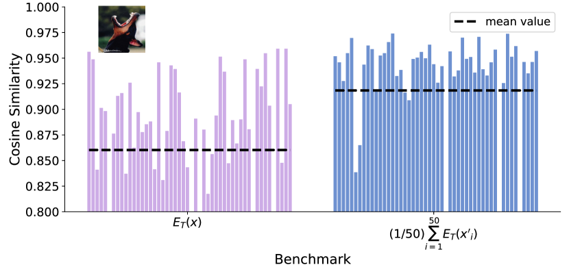
Figure 9: We augment an image $\boldsymbol{x}$ into 50 patches and feed them into an encoder $E_{T}$ that pre-trained on CIFAR10 (KNN Accuracy = 88.31%, tested on CIFAR10). This figure depicts the cosine similarity between each augmentation patch’s embedding and two different benchmarks, i.e., (1) the embedding of the original image and (2) the prototype of the image, with the mean value over the 50 similarities marked in the dashed line. We can see that the prototype is significantly more similar to each patch’s embedding, showcasing it is less biased.

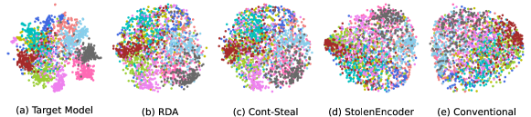
Figure 10: t-SNE of embeddings of 2,000 images randomly sampled from CIFAR10 generated by the target encoder and surrogate encoders trained with different methods.

Supplementary Experiments

Benifit of Using Prototypes. We augment an image $\boldsymbol{x}$ (stamped at the upper left corner of Figure 9) into 50 patches and denote each of them as $\boldsymbol{x}^{\prime}_{i},i=1,\dots,50$. Next, we input each patch as well as the image’s original version into $E_{T}$, an encoder pre-trained on CIFAR10. To show the image’s prototype (i.e., $\frac{1}{50}\sum_{i=1}^{50}E_{T}(\boldsymbol{x}^{\prime}_{i})$) is a less biased optimization objective compared to the embedding of its original version (i.e., $E_{T}(\boldsymbol{x})$), we depict the cosine similarity between each patch’s embedding and the two different benchmarks in Figure 9. We can see that the prototype has significantly higher similarity with each patch’s embedding, showcasing it is less biased.

Visualization of the Embedding Space. To visualize the embedding space of the surrogate encoder trained by each method, we randomly sample 200 images from each class of CIFAR10 (i.e., 2,000 images in total) and feed them to the surrogate encoder. From Figure 10, we can observe that embeddings of different classes from surrogate encoders trained by StolenEncoder and the conventional method overlap with each other and exhibit less structural clarity. In contrast, RDA and Cont-Steal train surrogate encoders that generate more distinguishable embeddings for different classes. This indicates that encoder stealing benefits from contrastive learning.

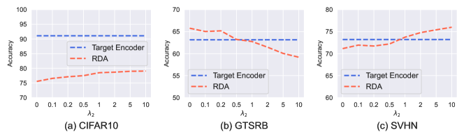
Figure 11: Ablation studies on the weight of each part in the loss, where we fix $\lambda_{1}$ to 1 and vary the value of $\lambda_{2}$ from 0 to 10.

Time Cost. In particular, the total training time comprises two parts, i.e., the time for training the surrogate encoder and the time for testing the trained surrogate encoder after each training epoch to choose the best one. We present the total time cost of each method in Table 10. We can see that the testing time is 13.18 minutes and is identical across all methods over 100 epochs, while the training time of RDA is the longest. This is because RDA augments each image into 5 patches by default to train the surrogate encoder, which means 5 times forward encoding for each image. For a fair comparison, we prolong the training for another 200 epochs for each baseline method and show that our RDA still surpasses them by a large margin.

Table 10: The time cost of each method over the 100 training epochs. Each result consists of two parts, i.e., the time for training the surrogate encoder and the time for testing after each epoch.

Method	Time (min)
Conventional	3.87 $+$ 13.18
StolenEncoder	5.53 $+$ 13.18
Cont-Steal	4.08 $+$ 13.18
RDA	10.65 $+$ 13.18

Effectiveness of RDA on Different Encoder Architectures. To demonstrate the effectiveness of our RDA against pre-trained encoders of various architectures, we further evaluate it on ResNet34, VGG19_bn [41], DenseNet121 [42], and MobileNetV2 [43]. Table 11 shows that RDA can achieve comparable performances with the target encoders of various architectures and even outperforms them on multiple datasets.

Table 11: Results of RDA against target encoders of different architectures. The pre-training dataset is CIFAR10 and the architecture of the surrogate encoder is ResNet18.

Target Encoder Architecture	Downstream Dataset	TA	SA	$\frac{\text{SA}}{\text{TA}}\times 100\%$
ResNet34	MNIST	96.42	96.19	99.76
	F-MNIST	89.51	87.03	97.23
	GTSRB	62.79	54.57	86.91
	SVHN	61.68	70.12	113.68
VGG19_bn	MNIST	90.76	91.57	100.89
	F-MNIST	68.54	74.28	108.37
	GTSRB	13.27	11.25	84.78
	SVHN	26.32	41.30	156.91
DenseNet121	MNIST	95.81	96.15	100.35
	F-MNIST	86.75	88.79	102.35
	GTSRB	54.69	52.05	95.17
	SVHN	49.52	67.19	135.68
MobileNetV2	MNIST	90.56	94.53	104.38
	F-MNIST	77.69	83.38	107.32
	GTSRB	33.88	24.00	70.84
	SVHN	27.54	58.54	212.56

Ablation Studies on the Weight of Each Part in the Loss Function. To investigate the impact of each part in our loss function on the stealing performance, we fix $\lambda_{1}$ in Eq. 10 to 1 and vary the value of $\lambda_{2}$ (i.e., the weight of the aligning loss $\mathcal{L}_{A}$) from 0 to 10. We use the encoder pre-trained on CIFAR10 as the target encoder and evaluate the trained surrogate encoder on three different downstream datasets, i.e., CIFAR10, GTSRB, and SVHN. As we can observe in Figure 11, the surrogate encoders’ performances on CIFAR10 and SVHN positively correlate to the weight of $\mathcal{L}_{A}$, i.e., $\lambda_{2}$. This is because CIFAR10 is the pre-training dataset of the target encoder. As the weight of the aligning loss $\mathcal{L}_{A}$ increases, the outputs of the surrogate and the target encoder become more aligned, and thus the trained surrogate encoder will perform better on CIFAR10. On the other hand, a larger weight for $\mathcal{L}_{A}$ will make the surrogate encoder fit the surrogate dataset more. In this sense, since SVHN is more similar to the surrogate dataset (i.e., Tiny ImageNet), the surrogate encoder naturally performs better on it as the $\lambda_{2}$ increases. On the contrary, as the weight of $\mathcal{L}_{A}$ increases, the surrogate encoder’s performance on GTSRB which shares little similarity with both the pre-training and surrogate datasets becomes worse. Similar phenomenons have been discussed in Section 4.4, where $\mathcal{L}_{D}$ trains the surrogate encoder that achieves the optimal performance on GTSRB. A larger weight for $\mathcal{L}_{A}$ will make the surrogate encoder fit the surrogate dataset more, and thus perform worse on GTSRB.

References

- [1] T. Chen, S. Kornblith, M. Norouzi, and G. Hinton, “A simple framework for contrastive learning of visual representations,” in International conference on machine learning. PMLR, 2020, pp. 1597–1607.
- [2] K. He, H. Fan, Y. Wu, S. Xie, and R. Girshick, “Momentum contrast for unsupervised visual representation learning,” in Proceedings of the IEEE/CVF conference on computer vision and pattern recognition, 2020, pp. 9729–9738.
- [3] J.-B. Grill, F. Strub, F. Altché, C. Tallec, P. Richemond, E. Buchatskaya, C. Doersch, B. Avila Pires, Z. Guo, M. Gheshlaghi Azar et al., “Bootstrap your own latent-a new approach to self-supervised learning,” Advances in neural information processing systems, vol. 33, pp. 21 271–21 284, 2020.
- [4] X. Chen, H. Fan, R. Girshick, and K. He, “Improved baselines with momentum contrastive learning,” arXiv preprint arXiv:2003.04297, 2020.
- [5] A. Radford, J. W. Kim, C. Hallacy, A. Ramesh, G. Goh, S. Agarwal, G. Sastry, A. Askell, P. Mishkin, J. Clark et al., “Learning transferable visual models from natural language supervision,” in International conference on machine learning. PMLR, 2021, pp. 8748–8763.
- [6] S. Tong, Y. Chen, Y. Ma, and Y. Lecun, “Emp-ssl: Towards self-supervised learning in one training epoch,” arXiv preprint arXiv:2304.03977, 2023.
- [7] X. Liu, F. Zhang, Z. Hou, L. Mian, Z. Wang, J. Zhang, and J. Tang, “Self-supervised learning: Generative or contrastive,” IEEE transactions on knowledge and data engineering, vol. 35, no. 1, pp. 857–876, 2021.
- [8] T. Orekondy, B. Schiele, and M. Fritz, “Knockoff nets: Stealing functionality of black-box models,” in Proceedings of the IEEE/CVF conference on computer vision and pattern recognition, 2019, pp. 4954–4963.
- [9] S. Pal, Y. Gupta, A. Shukla, A. Kanade, S. Shevade, and V. Ganapathy, “A framework for the extraction of deep neural networks by leveraging public data,” arXiv preprint arXiv:1905.09165, 2019.
- [10] Z. Wu, Y. Xiong, S. X. Yu, and D. Lin, “Unsupervised feature learning via non-parametric instance discrimination,” in Proceedings of the IEEE conference on computer vision and pattern recognition, 2018, pp. 3733–3742.
- [11] H. Liu, J. Jia, W. Qu, and N. Z. Gong, “Encodermi: Membership inference against pre-trained encoders in contrastive learning,” in Proceedings of the 2021 ACM SIGSAC Conference on Computer and Communications Security, 2021, pp. 2081–2095.
- [12] Y. Adi, C. Baum, M. Cisse, B. Pinkas, and J. Keshet, “Turning your weakness into a strength: Watermarking deep neural networks by backdooring,” in 27th USENIX Security Symposium (USENIX Security 18), 2018, pp. 1615–1631.
- [13] N. Carlini and D. Wagner, “Towards evaluating the robustness of neural networks,” in 2017 ieee symposium on security and privacy (sp). Ieee, 2017, pp. 39–57.
- [14] J. Jia, Y. Liu, and N. Z. Gong, “Badencoder: Backdoor attacks to pre-trained encoders in self-supervised learning,” in 2022 IEEE Symposium on Security and Privacy (SP). IEEE, 2022, pp. 2043–2059.
- [15] T. Brown, B. Mann, N. Ryder, M. Subbiah, J. D. Kaplan, P. Dhariwal, A. Neelakantan, P. Shyam, G. Sastry, A. Askell et al., “Language models are few-shot learners,” Advances in neural information processing systems, vol. 33, pp. 1877–1901, 2020.
- [16] K. He, X. Zhang, S. Ren, and J. Sun, “Deep residual learning for image recognition,” in Proceedings of the IEEE conference on computer vision and pattern recognition, 2016, pp. 770–778.
- [17] A. Dziedzic, N. Dhawan, M. A. Kaleem, J. Guan, and N. Papernot, “On the difficulty of defending self-supervised learning against model extraction,” in International Conference on Machine Learning. PMLR, 2022, pp. 5757–5776.
- [18] Y. Liu, J. Jia, H. Liu, and N. Z. Gong, “Stolenencoder: stealing pre-trained encoders in self-supervised learning,” in Proceedings of the 2022 ACM SIGSAC Conference on Computer and Communications Security, 2022, pp. 2115–2128.
- [19] Z. Sha, X. He, N. Yu, M. Backes, and Y. Zhang, “Can’t steal? cont-steal! contrastive stealing attacks against image encoders,” in Proceedings of the IEEE/CVF Conference on Computer Vision and Pattern Recognition, 2023, pp. 16 373–16 383.
- [20] A. v. d. Oord, Y. Li, and O. Vinyals, “Representation learning with contrastive predictive coding,” arXiv preprint arXiv:1807.03748, 2018.
- [21] Y. LeCun and C. Cortes, “MNIST handwritten digit database,” 2010. [Online]. Available: http://yann.lecun.com/exdb/mnist/
- [22] Y. Tan, G. Long, L. Liu, T. Zhou, Q. Lu, J. Jiang, and C. Zhang, “Fedproto: Federated prototype learning across heterogeneous clients,” in Proceedings of the AAAI Conference on Artificial Intelligence, vol. 36, no. 8, 2022, pp. 8432–8440.
- [23] P. Mettes, E. Van der Pol, and C. Snoek, “Hyperspherical prototype networks,” Advances in neural information processing systems, vol. 32, 2019.
- [24] J. Snell, K. Swersky, and R. Zemel, “Prototypical networks for few-shot learning,” Advances in neural information processing systems, vol. 30, 2017.
- [25] W. Huang, M. Ye, Z. Shi, H. Li, and B. Du, “Rethinking federated learning with domain shift: A prototype view,” in 2023 IEEE/CVF Conference on Computer Vision and Pattern Recognition (CVPR). IEEE, 2023, pp. 16 312–16 322.
- [26] Y. Dai, Z. Chen, J. Li, S. Heinecke, L. Sun, and R. Xu, “Tackling data heterogeneity in federated learning with class prototypes,” in Proceedings of the AAAI Conference on Artificial Intelligence, vol. 37, no. 6, 2023, pp. 7314–7322.
- [27] Y. Tan, G. Long, J. Ma, L. Liu, T. Zhou, and J. Jiang, “Federated learning from pre-trained models: A contrastive learning approach,” Advances in Neural Information Processing Systems, vol. 35, pp. 19 332–19 344, 2022.
- [28] Y. Tian, Y. Wang, D. Krishnan, J. B. Tenenbaum, and P. Isola, “Rethinking few-shot image classification: a good embedding is all you need?” in Computer Vision–ECCV 2020: 16th European Conference, Glasgow, UK, August 23–28, 2020, Proceedings, Part XIV 16. Springer, 2020, pp. 266–282.
- [29] M. Jagielski, N. Carlini, D. Berthelot, A. Kurakin, and N. Papernot, “High accuracy and high fidelity extraction of neural networks,” in 29th USENIX security symposium (USENIX Security 20), 2020, pp. 1345–1362.
- [30] J. Devlin, M.-W. Chang, K. Lee, and K. Toutanova, “Bert: Pre-training of deep bidirectional transformers for language understanding,” arXiv preprint arXiv:1810.04805, 2018.
- [31] F. Tramèr, F. Zhang, A. Juels, M. K. Reiter, and T. Ristenpart, “Stealing machine learning models via prediction APIs,” in 25th USENIX security symposium (USENIX Security 16), 2016, pp. 601–618.
- [32] H. Jia, C. A. Choquette-Choo, V. Chandrasekaran, and N. Papernot, “Entangled watermarks as a defense against model extraction,” in 30th USENIX Security Symposium (USENIX Security 21), 2021, pp. 1937–1954.
- [33] N. Papernot, P. McDaniel, I. Goodfellow, S. Jha, Z. B. Celik, and A. Swami, “Practical black-box attacks against machine learning,” in Proceedings of the 2017 ACM on Asia conference on computer and communications security, 2017, pp. 506–519.
- [34] D. P. Kingma and J. Ba, “Adam: A method for stochastic optimization,” arXiv preprint arXiv:1412.6980, 2014.
- [35] O. Sharir, B. Peleg, and Y. Shoham, “The cost of training nlp models: A concise overview,” arXiv preprint arXiv:2004.08900, 2020.
- [36] R. Shokri, M. Stronati, C. Song, and V. Shmatikov, “Membership inference attacks against machine learning models,” in 2017 IEEE symposium on security and privacy (SP). IEEE, 2017, pp. 3–18.
- [37] A. Salem, Y. Zhang, M. Humbert, P. Berrang, M. Fritz, and M. Backes, “Ml-leaks: Model and data independent membership inference attacks and defenses on machine learning models,” arXiv preprint arXiv:1806.01246, 2018.
- [38] P. Khosla, P. Teterwak, C. Wang, A. Sarna, Y. Tian, P. Isola, A. Maschinot, C. Liu, and D. Krishnan, “Supervised contrastive learning,” Advances in neural information processing systems, vol. 33, pp. 18 661–18 673, 2020.
- [39] M. Caron, H. Touvron, I. Misra, H. Jégou, J. Mairal, P. Bojanowski, and A. Joulin, “Emerging properties in self-supervised vision transformers,” in Proceedings of the IEEE/CVF international conference on computer vision, 2021, pp. 9650–9660.
- [40] A. Krizhevsky, G. Hinton et al., “Learning multiple layers of features from tiny images,” 2009.
- [41] K. Simonyan and A. Zisserman, “Very deep convolutional networks for large-scale image recognition,” arXiv preprint arXiv:1409.1556, 2014.
- [42] G. Huang, Z. Liu, L. Van Der Maaten, and K. Q. Weinberger, “Densely connected convolutional networks,” in Proceedings of the IEEE conference on computer vision and pattern recognition, 2017, pp. 4700–4708.
- [43] A. G. Howard, M. Zhu, B. Chen, D. Kalenichenko, W. Wang, T. Weyand, M. Andreetto, and H. Adam, “Mobilenets: Efficient convolutional neural networks for mobile vision applications,” arXiv preprint arXiv:1704.04861, 2017.
- [44] A. Coates, A. Ng, and H. Lee, “An analysis of single-layer networks in unsupervised feature learning,” in Proceedings of the fourteenth international conference on artificial intelligence and statistics. JMLR Workshop and Conference Proceedings, 2011, pp. 215–223.
- [45] J. Stallkamp, M. Schlipsing, J. Salmen, and C. Igel, “Man vs. computer: Benchmarking machine learning algorithms for traffic sign recognition,” Neural networks, vol. 32, pp. 323–332, 2012.
- [46] H. Xiao, K. Rasul, and R. Vollgraf, “Fashion-mnist: a novel image dataset for benchmarking machine learning algorithms,” arXiv preprint arXiv:1708.07747, 2017.
- [47] A. Krizhevsky, V. Nair, and G. Hinton, “Cifar-10 (canadian institute for advanced research),” URL http://www. cs. toronto. edu/kriz/cifar. html, vol. 5, no. 4, p. 1, 2010.
- [48] Y. Netzer, T. Wang, A. Coates, A. Bissacco, B. Wu, and A. Y. Ng, “Reading digits in natural images with unsupervised feature learning,” 2011.
- [49] Y. Le and X. Yang, “Tiny imagenet visual recognition challenge,” CS 231N, vol. 7, no. 7, p. 3, 2015.
- [50] L. Van der Maaten and G. Hinton, “Visualizing data using t-sne.” Journal of machine learning research, vol. 9, no. 11, 2008.