PipeOptim: Ensuring Effective 1F1B Schedule with Optimizer-Dependent Weight Prediction

Abstract

Asynchronous pipeline model parallelism with a “1F1B” (one forward, one backward) schedule generates little bubble overhead and always provides quite a high throughput. However, the “1F1B” schedule inevitably leads to weight inconsistency and weight staleness issues due to the cross-training of different mini-batches across GPUs. To simultaneously address these two problems, in this paper, we propose an optimizer-dependent weight prediction strategy (a.k.a PipeOptim) for asynchronous pipeline training. The key insight of our proposal is that we employ a weight prediction strategy in the forward pass to ensure that each mini-batch uses consistent and staleness-free weights to compute the forward pass. To be concrete, we first construct the weight prediction scheme based on the update rule of the used optimizer when training the deep neural network models. Then throughout the “1F1B” pipelined training, each mini-batch is mandated to execute weight prediction ahead of the forward pass, subsequently employing the predicted weights to perform the forward pass. As a result, PipeOptim 1) inherits the advantage of the “1F1B” schedule and generates pretty high throughput, and 2) can ensure effective parameter learning regardless of the type of the used optimizer. To verify the effectiveness of our proposal, we conducted extensive experimental evaluations using eight different deep-learning models spanning three machine-learning tasks including image classification, sentiment analysis, and machine translation. The experiment results demonstrate that PipeOptim outperforms the popular pipelined approaches including GPipe, PipeDream, PipeDream-2BW, and SpecTrain. The code of PipeOptim can be accessible at https://github.com/guanleics/PipeOptim.

I Introduction

Deep learning has set milestones to progress towards human-level intelligence. In special, for many machine learning tasks such as image and video analysis [1, 2, 3], natural language processing [4, 5, 6, 7], and speech recognition [8, 9, 10], many of the groundbreaking results were delivered through applying the deep neural networks (DNNs). Training a DNN model, however, is not trivial. The most popular approach for DNN training is data parallelism [11, 12] where each accelerator (usually a GPU) holds the entire model parameters and is assigned with different sets of training data. However, data parallelism always suffers from excessive communication overhead due to the weight synchronization per iteration. Furthermore, data parallelism always hits another roadblock–it does not work once the DNN models with a huge amount of parameters can not fit in a single GPU device.

Model parallelism enables the training of large models by partitioning a DNN model across GPUs and letting each GPU evaluate and perform the updates for a subset of the model’s parameters [13]. Although model parallelism provides an efficient approach for DNN training with large models, it, however, always suffers from high communication volume because partial results are required to be collected at each layer. Especially, using model parallelism to split a typical fully connected layer whose operators have computational characteristics similar to matrix multiplication always demands a high communication volume [14, 15].

In recent years, pipeline model parallelism (PMP) has been drawing continuously increasing attention and has become the most popular approach to train DNN models with huge amounts of parameters. Synchronous PMP approaches such as GPipe [16] usually suffer from under-utilization of compute resources due to the bubble overhead. The most popular asynchronous PMP approaches such as PipeDream [13] and PipeDream-2BW [17] address the bubble overhead problem by adopting the “1F1B” schedule strategy and using the weight stashing technique to conquer the weight inconsistency issue. Yet, the weight stashing technique is unable to handle the weight staleness issue which degrades the convergence and the model accuracy.

To this end, we propose a novel and efficient pipeline model parallelism approach called PipeOptim. As PipeDream and PipeDream-2BW, PipeOptim adopts the “1F1B” schedule to obtain high utilization of GPU resources and achieve high throughput. Instead of using the weight stashing technique, PipeOptim proposes to use an optimizer-dependent weight prediction strategy that is built based on the update rule of the used optimizer. Remarkably, PipeOptim achieves effective learning from the angle of the optimization, which is very different from PipeDream and PipeDream-2BW which rely on the intuitive weight stashing technique. As a result, PipeOptim can simultaneously address the weight inconsistency and weight staleness issues incurred by the “1F1B” schedule, easily realizing the goal of high throughput and effective parameter learning, regardless of the type of the used optimization method. Furthermore, PipeOptim only requires each GPU to maintain up to two versions of weights. Given its high throughput and good convergence, PipeOptim can attain the best trade-off among GPU utilization, convergence, and memory consumption.

We evaluated PipeOptim on three machine-learning tasks using eight different DNN models. The experimental results are detailedly reported, which demonstrates the effectiveness of our proposal. In comparison to GPipe, PipeOptim can obtain consistently higher throughput, regardless of the used benchmark models. As opposed to PipeDream and PipeDream-2BW, PipeOptim effectively alleviates the accuracy degradation and achieves very comparable (even slightly better) model accuracy as GPipe. At the same time, The performance of PipeOptim is independent of the type of the used optimizer, well addressing the limitation of SpecTrain which works well only when using SGD with momentum (SGDM) [18] as the optimizer.

The main contributions of this paper can be summarized as follows.

• We construct the basis of weight prediction in the asynchronous pipeline schedule and devise an effective way to predict the future weights by performing computations according to the pipeline structure of the “1F1B” schedule and the update rule of the used optimizer.

• We further propose an optimizer-dependent weight prediction strategy to achieve effective parameter learning for the “1F1B” schedule. Unlike SpecTrain [19] which heavily relies on the update rule of SGDM, the efficiency of PipeOptim does not rely on any specific optimization method. To the best of our knowledge, this is the first work that successfully and simultaneously addresses the weight inconsistency and weight staleness issues incurred by the “1F1B” schedule.

• We conducted extensive experimental evaluations to verify the effectiveness of our proposal. The experiment results demonstrate that PipeOptim can obtain the best trade-off among GPU utilization, convergence, and memory consumption, yielding the best overall performance among all evaluated PMP approaches. For example, when training Inception-V3 until reaching the target accuracy, PipeOptim yields a speedup of 1.10X, $>$1.66X, and 1.10X speedup over PipeDream, PipeDream-2BW, and SpecTrain respectively.

II Background

II-A DNN training

A DNN model is typically stacked with many neural layers and the training of the DNN model refers to learning the parameters of each layer through an optimization method. Each iteration of DNN training generally consists of a forward pass and a backward propagation, where each mini-batch of training data is fed into the DNN at the input layer and flows through the hidden layers until reaches the output layer, subsequently evaluating the generated output against an expected output through a well-designed cost function. Following that, the backward propagation starts with the purpose of minimizing the cost function by adjusting the parameters of each DNN layer. Throughout the backward propagation, the neuron parameters of each neural network layer are updated using the gradients generated by backward propagation. The way of the parameter updates is determined by the used optimization methods such as SGDM [18], RMSprop [20], Adam [21], AdamW [22], and AdaPlus [23].

One remarkable feature of DNN training is that the weights are updated in an iterative, sequential, and continuous manner [24]. Figure 1(a) illustrates the serial execution of DNN training where the weights are initialized with $\mathbf{W}_{1}$ and, in a step-by-step fashion, updated to $\mathbf{W}_{2}$, $\mathbf{W}_{3}$, $\cdots$, and so on. At each mini-batch training, the computing device (default is a GPU) applies the current version of weights to both forward pass and backward propagation, subsequently updating the weights to a new version. Note that the weight update shown in Figure 1(a) is performed on a single GPU. The weight update sequences of any parallel training approaches that are consistent with the serial execution are able to achieve effective parameter learning.

II-B Data Parallelism and Model Prallelism

Data parallelism [11, 25] is the most popular parallel training mode for distributed deep learning training. The key feature of data parallelism is that it lets each GPU own a full copy of DNN weights and be allocated with different mini-batches of data. At each mini-batch training, each GPU executes the forward pass and backward propagation in parallel. After that, the generated gradients need to be synchronized globally via a Parameter Server [26] or global collective communications such as AllReduce [27] to update the weights. Since data parallelism requires each GPU to communicate gradients equal to the number of model parameters, it always suffers from high communication overhead, degenerating the scalability and training performance, especially in the case of parallel training with a large amount of GPUs. Particularly, since data parallelism requires each GPU to store an entire copy of model parameters, it can not work once the model is unable to fit in a single computing device.

Model parallelism is an efficient way to enable the training of large-scale DNN models. Very different to data parallelism which lets each GPU own the same copy of model parameters but process different training data, model parallelism divides the model across GPUs and lets all GPUs work in parallel to train the same mini-batch. The traditional model parallelism approach is also known as tensor parallelism where the operators of each DNN layer are partitioned across GPUs. Although tensor parallelism can overcome the storage limitations of a single GPU, it always requires a huge volume of communications due to the AllReduce operations per iteration, especially for typical fully connected layers with computational characteristics similar to matrix multiplication.

II-C Pipeline Model Parallelism

Pipeline model parallelism is a special case of model parallelism, which divides the DNN model in a layer-wise manner. To be specific, the idea of PMP is to partition the stacked model layers across multiple GPUs and then let each GPU be responsible for the weight updates of a subset of consecutive layers (known as a stage). In PMP, the DNN model is trained over multiple GPUs in a pipelined fashion, where each GPU only computes and transmits the activation to the next GPU in the forward direction, unless it owns the last layer, and computes and transmits the gradients to the previous GPU in the backward direction unless it keeps the first layer. Thanks to the layer-wise model partition, PMP only demands GPU-to-GPU communication to transfer the activation or gradients between adjacent stages, giving rise to much less inter-GPU communication overhead compared with data parallelism.

According to the way the weights update during the model training process, pipeline parallelism generally falls into two categories: synchronous PMP approaches and asynchronous PMP approaches.

II-C1 Synchronous PMP approaches

The most simple synchronous PMP approach is the naive approach (see Figure 1(c)) which incurs lots of bubbles and leads to serious under-utilization of GPU devices. To be specific, in each feedforward-backpropagation round, after a GPU completes its forward step, it has to wait until all its subsequent GPUs finish their forward and backward steps before it starts its own backward step. This leads to a result that each GPU has to work one at a pipeline unit, causing serious under-utilization of the multi-GPU computing system. Yet, the naive approach maintains the convergence trait of the serial execution shown in Figure 1(a). How to achieve high GPU utilization while ensuring effective parameter learning is the key research for realizing effective pipelined training.

To accelerate pipelined training, Huang et al. [16] propose a famous synchronous PMP approach called GPipe. One remarkable feature of GPipe is that it splits a mini-batch into multiple micro-batches and allows the pipelined training of these micro-batches to reduce the bubble overhead. Figure 1(b) exemplifies GPipe of pipelining the training of 4 micro-batches in a mini-batch. The checkpointing technique [28] is used to alleviate the memory cost. Notably, GPipe enjoys the benefit that it can train DNNs without degrading the model accuracy as it maintains the same synchronous nature as data parallelism. However, GPipe still suffers from comparatively low GPU utilization as it inevitably introduces bubble overhead due to the periodic pipeline flushes. In particular, the pipeline structure of GPipe is highly dependent on the number of micro-batches in each mini-batch. Different microbatching strategy generates different pipeline structures and thus provides different GPU utilization rate. Especially, when a micro-batch size is equal to a mini-batch size, GPipe will reduce to the naive approach shown in Figure 1(c).

II-C2 Asynchronous PMP approaches

To further improve parallel training throughput, Narayanan et al. [13] propose a famous asynchronous PMP approach called PipeDream. To address the bubble problem, PipeDream proposes the “1F1B” schedule, where all mini-batches are scheduled in a “1F1B” (one forward, one backward) manner to fill the pipeline with computations. As shown in Figure 1(d), the most remarkable advantage of the “1F1B” schedule is that it incurs an extremely small bubble ratio ($\approx 0\%$), enjoys high GPU utilization, and therefore generates pretty high throughput. However, the “1F1B” schedule directly generates weight inconsistency and weight staleness issues that affect the effective learning of the model parameters.

In the following, we exemplify these two issues using the pipeline training of the 5th mini-batch shown in Figure 1(d).

• Weight Inconsistency: As depicted by Figure 1(d), GPU 0 runs the forward pass of the 5th mini-batch with weights ${\mathbf{W}}_{2}$. However, when GPU 0 is ready to run the backward propagation, the stage weights have been updated three times and turn to $\mathbf{W}_{5}$ after the backward propagations of mini-batches 2, 3, and 4, leading to an inconsistency issue. Similarly, the mini-batch training on GPU 1 and GPU 2 also suffers from the weight inconsistency issue.

• Weight Staleness: The “1F1B” schedule leads to the 5th mini-batch adopting various versions of weights to perform the forward pass (i.e., $\mathbf{W}_{2}$ for GPU 0, $\mathbf{W}_{3}$ for GPU 1, $\mathbf{W}_{4}$ for GPU 2, and $\mathbf{W}_{5}$ for GPU 3). When comparing with the weight versions of serial execution shown in Figure 1(a), we see that $\mathbf{W}_{5}$ is the only staleness-free version of weights. Obviously, $\mathbf{W}_{2}$, $\mathbf{W}_{3}$, and $\mathbf{W}_{4}$ are stale as they are generated ahead of the backward propagation of the 4th mini-batch. The staleness issue can degenerate the convergence and drop the model accuracy compared to serial execution.

To handle the weight inconsistency issue, PipeDream proposes to use the weight stashing technique, where all GPUs except the last one are required to maintain one version of weights for each active mini-batch. Although the weight stashing technique can ensure the consistency between the forward pass and backward propagation of each mini-batch, it incurs extra and unbalanced weights memory. As shown in the right side of Figure 1(d), the GPUs are required to store up to $D$ versions of weights, where $D$ denotes the pipeline depth. Besides, the weight stashing technique does not help address the weight staleness issue incurred by the “1F1B” schedule. As shown in Figure 1(d), when using the weight stashing technique, the forward pass and backward pass of the 5th mini-batch will use the same version of weights for both forward pass and backward propagation, that is, $\mathbf{W}_{2}$ on GPU 0, $\mathbf{W}_{3}$ on GPU 1, $\mathbf{W}_{4}$ on GPU 2, and $\mathbf{W}_{5}$ on GPU 3. It is clear that when comparing with the serial execution shown in Figure 1(a), all GPUs except the last one still use stale weights for DNN training.

To further reduce the memory footprint of training, Narayanan et al. [17] later propose PipeDream-2BW which remains the same pipeline structure as PipeDream but demonstrates better memory efficiency. Similar to PipeDream, PipeDream-2BW adopts the double-buffered weight updates (2BW) technique, a variant of the weight stashing technique, to conquer the weight inconsistency problem incurred by the “1F1B” schedule. The 2BW technique makes PipeDream-2BW maintain 2 weight versions per GPU. Yet, as with PipeDream, PipeDream-2BW still leaves the weight staleness problem unsolved.

To simultaneously alleviate the inconsistency and staleness issues incurred by the “1F1B” schedule, Chen et al. [19] propose another approach called SpecTrain. SpecTrain inherits the “1F1B” schedule used in PipeDream, enables the cross-execution of multiple mini-batches, and thus achieves high GPU utilization. Instead of using the weight stashing technique, SpecTrain proposes to use the weight prediction strategy to achieve effective parameter learning. Motivated by the observation that the smoothed gradients used in SGDM [18] reflect the trend of weight updates, SpecTrain uses the smoothed gradients timing a calculated weights version difference to predict the weights that will be used in the future pipeline unit. By letting each mini-batch use the predicted weights to do both the forward pass and the backward propagation, the inconsistency and staleness issues can be simultaneously alleviated. However, SpecTrain has significant conditional limitations as it heavily relies on the update rule of SGDM and only works well when using the SGDM as the optimizer to optimize the DNN weights. For other popular optimizers such as Adam [21] and AdamW [22] whose weight update rules do not rely on the smoothed gradients, the SpecTrain approach is no longer applicable.

III The PipeOptim Approach

To simultaneously address the weight inconsistency and staleness issues incurred by the “1F1B” schedule, we propose an optimizer-dependent weight prediction strategy (also known as PipeOptim) that is constructed based on the update rule of the optimizer used to train the DNN model.

As noted in Section II-C2, the “1F1B” schedule leads to all stages except the last stage 1) use inconsistent weights to do forward pass and backward propagation, and 2) apply the stale weights to compute the forward pass. The key insight of PipeOptim is that for any mini-batch with weights $\mathbf{W}_{t}$, this mini-batch uses the predicted weights $\hat{\mathbf{W}}_{t+s}$ to perform forward pass where $\hat{\mathbf{W}}_{t+s}$ refers to the approximation of the future weights used by the backward propagation, which is available after $s$ times of continuous weight updates. This can ensure that on any GPU, each mini-batch uses consistent weights to do forward and backward computations, and the staleness problem incurred by the “1F1B” schedule is naturally eliminated.

Figure 1(e) illustrates the main idea of PipeOptim on a 4-GPU computing system when using the pipelined training of the 5th mini-batch as an instance. The red arrowed lines stand for the weight prediction performed by the 5th mini-batch on each GPU. Each red arrowed line starts from the pipeline unit at which the 5th mini-batch computes the backward propagation, and points to the pipeline unit at which the 5th mini-batch is ready to do the forward pass. We note here that on each GPU except GPU 3, the 5th mini-batch consistently uses the predicted weights (i.e., $\hat{\mathbf{W}}_{2+3}$ on GPU 0, $\hat{\mathbf{W}}_{3+2}$ on GPU 1, and $\hat{\mathbf{W}}_{4+1}$ on GPU 2) to compute the forward pass. Similarly, throughout the pipelined training, for any mini-batch with weights $\mathbf{W}_{t}$, it is required to predict the weights $\hat{\mathbf{W}}_{t+s}$ ahead of the forward pass first. Notably, in PipeOptim, only the forward pass of each mini-batch is required to use the predicted weights while the backward propagation is performed normally using the available weights. As shown in Figure 1(e), the backward propagation of the 5th mini-batch directly makes use of $\mathbf{W}_{5}$, a staleness-free version of weights generated after the backward propagation of the $4$th mini-batch.

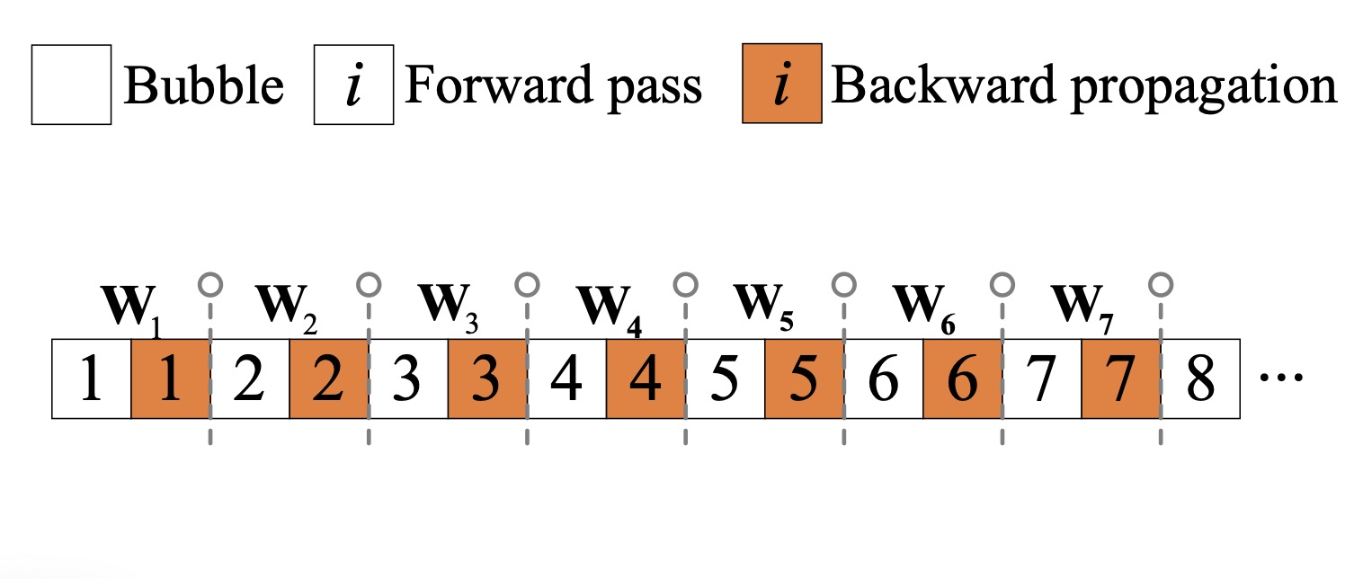
(a) Serial execution

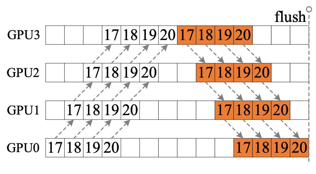
(b) GPipe

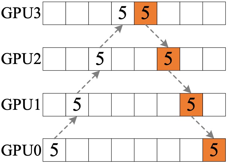
(c) Naive approach

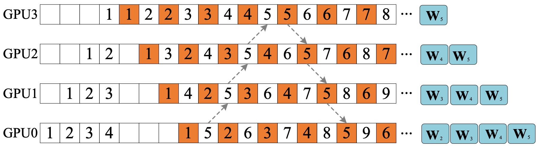
(d) PipeDream

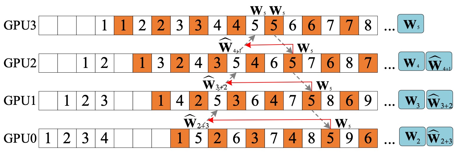
(e) PipeOptim

Figure 1: Timelines of serial execution, GPipe, Naive approach, PipeDream, and PipeOptim. In Figures 1(b), 1(c), 1(d), and 1(e), the grey dashed arrows depict the pipeline training of the 5th mini-batch. The blue squares on the right side of Figure 1(d) show the weights versions needed to be maintained during the training period of the 5th mini-batch. The blue squares located at the right side of Figure 1(e) illustrate the maintained weights for the forward pass of the 5th mini-batch.

III-A Weight prediction by PipeOptim

In the following, we discuss how to bridge the gap between $\mathbf{W}_{t}$ and $\hat{\mathbf{W}}_{t+s}$ given the type of the optimization method and the available variables.

III-A1 Weight prediction formula

Motivated by the weight prediction strategy proposed in XGrad [24], we construct the weight prediction formula of PipeOptim for asynchronous pipelined training. The basis of PipeOptim is on the observation that on each GPU, the weights of a stage are updated in a continuous manner and that the relative variation of the weights should reflect the trend of weight updates.

We first reconsider the weight updates of the serial execution shown in Figure 1(a). We assume that the weights of any $t$-th ($t\geq 1$) mini-batch is ${\mathbf{W}}_{t}$ and the learning rate is $lr$. Thus, in the following $s$ ($s\geq 1$) times of mini-batch training, the DNN weights are updated via

$$\mathbf{W}_{t+1}=\mathbf{W}_{t}-lr\cdot\Delta\mathbf{W}_{t},$$

$$\mathbf{W}_{t+2}=\mathbf{W}_{t+1}-lr\cdot\Delta\mathbf{W}_{t+1},$$

$$\cdots$$

$$\mathbf{W}_{t+s}=\mathbf{W}_{t+s-1}-lr\cdot\Delta\mathbf{W}_{t+s-1}.$$ (1)

When summing up all weight update equations shown in (1), we can immediately get

$$\mathbf{W}_{t+s}=\mathbf{W}_{t}-lr\cdot\sum_{i=t}^{t+s-1}\Delta\mathbf{W}_{i},$$ (2)

where $\Delta\mathbf{W}_{i}$ represents the relative increments of $\mathbf{W}_{i+1}$ over $\mathbf{W}_{i}$. Equation (2) illustrates that given the initial weights $\mathbf{W}_{t}$, $\mathbf{W}_{t+s}$ can be computed by letting $\mathbf{W}_{t}$ subtract the result of the learning rate timing the sum of $s$ continuous relative variation of the weights. Note that each relative variation of the weights (i.e., $\Delta\mathbf{W}_{i}$) should reflect the “correct” direction for updating the weights [24]. Therefore, one can replace $\sum_{i=t}^{t+s-1}\Delta\mathbf{W}_{i}$ with $s\cdot\Delta\mathbf{W}_{t}$ in an effort to approximately compute $\mathbf{W}_{t+s}$ for the case when $\mathbf{W}_{t}$, $lr$, and $\Delta\mathbf{W}_{t}$ are available only.

The above discussions directly generate the following weight prediction formula performed by each stage:

$$\hat{\mathbf{W}}_{t+s}\approx\mathbf{W}_{t}-lr\cdot s\cdot\Delta\mathbf{W}_{t},$$ (3)

where $\mathbf{W}_{t}$ are the given stage weights, $\hat{{\mathbf{W}}}_{t+s}$ represent the predicted weights for ${\mathbf{W}}_{t}$. For the weight prediction of PipeOptim, the parameter $s$ is always known as weight version differences which refers to the number of weight updates performed between the current pipeline unit and the future pipeline unit at which the mini-batch with index $t+s$ is ready to do backward propagation.

Given that ${\mathbf{W}}_{t}$ and $lr$ are available, our focus then turns to how to compute $s$ and $\Delta{\mathbf{W}}_{t}$ to predict the future weights $\hat{\mathbf{W}}_{t+s}$ when using Equation (3) as the weight prediction formula.

III-A2 Computation of $s$

As shown in Figure 1(e), the version difference $s$ is highly dependent on the number of stages (i.e., the pipeline depth) and the index of each stage. PipeOptim lets each GPU compute $s$ via

$$s=D-rank-1,$$ (4)

where $D$ refers to the pipeline depth and $rank$ is the index of a stage with $rank\in\{0,1,\dots,size-1\}$.

III-A3 Computation of $\Delta{\mathbf{W}}_{t}$

In Figure 1(a), we assume that the $t$-th mini-batch computes the gradients by $\mathbf{g}_{t}=\nabla f(\mathbf{W}_{t})$ where $f(\cdot)$ is the loss function. According to the conclusions drawn in XGrad [24], given the gradients of the stochastic objective corresponding to the $t$-th mini-batch, one can easily compute $\Delta\mathbf{W}_{t}$ according to the update rule of the used optimizer. Based on the results shown in Reference [24], we can easily calculate $\Delta{\mathbf{W}}_{t}$ according to the updated rule of the used optimizer. Table I presents detailed information about how to compute $\Delta{\mathbf{W}}_{t}$ when using the three most frequently used optimizers in deep learning including SGDM [18], Adam [21], and AdamW [22]. We note here that for SGDM, $u$ denotes the momentum factor and $\tau$ refers to the dampening for momentum. For Adam and AdamW, $\mathbf{m}_{t}$ denotes the biased first-moment estimate; $\mathbf{v}_{t}$ represents the biased second raw moment estimate; $\hat{\mathbf{m}}_{t}$ is the bias-corrected first-moment estimate; $\hat{\mathbf{v}}_{t}$ is the bias-corrected second raw moment estimates; ${\mathbf{g}}_{t}^{2}$ refers to element-wise square with $\mathbf{g}_{t}^{2}=\mathbf{g}_{t}\odot\mathbf{g}_{t}$; $\epsilon$, $\gamma$ and $\lambda$ are constant values.

To sum up, during the “1F1B” schedule shown in Figure 1(e), for any mini-batch with weights $\mathbf{W}_{t}$, PipeOptim lets each GPU perform the weight prediction ahead of the forward pass via

$$\hat{\mathbf{W}}_{t+s}=\mathbf{W}_{t}-lr\cdot s\cdot\Delta\mathbf{W}_{t},$$ (5)

where $lr$ is the learning rate, $s$ denotes the weight version difference, and $\Delta\mathbf{W}_{t}$ are computed based on the update rule of the used optimizer. The calculations of $\Delta\mathbf{W}_{t}$ when using SGDM, Adam, and AdamW are shown in Table I. We do not list the calculations of $\Delta\mathbf{W}_{t}$ for other optimizers due to limited space.

TABLE I: The calculation of $\Delta{\mathbf{W}}_{t}$ for SGDM, Adam, and AdamW.

Optimizer	$\Delta{\mathbf{W}}_{t}$
SGDM	$\begin{array}[]{ll}\quad\quad{\Delta\mathbf{W}}_{t}=\mathbf{v}_{t},\\ \textnormal{s.t.}\quad{\mathbf{v}}_{t}=u\cdot\mathbf{v}_{t-1}+(1-\tau)\cdot\mathbf{g}_{t}.\end{array}$
Adam	$\begin{array}[]{ll}\quad\quad{\Delta\mathbf{W}}_{t}=\frac{\hat{\mathbf{m}}_{t}}{\sqrt{\hat{\mathbf{v}}_{t}}+\epsilon},\\ \textnormal{s.t.}\ \left\{\begin{array}[]{ll}\mathbf{m}_{t}=\beta_{1}\cdot\mathbf{m}_{t-1}+(1-\beta_{1})\cdot\mathbf{g}_{t},\\ {\mathbf{v}}_{t}=\beta_{2}\cdot\mathbf{v}_{t-1}+(1-\beta_{2})\cdot\mathbf{g}_{t}^{2},\\ \hat{\mathbf{m}}_{t}=\frac{\mathbf{m}_{t}}{1-\beta_{1}^{t}},\\ \hat{\mathbf{v}}_{t}=\frac{\mathbf{v}_{t}}{1-\beta_{2}^{t}}.\\ \end{array}\right.\end{array}$
AdamW	$\begin{array}[]{ll}\quad\quad{\Delta\mathbf{W}}_{t}=\frac{\hat{\mathbf{m}}_{t}}{\sqrt{\hat{\mathbf{v}}_{t}}+\epsilon},\\ \textnormal{s.t.}\ \left\{\begin{array}[]{ll}{\mathbf{m}}_{t}=\beta_{1}\cdot\mathbf{m}_{t-1}+(1-\beta_{1})\cdot\mathbf{g}_{t},\\ \mathbf{v}_{t}=\beta_{2}\cdot\mathbf{v}_{t-1}+(1-\beta_{2})\cdot\mathbf{g}_{t}^{2},\\ \hat{\mathbf{m}}_{t}=\frac{\mathbf{m}_{t}}{1-\beta_{1}^{t}},\\ \hat{\mathbf{v}}_{t}=\frac{\mathbf{v}_{t}}{1-\beta_{2}^{t}}.\\ \end{array}\right.\end{array}$

III-B Comparision with asynchronous PMP approaches

In this section, we compare PipeOptim with other popular asynchronous PMP approaches including PipeDream, Pipedream-2BW, and SpecTrain. Table II summarizes the detailed features of each approach.

III-B1 PipeOptim vs. PipeDream & PipeDream-2BW

All the approaches adopt the “1F1B” schedule but use different strategies to ensure effective learning. PipeOptim uses an optimizer-dependent weight prediction technique while PipeDream & PipeDream-2BW employ a weight stashing technique. The weight stashing technique can guarantee that each mini-batch uses consistent weights to perform forward pass and backward propagation but leaves the staleness issue unsolved. In contrast, the optimizer-dependent weight prediction strategy adopted by PipeOptim can address both the inconsistency and staleness issues incurred by the “1F1B” schedule. Furthermore, the weight stashing technique consumes more weight memory than the weight prediction technique (up to $D$ versions of weights for PipeDream and 2 versions of weights for PipeDream-2BW). In contrast, PipeOptim lets each GPU maintain one to two versions of weights.

III-B2 PipeOptim vs. SpecTrain

Both PipeOptim and SpecTrain adopt the “1F1B” schedule and use the weight prediction technique to ensure effective learning of the model parameters. However, the weight prediction scheme used by SpecTrain is built dedicated based on the update rule of SGDM while the weight prediction scheme of PipeOptim dynamically varies with the optimizer used to train the DNN models. For SpecTain, the weight inconsistency and staleness issues are conditionedly solved because SpecTrain works well only when using the SGDM optimizer. As opposed to SpecTrain, the weight prediction formula of PipeOptim changes dynamically as the type of used optimizer which makes it behave well whatever optimizer is used to train the DNN model. In addition, SpecTrain requires each mini-batch to execute weight prediction twice, both in the forward pass and backward propagation. While PipeOptim only performs one-time weight prediction at the forward pass, leading to less computation cost.

TABLE II: Comparisons of PipeDream, PipeDream-2BW, SpecTrain, and PipeOptim.

Approaches	Work Scheduling	Effective Learning	Inconsistency Issue	Staleness Issue	Weights Memory∗
PipeDream	“1F1B”	weight stashing	solved	unsolved	[$M_{\theta}$, $D*M_{\theta}$]
PipeDream-2BW	“1F1B”	weight stashing	solved	unsolved	2$M_{\theta}$
SpecTrain	“1F1B”	SGDM-based weight prediction	conditioned solved†	conditioned solved †	$2*M_{\theta}$
PipeOptim	“1F1B”	optimizer-based weight prediction	solved	solved	[$M_{\theta},2*M_{\theta}$]

• $M_{\theta}$ denotes the memory consumption for storing a stage.

• SpecTrain only works well when using SGDM as the optimizer.

IV The PipeOptim Workflow

Algorithm 1 describes the workflow of PipeOptim on a multi-GPU computing node. By default, each GPU holds a single stage, takes charge of updating its parameters, and meets the one-to-one correspondence. During the pipelined training, each GPU works in parallel and executes the same workflow shown in Algorithm 1.

Algorithm 1 The workflow of PipeOptim

0:  $rank$, $D$, and $lr$.

1:  Initialize or load the stage weights ${\mathbf{W}}$.

2:  $t\leftarrow 1$.

3:  while Mini-batch remains do

4:     if $rank<D-1$ then

5:        Cache the current weight $\mathbf{W}_{t}$.

6:        Compute version difference $s$ using Eq. (4).

7:        Compute $\Delta\mathbf{W}_{t}$ using the formula shown in Table I.

8:        Compute the predicted weights $\hat{\mathbf{W}}_{t}$ using Eq. (5).

9:        Do forward pass using $\hat{\mathbf{W}}_{t+s}$.

10:        Recover the cached weights $\mathbf{W}_{t}$.

11:     else

12:        Do forward pass using $\mathbf{W}_{t}$.

13:     end if

14:     Do backward propagation using $\mathbf{W}_{t}$.

15:     $t\leftarrow t+1$

16:  end while

16:  ${\mathbf{W}}$

Before the pipelined training starts, each GPU should initialize the stage weights or directly load the stage weights before the pipeline starts (line 1). Then the index of the weights version is set with $t\leftarrow 1$ (line 2). Throughout the pipelined training, each GPU runs a loop until the mini-batch training finishes (lines 3 to 16). At each iteration, the forward pass and backward propagation are executed in turn. Note that weight prediction is only performed by the GPUs with $rank<D-1$ (lines 4-10). The last GPU directly uses ${\mathbf{W}}_{t}$ to do both forward pass and backward propagation (lines 12 and 14). For the previous $D-1$ GPUs, PipeOptim always lets each mini-batch use predicted future weights $\hat{\mathbf{W}}_{t+s}$ to compute the forward pass. Concretely, on each GPU, weight prediction always goes ahead of the forward pass, where the currently available weights should be cached first (line 5). Then the weight version difference should always be calculated using Equation (4) (line 6) and $\Delta{\mathbf{W}}_{t}$ should be calculated by a quick lookup of Table I (line 7). Following that, PipeOptim applies Equation (5) to compute the predicted weights $\hat{\mathbf{W}}_{t+s}$ (line 8), subsequently computing the forward pass with $\hat{\mathbf{W}}_{t+s}$ (Line 9). After the forward pass, the cached weights are first restored and used to perform the backward propagation for another mini-batch.

Note that PipeOptim can be easily implemented on top of the popular pipeline parallelism frameworks such as PipeDream [13] and GPipe [16]. We do not report the implementation details because this goes beyond the main contributions of this paper.

V Experimental Results

V-A Experimental Setup

We conducted the experiments using two computing platforms, referred to as Machine-A and Machine-B. Machine-A is configured with four Nvidia GeForce RTX 2080TI GPUs, each possessing 11 GB of GPU device memory, and is powered by two Intel(R) Xeon(R) Gold 5118 CPUs running at 2.30 GHz. On the other hand, Machine-B is equipped with four NVIDIA Tesla P100 GPUs, each having 16 GB of GPU device memory, and is driven by an Intel Xeon E5-2680 CPU operating at 2.40 GHz.

Datasets and Models. We used three tasks and four datasets in our experiments: 1) Image Classification, using the CIFAR-100 and the Tiny-ImageNet [29] datasets; 2) Machine Translation, using the WMT16 English to German (WMT En $\rightarrow$ De) dataset [30]; 3) Sentiment Analysis, using the IMDb Movie Review Sentiment Dataset [31]. The CIFAR-100 includes 60,000 32$\times$32 color images. All the images are grouped into 100 classes with 500 training images and 100 testing images per class. Meanwhile, each CIFAR image was normalized using mean=[0.491,0.482,0.447] and std=[0.247, 0.243,0.262]. The Tiny-ImageNet dataset consists of 200 classes each having 500 training images and 50 validation images. Each $64\times 64$ image was first scaled up to $224\times 224\times 3$, subsequently being normalized using mean=[0.485, 0.456, 0.406] and std=[0.229, 0.224, 0.225]. The IMDb Movie Review Sentiment Dataset encompasses a collection of 25,000 training movie reviews and an additional 25,000 testing reviews. Each review within the dataset has been labeled with a sentiment classification, specifically categorized as either positive or negative. We utilized the WMT16 En $\rightarrow$ De dataset, comprising 36 million sentence pairs for training, and employed the “newstest2014” set, which consists of 2,999 sentence pairs, for validation.

Eight different deep learning models are chosen as the benchmark DNN models spanning across three different applications: 1) AlexNet [32], 2) VGG-16 [33], 3) ResNet-101 [34], 4) GoogleNet [35], 5) Inception-V3 [36], 6) Residual LSTM [37], 7) Google Neural Machine Translation (GNMT) [4] with 8 LSTM layers (dubbed as GNMT-8), and 8) GNMT with 16 LSTM layers (dubbed as GNMT-16).

We used the three most popular optimizers including SGDM [18], Adam [21], and AdamW [22] to optimize the DNN weights. In particular, we used SGDM and AdamW for the image classification task, Adam and AdamW for the sentiment analysis task, and Adam for the machine translation task. Each optimizer was set with the default hyper-parameters. To be concrete, for SGDM, we set momentum with 0.9 and weight decay with $5e^{-4}$. Furthermore, we respectively set $\beta_{1}=0.9$ and $\beta_{2}=0.999$ for both Adam and AdamW.

Evaluating Approaches. In the experiments, we mainly compared PipeOptim with other four representative PMP approaches including GPipe [16], PipeDream [13], PipeDream-2BW [17], and SpecTrain [19]. For both PipeDream and PipeDream-2BW, we used the source code released on the GitHub. The code of SpecTrain is also public-available online. For a fair comparison, we implemented PipeOptim and GPipe [16] on top of the PipeDream implementation, which can isolate the impact on performance caused by different system implementations. The experiment code is available at https://github.com/guanleics/PipeOptim. Besides, the following two measures were taken to ensure a fair comparison. First, all the evaluated approaches adopted the model partitioning approach proposed in PipeDream [13] to divide the DNN models into four stages, with each stage being assigned on a GPU. Second, each approach employed the recomputation technique [16] to reduce the memory consumption of storing the intermediate activation and achieve high GPU memory utilization.

Here we note that PipeOptim can be easily scaled to Multi-Node Multi-GPU systems by combining with the data parallelism as PipeDream [13] and PipeDream-2BW [17] do. We did not explore the scalability of PipeOptim in the experiment as the main purpose of the experiments is to validate the effectiveness of our proposal for achieving effective parameter learning for the “1F1B” schedule. Therefore, we always evaluated each PMP approach on a single multi-GPU computing node with each GPU taking charge of training a stage and meeting the one-to-one correspondence.

V-B Accuracy

In this section, we make a comparison in terms of the obtained model accuracy. Since GPipe automatically reduces to the naive PMP approach when a mini-batch is not split into smaller micro-batches. To simulate the behavior of the naive approach and to isolate the effects of model partition, we trained GPipe with $T=1$ where $T$ denotes the number of micro-batches in a mini-batch. Furthermore, we regarded the experiment results of GPipe with $T=1$ as the baseline as GPipe is a synchronous pipeline approach and incurs no model accuracy drop. To verify the effectiveness of PipeOptim and its robustness to the used optimizers, we divided the experiments into three groups according to the type of the used optimizer. Table III summarizes the optimizer, models, and datasets used in each experiment group. In the first group, we used SGDM to optimize the CNN models including AlexNet, ResNet-101, and Inception-V3. In the second group, we used Adam to optimize Residual LSTM, GNMT-8, and GNMT-16. In the third group, we used AdamW to optimize VGG-16, GoogleNet, and Residual LSTM.

TABLE III: Summarization of optimizer, models, and datasets used in each experiment group.

Groups	Optimizer	Models	Dataset
Group-1	SGDM	AlexNet, ResNet-101, Inception-V3	Tiny-Imagenet
Group-2	AdamW	VGG-16, GoogleNet	CIFAR-100
		Residual LSMT	IMDb
Group-3	Adam	Residual LSTM	IMDb
		GNMT-8	WMT-16 En$\rightarrow$De

The experiments were conducted on Machine A with 11 GB of memory. In Group-1, we set SGDM with the momentum factor $\gamma$ set to 0.9 and weight decay set to 5e-4. We trained AlexNet, ResNet-101, and Inception-V3 on Tiny-ImageNet for 70 epochs with a mini-batch size of 56. The learning rate was set to 0.01 and divided by 10 at the 40th and 60th epochs respectively. In Group-2, we used AdamW to train VGG-16 and GoogleNet on CIFAR-100 for 120 epochs with a mini-batch size of 128. We initialized the learning rate with 0.001 and decreased it by a factor of 10 at the 90th epoch. Furthermore, we used AdamW to optimize Residual LSTM for 50 epochs with a mini-batch size of 256. In Group-3, we used Adam to optimize Residual LSTM for 50 epochs with a mini-batch size of 256. The initial learning rate was 0.001 and decayed with the polynomial scheduling strategy [38]. We also trained GNMT-8 on the WMT En $\rightarrow$ De dataset, using the Adam optimizer. We trained GNMT-8 for 8 epochs with a mini-batch size of 64 and a fixed learning rate of $3e^{-4}$.

Figures 2, 3, and 4 show the learning curves about accuracy versus epochs for Group-1, Group-2, and Group-3 respectively. Table IV summarizes the obtained maximum accuracy of each evaluated PMP approach. We can reach the following conclusions based on the experiment results.

First, Figures 2(a), 2(b), and 2(c) reveal that the learning curves of PipeOptim match well with that of GPipe when training CNNs using the SGDM as the optimizer. In contrast, PipeDream and PipeDream-2BW converge worse than GPipe and PipeOptim, illustrating their inferior effectiveness in learning parameters. The experiment results in Table IV show that GPipe performs the best when training AlexNet while PipeOptim obtains the best top-1 accuracy for training ResNet-101 and Inception-V3. Compared to PipeDream and PipeDream-2BW, PipeOptim achieves an average of 1.95% (up to 5.24%) and 1.76% (up to 3.12%) higher accuracy. Furthermore, PipeOptim demonstrates very comparable accuracy as SpecTrain, both of which perform consistently better than PipeDream and PipeDream-2BW. This result demonstrates that the weight prediction technique outperforms the weight stashing technique in terms of effective learning when using the SGDM as the optimizer.

Second, the learning curves shown in Figures 3(a), 3(b), and 3(c) again verify the effectiveness of PipeOptim when optimizing the DNN models using the AdamW optimizer. It shows that given the same epochs, PipeOptim (in red lines) attains higher accuracy than the other competitors. Table IV shows that PipeOptim achieves the best accuracy than the other PMP approaches including GPipe. PipeOptim obtains an average of 0.80% (up to 0.86%) accuracy improvement over GPipe. Compared to PipeDream and PipeDream-2BW, the averaged accuracy improvement is 1.0% (up to 1.56%) and 0.41% (up to 0.99%), respectively. The experiment results verify that the proposed optimizer-based weight prediction strategy helps boost the accuracy and, in particular, is more effective than the weight stashing technique when training the DNN models using the AdamW optimizer.

Figure 4(a) illustrates the experimental results when training Residual LSTM on IMDb. Figure 4(b) shows the experimental results when training GNMT-8 on WMT-16 En$\rightarrow$De dataset. Both use Adam as the optimizer. When training Residual LSTM, GPipe attains the best accuracy, PipeOptim and PipeDream rank second, and PipeDream-2BW ranks last. On training GNMT-8, PipeOptim converges fast at the beginning and finally attains the highest BLEU score (21.29 vs. 21.22, 21.04, and 21.20). This demonstrates that PipeOptim can guarantee effective parameter learning when using the Adam optimizer to train the DNN models.

Overall, the experiments demonstrate the effectiveness and robustness of PipeOptim. Significantly, SpecTrain exhibits effective performance under specific conditions, excelling only when SGDM is employed as the optimizer. Contrastingly, the performance of PipeOptim is independent of the type of the used optimizer, which is consistently better than that of PipeDream and PipeDream-2BW and is the most comparable (even slightly better) with that of GPipe.

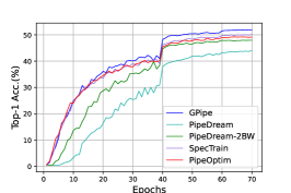
(a) AlexNet on Tiny-ImageNet

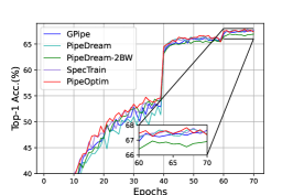
(b) ResNet-101 on Tiny-ImageNet

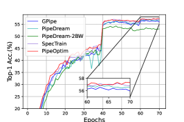
(c) Inception-V3 on Tiny-ImageNet

Figure 2: Experiment results of Group-1. Learning curves about top-1 accuracy versus epochs.

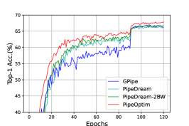
(a) VGG-16 on CIFAT-100

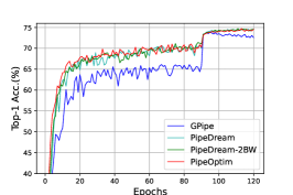
(b) GoogleNet on CIFAR-100

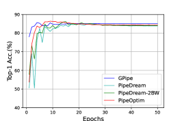
(c) Residual LSTM on IMDB

Figure 3: Experiment results of Group-2. Learning curves about top-1 accuracy versus epochs.

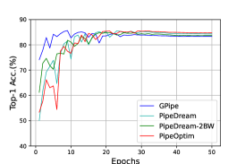
(a) Residual LSTM on IMDb

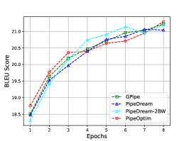
(b) GNMT-8 on WMT-16 En$\rightarrow$De

Figure 4: Experiment results of Group-3. Figure 4(a): top-1 accuracy versus epochs; Figure 4(b): BLEU score versus epochs.

TABLE IV: Summarization of obtained maximum model accuracy. The best results are highlighted in boldface.

Optimizer	Model	Dataset	Approaches
			GPipe	PipeDream	PipeDream-2BW	SpecTrain	PipeOptim
SGDM	AlexNet	Tiny-ImageNet	51.93%	43.99%	47.96%	50.14%	49.23%
	ResNet-101	Tiny-ImageNet	66.64%	67.72%	66.94%	67.81%	67.84%
	Inception-V3	Tiny-ImageNet	56.56%	56.88%	54.25%	57.13%	57.37%
AdamW	Residual LSTM	IMDB	85.65%	84.82%	86.15%	–	86.38%
	VGG-16	CIFAR-100	67.05%	66.61%	66.92%	–	67.91%
	GoogleNet	CIFAR-100	73.91%	74.58%	74.73%	–	74.73%
Adam	Residual LSTM	IMDB	85.64%	85.52%	84.88%	–	85.52%
	GNMT-8	WMT16	21.22 BLEU	21.04 BLEU	21.20 BLEU	–	21.29 BLEU

V-C Throughput

In this section, we compare the throughput of PipeOptim with that of GPipe, PipeDream, PipeDream-2BW, and SpecTrain. Note that to enable high throughput of GPipe, we evaluated the throughput of GPipe by splitting each mini-batch into 4 micro-batches as shown in Figure 1(b). We selected ResNet-101, GNMT-8, and GNMT-16 as the benchmark neural networks. We trained ResNet-101 on Tiny-ImageNet using the SGDM optimizer and trained GNMT-8 and GNMT-16 on WMT-16 En$\rightarrow$De using the Adam optimizer. The training setting was the same as described in Section V-B. The throughput for training ResNet-101 was defined as the number of training samples per second; while the throughput for training GNMT-8 and GNMT-16 was achieved by computing the number of the per-second training tokens within 1000 iterations.

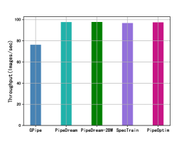
(a) ResNet-101

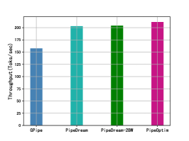
(b) GNMT-8

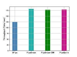
(c) GNMT-16

Figure 5: Throughput results when running with the same per-GPU batch size.

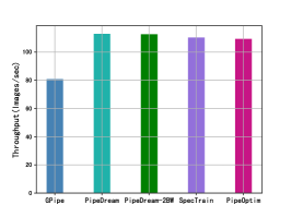
(a) ResNet-101

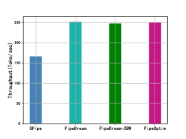
(b) GNMT-8

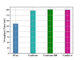
(c) GNMT-16

Figure 6: Throughput results when running with the maximum per-GPU batch size.

TABLE V: Summarization of maximum per-GPU mini-batch size.

Model	Dataset	Optimizer	GPipe	PipeDream	PipeDream-2BW	SpecTrain	PipeOptim
ResNet-101	Tiny-ImageNet	SGD	344/4=86	86	86	90	86
GNMT-8	WMT-16	Adam	520/4=130	136	140	–	142
GNMT-16	WMT-16	Adam	496/4=124	116	120	–	120

The experiments were conducted on Machine B with 16 GB of memory. We used two different strategies to compare the throughput of all the evaluated approaches. For the first strategy, we set each PMP approach with the same per-GPU batch size. Concretely, for PipeDream, PipeDream-2BW, SpecTrain, and PipeOptim, the per-GPU batch size for training ResNet-101, GNMT-8, and GNMT-16 were set to 64; while for GPipe, the mini-batch size was $64\times 4$. For the second strategy, we always selected an appropriate maximum per-GPU batch size so that each evaluated approach could run normally without yielding out-of-memory exceptions. It is worth noting that the experiments were conducted to compare the throughput of all evaluated approaches under the same experimental setting. All the evaluated approaches could consistently obtain higher throughput when a better model partition approach or elaborated hyper-parameter tuning is applied.

Figure 5 illustrates the throughput of all the evaluated approaches when filling Machine-B with the same per-GPU batch size. We can reach the following conclusions according to the experiment results. First, the experiment results shown in Figure 5 reveal that GPipe always generates the smallest throughput when training ResNet-101, GNMT-8, and GNMT-16. In contrast, the four asynchronous PMP approaches demonstrate much better throughput than GPipe, and at the same time, the throughput of these four PMP approaches is very comparable. Note that SpecTrain did not get a throughput result for training GNMT-8 and GNMT-16 because SpecTrain was unable to train GNMT using the Adam optimizer. This again demonstrates the significant limitations of SpecTrain. Meanwhile, the experimental results shown in Figure 5 demonstrate that PipeOptim always achieves pretty high throughput. When training ResNet-101, GNMT-8, and GNMT-16 with a fixed mini-batch size, PipeOptim achieves an average of 35% (up to 43%) throughput improvement over GPipe.

Figure 6 shows the throughput of all the evaluated approaches when filling Machine-B with the maximum per-GPU batch size. Table V summarizes the maximum mini-batch size of each PMP approach. Similar conclusions can be drawn according to the experiment results shown in Figure 6 and Table V. Again, GPipe obtains the lowest throughput among all evaluated PMP approaches. In particular, the experimental results depicted in Figure 6 again show that PipeOptim achieves consistently much higher throughput than GPipe. For training ResNet-101 with the maximum per-GPU mini-batch size, the throughput of PipeOptim exceeds that of GPipe by 35.3%. For training GNMT-8 and GNMT-16 with Machine-B, the averaged and maximum throughput improvement of PipeOptim over GPipe are 50.5% and 47.3% respectively. This gives rise to a throughput improvement of 44.37% on average. Meanwhile, the experimental results show that PipeOptim always obtains almost the same throughput as PipeDream and PipeDream-2BW. This demonstrates that the “1F1B” schedule is the main factor that contributes to the high throughput of the asynchronous PMP approaches. On the other hand, Table V demonstrates that each PMP approach always enjoys a comparable maximum per-GPU mini-batch size. In particular, compared to PipeDream, PIpeOptim, and PipeDream-2BW enable slightly larger mini-batch sizes when training GNMT-8 and GNMT-16. A larger batch size indicates less memory consumption for storing weight parameters. This phenomenon validates that PipeOptim and PipeDream-2BW require less GPU memory to store the weight parameters while PipeDream consumes the most GPU memory to store the weight parameters.

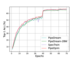
(a) Top-1 Accuracy vs. Epochs

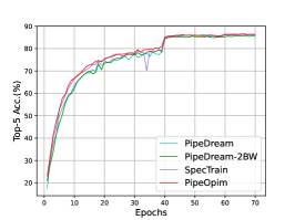
(b) Top-5 Accuracy vs. Epochs

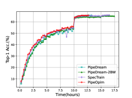
(c) Top-1 Accuracy vs. Time

Figure 7: Learning curves about training ResNet-101 using the SGDM optimizer.

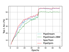
(a) Accuracy vs. Epochs

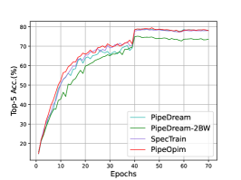
(b) Top-5 Accuracy vs. Epochs

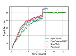
(c) Accuracy vs. Time

Figure 8: Learning curves about training Inception-V3 using the SGDM optimizer.

V-D Overall Performance

In this section, we evaluate and compare the overall performance of the asynchronous PMP approaches when simultaneously considering the convergence, throughput, and memory consumption. To be concrete, we trained each asynchronous PMP approach with a maximum per-GPU batch size so that they could run normally without yielding out-of-memory exceptions. The pipeline training was executed until reaching the threshold accuracy. We selected ResNet-101 and Inception-V3 as the benchmark model and conducted experiments on Machine-B. We trained ResNet-101 and Inception-V3 on Tiny-ImageNet using SGDM and followed the experiment setting described in Section V-B. Furthermore, we measured the overall performance of PipeOptim, PipeDream, PipeDream-2BW, and SpecTrain by training ResNet-101 and Inception-V3 until reaching the target top-1 accuracy of 66.0% and 55.5%.

Figures 7(a), 7(b), 8(a) and 8(b) show the learning curves about top-1/5 accuracy vs. epochs. Figures 7(c) and 8(c) depict the top-1 accuracy vs. running time until reaching the target accuracy. Table VI summarizes the experiment results about the overall performance. We can reach the following conclusions based on the observation of the experiment results. First, PipeOptim always obtains the best top-1 and top-5 accuracy. On average, the top-1 accuracy of PipeOptim exceeds PipeDream, PipeDream-2BW, and SpecTrain by an average of 0.12% (up to 0.17%), 3.15% (up to 4.99%), and 0.42% (up to 0.50%), respectively. In particular, we see that PipeDream-2BW performs the worst among all the asynchronous PMP approaches, even unable to achieve the target accuracy when training the Inception-V3. Second, each approach enjoys a very comparable 1-epoch running time, which demonstrates that the “1F1B” schedule is the main factor contributing to the training speed of the asynchronous PMP approaches. Third, thanks to its good convergence trait, PipeOptim requires the least running time to achieve the target accuracy. On training ResNet-101, PipeOptim yields a speedup of 1.04X, 1.37X, and 1.30X over PipeDream, PipeDream-2BW, and SpecTrain respectively. While for Inception-V3, the speedup of PipeOptim over PipeDream, PipeDream-2BW, and SpecTrain are 1.10X, $>$1.66X, and 1.10X.

TABLE VI: Results for overall performance evaluation. In this table, 1-epoch time stands for the average running time (in seconds) per epoch; total time refers to the total training time (in hours) to reach the target top-1 accuracy. The best results are highlighted in boldface.

Approach	Max. Top-1/5 Accuracy	1-epoch time	total time
ResNet-101
PipeDream	66.62% / 86.39%	918.15s	13.47h
PipeDream-2BW	65.39% / 85.71%	910.65s	17.67h
SpecTrain	66.19% / 86.33%	914.78s	16.77h
PipeOptim	66.69% / 86.57%	915.48s	12.91h
Inception-V3
PipeDream	55.74% / 78.91%	656.29s	8.57h
PipeDream-2BW	50.90% / 75.14%	663.19s	$>$12.91h
SpecTrain	55.57% / 78.63%	671.02s	8.57h
PipeOptim	55.91% / 79.48%	667.16s	7.76h

VI Related Work

Pipeline model parallelism has been recently intensively studied to reduce the communication volume and to increase the GPU utilization at the same time [39, 19, 40, 16, 13, 17, 41, 15, 42, 43]. GPipe [16] is the most influential synchronous PMP approach which ensures perfect convergence and incurs no accuracy drop but suffers from bubble overhead. After GPipe, many synchronous PMP approaches were proposed which share a common feature: reducing the bubble overhead by rescheduling the arrangement of mini-/micro-batches in the pipeline. For instance, GEMS [44] and Chimera [15] combine bidirectional pipelines with two versions of weights being simultaneously trained in the pipeline. DAPPLE [43] proposed an early backward scheduling strategy where the backward tasks were scheduled earlier and hence the memory used for storing activation produced by corresponding forward tasks is freed. For asynchronous pipeline training, the “1F1B” schedule is widely used in the popular asynchronous PMP approaches including PipeDream [13], PipeDream-2BW [17], and SpecTrain [19], where PipeDream and PipeDream-2BW make use of the weight stashing technique to achieve effective learning while SpecTrain adopts SGDM-based weight prediction to realize conditionally effective learning. Furthermore, PipeMare [41] improves the statistical efficiency of asynchronous pipeline parallelism by using the learning rate rescheduling and discrepancy correction. AvgPipe [45] proposes to use the elastic averaging technique [46] to maintain the statistical efficiency of the execution of multiple pipelines.

Pipeline model parallelism can be combined with data parallelism to scale pipeline parallelism from single computing nodes to multi-node-multi-GPU systems. Many popular PMP approaches such as PipeDream [13], PipeDream-2BW [17], Chimera [15], and DAPPLE [43] support this hybrid-parallel training manner. An alternative manifestation of hybrid parallelism involves simultaneously integrating data parallelism, tensor parallelism, and pipeline model parallelism. Examples of this approach include DistBelief [47] and Megatron-LM [48], which are specifically crafted for the training of large-scale deep neural network models.

VII Concluding remarks

In this work, we propose an efficient asynchronous PMP approach called PipeOptim. The key insight of PipeOptim is that it uses the optimizer-dependent weight prediction to simultaneously address the weight inconsistency and weight staleness issues incurred by the “1F1B” schedule. This directly gives rise to threefold innovations. First, PipeOptim can effectively handle the staleness issue that was left unsolved by the weight stashing technique of PipeDream and PipeDream-2BW, giving rise to better convergence and higher accuracy. Second, the efficiency of PipeOptim is independent of the used optimizer, contrasting sharply with SpecTrain which works well only when using the SGDM as the optimizer. Third, PipeOptim only requires each GPU to maintain up to two versions of weights.

Overall, PipeOptim achieves the best trade-off among GPU utilization, effective learning, and memory consumption. The experimental results demonstrate that PipeOptim outperforms PipeDream, PipeDream-2BW, and SpecTrain in terms of effective learning and, with quite comparable accuracy, heavily beats GPipe in in terms of GPU utilization. For example, when training Inception-V3 to the target accuracy, PipeOptim generates 1.10X, $>$1.66X, and 1.10X speedup over PipeDream, PipeDream-2BW, and SpecTrain, respectively. Our research paves a new way for efficient and effective asynchronous pipelined training.

References

- [1] A. Karpathy, G. Toderici, S. Shetty, T. Leung, R. Sukthankar, and L. Fei-Fei, “Large-scale video classification with convolutional neural networks,” in Proceedings of the IEEE conference on Computer Vision and Pattern Recognition, 2014, pp. 1725–1732.
- [2] N. Carion, F. Massa, G. Synnaeve, N. Usunier, A. Kirillov, and S. Zagoruyko, “End-to-end object detection with transformers,” in European Conference on Computer Vision. Springer, 2020, pp. 213–229.
- [3] H. Chen, Y. Wang, T. Guo, C. Xu, Y. Deng, Z. Liu, S. Ma, C. Xu, C. Xu, and W. Gao, “Pre-trained image processing transformer,” in Proceedings of the IEEE/CVF Conference on Computer Vision and Pattern Recognition, 2021, pp. 12 299–12 310.
- [4] Y. Wu, M. Schuster, Z. Chen, Q. V. Le, M. Norouzi, W. Macherey, M. Krikun, Y. Cao, Q. Gao, K. Macherey et al., “Google’s neural machine translation system: Bridging the gap between human and machine translation,” arXiv preprint arXiv:1609.08144, 2016.
- [5] A. Vaswani, N. Shazeer, N. Parmar, J. Uszkoreit, L. Jones, A. N. Gomez, Ł. Kaiser, and I. Polosukhin, “Attention is all you need,” Advances in neural information processing systems, vol. 30, 2017.
- [6] J. Devlin, M.-W. Chang, K. Lee, and K. Toutanova, “Bert: Pre-training of deep bidirectional transformers for language understanding,” arXiv preprint arXiv:1810.04805, 2018.
- [7] T. B. Brown, B. Mann, N. Ryder, M. Subbiah, J. Kaplan, P. Dhariwal, A. Neelakantan, P. Shyam, G. Sastry, A. Askell et al., “Language models are few-shot learners,” arXiv preprint arXiv:2005.14165, 2020.
- [8] T. Afouras, J. S. Chung, A. Senior, O. Vinyals, and A. Zisserman, “Deep audio-visual speech recognition,” IEEE transactions on pattern analysis and machine intelligence, 2018.
- [9] H. Lee, P. Pham, Y. Largman, and A. Y. Ng, “Unsupervised feature learning for audio classification using convolutional deep belief networks,” in Advances in neural information processing systems, 2009, pp. 1096–1104.
- [10] Y. Wang, A. Mohamed, D. Le, C. Liu, A. Xiao, J. Mahadeokar, H. Huang, A. Tjandra, X. Zhang, F. Zhang et al., “Transformer-based acoustic modeling for hybrid speech recognition,” in ICASSP 2020-2020 IEEE International Conference on Acoustics, Speech and Signal Processing (ICASSP). IEEE, 2020, pp. 6874–6878.
- [11] P. Goyal, P. Dollár, R. Girshick, P. Noordhuis, L. Wesolowski, A. Kyrola, A. Tulloch, Y. Jia, and K. He, “Accurate, large minibatch sgd: Training imagenet in 1 hour,” arXiv preprint arXiv:1706.02677, 2017.
- [12] Y. You, I. Gitman, and B. Ginsburg, “Scaling sgd batch size to 32k for imagenet training,” arXiv preprint arXiv:1708.03888, vol. 6, 2017.
- [13] D. Narayanan, A. Harlap, A. Phanishayee, V. Seshadri, N. R. Devanur, G. R. Ganger, P. B. Gibbons, and M. Zaharia, “Pipedream: generalized pipeline parallelism for dnn training,” in Proceedings of the 27th ACM Symposium on Operating Systems Principles. ACM, 2019, pp. 1–15.
- [14] G. Kwasniewski, M. Kabić, M. Besta, J. VandeVondele, R. Solcà, and T. Hoefler, “Red-blue pebbling revisited: near optimal parallel matrix-matrix multiplication,” in Proceedings of the International Conference for High Performance Computing, Networking, Storage and Analysis, 2019, pp. 1–22.
- [15] S. Li and T. Hoefler, “Chimera: efficiently training large-scale neural networks with bidirectional pipelines,” in Proceedings of the International Conference for High Performance Computing, Networking, Storage and Analysis, 2021, pp. 1–14.
- [16] Y. Huang, Y. Cheng, A. Bapna, O. Firat, D. Chen, M. Chen, H. Lee, J. Ngiam, Q. V. Le, Y. Wu et al., “Gpipe: Efficient training of giant neural networks using pipeline parallelism,” in Advances in Neural Information Processing Systems, 2019, pp. 103–112.
- [17] D. Narayanan, A. Phanishayee, K. Shi, X. Chen, and M. Zaharia, “Memory-efficient pipeline-parallel dnn training,” in International Conference on Machine Learning. PMLR, 2021, pp. 7937–7947.
- [18] N. Qian, “On the momentum term in gradient descent learning algorithms,” Neural networks, vol. 12, no. 1, pp. 145–151, 1999.
- [19] C.-C. Chen, C.-L. Yang, and H.-Y. Cheng, “Efficient and robust parallel dnn training through model parallelism on multi-gpu platform,” arXiv preprint arXiv:1809.02839, 2018.
- [20] T. Tieleman and G. Hinton, “Lecture 6.5-rmsprop: Divide the gradient by a running average of its recent magnitude,” COURSERA: Neural networks for machine learning, vol. 4, no. 2, pp. 26–31, 2012.
- [21] D. P. Kingma and J. Ba, “Adam: A method for stochastic optimization,” arXiv preprint arXiv:1412.6980, 2014.
- [22] I. Loshchilov and F. Hutter, “Decoupled weight decay regularization,” arXiv preprint arXiv:1711.05101, 2017.
- [23] L. Guan, “Adaplus: Integrating nesterov momentum and precise stepsize adjustment on adamw basis,” arXiv preprint arXiv:2309.01966, 2023.
- [24] L. Guan, D. Li, J. Meng, and Y. Shi, “Xgrad: Boosting gradient-based optimizers with weight prediction,” arXiv preprint arXiv:2305.18240, 2023.
- [25] R. Mayer and H.-A. Jacobsen, “Scalable deep learning on distributed infrastructures: Challenges, techniques, and tools,” ACM Computing Surveys (CSUR), vol. 53, no. 1, pp. 1–37, 2020.
- [26] M. Li, D. G. Andersen, J. W. Park, A. J. Smola, A. Ahmed, V. Josifovski, J. Long, E. J. Shekita, and B.-Y. Su, “Scaling distributed machine learning with the parameter server,” in 11th USENIX Symposium on operating systems design and implementation (OSDI 14), 2014, pp. 583–598.
- [27] P. Patarasuk and X. Yuan, “Bandwidth optimal all-reduce algorithms for clusters of workstations,” Journal of Parallel and Distributed Computing, vol. 69, no. 2, pp. 117–124, 2009.
- [28] T. Chen, B. Xu, C. Zhang, and C. Guestrin, “Training deep nets with sublinear memory cost,” arXiv preprint arXiv:1604.06174, 2016.
- [29] L. Yao and J. Miller, “Tiny imagenet classification with convolutional neural networks,” CS 231N, vol. 2, no. 5, p. 8, 2015.
- [30] R. Sennrich, B. Haddow, and A. Birch, “Edinburgh neural machine translation systems for wmt 16,” arXiv preprint arXiv:1606.02891, 2016.
- [31] A. Maas, R. E. Daly, P. T. Pham, D. Huang, A. Y. Ng, and C. Potts, “Learning word vectors for sentiment analysis,” in Proceedings of the 49th annual meeting of the association for computational linguistics: Human language technologies, 2011, pp. 142–150.
- [32] A. Krizhevsky, I. Sutskever, and G. E. Hinton, “Imagenet classification with deep convolutional neural networks,” Advances in neural information processing systems, vol. 25, 2012.
- [33] K. Simonyan and A. Zisserman, “Very deep convolutional networks for large-scale image recognition,” arXiv preprint arXiv:1409.1556, 2014.
- [34] K. He, X. Zhang, S. Ren, and J. Sun, “Deep residual learning for image recognition,” in Proceedings of the IEEE conference on computer vision and pattern recognition, 2016, pp. 770–778.
- [35] C. Szegedy, W. Liu, Y. Jia, P. Sermanet, S. Reed, D. Anguelov, D. Erhan, V. Vanhoucke, and A. Rabinovich, “Going deeper with convolutions,” in Proceedings of the IEEE conference on computer vision and pattern recognition, 2015, pp. 1–9.
- [36] C. Szegedy, V. Vanhoucke, S. Ioffe, J. Shlens, and Z. Wojna, “Rethinking the inception architecture for computer vision,” in The IEEE Conference on Computer Vision and Pattern Recognition (CVPR), June 2016.
- [37] J. Kim, M. El-Khamy, and J. Lee, “Residual lstm: Design of a deep recurrent architecture for distant speech recognition,” arXiv preprint arXiv:1701.03360, 2017.
- [38] P. Mishra and K. Sarawadekar, “Polynomial learning rate policy with warm restart for deep neural network,” in TENCON 2019-2019 IEEE Region 10 Conference (TENCON). IEEE, 2019, pp. 2087–2092.
- [39] A. L. Gaunt, M. A. Johnson, M. Riechert, D. Tarlow, R. Tomioka, D. Vytiniotis, and S. Webster, “Ampnet: Asynchronous model-parallel training for dynamic neural networks,” arXiv preprint arXiv:1705.09786, 2017.
- [40] T. Ben-Nun and T. Hoefler, “Demystifying parallel and distributed deep learning: An in-depth concurrency analysis,” arXiv preprint arXiv:1802.09941, 2018.
- [41] B. Yang, J. Zhang, J. Li, C. Ré, C. Aberger, and C. De Sa, “Pipemare: Asynchronous pipeline parallel dnn training,” Proceedings of Machine Learning and Systems, vol. 3, 2021.
- [42] C. He, S. Li, M. Soltanolkotabi, and S. Avestimehr, “Pipetransformer: Automated elastic pipelining for distributed training of large-scale models,” in International Conference on Machine Learning. PMLR, 2021, pp. 4150–4159.
- [43] S. Fan, Y. Rong, C. Meng, Z. Cao, S. Wang, Z. Zheng, C. Wu, G. Long, J. Yang, L. Xia et al., “Dapple: A pipelined data parallel approach for training large models,” in Proceedings of the 26th ACM SIGPLAN Symposium on Principles and Practice of Parallel Programming, 2021, pp. 431–445.
- [44] A. Jain, A. A. Awan, A. M. Aljuhani, J. M. Hashmi, Q. G. Anthony, H. Subramoni, D. K. Panda, R. Machiraju, and A. Parwani, “Gems: Gpu-enabled memory-aware model-parallelism system for distributed dnn training,” in SC20: International Conference for High Performance Computing, Networking, Storage and Analysis. IEEE, 2020, pp. 1–15.
- [45] Z. Chen, C. Xu, W. Qian, and A. Zhou, “Elastic averaging for efficient pipelined dnn training,” in Proceedings of the 28th ACM SIGPLAN Annual Symposium on Principles and Practice of Parallel Programming, 2023, pp. 380–391.
- [46] S. Zhang, A. E. Choromanska, and Y. LeCun, “Deep learning with elastic averaging sgd,” Advances in neural information processing systems, vol. 28, 2015.
- [47] J. Dean, G. Corrado, R. Monga, K. Chen, M. Devin, M. Mao, M. Ranzato, A. Senior, P. Tucker, K. Yang et al., “Large scale distributed deep networks,” Advances in neural information processing systems, vol. 25, 2012.
- [48] D. Narayanan, M. Shoeybi, J. Casper, P. LeGresley, M. Patwary, V. Korthikanti, D. Vainbrand, P. Kashinkunti, J. Bernauer, B. Catanzaro et al., “Efficient large-scale language model training on gpu clusters using megatron-lm,” in Proceedings of the International Conference for High Performance Computing, Networking, Storage and Analysis, 2021, pp. 1–15.