Heteroscedastic Uncertainty Estimation for Probabilistic Unsupervised Registration of Noisy Medical Images

Abstract

This paper proposes a heteroscedastic uncertainty estimation framework for unsupervised medical image registration. Existing methods rely on objectives (e.g. mean-squared error) that assume a uniform noise level across the image, disregarding the heteroscedastic and input-dependent characteristics of noise distribution in real-world medical images. This further introduces noisy gradients due to undesired penalization on outliers, causing unnatural deformation and performance degradation. To mitigate this, we propose an adaptive weighting scheme with a relative $\gamma$-exponentiated signal-to-noise ratio (SNR) for the displacement estimator after modeling the heteroscedastic noise using a separate variance estimator to prevent the model from being driven away by spurious gradients from error residuals, leading to more accurate displacement estimation. To illustrate the versatility and effectiveness of the proposed method, we tested our framework on two representative registration architectures across three medical image datasets. Our proposed framework consistently outperforms other baselines both quantitatively and qualitatively while also providing accurate and sensible uncertainty measures. Paired t-tests show that our improvements in registration accuracy are statistically significant. The code will be publicly available at https://voldemort108x.github.io/hetero_uncertainty/.

1 Introduction

Deformable image registration aims to learn a dense pixel-wise displacement map that shows the alignment between the moving and the fixed image. It is often a crucial step in medical image analysis that can help with screening disease progression and providing surgical guidance [12, 24]. Due to the practical difficulty of obtaining ground truth displacement, a number of classical methods propose iterative pair-wise optimization schemes using elastic-type models [10, 18], free-form deformation with b-splines [28], and diffeomorphic models [1, 2]. However, such methods are computationally expensive and impractical when facing large-scale real-world data.

With the recent advances in deep learning, a number of works formulate the problem in an unsupervised way by training a neural network to predict displacements between input image pairs without ground truth [4, 37, 7, 8, 30, 13, 16]. Such frameworks commonly utilize an unsupervised objective by minimizing the mean-square error (MSE) between the moved image (warped from the moving image using estimated displacement) and the fixed image. By using this objective, the existing frameworks assume additive white homoscedastic (uniform) Gaussian noise, i.e. $\epsilon\sim\mathcal{N}(0,\sigma^{2})$ with a constant noise variance across the image space. However, this assumption is especially problematic for medical images, where the noise is known to be often intrinsically heteroscedastic and input-dependent (e.g. MRI [33, 11] or ultrasound [36, 31, 23, 25]). The noise variance $\sigma_{I}^{2}(x)$ usually fluctuates non-uniformly across the image space as shown in Fig. 1 due to complicated factors such as changes in anatomical structures or patient motion during image acquisition. Using the simplified homoscedastic assumption disregards the variations of noise levels and will eventually result in undesired penalization on outliers, causing unnatural deformations and performance degradation.

Figure 1: (Motivation) Previous unsupervised image registration frameworks utilize an objective, such as mean-squared error [4, 7], that assumes homoscedastic noise across an image as shown in the left figure. This does not reflect the heteroscedastic and input-dependent characteristics of noise in real-world medical imaging data. To address this issue, we propose a heteroscedastic uncertainty estimation scheme as shown in the right figure to adaptively weigh the data-fidelity term accounting for the non-uniform variations of noise across the image.

A number of works were proposed to model heteroscedastic uncertainty in imaging problems [17, 29] but we argue that directly applying such frameworks to image registration will result in significant performance decline. This is due to that the heteroscedastic uncertainty estimation shares a distinct objective from image registration, and thus two modules cannot be optimized jointly.

To mitigate this, we propose a probabilistic heteroscedastic noise modeling framework for unsupervised image registration that adaptively learns the uncertainty characterized by noise to improve registration performance. Our proposed framework contains two modules: 1) a displacement estimator that predicts displacement within each image pair and 2) a variance estimator that models heteroscedastic noise (uncertainty) inside each image pair. To optimize our framework properly, we introduce a collaborative learning strategy that alternatingly optimizes a displacement estimator and variance estimator with separate objectives, avoiding the joint optimization issue mentioned above. We also propose an adaptive weighting strategy based on a relative $\gamma$-exponentiated signal-to-noise ratio using predictive heteroscedastic variance $\hat{\sigma}_{I}^{2}$ from the variance estimator to guide the displacement estimator to learn more accurate displacements. $\gamma$ reflects the confidence level of the current variance estimation. In order to validate the effectiveness of our proposed framework, we tested on three different cardiac datasets including 1) ACDC (public 2D MRI) [5], 2) CAMUS (public 2D ultrasound) [19], and 3) a private 3D echocardiography dataset (results shown in supplementary). To show the versatility of our proposed method, we implement our proposed framework on two representative registration architectures including 1) Voxelmorph [4] and 2) Transmorph ([7]). Our proposed framework can be operated in a plug-and-play manner to consistently improve registration performance in training while providing sensible heteroscedastic uncertainty measures to reflect spatially varying noise within each image pair. We also conducted paired t-tests to show that our improvements are statistically significant.

Contributions

• We propose a heteroscedastic uncertainty estimation framework for unsupervised image registration that extends the previous simplified homoscedastic assumption.

• We introduce an adaptive $\gamma$-exponentiated relative signal-to-noise weighting for displacement estimator during training to improve registration performance under the collaborative learning strategy together with a separate variance estimator.

• We demonstrate the effectiveness and versatility of our proposed framework on two representative registration architectures across three datasets with consistent statistically significant improvements over baselines while providing accurate uncertainty maps.

2 Related works

2.1 Unsupervised image registration

Balakrishnan et al. [4] proposed an unsupervised learning architecture by having a convolutional U-Net [27] to estimate displacement between moving and fixed images. The framework utilizes MSE as the unsupervised training objective assuming homoscedastic noise variance to update the network parameters. A number of works were developed upon this convolutional architecture including Voxelmorph-diff [9] with a probabilistic diffeomorphic architecture to model displacement uncertainty, Hypermorph [16] with an amortized hyperparameter optimization scheme, and Synthmorph [13] with a contrast-invariant design without acquired images.

To exploit the recent advances of transformers in vision tasks, Chen et al. [7] replaces the convolutional encoders in the Voxelmorph U-Net with swin transformer layers [20], termed TransUNet [6], to increase the receptive field of the encoding branch, potentially improving the long-range modeling capability. Several works explored based on this architecture including further replacing convolutional decoders with transformer layers [30] and introducing multi-scale image pyramids [21].

In this paper, we selected Voxelmorph [4] and Transmorph [7] as the representative registration architectures and tested our proposed framework and other baselines on both across different datasets. We also compared Voxelmorph-diff [9] with a direct extension of our framework by incorporating the heteroscedastic displacement uncertainty modeling as described in Sec. 6.3.

2.2 Heteroscedastic uncertainty estimation

To model the heteroscedastic uncertainty in imaging problems, Kendall and Gal [17] proposes a probabilistic joint optimization strategy by minimizing the negative log-likelihood (NLL) under the maximum likelihood estimation (MLE) framework via stochastic gradient descent. The objective includes a data-fidelity term with predictive inverse heteroscedastic variance weighting and a regularization term on the predictive variance. This formulation is proven to be effective in many applications such as surface normal estimation [3] and image segmentation [22]. Seitzer et al. [29] further advances such formulation by arguing that the inverse variance weighting on data fidelity results in undersampling, causing performance degradation. They propose a $\beta$-exponentiated weighting, termed $\beta$-NLL to address this issue. In this paper, we selected both NLL [17] and $\beta$-NLL [29] as our baselines for heteroscedastic uncertainty estimation.

2.3 Adaptive weighting schemes

A wide range of imaging problems is cast into optimizing an energy function, which contains a data-fidelity term and a regularization term. The relative importance between two terms is usually characterized by a scalar as a hyperparameter. However, such a strategy disregards the heteroscedastic nature of the error residuals [35]. To address this issue, several adaptive weighting schemes are proposed to weigh the data-fidelity term throughout optimization, accounting for non-uniform characteristics of the errors [14, 15, 34]. Wong et al. [35] later extends the above formulation to multi-frame setting. In this paper, we selected AdaReg [34] and AdaFrame [35] as baselines to compare with our proposed adaptive signal-to-noise weighting scheme.

3 Preliminary

Let $I:\Omega\rightarrow[0,1]$ be the imaging function with $x\in\Omega$ and $\Omega$ be the image space. Unsupervised image registration aims to find the alignment between moving image $I_{m}$ and fixed image $I_{f}$, characterized by a pixel-wise displacement vector field $z:\Omega\rightarrow\mathbb{R}^{2}$. For each image pair $(I_{m},I_{f})$, we assume $I_{m}$ is a fixed parameter and $I_{f}$ is a noisy observation of the warped image $\hat{I}_{f}=I_{m}\circ z$ with pixel-wise independence assumption with $\circ$ denoting image warping operation. Our goal is to solve for the posterior distribution $p(z|I_{f};I_{m})$ that will maximize the data likelihood $p(I_{f};I_{m})$ in an unsupervised way with no ground truth for $z$.

Since directly solving for $p(z|I_{f};I_{m})$ is intractable, we approximate it using a variational approach, where the approximate distribution is parameterized by a neural network $q_{\theta}(z|I_{f};I_{m})$, which we termed as displacement estimator. To minimize the distribution distance between our parameterized $q_{\theta}(z|I_{f};I_{m})$ and the real posterior $p(z|I_{f};I_{m})$, we compute the KL-divergence and arrive at the negative evidence lower bound:

$$\begin{split}&\text{KL}(q_{\theta}(z|I_{f};I_{m})\|p(z|I_{f};I_{m}))=\text{KL}(q_{\theta}(z|I_{f};I_{m})\|p(z))\\ &\qquad\qquad\qquad\qquad\;\;\;-\mathbb{E}_{q_{\theta}}(\log p(I_{f}|z;I_{m}))+\text{const.}\end{split}$$ (1)

The parameterized posterior is assumed to be a multivariate isotropic Gaussian with mean $\mu_{z}(x)\in\mathbb{R}^{2}$ and $\sigma_{z}^{2}\mathbb{I}\in\mathbb{R}^{2\times 2}$ as a diagonal scalar matrix, with $\mathbb{I}$ as the identity matrix

$$q_{\theta}(z|I_{f};I_{m})=\mathcal{N}(z;\mu_{z},\sigma_{z}^{2}\mathbb{I}).$$ (2)

To model the input-dependent heteroscedastic noise in the medical images, we assume a zero-meaned heteroscedastic Gaussian noise with spatially varying variance $\sigma_{I}^{2}(x)\in\mathbb{R}$

$$p(I_{f}|z;I_{m})=\mathcal{N}(I_{f};\hat{I}_{f},\sigma_{I}^{2}).$$ (3)

After further assuming the prior on $z$ is a zero-mean standard Gaussian $p(z)=\mathcal{N}(0,\mathbb{I})$, we arrive at the preliminary loss to be minimized for each image pair derived from Eq. 1 using assumptions Eq. 2 and Eq. 3 for each image pair

$$\mathcal{L}=\mathbb{E}_{\Omega}\left[\underbrace{\frac{1}{\sigma_{I}^{2}}\|I_{f}-\hat{I}_{f}\|_{2}^{2}}_{\mathcal{L}_{\text{data}}}+\log\sigma_{I}^{2}+\lambda\|\nabla z\|_{2}^{2}\right].$$ (4)

In the above equation, $\sigma_{I}^{2}$ is estimated by our proposed variance estimator $\hat{\sigma}_{I}^{2}=h_{\phi}(I_{f},\hat{I}_{f})$. Displacement $z$ is estimated by our displacement estimator as $\hat{z}=q_{\theta}(I_{m},I_{f})$.

4 Methods

4.1 Heteroscadestic uncertainty estimation using collaborative modeling

The preliminary loss defined in Eq. 4 implies the same objective to jointly update the parameters of both displacement estimator $q_{\theta}(\cdot)$ and variance estimator $h_{\phi}(\cdot)$. This may result in undersampling specific regions, particularly those with higher intensity profiles, as their noise variances tend to be elevated. This effect is observed in the displacement estimator within the image fidelity term $\mathcal{L}_{\text{data}}$ due to the application of absolute inverse variance weighting, further resulting in performance degradation. To mitigate this, we propose a collaborative learning strategy that separates the objective of the displacement estimator from the heteroscedastic variance estimation objective as shown in Fig. 2.

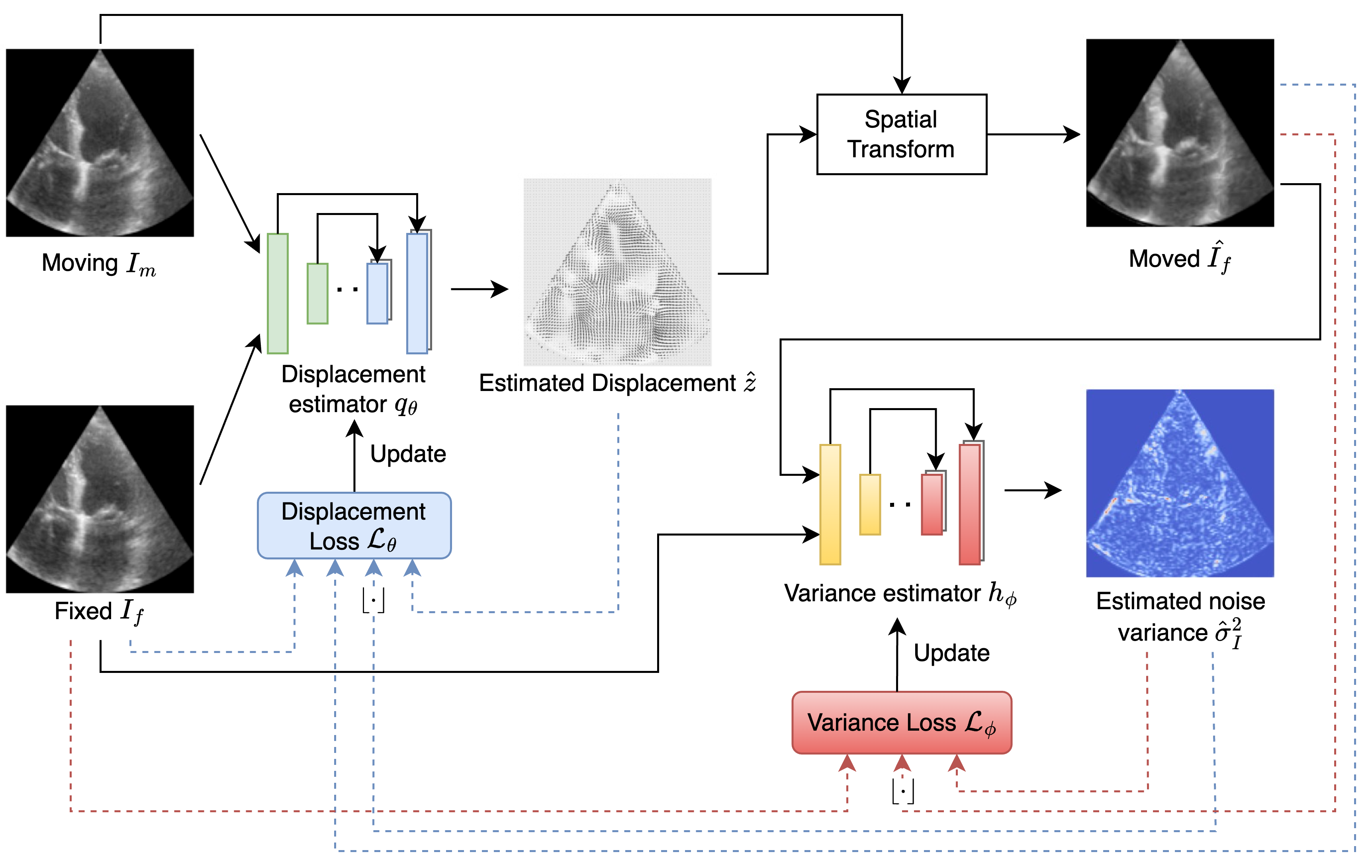
Figure 2: Overview of our proposed method. Our displacement estimator is built upon the U-Net backbone with final separate convolutional layers to predict the displacement. The noise variance estimator uses a similar U-Net backbone that takes reconstructed frame $\hat{I}_{f}$ along with frame $I_{f}$ to predict the heteroscedastic variance for the noise defined in Eq. 3.

In our proposed formulation (Fig. 2), the displacement and the variance estimators work collaboratively by using different objectives to update the network parameters while sharing intermediate predictions (i.e. estimated displacement $\hat{u}$ and variance $\hat{\sigma}_{I}^{2}$) to mutually enhance their performance. The displacement estimator parameters $\theta$ are updated using displacement loss, which is dependent on the quality of the predicted heteroscedastic variance by $h_{\phi}(\cdot)$. In parallel, the variance estimator update is also dependent on the quality of the reconstructed image (moved) warped using the displacement predicted by the displacement estimator. Both the displacement loss and the variance loss are elaborated in the following section.

4.2 Adaptive weighting using exponentiated relative signal-to-noise

Our proposed formulation in Section 4.1 offers the flexibility of designing customized objectives for displacement estimation and heteroscedastic variance estimation. Since the inverse-weighting strategy tends to be biased causing undersampling, we propose to weigh the image fidelity term based on the $\gamma$-exponentiated relative signal-to-noise ratio rather than the inverse of absolute variance. Our proposed displacement loss is defined as

$$\mathcal{L}_{\theta}=\mathbb{E}_{\Omega}\left[\mathcal{T}\left[\left(\frac{I_{f}}{\lfloor\hat{\sigma}_{I}\rfloor}\right)^{2\gamma}\right]\|I_{f}-\hat{I}_{f}\|_{2}^{2}+\lambda\|\nabla z\|_{2}^{2}\right],$$ (5)

where $\mathcal{T}(\cdot)$ is the sigmoid activation function. The exponentiated $\gamma$ indicates the confidence of the displacement model on the estimated heteroscedastic variance. When $\gamma=0$, the image reconstruction error reduces to MSE, showing that the displacement model is less confident in the variance estimate. When $\gamma=1$, the reconstruction error is weighted higher toward regions with relatively less noise. We experiment with different settings of $\gamma$ described in Sec. 6.4 and discover that a value of $\gamma=0.5$ achieves the optimal trade-off.

By stopping the gradient (denoted as $\lfloor\cdot\rfloor$) of the predicted heteroscedastic variance in displacement loss, the weighting term acts as an adaptive scalar map that encourages the network to concentrate on regions with relatively less noise, reducing the negative impact of undersampling.

For the variance estimator, we use the objective proposed by $\beta$-NLL [29] as our variance loss to update parameters $\phi$

$$\mathcal{L}_{\phi}=\mathbb{E}_{\Omega}\left[\lfloor\hat{\sigma}_{I}^{2\beta}\rfloor\left(\frac{1}{\hat{\sigma}_{I}^{2}}\|I_{f}-\lfloor\hat{I}_{f}\rfloor\|_{2}^{2}+\log\hat{\sigma}_{I}^{2}\right)\right].$$ (6)

We predict $\log\hat{\sigma}_{I}^{2}$ in our implementation as opposed to the absolute values for numerical stability.

4.3 Optimization of our proposed framework

In order to properly optimize our proposed framework, we propose a collaborative strategy with a warm-up stage followed by alternating optimization. The warm-up stage trains $N_{w}$ epochs individually for both estimators. This is particularly crucial during the initial stages of training, where both the displacement and variance estimators tend to provide inaccurate predictions. This initial inaccuracy can create a reciprocal negative influence between the two estimators, leading to a state of instability. The overall training procedure is summarized in Algorithm 1.

Data: Moving image $I_{m}$, fixed image $I_{f}$, learning rate $\eta$, warm-up epochs $N_{w}$.

Result: Displacement $z$ and heteroscedastic noise variance $\sigma_{I}^{2}$.

1

2for epoch $i=1$ to $N+2N_{w}$ do

3       if $i<N_{w}$ then

4             flag_disp = True, flag_variance = False;

5            

6      else

7             if $N_{w}\leq i<2N_{w}$ then

8                   flag_disp = False, flag_variance = True;

9                  

10            else

11                   flag_disp = True, flag_variance = True;

12                  

13            

14      

15      for step $j=1$ to $M$ do

16             if flag_disp then

17                   $\hat{z}=q_{\theta}(I_{m},I_{f})$;

18                   $\hat{I}_{f}=\text{SpatialTransform}(I_{m},z)$;

19                   if flag_variance then

20                         $\hat{\sigma}_{I}^{2}=h_{\phi}(I_{f},\hat{I}_{f})$;

21                        

22                  else

23                         $\hat{\sigma}_{I}^{2}=\mathbbm{1}$;

24                        

25                  $\mathcal{L}_{\text{disp}}=\mathcal{L}_{\theta}(I_{f},\hat{I}_{f},\lfloor\hat{\sigma}_{I}^{2}\rfloor,z)$;

26                   $\theta=\theta-\eta\nabla_{\theta}\mathcal{L}_{\text{disp}}$;

27                  

28            if flag_variance then

29                   $\hat{z}=q_{\theta}(I_{m},I_{f})$;

30                   $\hat{I}_{f}=\text{SpatialTransform}(I_{m},\hat{z})$;

31                   $\hat{\sigma}_{I}^{2}=h_{\phi}(I_{f},\hat{I}_{f})$;

32                   $\mathcal{L}_{\text{variance}}=\mathcal{L}_{\phi}(I_{f},\lfloor\hat{I}_{f}\rfloor,\hat{\sigma}_{I}^{2})$;

33                   $\phi=\phi-\eta\nabla_{\phi}\mathcal{L}_{\text{variance}}$;

34                  

35            

36      

Algorithm 1 Training procedure

5 Experiments and details

5.1 Datasets

We tested our method on three different cardiac datasets: (1) ACDC [5]: Human MRI, multiple 2D slices + time, 150 total sequences. (2) CAMUS [19]: Human echocardiography, 2D + time, 1000 total sequences from 500 patients, (3) Private 3D Echo: in vivo Porcine, in vivo canine, and synthetic echocardiography, 3D + time, 99 total sequences. The results of the private 3D Echo can be found in the supplementary. All datasets include segmentation of the left ventricular myocardium at the end-diastole (ED) and end-systole (ES) phases of the cardiac cycle. For all our following experiments, we aim to learn the displacement by warping ED to reconstruct ES (ED frame as moving and ES frame as fixed). We split the training, validation, and testing set by 60/20/20, randomly selected across the entire data. More details on the datasets and preprocessing steps can be found in the supplementary material.

5.2 Baselines

For each architecture (Voxelmorph [4], Transmorph [7]), we first follow the vanilla version by using objective $\mathcal{L}=\mathbb{E}_{\Omega}\left[\|I_{f}-\hat{I}_{f}\|_{2}^{2}+\lambda\|\nabla\hat{z}\|_{2}^{2}\right]$. We then replace the above objective with the following baselines.

5.2.1 Heteroscedastic uncertainty modeling

NLL [17]

We train our displacement and variance estimators jointly under the NLL objective: $\mathcal{L}_{\text{NLL}}=\mathbb{E}_{\Omega}\left[\frac{1}{\hat{\sigma}_{I}^{2}}\|I_{f}-\hat{I}_{f}\|_{2}^{2}+\log\hat{\sigma}_{I}^{2}+\lambda\|\nabla\hat{z}\|_{2}^{2}\right]$

$\beta$-NLL [29]

We train our displacement and variance estimators jointly under the $\beta$-NLL objective: $\mathcal{L}_{\beta\textrm{-NLL}}=\mathbb{E}_{\Omega}\left[\lfloor\hat{\sigma}_{I}^{2\beta}\rfloor\left(\frac{1}{\hat{\sigma}_{I}^{2}}\|I_{f}-\hat{I}_{f}\|_{2}^{2}+\log\hat{\sigma}_{I}^{2}\right)+\lambda\|\nabla\hat{z}\|_{2}^{2}\right]$ with $\beta=0.5$

5.2.2 Adaptive weighting schemes

AdaReg [34]

At each step, we first compute the local error residual $\rho=|I_{f}-\hat{I}_{f}|$ and the global residual $\sigma=\frac{1}{\mathbb{E}_{\Omega}[|I_{f}-\hat{I}_{f}|]}$ using the displacement estimator prediction $\hat{u}$. We then compute the adaptive regularization weighting as $\alpha=\exp(-\frac{c\rho}{\sigma})$, where $c=50$. We then optimize the displacement estimator and remove the variance estimator branch using the loss $\mathcal{L}_{\text{AdaReg}}=\mathbb{E}_{\Omega}\left[\|I_{f}-\hat{I}_{f}\|_{2}^{2}+\lambda\|\alpha\nabla\hat{z}\|_{2}^{2}\right]$.

AdaFrame [35]

At each step, we first compute the local error residual $\delta=|I_{f}-\hat{I}_{f}|$ and then normalize it with its mean $\mu$ and standard deviation $\sigma$ as $\rho=\frac{\delta-\mu}{\sqrt{\sigma^{2}+\epsilon}}$. We then compute the adaptive weight activated by a scaled and shifted sigmoid function as $\alpha=1-\frac{1}{1+\exp(-(a\rho-b))}$ where $a=\frac{a_{0}}{\mu+\epsilon}$ and $b=b_{0}(1-\cos\pi\mu)$. We choose $a_{0}=0.1$ and $b_{0}=10$. We then optimize the displacement estimator and remove the variance estimator branch using the loss $\mathcal{L}_{\text{AdaFrame}}=\mathbb{E}_{\Omega}\left[\alpha\|I_{f}-\hat{I}_{f}\|_{2}^{2}+\lambda\|\nabla\hat{z}\|_{2}^{2}\right]$.

5.3 Implementation details

All our experiments are conducted under the Pytorch framework and trained on NVIDIA V100/A5000 GPUs. The architecture of the variance estimator is implemented based on a U-Net. The remaining details including hyperparameters can be found in the supplementary.

6 Results

6.1 Registration accuracy

We present Tab. 1 to quantitatively evaluate the performance of our proposed method. As shown in the table, our proposed formulation consistently outperforms other baselines on each architecture across all datasets. This is also validated by the qualitative visualization as shown in Fig. 3, where our proposed method outperforms others by having smoother contour edges and locally consistent myocardial region. We also conducted paired t-tests to demonstrate that our improvements are statistically significant in Tab. 2. These results demonstrate the effectiveness and versatility of our proposed adaptive weighting based on relative signal-to-noise using the predictive variance from our proposed variance estimator.

ACDC [5] CAMUS [19] DSC $\uparrow$ HD $\downarrow$ ASD $\downarrow$ DSC $\uparrow$ HD $\downarrow$ ASD $\downarrow$ CNN Voxelmorph [4] 80.20 4.64 1.24 81.76 8.93 1.70 NLL [17] 76.49 5.46 1.45 75.24 11.05 2.20 $\beta$-NLL [29] 78.74 5.07 1.33 79.75 9.39 1.93 AdaFrame [35] 66.38 5.80 1.67 77.88 10.54 1.93 AdaReg [34] 78.75 5.13 1.33 79.31 9.78 1.88 Ours 80.73 4.57 1.21 81.96 8.80 1.66 Transformer Transmorph [7] 76.94 5.51 1.30 79.24 10.30 1.79 NLL [17] 73.12 7.22 1.27 75.08 11.60 1.79 $\beta$-NLL [29] 75.74 6.12 1.29 77.39 10.99 1.86 AdaFrame [35] 67.95 5.72 1.59 78.06 9.86 1.91 AdaReg [34] 76.22 5.68 1.29 78.12 10.62 1.84 Ours 78.12 5.04 1.26 80.38 9.86 1.72

Table 1: Contour-based metrics compared against baselines. DSC: Dice Similarity Coefficient (%). HD: Hausdorff Distance (vx). ASD: Average Surface Distance (vx). Our method consistently outperforms other baselines.

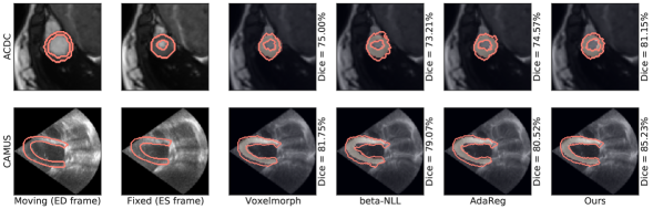
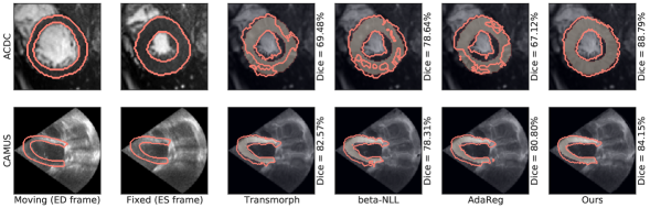
Figure 3: Qualitative evaluation of the registration accuracy via segmentation warping for all datasets (top two rows: Voxelmorph architecture [4], bottom two rows: Transmorph architecture [7]). Our method in the last column (overlayed with ground truth ES myocardium segmentation in yellow) predicts more natural and accurate deformations compared to baselines, evidenced by better matching with the ground-truth labels, smoother contour edges, and locally consistent myocardial region.

Voxelmorph [4] Transmorph [7] ACDC [5] $p<0.05$ $p<0.05$ CAMUS [19] $p<0.05$ $p<0.05$

Table 2: Paired t-tests of our proposed method v.s. the second-best method in Tab. 1 in terms of DSC. The $p$-values suggest that our improvements are statistically significant.

By comparing the results with the vanilla version of Voxelmorph [4] and Transmorph [7] in Tab. 1, we demonstrate the validity and necessity of modeling heteroscedastic noise in medical images, showing that not capturing spatially varying noise as in previous homoscedastic objective results in less accurate registration.

From Tab. 1, we also note that both NLL [17] and $\beta$-NLL failed to improve upon baselines, which validate our analysis in Sec. 4.1 that training displacement and displacement estimators jointly would degrade registration performance due to the undersampling resulted from inverse variance weighting. This also demonstrates the advantage of our proposed collaborative learning framework, which provides the flexibility of designing separate objectives for displacement and variance estimators as summarized in Algorithm 1, leading to superior performance. Furthermore, we observe that the adaptive weighting schemes including AdaReg [34] and AdaFrame [35] are ineffective in terms of improving the performance, which might be due to the statistical modeling of adaptive weights based on error residuals fails to represent complicated real-world data distribution. This also shows the advantage of our proposed data-driven adaptive weight based on SNR for displacement estimator.

6.2 Evaluation on heteroscedastic uncertainty

To quantitatively evaluate the accuracy of our estimated variance $\hat{\sigma}_{I}^{2}$, we utilized the sparsification error plots [26], which provide a numerical measure of the predicted uncertainty. To obtain such plots, we first rank pixels based on their corresponding estimated uncertainty magnitudes and then plot the reconstruction errors in terms of MSE of the remaining pixels ($\mathbb{E}_{\Omega-\Omega_{x}}\|I_{f}-\hat{I}_{f}\|_{2}^{2}$) versus the percentage of the removed pixels $\Omega_{x}$ based on the ranking [32]. A desired sparsification error plot from our setting should be monotonically decreasing given that the estimated uncertainty map is able to identify pixels that cause the largest errors. From Fig. 4, we show that the overall shape of the plots and the Area Under the Sparsification Error (AUSE) metrics both indicate that our estimated uncertainty is sensible across different datasets, with similar calibration levels compared to $\beta$-NLL [29] and better accuracy than NLL [17]. This illustrates the effectiveness of our proposed variance estimator and our proposed optimization framework summarized in Algorithm 1. We additionally tested on an alternative heteroscedastic Laplacian assumption shown in the supplementary.

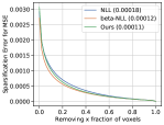
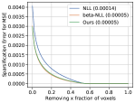
(1) ACDC [5]	(2) CAMUS [19]

Figure 4: Sparsification error plots of $\log\hat{\sigma}_{I}^{2}$ for all relevant methods and datasets. Our method has comparable uncertainty calibration to $\beta$-NLL [29] and better shape than NLL [17], showing the validity of our variance estimation.

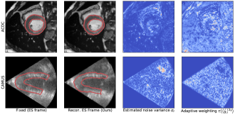
Figure 5: Estimated $\hat{\sigma}_{I}^{2}$ and the corresponding weighting map of our proposed framework under Voxelmorph architecture [4] (top row: ACDC [5]; bottom row: CAMUS [19]). Our predictive $\hat{\sigma}_{I}^{2}$ qualitatively makes sense since it correlates with the visual correspondence between the fixed image (first column) and the reconstructed image (second column) warped using estimated displacement. Our proposed weighting map also accurately reflects the relative importance between image intensity and predictive variance based on signal-to-noise, leading the displacement estimator to a better performance.

We further provide a qualitative visualization as shown in Fig. 5 on both datasets, where we demonstrate our estimated $\hat{\sigma}_{I}$ provides a sensible heteroscedastic noise variance map between the fixed image and reconstructed image according to our assumption. From the figure, our estimated noise variance shown in the third column reflects the intensity mismatches of the corresponding regions between fixed image $I_{f}$ in the first column and our reconstructed/moved image ($\hat{I}_{f}$) in the second column. This corroborates the validity of our heteroscedastic noise assumption Eq. 3 and shows the effectiveness of our proposed variance estimator. Furthermore, our computed adaptive weighting maps as shown in the last column of the figure accurately reflect the relative importance based on signal-to-noise, leading the displacement estimator to better registration performance.

6.3 Incorporating displacement uncertainty

Uncertainty ACDC [5] CAMUS [19] $\sigma_{z}^{2}$ $\sigma_{I}^{2}$ DSC $\uparrow$ HD $\downarrow$ ASD $\downarrow$ DSC $\uparrow$ HD $\downarrow$ ASD $\downarrow$ Vxm [4] ✗ ✗ 80.20 4.64 1.24 81.76 8.93 1.70 Vxm-diff [9] ✓ ✗ 76.19 5.75 1.19 76.74 10.76 1.88 Ours ✓ ✗ 79.80 4.74 1.22 81.47 8.67 1.69 Ours ✗ ✓ 80.73 4.57 1.21 81.96 8.80 1.66 Ours ✓ ✓ 79.87 4.62 1.20 81.91 8.54 1.65

Table 3: Our method raises the upper bound on registration accuracy while providing useful displacement uncertainty estimates $\hat{\sigma}_{z}$.

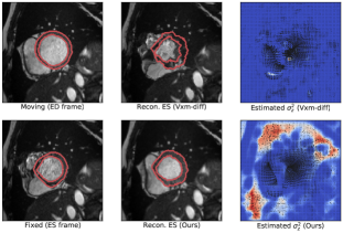
Figure 6: Estimated $\hat{\sigma}_{z}^{2}$ of our proposed method framework under Voxelmorph architecture [4] compared with Voxelmorph-diff [9]. The second column shows the warped images of both methods using the displacement predicted. We overlay our predicted $\sigma_{z}^{2}$ on estimated displacement $z$ in the third column where red indicates higher uncertainty and blue indicates lower. Our estimated $\sigma_{z}^{2}$ is able to capture the randomness more accurately in $z$ together with a better registration performance than Voxelmorph-diff when comparing the second column to the fixed image due to our proposed adaptive signal-to-noise weighting strategy.

To further demonstrate the versatility of our proposed framework, we conducted a direct extension by simultaneously estimating heteroscedastic displacement uncertainty under the isotropic assumption (uniform variance across image spatial dimensions). We add an additional layer in the displacement estimator to predict $\hat{\sigma}_{z}$, where $\hat{\sigma}_{z}(x)\in\mathbb{R}$ and the original prediction as displacement mean $\hat{\mu}_{z}$. We then train our proposed displacement estimator using objective $\mathcal{L}_{\theta}=\mathbb{E}_{\Omega}\left[\mathcal{T}\left[\left(\frac{I_{f}}{\lfloor\hat{\sigma}_{I}\rfloor}\right)^{2\gamma}\right]\|I_{f}-\hat{I}_{f}\|_{2}^{2}+\alpha\left(\hat{\sigma}_{z}^{2}-\log\hat{\sigma}_{z}^{2}\right)+\lambda\|\nabla z\|_{2}^{2}\right]$ derived from Eq. 1, with $\hat{z}$ sampled from the probabilistic distribution $\hat{z}\sim\mathcal{N}(\hat{\mu}_{z},\hat{\sigma}_{z}^{2}\mathbb{I})$ during training. In practice, we utilize the re-parameterization trick to avoid interruption in gradient-based optimization when doing the above sampling. We compare the quality of our predicted displacement along with its uncertainty estimate $\hat{\sigma}_{z}^{2}$ with the probabilistic diffeomorphic Voxelmorph (Voxelmorph-diff) [9]. We present our quantitative results in Tab. 3, illustrating the superiority of our formulation. We further present the qualitative visualization as shown in Fig. 6, demonstrating that our estimated heteroscedastic uncertainty $\hat{\sigma}_{z}^{2}$ accurately captures the randomness in the displacement prediction due to factors such as motion ambiguity. Additionally, we note that both our formulation and Voxelmorph as shown in Tab. 3 fail to improve registration performance by incorporating displacement uncertainty. We argue that by incorporating displacement uncertainty in both formulations does not contribute to learning a more accurate correspondence but rather provides an uncertainty estimate with the cost of accuracy, which results from the randomness in the sampling process in both frameworks ($\hat{z}\sim\mathcal{N}(\hat{\mu}_{z},\hat{\sigma}_{z}^{2}\mathbb{I})$) also degrades the performance.

6.4 Effect of $\gamma$

Uncertainty ACDC [5] CAMUS [19] $\sigma_{z}^{2}$ $\sigma_{I}^{2}$ DSC $\uparrow$ HD $\downarrow$ ASD $\downarrow$ DSC $\uparrow$ HD $\downarrow$ ASD $\downarrow$ Ours ($\gamma=0.25$) ✗ ✓ 79.74 4.74 1.26 82.07 8.53 1.65 Ours ($\gamma=0.5$) ✗ ✓ 80.73 4.57 1.21 81.96 8.80 1.66 Ours ($\gamma=0.75$) ✗ ✓ 80.00 4.69 1.24 81.82 8.45 1.66 Ours ($\gamma=1$) ✗ ✓ 79.78 4.71 1.25 81.31 9.08 1.69 Ours ($\gamma=0.25$) ✓ ✓ 79.68 4.65 1.21 81.63 9.17 1.65 Ours ($\gamma=0.5$) ✓ ✓ 79.87 4.62 1.20 81.91 8.54 1.65 Ours ($\gamma=0.75$) ✓ ✓ 79.01 4.71 1.22 81.52 8.64 1.67 Ours ($\gamma=1$) ✓ ✓ 80.20 4.92 1.16 81.01 8.75 1.72

Table 4: Effect of $\gamma$ in Eq. 5 for $\hat{\sigma}_{I}^{2}$ estimation (Sec. 6.2) and $\hat{\sigma}_{z}^{2}$ (Sec. 6.3) experiments. Although our method is not extremely sensitive to the choice of $\gamma$, we can still observe that $\gamma=0.5$ provides the best overall performance in terms of registration performance across all datasets.

As previously mentioned in Sec. 4.2, the exponentiated parameter $\gamma$ provides the flexibility to adjust the estimated $\hat{\sigma}_{I}^{2}$’s degree of influence on the displacement estimator during training. This can be viewed as a confidence trade-off in the current uncertainty estimate with $\gamma=0$ showing no confidence in current uncertainty estimation, reducing the adaptive weighting map to a uniform scalar map, and $\gamma=1$ indicating full belief. Considering the overall performance across all datasets, our method seems to perform best at $\gamma=0.5$ as shown in Tab. 4.

7 Conclusion

We propose a heteroscedastic uncertainty estimation framework for probabilistic unsupervised image registration to adaptively weigh the displacement estimation with relative $\gamma$-exponentiated signal-to-noise, which improves registration performance from the previously commonly used homoscedastic assumption while also provides accurate and sensible uncertainty measures. Our proposed framework consists of a displacement and a variance estimator, optimized under an alternating collaborative strategy. We demonstrate the effectiveness and versatility of our proposed framework on two representative registration architectures across diverse cardiac datasets and show consistent statistically significant improvements over other baselines. Though our proposed framework is promising, it still relies on a manually crafted adaptive map on the data fidelity term, which might not be able to fully reflect the complicated characteristics of large-scale real-world data. Future work will aim to explore a more data-driven objective with further validation of clinical datasets for more potential impact.

8 Acknowledgment

This work is supported by NIH grant R01HL121226.

Supplementary Material

9 Dataset details

9.1 ACDC [5]

The publicly available ACDC dataset contains 2D cardiac MRI scans from 150 patients with 100 subjects intended for training and 50 for testing. End-diastole (ED) and end-systole (ES) frames are identified in each sequence and corresponding myocardium labels are provided. We randomly selected 80 patients for training, 20 patients for validation, and 50 patients for testing. ED and ES image pairs are extracted from each sequence in a slice-by-slice manner from the 2D longitudinal stacks. We center crop each slice pair to $128\times 128$ w.r.t. myocardium centroid in ED frame. This yields 751 2D image pairs in total for training, 200 pairs for validation, and another 538 pairs for testing.

9.2 CAMUS [19]

The publicly available CAMUS dataset contains 2D cardiac ultrasound images from 500 subjects. Each subject contains 2 separate images including one for a 2-chamber view and another for a 4-chamber view. ED and ES frames along with myocardium segmentation labels are provided for each image. We resize each image pair to size $128\times 128$ and randomly select 300 subjects for training, 100 subjects for validation, and 100 subjects for testing. This yields in total 600 2D image pairs for training, 200 pairs for validation, and 200 pairs for testing.

9.3 Private 3D Echo

The private 3D echo dataset contains 99 cardiac ultrasound scans with 8 sequences from synthetic ultrasound, 40 sequences from in vivo canine, and another 51 sequences from in vivo porcine. The details of the acquisition are omitted to preserve anonymity in the review process. ED and ES frames are manually identified and myocardium segmentation labels are provided for each sequence by experienced radiologists. Each 3D image is resized to $64\times 64\times 64$. We randomly select 60 3D pairs for training, 19 pairs for validation, and another 20 pairs for testing.

10 Hyperparameter tuning

Parameters ACDC [5] CAMUS [19] Private 3D Echo $\lambda=0.1$ $\lambda=0.01$ $\lambda=0.001$ $\lambda=0.1$ $\lambda=0.01$ $\lambda=0.001$ $\lambda=0.1$ $\lambda=0.01$ $\lambda=0.001$ $\alpha=0.0001$ 70.53 79.77 77.64 74.02 80.76 79.63 70.78 73.85 72.97 $\alpha=0.00001$ 71.89 79.87 79.00 73.95 81.36 79.75 71.74 74.72 73.35 $\alpha=0.000001$ 70.77 78.53 78.65 75.74 81.91 80.22 73.27 73.96 73.28

Table 5: Effect of hyperparameter $\alpha$ and $\gamma$ of Sec. 6.3 evaluated using dice similarity coefficient (%).

Parameters ACDC [5] CAMUS [19] Private 3D Echo $\lambda=0.1$ $\lambda=0.01$ $\lambda=0.001$ $\lambda=0.1$ $\lambda=0.01$ $\lambda=0.001$ $\lambda=0.1$ $\lambda=0.01$ $\lambda=0.001$ $\alpha=0.0001$ 6.62 4.97 5.74 10.94 9.18 9.75 8.98 6.21 6.44 $\alpha=0.00001$ 5.18 4.62 5.12 17.57 9.28 9.31 10.24 5.79 5.99 $\alpha=0.000001$ 5.26 4.74 5.16 9.29 8.54 9.21 5.73 5.82 5.83

Table 6: Effect of hyperparameter $\alpha$ and $\gamma$ of Sec. 6.3 evaluated using Hausdorff distance (vx).

Parameters ACDC [5] CAMUS [19] Private 3D Echo $\lambda=0.1$ $\lambda=0.01$ $\lambda=0.001$ $\lambda=0.1$ $\lambda=0.01$ $\lambda=0.001$ $\lambda=0.1$ $\lambda=0.01$ $\lambda=0.001$ $\alpha=0.0001$ 1.09 1.04 1.23 1.68 1.48 1.65 0.76 0.86 0.88 $\alpha=0.00001$ 1.43 1.20 1.34 1.69 1.62 1.83 0.79 0.91 0.96 $\alpha=0.000001$ 1.51 1.26 1.36 2.06 1.65 1.83 0.91 0.96 0.98

Table 7: Effect of hyperparameter $\alpha$ and $\gamma$ of Sec. 6.3 evaluated using average surface distance (vx).

The learning rate of our proposed displacement and variance estimators is $1\times 10^{-4}$. For our proposed method, we choose $\lambda=0.01$. The effects of $\alpha$ and $\lambda$ in experiment Sec. 6.3 after incorporating displacement uncertainty are discussed in Tabs. 5, 6 and 7. From the tables, we note that $\alpha=0.01$ performs better overall, which is also consistent with our main results’ setting. For $\alpha$, we select $\alpha=0.00001$ for ACDC and our private 3D echo datasets, $\alpha=0.000001$ for CAMUS.

11 Alternative heteroscedastic noise assumption

Uncertainty ACDC [5] CAMUS [19] Private 3D Echo $\sigma_{z}^{2}$ $\sigma_{I}^{2}$ DSC $\uparrow$ HD $\downarrow$ ASD $\downarrow$ DSC $\uparrow$ HD $\downarrow$ ASD $\downarrow$ DSC $\uparrow$ HD $\downarrow$ ASD $\downarrow$ Laplacian Voxelmorph [4] ✗ ✗ 78.27 5.36 1.43 78.59 10.23 1.97 73.76 5.78 0.96 Voxelmorph-diff [9] ✓ ✗ 75.86 5.72 1.17 76.94 10.21 1.85 72.90 5.87 0.83 Ours ($\gamma=0.5$) ✓ ✗ 78.91 4.99 1.35 78.16 10.53 1.95 73.92 7.53 0.95 Ours ($\gamma=0.5$) ✓ ✓ 79.00 4.96 1.32 79.30 9.97 1.92 74.13 5.81 0.96 NLL [17] ✗ ✓ 76.00 5.88 1.47 75.10 11.21 2.18 72.91 6.13 0.97 $\beta$-NLL [29] ✗ ✓ 77.70 5.41 1.40 76.75 10.64 2.09 73.14 5.88 0.96 Ours ($\gamma=0.5$) ✗ ✓ 79.47 4.99 1.32 79.50 9.86 1.95 73.97 5.82 0.96

Table 8: Contour-based metrics compared against baselines under heteroscedastic Laplacian noise. DSC: Dice Similarity Coefficient (%). HD: Hausdorff Distance (vx). ASD: Average Surface Distance (vx). Our proposed framework using $\gamma$-exponentiated signal-to-noise weighting in the last row consistently outperforms other baselines.

Our preliminary loss defined in Eq. 3 described in Sec. 4.2 is based on a heteroscedastic Gaussian noise. To test the validity of this assumption, we conducted an additional analysis by replacing such an assumption with a heteroscedastic Laplacian noise. We repeat the experiments of our proposed framework and report quantitative results in the Tab. 8. From the table, our method as reported in the last row consistently outperforms other baselines across all three datasets. By comparing our main results reported in Tabs. 1 and 9, we observe that heteroscedastic Gaussian noise assumption achieves a better registration performance.

12 Private 3D Echo results

Private 3D Echo DSC $\uparrow$ HD $\downarrow$ ASD $\downarrow$ CNN Voxelmorph [4] 74.61 5.59 0.94 NLL [17] 72.59 6.35 0.97 $\beta$-NLL [29] 73.81 5.77 0.96 AdaFrame [35] 73.01 5.74 0.94 AdaReg [34] 73.41 5.91 0.95 Ours 75.04 5.55 0.93 Transformer Transmorph [7] 72.25 6.14 0.92 NLL [17] 67.98 6.97 0.85 $\beta$-NLL [29] 69.87 6.41 0.90 AdaFrame [35] 67.98 6.97 0.85 AdaReg [34] 69.87 6.41 0.90 Ours 71.38 6.11 0.95

Table 9: Quantitative evaluation of contour-based metrics compared against baselines on Private 3D Echo dataset. DSC: Dice Similarity Coefficient (%). HD: Hausdorff Distance (vx). ASD: Average Surface Distance (vx).

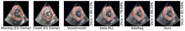
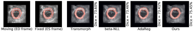
Figure 7: Qualitative evaluation of the registration accuracy via segmentation warping for our private 3D Echo dataset (top: Voxelmorph architecture [4], bottom: Transmorph architecture [7]). We extract cross-sectional slices from the 3D volume for visualization. Our method in the last column (overlayed with ground truth ES myocardium segmentation in yellow) predicts more natural and accurate deformations compared to baselines, evidenced by better matching with the ground-truth labels, smoother contour edges, and locally consistent myocardial region.

We present our qualitative result in Fig. 7, where we show that our proposed framework achieves a more accurate deformation compared to baselines, evidenced by better matching with the ground-truth labels, smoother contour edges, and locally consistent myocardial region. We present the quantitative evaluation with Tab. 9. We note that our proposed framework outperforms other baselines under the Voxelmorph architecture while achieving comparable performance with the vanilla version under the Transmorph architecture. This might be due to the size of our private 3D testing set being small with only 20 cases, which we will further evaluate on larger 3D in vivo animal datasets.

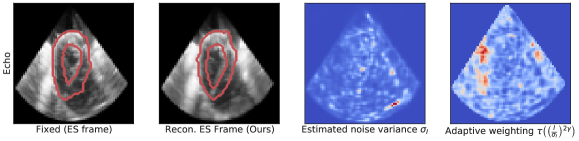
Figure 8: Estimated $\hat{\sigma}_{I}^{2}$ and the corresponding weighting map of our proposed framework under Voxelmorph architecture [4] using our private 3D Echo dataset. For visualization, we show the cross-sectional slice of the 3D volume. Our predictive $\hat{\sigma}_{I}^{2}$ qualitatively is sensible since it correlates with the visual correspondence between the fixed image (first column) and the reconstructed image (second column) warped using estimated displacement (e.g. bottom right image region in the third column). Our proposed weighting map also accurately reflects the relative importance between image intensity and predictive variance based on signal-to-noise, leading the displacement estimator to a better performance.

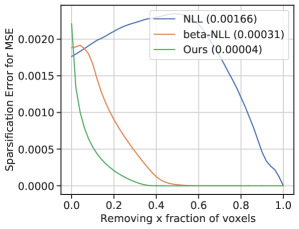
Figure 9: Sparsification error plots of $\log\hat{\sigma}_{I}^{2}$ for all relevant methods on our private 3D Echo dataset. Our method has better uncertainty calibration than both $\beta$-NLL [29] and NLL [17], showing the validity of our variance estimation.

To evaluate our estimated heteroscedastic noise variance qualitatively, we present Fig. 8. From the figure, we observe that our estimated noise variance $\hat{\sigma}_{I}$ is sensible since it visually correlates with regions that lack correspondence (e.g. bottom right region in the third column, where the correspondence does not exist in the first two columns). We also quantitatively evaluate the result by repeating the sparsification error plot similar to Sec. 6.2. We observe that our predicted $\hat{\sigma}_{I}$ achieves a better error curve than $\beta$-NLL and NLL, which is consistent with our main results shown in Fig. 4. We will further validate the effectiveness on larger in vivo animal datasets.

References

- Ashburner [2007] John Ashburner. A fast diffeomorphic image registration algorithm. NeuroImage, 38(1):95–113, 2007.
- Avants et al. [2008] B. B. Avants, C. L. Epstein, M. Grossman, and J. C. Gee. Symmetric diffeomorphic image registration with cross-correlation: Evaluating automated labeling of elderly and neurodegenerative brain. Medical Image Analysis, 12(1):26–41, 2008.
- Bae et al. [2021] Gwangbin Bae, Ignas Budvytis, and Roberto Cipolla. Estimating and Exploiting the Aleatoric Uncertainty in Surface Normal Estimation. In 2021 IEEE/CVF International Conference on Computer Vision (ICCV), pages 13117–13126, Montreal, QC, Canada, 2021. IEEE.
- Balakrishnan et al. [2019] Guha Balakrishnan, Amy Zhao, Mert R. Sabuncu, John Guttag, and Adrian V. Dalca. VoxelMorph: A Learning Framework for Deformable Medical Image Registration. IEEE Transactions on Medical Imaging, 38(8):1788–1800, 2019.
- Bernard et al. [2018] Olivier Bernard, Alain Lalande, Clement Zotti, Frederick Cervenansky, Xin Yang, Pheng-Ann Heng, Irem Cetin, Karim Lekadir, Oscar Camara, Miguel Angel Gonzalez Ballester, Gerard Sanroma, Sandy Napel, Steffen Petersen, Georgios Tziritas, Elias Grinias, Mahendra Khened, Varghese Alex Kollerathu, Ganapathy Krishnamurthi, Marc-Michel Rohe, Xavier Pennec, Maxime Sermesant, Fabian Isensee, Paul Jager, Klaus H. Maier-Hein, Peter M. Full, Ivo Wolf, Sandy Engelhardt, Christian F. Baumgartner, Lisa M. Koch, Jelmer M. Wolterink, Ivana Isgum, Yeonggul Jang, Yoonmi Hong, Jay Patravali, Shubham Jain, Olivier Humbert, and Pierre-Marc Jodoin. Deep Learning Techniques for Automatic MRI Cardiac Multi-Structures Segmentation and Diagnosis: Is the Problem Solved? IEEE Transactions on Medical Imaging, 37(11):2514–2525, 2018.
- Chen et al. [2021] Jieneng Chen, Yongyi Lu, Qihang Yu, Xiangde Luo, Ehsan Adeli, Yan Wang, Le Lu, Alan L. Yuille, and Yuyin Zhou. TransUNet: Transformers Make Strong Encoders for Medical Image Segmentation, 2021. arXiv:2102.04306 [cs].
- Chen et al. [2022] Junyu Chen, Eric C. Frey, Yufan He, William P. Segars, Ye Li, and Yong Du. TransMorph: Transformer for unsupervised medical image registration. Medical Image Analysis, 82:102615, 2022.
- Dalca et al. [2018] Adrian V. Dalca, Guha Balakrishnan, John Guttag, and Mert R. Sabuncu. Unsupervised Learning for Fast Probabilistic Diffeomorphic Registration. pages 729–738. 2018. arXiv:1805.04605 [cs].
- Dalca et al. [2019] Adrian V. Dalca, Guha Balakrishnan, John Guttag, and Mert R. Sabuncu. Unsupervised learning of probabilistic diffeomorphic registration for images and surfaces. Medical Image Analysis, 57:226–236, 2019.
- Davatzikos [1997] Christos Davatzikos. Spatial Transformation and Registration of Brain Images Using Elastically Deformable Models. Computer Vision and Image Understanding, 66(2):207–222, 1997.
- Eklund et al. [2017] Anders Eklund, Martin A. Lindquist, and Mattias Villani. A Bayesian heteroscedastic GLM with application to fMRI data with motion spikes. NeuroImage, 155:354–369, 2017.
- [12] Derek L G Hill, Philipp G Batchelor, Mark Holden, and David J Hawkes. Medical image registration.
- Hoffmann et al. [2022] Malte Hoffmann, Benjamin Billot, Douglas N. Greve, Juan Eugenio Iglesias, Bruce Fischl, and Adrian V. Dalca. SynthMorph: learning contrast-invariant registration without acquired images. IEEE Transactions on Medical Imaging, 41(3):543–558, 2022. arXiv:2004.10282 [cs, eess, q-bio].
- Hong et al. [2017a] Byung-Woo Hong, Ja-Keoung Koo, Martin Burger, and Stefano Soatto. Adaptive Regularization of Some Inverse Problems in Image Analysis, 2017a. arXiv:1705.03350 [cs].
- Hong et al. [2017b] Byung-Woo Hong, Ja-Keoung Koo, Hendrik Dirks, and Martin Burger. Adaptive Regularization in Convex Composite Optimization for Variational Imaging Problems, 2017b. arXiv:1609.02356 [cs].
- Hoopes et al. [2021] Andrew Hoopes, Malte Hoffmann, Bruce Fischl, John Guttag, and Adrian V. Dalca. HyperMorph: Amortized Hyperparameter Learning for Image Registration, 2021. arXiv:2101.01035 [cs, eess].
- Kendall and Gal [2017] Alex Kendall and Yarin Gal. What Uncertainties Do We Need in Bayesian Deep Learning for Computer Vision?, 2017. arXiv:1703.04977 [cs].
- Klein et al. [2010] S. Klein, M. Staring, K. Murphy, M.A. Viergever, and J. Pluim. elastix: A Toolbox for Intensity-Based Medical Image Registration. IEEE Transactions on Medical Imaging, 29(1):196–205, 2010.
- Leclerc et al. [2019] Sarah Leclerc, Erik Smistad, Joao Pedrosa, Andreas Ostvik, Frederic Cervenansky, Florian Espinosa, Torvald Espeland, Erik Andreas Rye Berg, Pierre-Marc Jodoin, Thomas Grenier, Carole Lartizien, Jan Dhooge, Lasse Lovstakken, and Olivier Bernard. Deep Learning for Segmentation Using an Open Large-Scale Dataset in 2D Echocardiography. IEEE Transactions on Medical Imaging, 38(9):2198–2210, 2019.
- Liu et al. [2021] Ze Liu, Yutong Lin, Yue Cao, Han Hu, Yixuan Wei, Zheng Zhang, Stephen Lin, and Baining Guo. Swin Transformer: Hierarchical Vision Transformer Using Shifted Windows. pages 10012–10022, 2021.
- Ma et al. [2023] Tai Ma, Xinru Dai, Suwei Zhang, and Ying Wen. PIViT: Large Deformation Image Registration with Pyramid-Iterative Vision Transformer. In Medical Image Computing and Computer Assisted Intervention – MICCAI 2023, pages 602–612, Cham, 2023. Springer Nature Switzerland.
- Monteiro et al. [2020] Miguel Monteiro, Loic Le Folgoc, Daniel Coelho de Castro, Nick Pawlowski, Bernardo Marques, Konstantinos Kamnitsas, Mark van der Wilk, and Ben Glocker. Stochastic Segmentation Networks: Modelling Spatially Correlated Aleatoric Uncertainty. In Advances in Neural Information Processing Systems, pages 12756–12767. Curran Associates, Inc., 2020.
- Nascimento and Marques [2008] Jacinto C. Nascimento and Jorge S. Marques. Robust Shape Tracking With Multiple Models in Ultrasound Images. IEEE Transactions on Image Processing, 17(3):392–406, 2008. Conference Name: IEEE Transactions on Image Processing.
- [24] Francisco P M Oliveira. Medical Image Registration: a Review.
- Ouzir et al. [2020] Nora Ouzir, Esa Ollila, and Sergiy A. Vorobyov. Data-Adaptive Similarity Measures for B-mode Ultrasound Images Using Robust Noise Models. IEEE Journal of Selected Topics in Signal Processing, 14(6):1244–1254, 2020. Conference Name: IEEE Journal of Selected Topics in Signal Processing.
- Poggi et al. [2020] Matteo Poggi, Filippo Aleotti, Fabio Tosi, and Stefano Mattoccia. On the Uncertainty of Self-Supervised Monocular Depth Estimation. In 2020 IEEE/CVF Conference on Computer Vision and Pattern Recognition (CVPR), pages 3224–3234, Seattle, WA, USA, 2020. IEEE.
- Ronneberger et al. [2015] Olaf Ronneberger, Philipp Fischer, and Thomas Brox. U-Net: Convolutional Networks for Biomedical Image Segmentation. In Medical Image Computing and Computer-Assisted Intervention – MICCAI 2015, pages 234–241, Cham, 2015. Springer International Publishing.
- Rueckert et al. [1999] D. Rueckert, L.I. Sonoda, C. Hayes, D.L.G. Hill, M.O. Leach, and D.J. Hawkes. Nonrigid registration using free-form deformations: application to breast MR images. IEEE Transactions on Medical Imaging, 18(8):712–721, 1999.
- Seitzer et al. [2022] Maximilian Seitzer, Arash Tavakoli, Dimitrije Antic, and Georg Martius. On the Pitfalls of Heteroscedastic Uncertainty Estimation with Probabilistic Neural Networks, 2022. arXiv:2203.09168 [cs, stat].
- Shi et al. [2022] Jiacheng Shi, Yuting He, Youyong Kong, Jean-Louis Coatrieux, Huazhong Shu, Guanyu Yang, and Shuo Li. XMorpher: Full Transformer for Deformable Medical Image Registration via Cross Attention, 2022. arXiv:2206.07349 [cs].
- Stanziola et al. [2019] Antonio Stanziola, Matthieu Toulemonde, Virginie Papadopoulou, Richard Corbett, Neill Duncan, Enrico Grisan, and Mengxing Tang. Sparse Image Reconstruction for Contrast Enhanced Cardiac Ultrasound using Diverging Waves. In 2019 IEEE International Ultrasonics Symposium (IUS), pages 908–911, Glasgow, United Kingdom, 2019. IEEE.
- Truong et al. [2021] Prune Truong, Martin Danelljan, Luc Van Gool, and Radu Timofte. Learning Accurate Dense Correspondences and When to Trust Them, 2021. arXiv:2101.01710 [cs].
- Wegmann et al. [2017] Bertil Wegmann, Anders Eklund, and Mattias Villani. Bayesian Heteroscedastic Regression for Diffusion Tensor Imaging. In Modeling, Analysis, and Visualization of Anisotropy, pages 257–282, Cham, 2017. Springer International Publishing.
- Wong and Soatto [2019] Alex Wong and Stefano Soatto. Bilateral Cyclic Constraint and Adaptive Regularization for Unsupervised Monocular Depth Prediction. In 2019 IEEE/CVF Conference on Computer Vision and Pattern Recognition (CVPR), pages 5637–5646, Long Beach, CA, USA, 2019. IEEE.
- Wong et al. [2021] Alex Wong, Xiaohan Fei, Byung-Woo Hong, and Stefano Soatto. An Adaptive Framework for Learning Unsupervised Depth Completion. IEEE Robotics and Automation Letters, 6(2):3120–3127, 2021.
- Zhang et al. [2021] Jingke Zhang, Qiong He, Yang Xiao, Hairong Zheng, Congzhi Wang, and Jianwen Luo. Ultrasound image reconstruction from plane wave radio-frequency data by self-supervised deep neural network. Medical Image Analysis, 70:102018, 2021.
- Zhang et al. [2022] Xiaoran Zhang, Chenyu You, Shawn Ahn, Juntang Zhuang, Lawrence Staib, and James Duncan. Learning Correspondences of Cardiac Motion from Images Using Biomechanics-Informed Modeling. In Statistical Atlases and Computational Models of the Heart. Regular and CMRxMotion Challenge Papers, pages 13–25, Cham, 2022. Springer Nature Switzerland.