Asymmetric Duffing oscillator: the birth and build-up of period doubling

Abstract

In this work, we investigate the period doubling phenomenon in the periodically forced asymmetric Duffing oscillator. We use the known steady-state asymptotic solution – the amplitude-frequency implicit function – and known criterion for the existence of period doubling. Working in the framework of differential properties of implicit functions we derive analytical formulas for the birth of period-doubled solutions.

1 Introduction and motivation

A period-doubling cascade of bifurcations is a typical route to chaos in nonlinear dynamical systems. We shall study this phenomenon in Duffing-type oscillator equations.

In this work, we study period doubling in the forced asymmetric Duffing oscillator governed by the non-dimensional equation:

$$\ddot{y}+2\zeta\dot{y}+\gamma y^{3}=F_{0}+F\cos\left(\Omega t\right),$$ (1)

which has a single equilibrium position and a corresponding one-well potential [1], where $\zeta$, $\gamma$, $F_{0}$, $F$ are parameters and $\Omega$ is the angular frequency of the periodic force.

The period doubling scenario in the dynamical system (1) was investigated by Szemplińska-Stupnicka in a series of groundbreaking papers [2, 3, 4], see also [1] for a review and further results.

The main idea introduced in [2] consists of perturbing the main steady-state asymptotic solution of Eq.(1), a $1:1$ resonance:

$$y_{0}\left(t\right)=A_{0}+A_{1}\cos\left(\Omega t+\theta\right),$$ (2)

as

$$y\left(t\right) = y_{0}\left(t\right)+u\left(t\right),$$ (3a)

$$u\left(t\right) = B\cos\left(\tfrac{1}{2}\Omega t+\varphi\right),$$ (3b)

substituting $y\left(t\right)$ into Eq.(1) and considering the condition of non-zero solution (3b). In papers [1, 2, 3, 4] several conditions guaranteeing the formation and stability of solution (3) were found and used to study the period doubling phenomenon.

For example, these authors were able to find intervals $\left(\Omega_{1},\ \Omega_{2}\right)$ in which solution (2) destabilized with the formation of period-doubled solution (3b) [1], and demonstrate that a cascade of period doubling leading to chaos was formed [1, 2, 3, 4].

Our motivation is fueled by the observation that steady-state solution (2 as well as period-doubling conditions found in [1, 2, 3, 4] are in the form of some implicit functions. Therefore, it should be possible, within the framework of differential properties of implicit functions [5], to obtain new results concerning the period-doubling mechanism.

The aim of the present work is thus to apply this formalism to implicit functions derived in [1, 2, 3, 4].

The paper is organized as follows. In Section 2 steady-state solution of Eq.(1) of form (2) is reviewed and a period doubling condition derived in [1, 2, 3, 4] is described in Section 3. In Section 4 we derive new results concerning period doubling applying the formalism of differential properties of implicit functions and in Section 5 we verify our results. In Section 6 we summarize our findings.

2 The main resonance: steady-state solution

The steady-state solution of Eq.(1) of form (2), describing $1:1$ resonance, was computed in Refs. [2, 6, 1]. Proceeding as in [7] we get two implicit equations for $A_{0},\ A_{1}$, and $\Omega$:

$$A_{1}^{2}\left(3\gamma A_{0}^{2}+\frac{3}{4}\gamma A_{1}^{2}-\Omega^{2}\right)^{2}+4\Omega^{2}\zeta^{2}A_{1}^{2} = F^{2},$$ (4a)

$$\gamma A_{0}^{3}+\frac{3}{2}\gamma A_{0}A_{1}^{2}-F_{0} = 0.$$ (4b)

Computing $$A_{1}^{2} A_{0}\neq 0 A_{0},\ \Omega$$ from Eq.(4b) for and substituting into (4a), we obtain finally one implicit equation for [1, 7]:

$$f\left(A_{0},\Omega;\gamma,\zeta,F_{0},F\right)=\sum\nolimits_{k=0}^{9}c_{k}A_{0}^{k}=0,$$ (5)

where the coefficients $c_{k}$ are given in Table 1 (cf. Eq.(8.3.12) in [1]).

Table 1: Coefficients $c_{k}$ of the polynomial (5)

$c_{9}=25\gamma^{3}$	$c_{4}=16\Omega^{2}\gamma F_{0}$
$c_{8}=0$	$c_{3}=-9\gamma F_{0}^{2}+6\gamma F^{2}$
$c_{7}=-20\Omega^{2}\gamma^{2}$	$c_{2}=-4F_{0}\Omega^{4}-16\zeta^{2}\Omega^{2}F_{0}$
$c_{6}=-15\gamma^{2}F_{0}$	$c_{1}=4\Omega^{2}F_{0}^{2}$
$c_{5}=4\gamma\Omega^{2}\left(\Omega^{2}+4\zeta^{2}\right)$	$c_{0}=-F_{0}^{3}$

We can also obtain an implicit equation for $A_{1},\ \Omega$ as in [7]. Solving Eq. (4b) for $A_{0}$ (there is only one real root) and substituting to (4a) we get:

$$g\left(A_{1},\Omega;\gamma,\zeta,F,F_{0}\right)=A_{1}^{2}\left(3\gamma A_{0}^{2}+\tfrac{3}{4}\gamma A_{1}^{2}-\Omega^{2}\right)^{2}+4\Omega^{2}\zeta^{2}A_{1}^{2}-F^{2}=0,$$ (6)

where $A_{0}$ and $Y$ are defined as:

$$A_{0}=-\frac{A_{1}^{2}}{2Y}+Y,\quad Y=\sqrt[3]{\sqrt{\frac{1}{8}A_{1}^{6}+\frac{1}{4\gamma^{2}}F_{0}^{2}}+\frac{1}{2\gamma}F_{0}}.$$ (7)

3 Birth of period doubling

The stability of the steady-state solution $y_{0}\left(t\right)=A_{0}+A_{1}\cos\left(\Omega t+\theta\right)$ is studied via a substitution in Eq. (1): $y=y_{0}+u\left(t\right)$, with $u\left(t\right)$ small. This substitution leads to the (linear) Hill’s equation for $u\left(t\right)$ [1, 2]:

$$\hat{L}u\equiv\ddot{u}+2\zeta\dot{u}+\left(\sigma_{0}+\sigma_{1}\cos\left(\Omega t+\theta\right)+\sigma_{2}\cos\left(2\left(\Omega t+\theta\right)\right)\right)u=0$$ (8a)

$$\sigma_{0}=3\gamma A_{0}^{2}+\dfrac{3}{2}\gamma A_{1}^{2},\quad\sigma_{1}=6\gamma A_{0}A_{1},\quad\sigma_{2}=\dfrac{3}{2}\gamma A_{1}^{2}$$ (8b)

provided that higher powers of $$u$$ are neglected.

To study destabilization of the $1:1$ resonance via the period doubling scenario one puts into Eq. (8):

$$u\left(t\right)=B\cos\left(\tfrac{1}{2}\Omega t+\varphi\right),$$ (9)

obtaining, after a harmonic balance method is used, a simple necessary condition for the onset of period-doubling (a condition for non-zero $B$):

$$h\left(A_{0},A_{1},\Omega;\gamma,\zeta\right)\equiv\left(\sigma_{0}-\frac{1}{4}\Omega^{2}\right)^{2}+\zeta^{2}\Omega^{2}-\frac{1}{4}\sigma_{1}^{2}=0,$$ (10)

see Eq. (8.5.5) in [1] or Eq. (4d) in [2].

Equation (10) can be simplified. We compute $A_{1}^{2}$ from Eq.(4b) for $A_{0}\neq 0$ and substitute into (10) obtaining a simplified condition for the birth of period doubling:

$$\left.\begin{array}[]{l}k\left(A_{0},\Omega;\gamma,\zeta,F_{0}\right)=10\gamma^{2}A_{0}^{6}-\gamma\Omega^{2}A_{0}^{4}-2\gamma F_{0}A_{0}^{3}\vskip 3.0pt plus 1.0pt minus 1.0pt\\ +\left(\tfrac{1}{16}\Omega^{4}+\zeta^{2}\Omega^{2}\right)A_{0}^{2}-\tfrac{1}{2}F_{0}\Omega^{2}A_{0}+F_{0}^{2}=0.\end{array}\right.$$ (11)

4 Differential condition for period doubling

We are going to show that there is a differential condition that permits a further insight into the nature of the birth of period doubling.

We consider a quite obvious differential condition for the birth of period doubling. More precisely, we investigate when equations (5), (11) have a common (real) root $\left(A_{0},\ \Omega\right)$. Suppose that the implicit function (11) has a singular point, an isolated point. Then equation (5) guarantees that this isolated point lies on the $1:1$ resonance amplitude-frequency curve (5) – a double solution of Eqs. (5), (11). This corresponds to a birth of instability of the $1:1$ resonance with the creation of period doubled solution (3b), i.e. to a birth of period doubling.

Accordingly, we consider the following equations:

$$f\left(A_{0},\Omega;\gamma,\zeta,F_{0},F\right) =0,$$ (12a)

$$k\left(A_{0},\Omega;\gamma,\zeta,F_{0}\right) =0,$$ (12b)

$$\frac{\partial k\left(A_{0},\Omega;\gamma,\zeta,F_{0}\right)}{\partial A_{0}} =0,$$ (12c)

$$\frac{\partial k\left(A_{0},\Omega;\gamma,\zeta,F_{0}\right)}{\partial\Omega} =0,$$ (12d)

where Eq.(12a), equivalent to (5), is the steady-state condition for $1:1$ resonance, Eq.(12b) is the period doubling condition (11 ) and equations (12c), (12d) mean that the implicit function (11) has a singular point. We show below that this singular point is an isolated point of (11).

Acceptable solutions of Eqs.(12), i.e $\Omega>0$, $A_{0}>0$, $\gamma>0$, $F>0$:

$$\Omega_{\ast}$$

   (13a)

where $$\zeta>0 F_{0}>0$$, are free parameters and

$$\begin{array}[]{ll}c_{1}=2\sqrt{2}\sqrt{\sqrt{2}+1}\cong 4.\,395,&c_{2}=\frac{3}{4}\left(1-\frac{1}{2}\sqrt{2}\right)\cong 0.\,220,\\ c_{3}=\frac{32}{27}\left(7\sqrt{2}+10\right)\cong 23.\,585,&c_{4}=\frac{3}{8}\sqrt{2}\sqrt{16\sqrt{2}+73}\cong 5.\,186,\end{array}$$ (13b)

have been computed using Maple from Scientific WorkPlace 4.0. Finally, we compute $A_{1\ast}^{2}$ from Eqs.(4b), (13a) and check that inequality $A_{1\ast}^{2}>0$ is fulfilled for $F_{0}>0$ since $\frac{3}{2}\gamma A_{0\ast}A_{1\ast}^{2}=F_{0}-\gamma_{\ast}A_{0\ast}^{3}=\frac{3}{4}F_{0}>0$.

Now we demonstrate that solution (13) corresponds to an isolated point. The determinant of the Hessian matrix, computed for the function $k\left(A_{0},\Omega;\zeta,\gamma,F_{0}\right)$ at singular point (13), is positive:

$$\det\left(\begin{array}[]{cc}\frac{\partial^{2}k\left(A_{0},\Omega\right)}{\partial\Omega^{2}}&\frac{\partial^{2}k\left(A_{0},\Omega\right)}{\partial\Omega\partial A_{0}}\vskip 3.0pt plus 1.0pt minus 1.0pt\\ \frac{\partial^{2}k\left(A_{0},\Omega\right)}{\partial A_{0}\partial\Omega}&\frac{\partial^{2}k\left(A_{0},\Omega\right)}{\partial A_{0}^{2}}\end{array}\right)=\left(36\sqrt{2}+18\right)\zeta^{2}F_{0}^{2}>0,$$ (14)

and this means that this is an isolated point [8].

For example, if we choose $\gamma=0.1$ and $\ F_{0}=0.02$ then we compute from Eqs. (13) other parameters, $\zeta$, $F$, as well as $\Omega$, $A_{0}$, and $A_{1}$ from Eq. (4b).

$$\zeta_{\ast}$$

(15)

And indeed, if we solve Eqs. (12a), (12b) for this set of parameters we obtain a double solution $\left(A_{0\ast},\ \Omega_{\ast}\right)=\left(0.479\,923,\ 0.368\,403\right)$, see also Fig.1, where the singular point $\left(A_{0\ast},\ \Omega_{\ast}\right)$ – an isolated point of implicit function (11 – is shown as a red dot.

For $\zeta>\zeta_{\ast}$ solutions of Eq. (12b) are complex, for $\zeta=\zeta_{\ast}$ there is a real isolated point lying on the curve (12a) – a red dot in Fig. 1, and for decreasing values of $\zeta$ curves (12b) are growing blue ovals. More exactly, in Fig. 1 in all cases, we have $\gamma=0.1$, $F_{0}=0.02$, $F=0.103\,721$ while $\zeta=0.109\,204$ (singular), $0.109$, $0.108$, $0.105$, $0.100$.

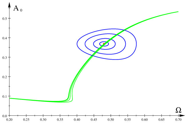
Figure 1: Implicit functions: (12a) (green), (12b) (blue), isolated point (red); $\gamma=0.1$, $F_{0}=0.02$, $F=0.103\,721$ and $\zeta=0.109\,204$ (singular), $0.109$, $0.108$, $0.105$, $0.100$.

Note that for decreasing $\zeta$ implicit function (12a), describing the $1:1$ resonance changes only slightly while the implicit function (12b), destabilization condition of the resonance, changes significantly.

5 Numerical verification

It follows from Section 4 that for $\gamma=0.1$, $F_{0}=0.02$, $F=0.103\,721$ destabilization of the $1:1$ resonance occurs for $\zeta\leq\zeta_{\ast}=0.109\,204$. Therefore, we have computed bifurcation diagrams solving Eq. (1) for $\gamma=0.1$, $F_{0}=0.02$, $F=0.103\,721$, and $\zeta\approx 0.109\,204$ looking for an onset of period doubling. And indeed, the resonance $1:1$ becomes unstable for $\zeta\cong 0.1105$.

Numerical solutions $y\left(t\right)$ of Eq. (1) (bifurcation diagrams) were computed running DYNAMICS [9] in the interval $\Omega\in\left(0.43,\ 0.70\right)$ for $\gamma=0.1$, $F_{0}=0.02$, $F=0.103\,721$ and $\zeta=0.1105$, $0.0621$, $0.0562$, $0.0550$, see Fig. 2.

We note that destabilization of the $1:1$ resonance with the formation of $1:2$ solution (3) (as well as other resonances) appears at $\Omega\approx 0.48$ in good agreement with the analytical value $\Omega_{\ast}=0.479\,923$ in 15.

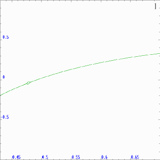
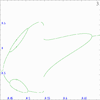
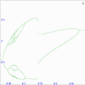
Figure 2: Bifurcation diagrams: $y$ (vertical axis) against $\Omega$ (horizontal axis), $\gamma=0.1$, $F_{0}=0.02$, $F=0.103\,721$ and $\zeta=0.1105$, $0.0621$, $0.0562$, $0.0550$ in diagrams $1$, $2$, $3$, $4$, respectively.

Moreover, we have computed numerical values of parameter $\zeta$ at which the first and subsequent period-doubling bifurcations occur, see Eq. (16). The first period doubling takes place at $\zeta=0.110\,533\,4$ in good agreement with analytical value $\zeta_{\ast}=0.109\,204$, see Eq. (15). We have also computed ratios $\dfrac{\zeta_{i-1}-\zeta_{i-2}}{\zeta_{i}-\zeta_{i-1}}$ which converge quite well to the Feigenbaum constant $\delta=4.669\,2011\,609\,\ldots$ [10].

$$i$$

(16)

6 Summary

Based on the known steady-state solution (2), (4) and period doubling-condition (10) (or simplified Eq. (11)), we have computed, using the theory of differential properties of implicit functions, a two-parameter family of singular points, see Eqs. (13), for implicit function (11) – solutions of Eqs. (12). We have demonstrated that these singular points are isolated points which for $\zeta=\zeta_{\ast}$ lie on the amplitude-frequency curves of the $1:1$ resonance. The emergence of an isolated point corresponds to the onset of period doubling, cf. Eqs. (15), (16).

Furthermore, we have obtained good agreement between analytical value $\zeta=\zeta_{\ast}$, Eq. (15) and numerical value $\zeta_{1}$ for the onset of period doubling, Eq. (16).

It is possible to control destabilization of the $1:1$ resonance by decreasing $\zeta$, $\zeta<\zeta_{\ast}$. Indeed, it follows from Fig. 2 and Eq. (16) that upon decreasing $\zeta$ we observe a build-up of the Feigenbaum cascade of period doubling, leading to chaos. We note that all period doubling occurs for $\Omega\in\left(0.47,\ 0.48\right)$ and this suggests that in the case of higher period doubling there is a similar mechanism at work.

We hope, that our approach can be applied to other periodically forced nonlinear equations.

References

- [1] I. Kovacic, M.J. Brennan. Forced harmonic vibration of an asymmetric Duffing oscillator. In: The Duffing Equation: Nonlinear Oscillators and Their Behavior. (Eds.: I. Kovacic, M.J. Brennan). John Wiley & Sons, Hoboken, New Jersey 2011; pp. 277 - 322.
- [2] W. Szemplińska-Stupnicka, J. Bajkowski, The 1/2 subharmonic resonance and its transition to chaotic motion in a non-linear oscillator, Int. J. Nonlinear Mech. 21 (1986) 401-419.
- [3] W. Szemplińska-Stupnicka, Secondary resonances and approximate models of routes to chaotic motion in non-linear oscillators, J. Sound and Vibration 113 (1987) 155-172.
- [4] W. Szemplińska-Stupnicka, Bifurcations of harmonic solution leading to chaotic motion in the softening type Duffing’s oscillator, Int. J. Nonlinear Mech. 23 (1988) 257-277.
- [5] J. Kyzioł, A. Okniński. Localizing bifurcations in nonlinear dynamical systems via analytical and numerical methods, Processes 10 (2022) 127, 17 pages.
- [6] D.W. Jordan, P. Smith. Nonlinear Ordinary Differential Equations, Oxford University Press, New York, 1999.
- [7] J. Kyzioł, A. Okniński. Asymmetric Duffing Oscillator: Jump Manifold and Border Set, Nonlinear Dyn. Syst. Theory 23 (2023) 46-57.
- [8] G.M. Fikhtengol’ts, (I.N Sneddon, Editor) The fundamentals of mathematical analysis, Vol. 2, Elsevier, 2014 (Chapter 19), translated from Russian, Moscow, 1969.
- [9] Nusse, H.E., Yorke, J.A. Dynamics: Numerical Explorations, Springer Verlag New York Inc, 1997.
- [10] Feigenbaum, M.J., Quantitative universality for a class of nonlinear transformations, J. Stat. Phys. 19 (1978) 25-52.