DEVIAS: Learning Disentangled Video Representations
of Action and Scene for Holistic Video Understanding

Abstract

When watching a video, humans can naturally extract human actions from the surrounding scene context, even when action-scene combinations are unusual. However, unlike humans, video action recognition models often learn scene-biased action representations from the spurious correlation in training data, leading to poor performance in out-of-context scenarios. While scene-debiased models achieve improved performance in out-of-context scenarios, they often overlook valuable scene information in the data. Addressing this challenge, we propose Disentangled VIdeo representations of Action and Scene (DEVIAS), which aims to achieve holistic video understanding. Disentangled action and scene representations could be beneficial for both in-context and out-of-context video understanding. To this end, we employ slot attention to learn disentangled action and scene representations with a single model, along with auxiliary tasks that further guide slot attention. We validate the proposed method on both in-context datasets: UCF-101 and Kinetics-400, and out-of-context datasets: SCUBA and HAT. Our proposed method shows favorable performance across different datasets compared to the baselines, demonstrating its effectiveness in diverse video understanding scenarios.

1 Introduction

When watching a video, humans can decompose human actions from the surrounding scene context, naturally understanding the content. Even when a certain action-scene combination is rare, e.g. in Figure 1 (b), humans easily recognize both the action and the scene, i.e. the girls are dancing on a football field.

Unlike humans, many video action recognition models learn scene-biased action representations due to the spurious correlation between action and scene in training data. These scene-biased action recognition models often predict human actions based on scene context rather than the action itself [43, 11, 13] leading to errors when encountering out-of-context scenarios. For example, as shown in Figure 1 (b), scene-biased action recognition models may misclassify the action of the girls as playing football instead of dancing. Scene-debiased action recognition models [11, 3, 19, 67, 42] might be a solution to the problem. The scene-debiased action recognition models show significant improvement on out-of-context [72, 42] and fine-grained action datasets [43]. However, as illustrated in Figure 1, scene-debiased action recognition models often overlook the scene context as they are trained to disregard scene information, potentially omitting valuable context.

In this work, we tackle an interesting yet relatively under-explored problem: learning Disentangled VIdeo representations of Action and Scene (DEVIAS) for holistic video understanding, moving beyond the limitations of prior works that disregard scene context. Disentangled action and scene representations provide a richer spectrum of information than scene-debiased representations. By considering both action and scene, a video model can holistically understand video data regardless of in-context or out-of-context scenarios. As illustrated in the third row of Figure 1, with disentangled representations, a model could accurately recognize that the girls are dancing whether on a stage (a) or on a football field (b).

Action-scene disentangled representations allow for tailored applications; one can adjust the emphasis on action or scene information to suit specific tasks and datasets. For instance, we can leverage scene context in some datasets where it is beneficial, e.g. UCF-101 [60], Kinetics [36], and ActivityNet [22] to boost model performance. Conversely, for tasks/datasets where scene information is not useful or even hinders performance, we could encourage a model to put more focus on the action than the scene context: e.g. fine-grained action recognition, Diving48 [43], and out-of-context action recognition [72, 52, 13, 42].

A naive approach for learning both action and scene representations is using two models: one model dedicated to learning action and another model dedicated to learning scene representations. In this case, we still need to meticulously learn each model so that the learned models are not biased by spurious correlations. Furthermore, we need more computation and memory as we employ two models. Alternatively, multi-task learning a model is another viable approach. However, the learned representations would be entangled.

In this paper, we propose DEVIAS, a novel method for learning disentangled video representations of action and scene with a single model. To learn disentangled action and scene representations, we employ slot attention [46] in our model. With the slot attention mechanism, a model learns disentangled action and scene representations by competition between slots. We supervise the action slot with ground truth action labels and the scene slot with an off-the-shelf scene teacher model by distillation. To guide the action slot learning, we introduce Mask-guided Action Slot learning (MAS), two auxiliary tasks that leverage pseudo-human masks extracted from input videos. Through MAS, we encourage the model to produce attention maps and mask predictions similar to the pseudo-human masks, given action slots. To validate the effectiveness of DEVIAS, we carefully design a set of controlled experiments. Through the controlled experiments, we verify the effectiveness of each representation on in-context datasets: UCF-101 [60] and Kinetics-400 [36] and out-of-context datasets: SCUBA [42] and HAT [13]. DEVIAS shows favorable performance over the baselines regardless of in-context and out-of-context, showcasing the potential for holistic video understanding.

In this work, we make the following major contributions:

• We tackle an interesting yet relatively under-explored problem of learning disentangled action and scene representations. We argue that the disentangled representations are beneficial for both in-context and out-of-context video understanding.

• We introduce a method that effectively learns disentangled action and scene representations using a single model with slot attention and mask-guided action slot learning.

• We conduct extensive experiments to validate the effectiveness of the proposed method and design choices of the method. The proposed method shows favorable performance over the baselines regardless of in-context and out-of-context.

2 Related Work

Video action recognition.

The last decade has seen remarkable progress in video action recognition. Key approaches to action recognition include 2D CNNs [20, 35, 44, 59, 53, 85], two-stream CNNs [59, 25], 3D CNNs [8, 25, 34, 63, 64, 69, 24], 2D and 1D separable CNNs [64, 77] or more recent transformer architectures [1, 5, 31, 54, 73, 23, 79, 26, 47]. Despite the great progress, a common limitation among the previous works is scene-biased action representations. The bias stems from the spurious correlation between action and scene in training data, often leading to poor performance on the test data with different distributions. In contrast to the previous works, we aim to reduce the influence of the spurious correlation in training data by learning disentangled video representations of action and scene.

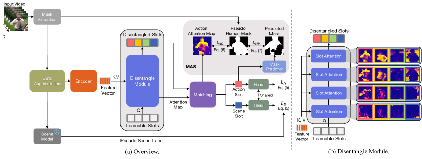
Figure 2: Overview of DEVIAS. (a) DEVIAS begins with augmenting an input video to diversify action-scene combinations in the training data. We extract pseudo-human masks of input videos in a minibatch to swap the scenes of the videos. Then we extract video features with an encoder using the scene-augmented video as an input. The disentangle module takes the feature vectors as keys and values for attention with learnable slots as queries and outputs disentangled slots. A matching function assigns each slot an action or a scene slot. We train action slots with ground-truth action labels and scene slots with pseudo-ground-truth soft scene labels predicted by a frozen scene model. To further guide action slot learning, we introduce MAS, leveraging pseudo-human masks. (b) Given input learnable slots as queries, the disentangle module iteratively attends to encoded features as keys and values. As a result of the iterative slot attention, the slots progressively learn distinct information, i.e. action, and scene, as shown in the attention map.

Disentangled representation learning.

Generative modeling works have extensively explored disentangled representation learning to manipulate each attribute for image/video generation [40, 10, 32, 6, 17, 50, 68, 55, 70, 33, 41, 78]. Disentangled representation learning for video understanding includes disentangling different attributes [65, 82], learning dynamic and static components of videos [66, 83], and disentangling action and scene [71, 45] to improve action recognition. We also focus on disentangled representations for video understanding. Unlike prior works that overlook the quality and utility of the scene representations [71, 45], we aim to learn not only high-quality action but also high-quality scene representations to achieve more holistic video understanding.

Mitigating scene bias in action recognition.

The community has identified scene bias [43, 11] as the devil of action recognition as biased models do not generalize well to new tasks/domains. Addressing scene bias has proven beneficial, enhancing performance in downstream tasks [11, 3, 67, 19], data efficiency [87, 27], and domain adaptation [12, 58]. Yet, an often-overlooked aspect is that action representations, when debiased from the scene context, may lose valuable contextual information. In contrast to scene-debiasing, DEVIAS learns disentangled action and scene representations. The disentangled representations are beneficial for both in-context and out-of-context video understanding.

3 DEVIAS

We introduce DEVIAS, a method for learning disentangled action and scene representations using a single model as illustrated in Figure 2. We augment an input video to obtain diverse action-scene combinations. Please refer to Appendix A for the details. In a minibatch, $\mathbf{I}\in\mathbb{R}^{B\times 2T\times H\times W\times C}$, consisting of $B$ videos of $2T$ frames, $H\times W$ spatial dimensions, and $C$ channels, we swap the scenes among the videos using extracted pseudo-human masks to get scene-augmented videos $\tilde{\mathbf{I}}$ with the same dimensions as $\mathbf{I}$. A feature encoder then extracts feature vectors $\mathbf{X}\in\mathbb{R}^{B\times NT\times D}$ of the scene-augmented videos $\tilde{\mathbf{I}}$, where $N$ is the number of spatial patches and $D$ is the dimension of patch embeddings. To capture distinct information from the feature vectors, i.e. action and scene, we introduce the disentangle module. The disentangle module takes the feature vectors as keys and values for attention with learnable slots as queries and outputs disentangled slots. A matching function categorizes each slot as either action or scene. We supervise action slot learning using ground-truth action labels covering $N_{A}$ action types and scene slot learning using scene labels covering $N_{S}$ scene types. We use a shared head for action and scene prediction. To further guide action slot learning, we introduce Mask-guided Action Slot learning (MAS), leveraging pseudo-human masks. We provide detailed descriptions of the disentangle module in Section 3.1, MAS in Section 3.2, and training & inference of DEVIAS in Section 3.3.

3.1 Disentangle Module

Slot attention for action scene disentanglement.

To learn disentangled action and scene representations, we build the disentangle module upon slot attention [46, 37]. In each slot attention iteration, we project input feature vectors $\mathbf{X}\in\mathbb{R}^{NT\times D}$, and $K$ learnable slots $\mathbf{S}\in\mathbb{R}^{K\times D}$ to a common space with the dimension $D_{h}$ as follows: $\mathbf{Q}=\mathbf{S}\mathbf{W}_{Q}\in\mathbb{R}^{K\times D_{h}}$, $\mathbf{K}=\mathbf{X}\mathbf{W}_{K}\in\mathbb{R}^{NT\times D_{h}}$, and $\mathbf{V}=\mathbf{X}\mathbf{W}_{V}\in\mathbb{R}^{NT\times D_{h}}$, where $\mathbf{W}_{Q}$, $\mathbf{W}_{K}$, and $\mathbf{W}_{V}$ are the $D\times D_{h}$ query, key, and value projection matrices, respectively. Here, we omit the batch dimension $B$, layer normalization [2], and GELU [30] for brevity. Comprehensive details are in Appendix A.

Given the query, key, and value, we define slot attention operation as follows:

$$\mathbf{M} =\mathbf{K}\mathbf{Q}^{\top}/\sqrt{D_{h}}.$$ (1)

Then we normalize the $NT\times K$ attention map $\mathbf{M}$ along the slot-axis instead of the key-axis using the softmax function, fostering competitive learning of action and scene representations in slots.

$$\mathbf{A}(n,k) =\frac{\exp{(\mathbf{M}(n,k)})}{\sum_{i=1}^{K}\exp{(\mathbf{M}(n,i))}}.$$ (2)

Here, $n$ is the key index and $k$ is the slot index. Then we normalize $\mathbf{A}$ along the key-axis using the $L^{2}$ norm function, yielding $\hat{\mathbf{A}}$. Then we attend to input features with the attention map $\hat{\mathbf{A}}$ as follows:

$$\mathbf{Z}=\hat{\mathbf{A}}^{\top}\mathbf{V}.$$ (3)

For each iteration $m\in[1,M]$, we update the slots by adding them to the slot attended feature maps $Z$ and pass the result through an MLP with a residual connection as follows:

$$\mathbf{S} =\texttt{MLP}(\mathbf{S}+\mathbf{Z})+\mathbf{S}+\mathbf{Z}.$$ (4)

The slots progressively encode disentangled action and scene information with iterative updates.

Matching.

We categorize each slot as an action or scene by solving a bipartite matching problem. We use the cross-entropy between a true label (or a pseudo label) and a prediction as the cost function for matching. We generate class predictions using a classification head $\psi$, shared across the action and scene tasks, as shown in Figure 2 (a). After computing a $K\times 2$ cost matrix, we solve the matching problem using the Hungarian algorithm [39].

Disentangle loss.

For action and scene slot learning, we define the disentangle loss with a unified head for predicting a $N_{A}+N_{S}$ dimensional vector as follows:

$$L_{D} =-\sum_{c=1}^{N_{A}+N_{S}}[y^{a}_{c}\log(\psi(\mathbf{S}_{action}))+y^{s}_{c}\log{\psi(\mathbf{S}_{scene})}].$$ (5)

Here, $\mathbf{y}^{a}$ denotes the ground-truth action label and $\mathbf{y}^{s}$ represents the soft scene label. $\mathbf{S}_{action}$ is the action slot, and $\mathbf{S}_{scene}$ is the scene slot. Scene action datasets often do not provide ground truth scene labels, we obtain $\mathbf{y}^{s}$ from a frozen off-the-shelf scene recognition model. For more details, please see Appendix A.

3.2 Mask-guided Action Slot learning

Since slots are in competition with each other, additional supervision for the action slot could be beneficial for the overall disentanglement of the slots. We introduce Mask-guided Action Slot learning (MAS) as shown in Figure 2. MAS takes the action slots $\mathbf{S}_{action}$, the keys $\mathbf{K}$, and the pseudo-human mask $\hat{\mathbf{H}}$ estimated through an off-the-shelf method [76, 14, 75, 19] as input. MAS consists of two auxiliary tasks: i) attention guidance, and ii) mask prediction.

Attention guidance.

In the attention guidance task, we encourage the attention map, $\mathbf{A}^{(M)}(:,k_{action})$, between the action slot $\mathbf{S}_{action}$ and the key $\mathbf{K}^{(M)}$ to resemble human masks, where $k_{action}$ is the action slot index selected by the Hungarian matching. To achieve this goal, we leverage pseudo-ground-truth human masks $\hat{\mathbf{H}}$ to supervise the action slot learning. We define the attention guidance loss as follows:

$$L_{AG} =||\mathbf{A}^{(M)}(:,k_{action})-\hat{\mathbf{H}}||_{2}^{2}.$$ (6)

Mask prediction.

In our mask prediction task, we employ a shallow MLP, denoted as $\phi$. The MLP takes the action slot as input to directly predict human masks. We opt for video-level human mask prediction over frame-level, as we empirically find it works well. We define the mask prediction loss as follows:

$$L_{MP}=-\tilde{\mathbf{H}}\log(\phi(\mathbf{S}_{action}))-(1-\tilde{\mathbf{H}})\log(1-\phi(\mathbf{S}_{action})).$$ (7)

Here, $\tilde{\mathbf{H}}\in\mathbb{R}^{N}$ represents the temporally averaged version of the pseudo-ground-truth human masks $\hat{\mathbf{H}}\in\mathbb{R}^{NT}$.

3.3 Training and Inference

Training.

For model training, we define a total loss function as follows:

$$L=L_{D}+\alpha L_{MD}+\beta L_{MP}+\gamma L_{cos}.$$ (8)

Here, we incorporate the cosine similarity loss between every pair of slots, $L_{cos}$, to diversify slots. $\alpha$, $\beta$, and $\gamma$ are hyperparameters to adjust the contribution of each loss term.

Inference.

During the inference, we omit the data augmentation, the frozen scene model, and the MAS module. We input a video into the model to extract $K$ slots. Among the $K$ slots, we assign action and scene slots based on the highest output probability. The linear classifier $\psi$ takes the action and scene slots to predict the action and scene labels.

4 Experimental Results

In this section, we demonstrate extensive experimental results to answer the following questions: (1) Are the learned representations disentangled? (Section 4.5) (2) Are the disentangled representations effective? (Section 4.6) (3) Does DEVIAS outperform the baselines in achieving a balanced learning of action and scene representations in both in-context and out-of-context scenarios? (Section 4.6) (4) How can we effectively disentangle action and scene representations? (Section 4.8) To this end, we first provide details about the implementations in Section 4.1, the datasets in Section 4.2, the evaluation metric in Section 4.3, and the baselines in Section 4.4.

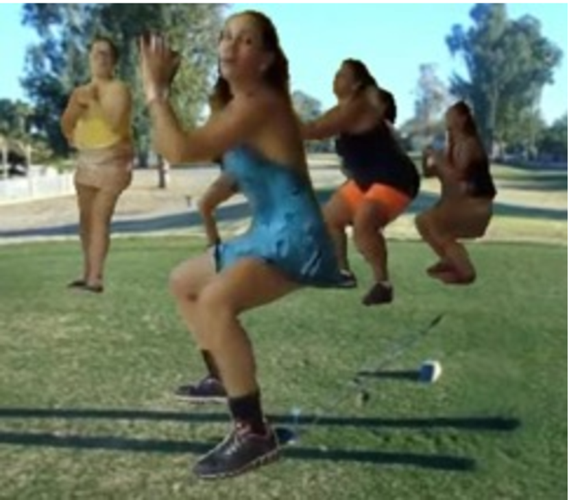
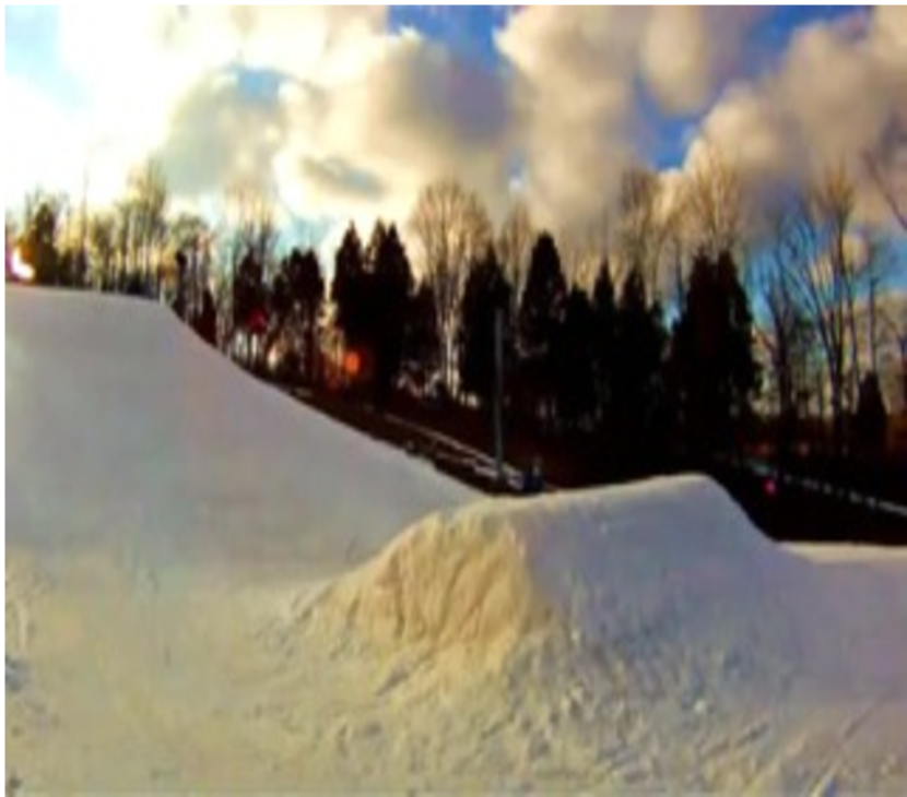
(a)

(b)

(c)

Figure 3: Example frames of the out-of-context datasets. (a) playing basketball in a lake from SCUBA Places365 [42], (b) dancing on a golf coarse from HAT Far [13], and (c) snowfield from HAT Scene-Only [13].

4.1 Implementation Details

In this section, we briefly explain the implementation details. For the comprehensive details, please refer to Appendix B.

Training

We densely sample 16 frames from each video to construct an input clip. We apply random cropping and resizing to every frame to get $224\times 224$ pixels for each frame. We employ the ViT [21] pre-trained with self-supervised VideoMAE [62] on the target dataset e.g. UCF101, and Kinetics-400 as the feature encoder. We use FAME [19] for the pseudo-human-mask extraction. We employ the ViT pre-trained on the Places365 [86] dataset as the frozen scene model.

Inference

During inference, we average predictions over multiple temporal views and spatial crops, employing 2$\times$3 views in all experiments.

Table 1: Sanity check on action-scene disentanglement using K-NN. We compare models trained on the UCF-101 [60] dataset using K-NN classification accuracy (%) on the UCF-101 and HMDB-51 [38] datasets. For each column, we show {train}-{test} features of K-NN. ‘A’ represents action, and ‘S’ indicates scene. The best performance is highlighted.

Method	K-NN Normal Features (↑)						K-NN Reverse Features (↓)
	UCF-101			HMDB-51			UCF-101			HMDB-51
	A-A	S-S		A-A	S-S		A-S	S-A		A-S	S-A
Random	1.0	0.3		1.0	0.3		1.0	0.3		1.0	0.3
One-Token	87.7	43.5		43.4	27.5		87.7	43.5		43.4	27.5
Two-Token	84.2	43.6		37.4	25.7		62.8	37.1		27.3	20.7
DEVIAS	89.7	41.8		38.8	26.3		4.5	0.3		1.9	0.9
Upperbound	92.0	48.8		60.5	38.1		-	-		-	-

4.2 Datasets

To validate the disentanglement, we use the train splits of UCF-101 [60] and Kinetics-400 [36] for model training. For testing, we use not only the in-context datasets i.e. as UCF-101 and Kinetics-400 validation splits but also the out-of-context datasets i.e. SCUBA [42] and HAT [13]. SCUBA [42] comprises videos created by superimposing action regions from one video onto various scenes, including those from Places365 [86], VQGAN-CLIP [15] generated scenes and sinusoids. HAT [13] is a similar mixed-up dataset, but it provides multiple splits with distinct characteristics such as Scene-Only, and Random/Close/Far. ‘Scene-Only’ means humans are eliminated from a video using segmenting and inpainting techniques. ‘Random’ refers to a mix of actions and scenes in a completely arbitrary manner. ‘Close’ denotes the combination of actions and scenes from within the same action category. In contrast, ‘Far’ indicates the mixing of actions and scenes from different categories. We show example frames of each dataset in Figure 3. For more details, please refer to Appendix D.

Table 2: Action and scene recognition performance on the UCF-101 dataset. We report the Top-1 action recognition accuracy (%) and the Top-5 scene recognition accuracy (%). We evaluate both in-context and out-of-context recognition performances. We also report the harmonic mean (H.M.) of the action recognition and scene recognition. The best and the second-best H.M. numbers are highlighted. $\dagger$ indicates that we use a linear probe evaluation for the task for which direct supervision is not provided.

Supervision	Training Strategy	Method	Action($\uparrow$)					Scene($\uparrow$)
			In-Context	Out-of-Context (SCUBA [42])					In-Context	Out-of-Context (HAT [13])				H.M.
				Places365	VQGAN-CLIP	Sinusoid	Mean			Scene-Only	Random	Far	Mean
Action$\dagger$	Naive	Action ViT	92.9	15.0	12.4	21.0	16.1		62.9	50.2	49.9	56.6	52.2	37.1
		Action ViT w/ Aug.	90.0	19.1	18.8	19.4	19.1		64.0	52.0	54.0	63.3	56.4	41.3
	Scene Debiasing	BE [67]	92.3	16.1	12.1	38.7	22.3		63.6	51.7	52.6	59.4	54.6	44.6
		FAME [19]	91.6	22.0	24.8	15.6	20.8		62.7	51.2	48.7	54.5	51.5	42.4
Scene$\dagger$	Naive	Scene ViT	69.2	2.2	0.9	7.1	3.4		72.0	61.7	62.8	69.6	64.7	11.8
	Multi-Task	One-Token	91.9	10.5	5.0	21.8	12.4		74.0	60.5	58.0	66.5	61.7	33.0
Action	Disentangle	Two-Token	86.0	11.9	11.1	19.9	14.3		72.3	59.6	59.2	67.1	62.0	35.9
&		Two-Token w/ BE [67]	89.9	15.0	13.0	20.5	16.2		74.2	62.3	59.3	69.5	63.7	39.2
Scene		Two-Token w/ FAME [19]	89.5	21.7	25.3	15.3	20.7		73.2	61.4	62.8	70.3	64.8	45.2
		DEVIAS	90.1	41.1	40.1	38.6	40.0		74.0	61.0	62.4	70.2	64.5	61.4

4.3 Evaluation Metric

To evaluate methods, we report action and scene recognition performance across both in-context and out-of-context datasets. We use top-1 accuracy as the metric for action recognition. In the case of scene recognition, we rely on pseudo-labels generated by a scene model pre-trained on Places365 [86], as most video datasets lack comprehensive action or scene labels. Given the fine-grained nature of the Places365 categories, we choose top-5 accuracy as the metric for scene recognition. To gauge a model’s balanced understanding of both in-context and out-of-context scenarios, we use the harmonic mean (H.M.) across four performance metrics as our main metric: i) in-context action, ii) out-of-context action, iii) in-context scene, and iv) out-of-context scene.

4.4 Baselines

We compare DEVIAS with several baselines, including two ViT models trained solely using action or scene labels. Additionally, we consider scene-debiasing baselines such BE [67] and FAME [19] trained only with action labels. For methods trained with single-type supervision, we use a linear probe evaluation for the task for which direct supervision is not provided.

DEVIAS extends from a simple baseline, the Two-Token approach. The Two-Token baseline involves a feature encoder and two distinct learnable tokens: one for action and another for scene, appended to the input patches. We supervise the action token learning with the ground truth action label and the scene token learning with the soft pseudo-scene label. Additionally, we explore two variations of this baseline, each incorporating either the BE [67] or FAME [19] debiasing strategy.

Another baseline is the One-Token baseline. Unlike the Two-Token approach, this baseline has a single token and employs a multi-task loss combining both action and scene losses to train this singular token. For more details, please see Appendix C.

4.5 Sanity-Check: K-NN Experiments

Prior to the main experiments, we conduct a sanity check on DEVIAS. For representation learning, we train DEVIAS and the baselines on the UCF-101 [60] train split. Then we extract and store the action and scene feature vectors from all the training videos in the target datasets, UCF-101 and HMDB-51 [38]. For K-NN testing, we evaluate performance in two scenarios: using the same feature types as in training (denoted as K-NN Normal Features), and using the alternate feature types (referred to as K-NN Reverse Features). e.g. ‘A-S’ indicates training the K-NN classifier with action features and testing with scene features. We anticipate that if a model has disentangled action and scene representations, it would perform well in the K-NN Normal Features scenario, and show near-random performance in the K-NN Reverse Features scenario.

In Table 1, we compare our method with the One-Token and Two-Token baselines and the random performance. For the experiments, we employ a 10-NN setting and report top-1 accuracy. We train both the baseline and DEVIAS on UCF-101, and the upper bound represents the performance achieved with supervised training on each dataset. In the K-NN Normal Features scenario, all the methods compared show reasonable action and scene recognition performances. However, in the K-NN Reverse scenario, only DEVIAS shows near-random performance. The results verify the disentangled action and scene representations of DEVIAS.

Table 3: Action and scene recognition performance on the Kinetics-400 dataset. We report the Top-1 action recognition accuracy (%) and the Top-5 scene recognition accuracy (%). We evaluate both in-context and out-of-context recognition performances. We also report the harmonic mean (H.M.) of the action recognition and scene recognition. The best and the second-best H.M. numbers are highlighted. $\dagger$ indicates that we use a linear probe evaluation for the task for which direct supervision is not provided.

Supervision	Training Strategy	Method	Action($\uparrow$)					Scene($\uparrow$)
			In-Context	Out-of-Context (SCUBA [42])					In-Context	Out-of-Context (HAT [13])				H.M.
				Places365	VQGAN-CLIP	Sinusoid	Mean			Scene-Only	Random	Far	Mean
Action$\dagger$	Naive	Action ViT	76.8	42.3	43.5	49.9	45.2		71.2	65.8	63.0	66.2	65.0	61.9
		Action ViT w/ Aug.	77.6	50.7	49.4	57.3	52.5		71.6	65.7	63.7	66.3	65.2	65.3
	Scene Debiasing	BE [67]	77.6	44.3	44.3	52.0	46.9		70.7	65.4	63.0	65.0	64.5	62.6
		FAME [19]	77.8	50.0	50.8	57.0	52.6		70.3	64.9	61.0	63.4	63.1	64.6
Scene$\dagger$	Naive	Scene ViT	43.0	9.8	8.0	15.8	11.2		86.5	82.6	79.9	81.2	81.2	29.3
	Multi-Task	One-Token	74.2	35.3	36.4	46.2	39.3		87.9	83.8	80.8	81.5	82.0	64.0
Action	Disentangle	Two-Token	75.1	37.1	36.4	47.2	40.2		86.4	75.8	78.3	80.3	78.1	63.9
&		Two-Token w/ BE [67]	75.1	37.4	37.3	48.0	40.9		87.7	82.9	80.0	81.5	81.5	65.1
Scene		Two-Token w/ FAME [19]	75.0	35.8	37.6	52.1	41.8		87.3	77.4	81.1	82.6	80.4	65.4
		DEVIAS	77.3	51.8	53.0	59.7	54.8		82.0	76.5	75.7	77.1	76.4	70.8

4.6 Quantitative Analysis

We validate the performance of DEVIAS through extensive experiments. In Table 2, we evaluate the methods on the UCF-101 dataset. The models trained solely under action supervision show significant performance drops in out-of-context scenarios. For instance, the baseline Action ViT shows more than $75$ points accuracy drop. Applying scene debiasing [67, 19] improves the out-of-context action performance. However, the scene debiasing models show inferior scene recognition performance compared to the baseline Scene ViT trained with scene supervision only: e.g. FAME $51.5\%$ vs. the naive Scene ViT $64.7\%$ in out-of-context scene recognition.

The action performance of the Two-Token baseline decreases compared to the Action ViT baseline in both in-context and out-of-context scenarios, dropping from $92.9\%$ to $86.0\%$, and from $16.1\%$ to $14.3\%$, respectively. The results indicate that the Two-Token baseline still learns scene-biased representations. When we apply scene debiasing to the Two-Token baseline, we observe some improvement of $1.9\sim 6.4$ points in out-of-context action performance and $3.3\sim 9.3$ points improvement in harmonic mean compared to the Two-Token without debiasing, suggesting an enhanced balance in performance compared to the Two-Token baseline without debiasing.

DEVIAS stands out by showing a more balanced understanding of action and scene, achieving a significant $16.2$ points boost over the second-best method in the Harmonic Mean(H.M.). Particularly in out-of-context action scenarios, DEVIAS outperforms the second-best method by $17.7$ points, showcasing its robustness in action recognition regardless of the surrounding context. Remarkably, DEVIAS as a singular model surpasses the combined harmonic mean of the best individual in-context and out-of-context action and scene performances ($61.4\%$ vs. $47.0\%$), indicating effective and efficient disentanglement of representations.

In Table 3, we present the experimental results on the Kinetics-400 dataset, where DEVIAS shows a $5.4$ points improvement in harmonic mean over the second-best method. The overall trend among methods remains similar to the trend we observe in the UCF-101 dataset.

4.7 Qualitative Analysis

To gain deeper insights, we carry out two qualitative analyses. We first show the slot attention map in Figure 4. In both in-context and out-of-context scenarios, each slot attends to action and scene regions well. We also show UMAP [51] visualization of the feature vectors of the baselines, Two-Token, Two-Token w/ BE, and Two-Token w/ FAME, and DEVIAS as shown in Figure 5. Compared to the baselines, DEVIAS clearly demonstrates a distinct separation between action and scene feature vectors.

Input Frame

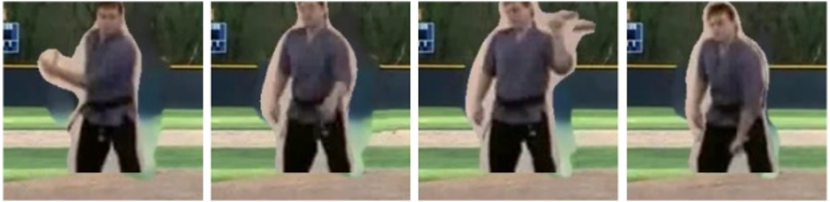
Action Slot

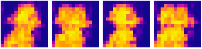
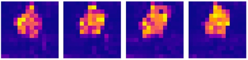
Scene Slot

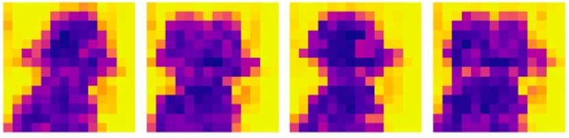
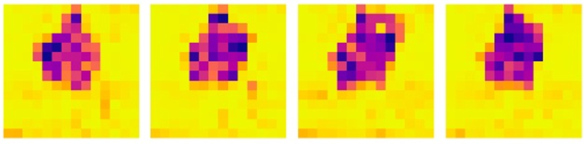
(a) In-Context

(b) Out-of-Context

Figure 4: Visualization of DEVIAS slot attention map. (a) In-Context video from UCF-101 [60], (b) Out-of-Context video from HAT Far [13]. Each slot attends to action and scene regions well across frames regardless of in-context or out-of-context.

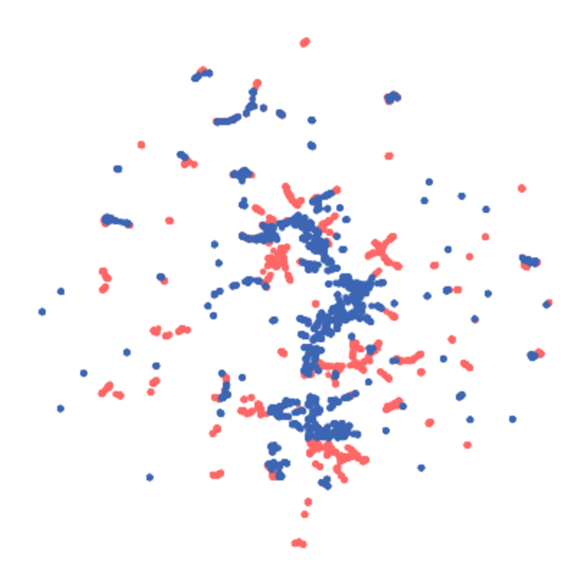
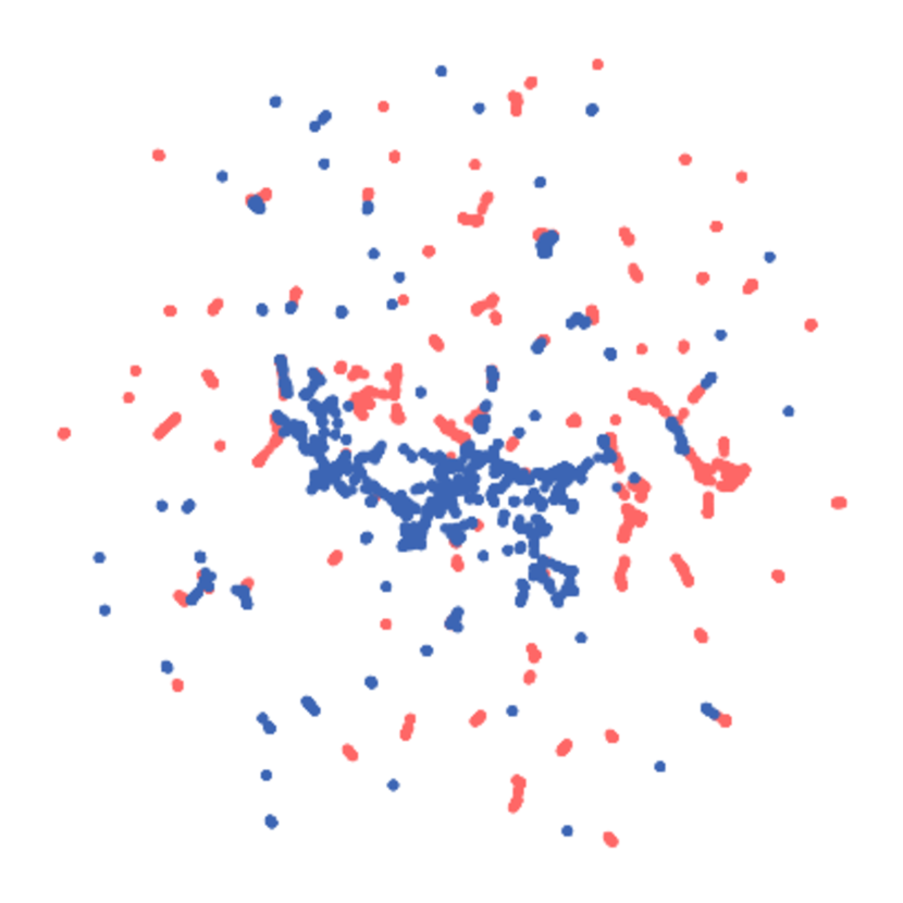
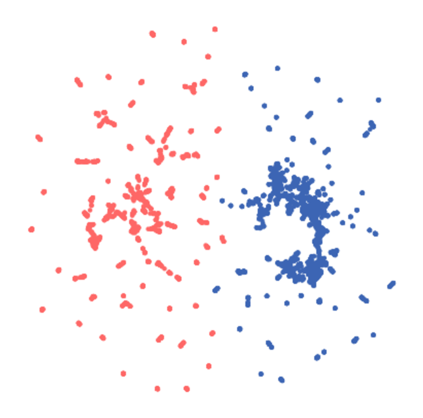
(a) Two-Token

(b) Two-Token w/ BE [67]

(c) Two-Token w/ FAME [19]

(d) DEVIAS

Figure 5: UMAP [51] visualization of feature vectors on UCF-101 dataset, test split. (a) Two-Token, (b) Two-Token w/ BE, and (c) Two-Token w/ FAME baselines show entangled action and scene feature vectors. In contrast, (c) our DEVIAS demonstrates a distinct separation between action and scene feature vectors. All models are trained on the UCF-101 train split. Best viewed with zoom and color.

4.8 Ablation Study

We conduct extensive ablation studies to validate the effectiveness of each proposed module and design choices. Here, we conduct all experiments on the UCF-101 [60] dataset. For evaluating action performance, we report top-1 accuracy on the in-context UCF-101, and out-of-context SCUBA-UCF-101-Places [42]. For scene performance, we report top-5 accuracy on the in-context UCF-101 and out-of-context UCF-101-Scene-only [13]. We report the harmonic mean (H.M.) of the four performances to assess the balanced performance of action and scene.

Table 4: Ablation study. To validate the effect of each component, we show the results on the UCF-101 dataset. In every experiment, we use a ViT backbone pre-trained on the UCF-101. We report the Top-1 accuracy (%) for the action recognition and the Top-5 accuracy (%) for the scene recognition, along with the harmonic mean (H.M.) of the two accuracies. The best numbers are highlighted.

(a) Effect of disentangle module.

(b) Effect of mask-guided action slot learning.

Method	Action($\uparrow$)		Scene($\uparrow$)		H.M.
	In-Context	SCUBA-Places	In-Context	Scene-Only
w/o disentangle module	89.5	21.7	73.2	61.4	45.9
w/ disentangle module	90.0	31.9	73.7	59.8	55.0

Method		Action($\uparrow$)		Scene($\uparrow$)		H.M.
Attn. Guidance	Mask Pred.	In-Context	SCUBA-Places	In-Context	Scene-Only
$\times$	$\times$	90.0	31.9	73.7	59.8	55.0
$\times$	✓	89.7	33.6	73.4	60.5	56.3
✓	$\times$	90.8	40.6	73.8	59.8	60.7
✓	✓	90.1	41.1	74.0	61.0	61.2

(c) Effect of slot assignment method.

(d) Effect of softmax normalization axis.

Method	Action($\uparrow$)		Scene($\uparrow$)		H.M.
	In-Context	SCUBA-Places	In-Context	Scene-Only
Hard assign	89.4	33.8	71.1	58.3	55.6
Hungarian	90.1	41.1	74.0	61.0	61.2

Axis	Action($\uparrow$)		Scene($\uparrow$)		H.M.
	In-Context	SCUBA-Places	In-Context	Scene-Only
Keys	89.6	32.4	73.9	61.6	55.7
Slots	90.1	41.1	74.0	61.0	61.2

(e) Effect of mask extraction method.

(f) Effect of hyperparameters.

Method	Action($\uparrow$)		Scene($\uparrow$)		H.M.
	In-Context	SCUBA-Places	In-Context	Scene-Only
FAME [19]	90.1	41.1	74.0	61.0	61.2
Segformer [76]	90.0	45.3	73.8	59.9	63.1

Hyperparameters			Action($\uparrow$)		Scene($\uparrow$)		H.M.
No. Slots	No. Iter.	Shared?	In-Context	SCUBA-Places	In-Context	Scene-Only
2	2	✓	90.5	37.2	73.5	59.4	58.5
2	4	✓	90.1	41.1	74.0	61.0	61.2
2	4	$\times$	89.1	34.2	70.7	57.7	55.7
4	4	✓	89.1	39.2	71.3	58.6	59.0

Effect of the disentangle module.

We investigate the effect of the disentangle module. We compare DEVIAS without MAS to the Two-Token baseline w/ FAME debiasing baseline. As shown in Table 4 (a), incorporating the disentangle module results in $9.1$ points enhancement in the harmonic mean compared to the baseline.

Effect of MAS.

In Table 4 (b), we investigate the effect of MAS. When using both auxiliary tasks, we observe an increase of $6.2$ points in the harmonic mean compared to the baseline without any auxiliary tasks.

Effect of slot assignment method.

We examine the Hungarian matching when assigning disentangled slots as action or scene slots and present the results in Table 4 (c). We observe a $5.6$ points improvement in harmonic mean when training with the Hungarian matching, compared to a fixed assignment of each slot to action and scene roles.

Effect of softmax normalization axis.

In Table 4 (d), we analyze the effect of the softmax normalization axis. Applying softmax normalization along the slot-axis, as opposed to the conventional key-axis normalization, results in a gain of $5.5$ points in the harmonic mean. The results indicate that slot attention, by competitively isolating features, significantly contributes to disentangled representation learning.

Effect of mask extraction method.

Throughout our experiments, we utilize a simple mask extraction approach without learning [19] by default. However, when using a learned segmentation method e.g. SegFormer [76], we observe a further improvement: $1.9$ points increase in harmonic mean as shown in Table 4 (e).

Effect of hyperparameters.

Observing the first and second rows in Table 4 (f), we see that increasing the number of iterations in the disentangle module improves the harmonic mean by $2.7$ points. Using shared parameters for slot attention shows $5.5$ points improvement to using separate parameters for slot attention. We see a decrease in performance when using more slots, as shown in the fourth row.

5 Conclusions

In this paper, we tackle the problem of disentangled action and scene representation learning for holistic video understanding. We introduce DEVIAS, a method that employs slot attention and mask-guided action slot learning to disentangle action and scene representations. Through rigorous experiments, we assess DEVIAS across various contexts, both in-context and out-of-context, considering both action and scene performance metrics. The results showcase the effectiveness of the DEVIAS in learning disentangled action and scene representations as a single model.

Appendix

In this Appendix, we provide comprehensive method/im-plementation/baseline/dataset details, quantitative/quali-tative results, and downstream task performance to complement the main paper. We organize the Appendix as follows:

1. Additional Details about DEVIAS

2. Complete implementation details

3. Compared method details

4. Dataset details

5. Additional results

6. Downstream task performance

Appendix A Additional Details about DEVIAS

In this section, we provide details of DEVIAS. In our implementation, we employ ViT-Base [21] as the encoder.

Data augmentation.

In DEVIAS, we augment input videos to diversify action-scene combinations. Previous works [87, 19] have demonstrated that scene augmentation by mixing up using a human mask improves action recognition. We mix a video $\mathbf{V}_{i}$ with another video $\mathbf{V}_{j}$ within a minibatch, by cut-and-paste operation as follows:

$$\tilde{\mathbf{V}}_{i}=\mathbf{V}_{i}\odot\tilde{\mathbf{H}}_{i}+\mathbf{V}_{j}\odot(1-\tilde{\mathbf{H}}_{i}),$$ (9)

where , $\tilde{\mathbf{H}}_{i}$ is a pseudo-human mask of the video $\mathbf{V}_{i}$ extracted by an off-the-shelf method [19]. This simple scenario augmentation can diversify action-scene combinations in a training dataset.

Scene model.

Most action datasets do not provide ground-truth scene labels. Consequently, we opt to use a ViT-Base as a frozen scene model to generate pseudo scene labels for each video in the action datasets we use. We prepare the frozen scene model by training a ViT-Base on the Places365 [86] dataset. Given that we are dealing with video data, we inflate the static images of the Places365 dataset to introduce a temporal dimension. We generate a pseudo scene label, denoted as $y^{s}$, by taking the frozen scene model prediction on a video $\mathbf{V}$.

Unified classification head.

We employ a unified linear classification head, $\psi$, designed to output a vector of dimension $N_{A}+N_{S}$, for predicting both action with $N_{A}$ classes and scene with $N_{S}$ classes.

Slot matching.

Following the previous works [46, 7], we employ the Hungarian algorithm [39] as our matching function to assign each learned slot as either an action or scene based on the matching cost. We use the cross-entropy between a true label (or a pseudo label) and a prediction as the cost function for matching. In order to align the dimensions of the (pseudo) ground-truth label with those of the unified head, we zero-pad the end of the (pseudo) ground-truth label, extending it to match the combined length of $N_{A}+N_{S}$.

Disentangle module.

Algorithm 1 Disentangle Module

1:  INPUT: Slots $\mathbf{S}\in\mathbb{R}^{K\times D}$, Features $\mathbf{X}\in\mathbb{R}^{NT\times D}$, Number of iterations $M$, and Hidden dimension $D_{h}$

2:  Layer params: $\mathbf{W}_{Q}$, $\mathbf{W}_{K}$, $\mathbf{W}_{V}$: $\mathbb{R}^{D\times D_{h}}$ linear projections for attention; LayerNorm; Linear, GELU for MLP

3:  for $m=1$ to $M$ do

4:     $\mathbf{Q}=\mathbf{W}_{Q}(\text{LayerNorm}(\mathbf{S}))$

5:     $\mathbf{K}=\mathbf{W}_{K}(\text{LayerNorm}(\mathbf{X}))$

6:     $\mathbf{V}=\mathbf{W}_{V}(\text{LayerNorm}(\mathbf{X}))$

7:     $\mathbf{A}=\text{Softmax}\left(\frac{\mathbf{K}\mathbf{Q}^{\top}}{\sqrt{D_{h}}},\text{axis=`slots'}\right)$

8:     $\hat{\mathbf{A}}$ = L2Norm($\mathbf{A},\text{axis=`key'}$)

9:     $\mathbf{Z}=\hat{\mathbf{A}}^{\top}\mathbf{V}$

10:     $\mathbf{Z}_{\text{mlp}}=\text{Linear}(\text{GELU}(\text{Linear}(\mathbf{S}+\mathbf{Z})))$

11:     $\mathbf{S}=\mathbf{Z}_{\text{mlp}}+\mathbf{S}+\mathbf{Z}$

12:  end for

13:  return  $\mathbf{S}$

We provide a detailed pseudo-code for the disentangle module in Algorithm 1. Note that within the disentangle module, all linear layers share weights.

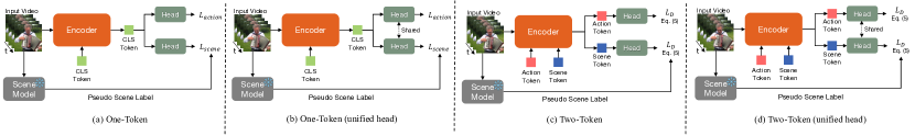
Figure 6: Architecture visualization of baselines. All baselines use the same encoder, ViT [21]. (a) and (b) use a single token, and (c) and (d) use separate tokens for action and scene. (a) and (c) use separate classification heads for action and scene, and (b) and (d) use a unified classification head. Best viewed with zoom and color.

Appendix B Complete Implementation Details

In this section, we provide comprehensive details of our experimental setup and implementation details. We conduct the experiments with 24 NVIDIA GeForce RTX 3090 GPUs. We build upon the codebase of VideoMAE [62]. We implement DEVIAS using the DeepSpeed frameworks for faster training.

Data preprocessing.

We densely sample frames from a video to obtain a clip of 3 channels $\times$ 16 frames $\times$ 224 width $\times$ 224 height. We set the frame interval as 4 frames for the dense sampling. Given the sampled clip, we apply the data augmentation described in (9). We use the augmented clip as an input to the encoder and the scene model. Following VideoMAE [62], we employ 3D convolution for patch embedding to effectively reduce the temporal dimension by half. This process results in a total of 8 $\times$ 196 tokens. We maintain this data preprocessing protocol consistent across all experiments.

Scene model training.

We employ a ViT-Base, pre-trained on the ImageNet-1k [16] with the MAE [29] training method, fine-tuned on the Places365 [86] as the scene model. Given that we are dealing with video data, we inflate the static images of the Places365 dataset to introduce a temporal dimension. We summarize the hyperparameters used in Table 9.

Model training.

We employ ViT-Base as our encoder. We use ViT-Base pre-trained with VideoMAE [62] training on the dataset we use in the main paper, e.g. UCF-101 and Kinetics-400. In the case of the UCF-101, we further fine-tune the pre-trained ViT-Base with action supervision, before the disentangled representation learning as we empirically find it is beneficial for stabilizing the training process. We obtain the pseudo-human mask for both UCF-101 and Kinetics-400 datasets using FAME [19] as it does not require any external object detector. FAME extracts the moving foreground region from the background regions using frame difference and color statistics. In FAME, the parameter $\tau$ represents the threshold for the foreground ratio in the mask, selecting the top-k percentage as the foreground. For instance, a $\tau$ value of 0.4 indicates that the top 40% of the mask is considered as foreground regions. The augmentation ratio within a batch, denoted by $\rho$, determines the proportion of scene augmented data in a batch using (9). For UCF-101, we set $\tau$ and $\rho$ to 0.3 and 0.4, respectively, while for Kinetics-400, we set them to 0.5 and 0.8. We linearly scale the base learning rate, then $\text{\emph{actual lr}}=\text{\emph{base lr}}\times\text{\emph{Per GPU batch size}}\times\text{\emph{number of GPUs}}/256$. We summarize the hyperparameters used in Table 17.

Linear probe.

We use the linear probe evaluation protocol for the task for which direct supervision is not provided. For instance, after training a model with action supervision only, we evaluate the scene performance using the linear probe protocol. Similarly, when we train a model with scene supervision, we apply the linear probe protocol to evaluate the action performance. For the scene and action linear probe evaluation, we use the same hyperparameters. We summarize the hyperparameters used for each dataset in Table 12.

Inference.

During inference, we sample an input video multiple times to generate multiple temporal views. We resize each frame of each temporal view to $256\times 256$. Subsequently, we crop the video multiple times to generate multiple spatial crops. The final prediction is obtained by aggregating predictions from (temporal views) $\times$ (spatial crops). For the both UCF-101 and Kinetics-400 datasets, we employ a configuration of (2 clips) $\times$ (3 crops) configuration.

Appendix C Compared Method Details

In this section, we provide detailed descriptions of the methods and baselines compared with DEVIAS in the experiments.

Naive baselines.

We define the baselines with single supervision, either action or scene, without considering debiasing and disentangling as naive baselines. We have three naive baselines: i) the naive baseline ViT with action supervision denoted as Action ViT, ii) the naive baseline ViT with action supervision and some data augmentations denoted as Action ViT w/ Aug., iii) the naive baseline ViT with scene supervision denoted as Scene ViT. All three baselines are equipped with ViT-Base as the backbone. We summarize the hyperparameters used in Table 13, Table 14 and Table 10. In the Action ViT w/ Aug. baselines, we employ mixup [81], cutmix [80], and random erasing [84] augmentations to add some robustness. The Scene ViT is exactly the same as the Action ViT except that we use pseudo-scene labels instead of action labels.

Scene debiasing methods.

We compare DEVIAS with state-of-the-art self-supervised scene debiasing methods: BE [67] and FAME [19]. We employ a ViT-Base as an encoder and use either BE or FAME as a scene-debiasing data augmentation. BE randomly selects a frame from the same video and mixes it with the other frames, using a weight drawn from a uniform distribution between 0 and 0.3. FAME extracts a foreground mask and shuffles the background regions among the videos as denoted in (9), with both $\tau$ and $\rho$ parameters set to 0.5. We summarize the hyperparameters used in Table 15 and Table 16.

Disentangling baselines.

We provide a detailed description and figures for the disentangling baselines. We show the One-Token baseline in Figure 6 (a). We train the one-token model with a single classification token from ViT [21]. The Two-Token baseline uses two distinct learnable tokens: one is for action and another is for the scene, as depicted in Figure 6 (c). Both the One-Token and Two-Token baselines have separate heads for action and scene classification. $L_{action}$ is the cross-entropy loss with the ground-truth action label and $L_{scene}$ is the cross-entropy with the pseudo-scene label.

For a more detailed ablation study, we replace the separate classification heads in Figure 6 (a) and (c) with a single unified classification head, as shown in Figure 6 (b) and (d). In models with a unified classification head, we use the disentangling loss, $L_{D}$, described in the main paper. The hyperparameter setting is identical to the setting for the Action ViT. We summarize the hyperparameters used in Table 13. Additionally, we add either the BE or FAME as a data augmentation on top of the disentangling baseline with separate classification heads (Figure 6 (c)). We summarize the hyperparameters used for these settings in Table 15 and Table 16.

Appendix D Dataset Details

In this section, we provide a detailed description of the datasets.

D.1 Training dataset

We train DEVIAS and baselines on the train set of the UCF-101 [60], and Kinetics-400 [36] datasets. The UCF-101 [60] dataset consists of 9,537 training videos and 3,783 test videos from 101 classes. The Kinetics-400 [36] dataset comprises $\sim$ 240K training videos and $\sim$20K validation videos from 400 classes.

D.2 Test dataset

For testing, we use the test or validation set of diverse datasets for thorough evaluation: UCF-101, Kinetics-400, HAT [13], and SCUBA [42]. Since all the datasets do not have ground-truth scene labels, we generate pseudo-scene labels using the scene model described in Section A. We categorize the datasets into in-context datasets and out-of-context datasets.

Table 5: Action and scene recognition performance on the UCF-101 dataset. We report the Top-1 action recognition accuracy and the Top-5 scene recognition accuracy. We evaluate both in-context and out-of-context recognition performances. We also report the harmonic mean (H.M.) of the action recognition and scene recognition. The best and the second-best H.M. numbers are highlighted. $\dagger$ indicates that we use a linear probe evaluation for the task for which direct supervision is not provided.

Supervision	Training Strategy	Method	Action($\uparrow$)									Scene($\uparrow$)
			In-Context	Out-of-Context									In-Context	Out-of-Context
				SCUBA [42]				HAT [13]			Mean			HAT [13]				Mean
				Places365	VQGAN-CLIP	Sinusoid		Random	Close	Far				Scene-Only	Random	Close	Far		H.M.
Action$\dagger$	Naive	Action ViT	92.9	15.0	12.4	21.0		23.5	27.7	14.1	19.0		62.9	50.2	49.9	50.8	56.6	51.9	40.6
		Action ViT w/ Aug.	90.0	19.1	18.8	19.4		21.4	27.3	13.0	19.8		64.0	52.0	54.0	51.9	63.3	55.3	42.0
	Scene Debiasing	BE [67]	92.3	16.1	12.1	38.7		29.6	34.5	19.2	25.0		63.6	51.7	52.6	52.1	59.4	54.0	47.0
		FAME [19]	91.6	22.0	24.8	15.6		36.7	41.7	30.6	28.6		62.7	51.2	48.7	50.8	54.5	51.3	49.2
Scene$\dagger$	Naive	Scene ViT	69.2	2.2	0.9	7.1		8.7	14.3	3.2	6.1		72.0	61.7	62.8	60.8	69.6	63.7	19.2
	Multi-Task	One-Token	91.9	10.5	5.0	21.8		19.8	27.9	8.8	15.6		74.0	60.5	58.0	57.6	66.5	60.7	38.1
Action	Disentangle	Two-Token	86.0	11.9	11.1	19.9		17.3	23.9	9.1	15.5		72.3	59.6	59.2	57.8	67.1	60.9	37.6
&		Two-Token w/ BE [67]	89.9	15.0	13.0	20.5		22.4	29.0	12.2	18.7		74.2	62.3	59.3	58.4	69.5	62.4	42.5
Scene		Two-Token w/ FAME [19]	89.5	21.7	25.3	15.3		32.9	38.2	26.4	26.6		73.2	61.4	62.8	61.3	70.3	64.0	51.2
		DEVIAS	90.1	41.1	40.1	38.6		39.4	41.3	35.2	39.3		74.0	61.0	62.4	59.8	70.2	63.4	60.8

In-context datasets.

In-context datasets consist of actions with frequent scene context, e.g. playing basketball on a basketball court. In action recognition, datasets such as UCF-101 [60], and Kinetics-400 [36] are considered as in-context datasets, exhibiting a high correlation between action and scene [43, 11]. We evaluate our model on the test set of the UCF-101 dataset (3,783 videos) and the validation set of the Kinetics-400 dataset ($\sim$ 20K videos) in this paper.

Out-of-context datasets.

Out-of-context datasets consist of actions occurring in an unexpected or less expected scene: e.g. dancing in the mall [11]. SCUBA [42] and HAT [13] synthesize out-of-context datasets by applying segmentation models to in-context datasets such as UCF-101 and Kinetics-400. Please note that both the SCUBA and HAT datasets do not provide a training set.

SCUBA [42] comprises videos created by superimposing action regions extracted from a video onto various scenes. There are three different scene sources: i) the validation set of Places365 [86], ii) 2000 scene images generated by VQGAN-CLIP [15] with the template of a random category of Places365 and a random artistic style, and iii) random images with S-shaped stripe patterns generated by sinusoidal functions. The UCF-101-SCUBA consists of combinations of 910 videos in the first split of the UCF-101 validation set and five randomly selected scene images from each source, resulting in a total of 4,550 videos for each source. Each set of the Kinetics-400-SCUBA, i.e. Kinetics-400-SCUBA-Places365, Kinetics-400-SCUBA-VQGAN-CLIP, and Kinetics-400-SCUBA-Sinusoid, contains 10,190 videos for each background source, generated by pairing 10,190 videos from the Kinetics-400 validation set with a single background image. There exists a version assessed by Amazon Mechanical Turk (AMT) human workers to determine whether the video clearly holds the action. Following the previous work [42], we use the version without AMT human assessment for a fair comparison.

HAT [13] is another synthesized dataset for evaluating the effect of scene (background) bias in action recognition models. In this dataset, the ‘Scene-Only’ set consists of videos with the background only. The set is generated by removing all human regions and inpainting the human regions. The ‘Scene-Only’ set has 19,877 videos in the HAT-Kinetics-400 dataset and 3,783 videos in the HAT-UCF-101 dataset.

The ‘Action-Swap’ set comprises synthesized videos by combining the segmented human regions from a video with a background video generated by human-region inpainting. There are four different versions of the ‘Action-Swap’ set: ‘Random’, ‘Close’, ‘Far’, and ‘Same’. The ‘Random’ indicates that the background video belongs to a random action class. The ‘Close’ and ‘Far’ videos are the result of precisely manipulating the selection of the backgrounds to be either similar to or significantly different from the original background. To assess the similarity of the backgrounds between a pair of videos, the authors [13] employ a Places365 [86] trained scene classification model. The ‘Same’ consists of videos where the background comes from a video with the same action class as the original video. We exclude the ‘Same’ in our experiments as we use the original UCF-101 and Kinetics datasets as in-context datasets. The ‘Action-Swap’ has 5,631 videos in the HAT-Kinetics-400 dataset.

Since there are no publicly available annotations of ‘Random’, ‘Close’, ‘Far’, and ‘Same’ sets in the HAT-UCF-101 dataset, we create and employ our own. Following the previous work [13], we use 1,572 videos only where human masks cover between 5% to 50% of the total pixel count. In the HAT-UCF-101 dataset, we use the closest 5 action classes for ‘Close’ and the farthest 30 action classes for ‘Far’. Each version of the ‘Action-Swap’ set has three splits with different combinations of actions and backgrounds.

A limited number of datasets offer both action and scene labels. The SOA [56] dataset, for instance, encompasses labels for scenes, objects, and actions. However, the SOA dataset is not publicly available. Another dataset, VidSitu [57], provides rich annotations of verbs, semantic-roles, and relations between events for the Video Semantic Role Labeling (VidSRL) task. Similarly, the HVU [18] dataset includes labels for actions, scenes, objects, and events, but it mainly focuses on in-context scenarios. Both VidSitu and HVU do not specifically address the out-of-context action recognition scenario. Adapting these datasets for out-of-context action recognition purposes is not straightforward. Therefore, we leave experiments on the VidSitu and HVU datasets as future work.

Appendix E Additional Results

E.1 Comprehensive experimental results

Table 6: Action and scene recognition performance on the Kinetics-400 dataset. We report the Top-1 action recognition accuracy and the Top-5 scene recognition accuracy. We evaluate both in-context and out-of-context recognition performances. We also report the harmonic mean (H.M.) of the action recognition and scene recognition. The best and the second-best H.M. numbers are highlighted. $\dagger$ indicates that we use a linear probe evaluation for the task for which direct supervision is not provided.

Supervision	Training Strategy	Method	Action($\uparrow$)									Scene($\uparrow$)
			In-Context	Out-of-Context									In-Context	Out-of-Context
				SCUBA [42]				HAT [13]			Mean			HAT [13]				Mean
				Places365	VQGAN-CLIP	Sinusoid		Random	Close	Far				Scene-Only	Random	Close	Far		H.M.
Action$\dagger$	Naive	Action ViT	76.8	42.3	43.5	49.9		14.4	23.2	11.4	30.8		71.2	65.8	63.0	66.4	66.2	65.4	53.5
		Action ViT w/ Aug.	77.6	50.7	49.4	57.3		15.1	24.7	11.9	34.9		71.6	65.7	63.7	65.5	66.3	65.3	56.5
	Scene Debiasing	BE [67]	77.6	44.3	44.3	52.0		15.1	24.1	11.7	31.9		70.7	65.4	63.0	63.7	65.0	64.3	54.1
		FAME [19]	77.8	50.0	50.8	57.0		22.9	29.6	19.9	38.4		70.3	64.9	61.0	63.3	63.4	63.2	58.0
Scene$\dagger$	Naive	Scene ViT	43.0	9.8	8.0	15.8		3.0	9.4	1.8	8.0		86.5	82.6	79.9	81.0	81.2	81.2	23.2
	Multi-Task	One-Token	74.2	35.3	36.4	46.2		11.9	21.3	8.7	26.6		87.9	83.8	80.8	82.7	81.5	82.2	53.6
Action	Disentangle	Two-Token	75.1	37.1	36.4	47.2		12.5	21.5	9.3	27.3		86.4	75.8	78.3	79.4	80.3	78.5	53.9
&		Two-Token w/ BE [67]	75.1	37.4	37.3	48.0		13.0	21.9	9.7	27.9		87.7	82.9	80.0	81.4	81.5	81.5	54.9
Scene		Two-Token w/ FAME [19]	75.0	35.8	37.6	52.1		20.7	28.2	17.9	32.1		87.3	77.4	81.1	81.7	82.6	80.7	58.5
		DEVIAS	77.3	51.8	53.0	59.7		21.8	30.1	18.9	39.2		82.0	76.5	75.7	76.0	77.1	76.3	62.7

To provide comprehensive experimental results, we augment the tables in the main paper by incorporating the out-of-context action recognition performances on the HAT [13] dataset. We append the results on the HAT ‘Random’, ‘Close’, and ‘Far’ for action recognition and the results on the ‘Close’ for the scene recognition. We show the arithmetic mean of out-of-context action recognition performance of the six performances on the SCUBA [42] and HAT [13] datasets: ‘SCUBA-Places365’, ‘SCUBA-VQGAN-CLIP’, ‘SCUBA-Sinusoid’, ‘HAT-Random’, ‘HAT-Close’, and ‘HAT-Far’. For the out-of-context scene recognition, we show the arithmetic mean of the four performances of the HAT dataset: ‘Scene-Only’, ‘Random’, ‘Close’, and ‘Far’. To assess the balanced performance of i) action & scene recognition, and ii) in-context & out-of-context recognition, we report the harmonic mean (H.M.) of the four performances: in-context action recognition, out-of-context action recognition (arithmetic mean), in-context scene recognition, and out-of-context scene recognition (arithmetic mean). As shown in Table 5 and Table 6, DEVIAS achieves a significant improvement of 9.6 points and 4.2 points over the second-best method in terms of the harmonic mean on UCF-101 and Kinetics-400, respectively.

E.2 Effect of unified classification head

In Table 7, we study the effect of the unified classification head. We replace the separate classification heads in One-Token and Two-Token baselines with a single unified classification head denoted as One-Token (unified head) and Two-Token (unified head). Using the unified classification head on top of the Two-Token baseline results in a performance improvement compared to using the separate classification heads. Therefore, we employ the unified classification head in our DEVIAS throughout the paper.

Table 7: Effect of unified classification head on the UCF-101 dataset. We report the Top-1 action recognition accuracy (%) and the Top-5 scene recognition accuracy (%). We evaluate both in-context and out-of-context recognition performances. We also report the harmonic mean (H.M.) of the action recognition and scene recognition performances.

Supervision	Training Strategy	Method	Action($\uparrow$)									Scene($\uparrow$)
			In-Context	Out-of-Context									In-Context	Out-of-Context
				SCUBA [42]				HAT [13]			Mean			HAT [13]				Mean
				Places365	VQGAN-CLIP	Sinusoid		Random	Close	Far				Scene-Only	Random	Close	Far		H.M.
Action & Scene	Multi-Task	One-Token	91.9	10.5	5.0	21.8		19.8	27.9	8.8	15.6		74.0	60.5	58.0	57.6	66.5	60.7	38.1
		One-Token (unified head)	86.4	7.0	5.5	10.1		16.0	25.1	7.4	11.9		73.9	60.4	57.9	58.3	69.0	61.4	31.9
	Disentangle	Two-Token	86.0	11.9	11.1	19.9		17.3	23.9	9.1	15.5		72.3	59.6	59.2	57.8	67.1	60.9	37.6
		Two-Token (unified head)	89.9	11.2	11.1	18.3		21.8	28.5	12.7	17.3		74.3	61.8	61.0	59.9	69.2	63.0	40.7

E.3 Slot assignment

DEVIAS utilizes the Hungarian algorithm [39] as a matching function during the training. During the inference, DEVIAS uses the softmax probability-based slot assignment. To validate whether the learned action and scene slots take the same role during the inference or not, we measure the slot assignment frequency of slot 1 and slot 2, i.e. the frequency of the slot assignment as either the action slot or the scene slot. We measure the slot assignment frequency on the original UCF-101 (in-context), UCF-101-SCUBA-Places365, UCF-101-Scene-Only, and UCF-101-HAT-Far datasets. Since all results are exactly the same as Figure 7, we only show the results on the UCF-101-SCUBA-Places365 dataset. As we observe in Figure 7, the softmax probability-based assignment assigns slot 1 as the action slot with $100\%$ frequency and slot 2 as the scene slot with $100\%$ frequency.

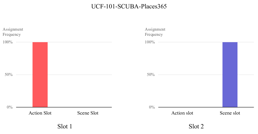
Figure 7: Slot assignments frequency on UCF-101-SCUBA-Places365. We demonstrate the frequency of the slot assignment as either the action slot or the scene slot. In this experiment, we have two slots before assignment ($K=2$): ‘Slot 1’ and ‘Slot 2’. The result demonstrates that each slot performs a singular role, and the representations of the slots are well-disentangled.

Table 8: Downstream task performance across multiple datasets. We report top-1 accuracy. All models are pre-trained on the Kinetics-400 dataset. The best H.M. number is highlighted. SSV2 denotes the Something-Something-V2 dataset.

Supervision	Training Strategy	Method	Temporal-biased			Static-biased
5
8
			Diving48	SSV2		UCF-101	SUN397	H.M.
Action	Naive	Action ViT	81.5	74.2		98.5	69.8	79.6
		Action ViT w/ Aug.	81.6	74.5		98.5	68.4	79.3
Action	Scene Debiasing	BE [67]	81.9	74.5		98.3	69.8	79.8
		FAME [19]	80.6	74.2		98.3	69.4	79.3
Action & Scene	Disentangle	Two-Token	80.1	73.7		98.2	73.5	80.3
		DEVIAS (sum.)	81.6	74.6		98.0	71.4	80.2
		DEVIAS (concat.)	82.4	74.8		98.0	72.1	80.7

E.4 Qualitative results

We provide additional visualization of slot attention of DEVIAS in Figure 8. We select samples from the validation set of the two datasets: UCF-101 for in-context recognition and ‘HAT-Far’ for out-of-context recognition. In both cases, each slot clearly focuses on its designated region.

Appendix F Downstream Task Performance

We further investigate the downstream task performance of DEVIAS and the compared methods. To this end, we design a transfer learning experiment: using the model weights trained on the source dataset as the initialization, we fine-tune the models on the target datasets. For the target dataset fine-tuning, we use only the cross-entropy loss with action ground-truth labels.

We employ the Kinetics-400 as our source dataset, and the Diving48 [43], Something-Something V2 [28], UCF-101 [60], and SUN397 [74] as our target datasets. We choose multiple datasets with distinct characteristics, including the temporal-biased Diving48 and Something-Something-V2, static-biased UCF-101 and SUN397. For a quick experiment, we use the first 88 classes (0 to 87) out of the 174 classes of the Something-Something-V2 dataset and the first 200 classes out of the 397 classes of the SUN397 dataset.

We compare DEVIAS with naive baselines (Action ViT, Action ViT w/ Aug., Scene ViT), scene debiasing methods (BE [67], FAME [19]), and the disentangling baseline (Two-Token) using the full fine-tuning protocol. For the Two-Token baseline, we aggregate the penultimate layer features by average pooling across the temporal and spatial axes to yield a single feature vector. We feed the feature vector into the classification head. For DEVIAS, we explore two naive fusion methods: i) summation and ii) concatenation. In the DEVIAS fusion methods, we fine-tune the encoder along with the slots from the disentangle module. The sum fusion (i) uses the sum of the action and scene slots as a feature vector as input to the classification head. The concat fusion (ii) uses a feature vector obtained by concatenating the action and scene slots. We show the results in Table 8 and summarize the hyperparameters used in Table 11. Compared to the baselines, DEVIAS shows favorable performance on the downstream tasks across the temporal-biased and the static-biased tasks. We expect enhanced performances on the downstream tasks with more advanced fusion methods. We leave the investigation on more advanced fusion methods as our future work.

Input Frame

Action Slot

Scene Slot

Input Frame

Action Slot

Scene Slot

Input Frame

Action Slot

Scene Slot

Input Frame

Action Slot

Scene Slot

(a) In-Context

(b) Out-of-Context

Figure 8: Visualization of DEVIAS slot attention map. (a) In-Context video from UCF-101 [60], (b) Out-of-Context video from HAT Far [13]. Each slot attends to action and scene regions well across frames regardless of in-context or out-of-context. Best viewed with zoom and color.

Table 9: Hyperparameters used for training the scene model on Places365.

Config	Places365
Optimizer	AdamW [49]
Base learning rate	5e-4
Weight decay	0.05
Optimizer momentum	$\beta_{1},\beta_{2}=0.9,0.999$ [9]
Per GPU batch size	32
Drop path	0.1
Mixup [81]	0.8
Cutmix [80]	1.0
Smoothing [61]	0.1
Flip augmentation	✓
Update frequency	2
Learning rate schedule	cosine decay [48]
Warmup epochs	5
Layer-wise learning rate decay	0.65
Training epochs	100

Table 10: Hyperparameters used for training the Scene ViT on each dataset.

Config	UCF-101	Kinetics-400
Optimizer	AdamW [49]	AdamW
Base learning rate	5e-4	1e-3
Weight decay	0.05	0.05
Optimizer momentum	$\beta_{1},\beta_{2}=0.9,0.999$ [9]	$\beta_{1},\beta_{2}=0.9,0.999$
Per GPU batch size	12	12
Drop path	0.2	0.1
Color jitter	0.4	0.4
Flip augmentation	✓	✓
Mixup [81]	$\times$	$\times$
Cutmix [80]	$\times$	$\times$
Random erasing [84]	$\times$	$\times$
Layer-wise learning rate decay [4]	0.75	0.75
Learning rate schedule	cosine decay [48]	cosine decay
Warmup epochs	5	5
Training epochs	100	100

Table 11: Hyperparameters used for the downstream task fine-tuning on each taget dataset.

Config	Diving48	SSV2	UCF-101	SUN397
Optimizer	AdamW [49]	AdamW	AdamW	AdamW
Base learning rate	5e-4	5e-4	5e-4	5e-4
Weight decay	0.05	0.05	0.05	0.05
Optimizer momentum	$\beta_{1},\beta_{2}=0.9,0.999$ [9]	$\beta_{1},\beta_{2}=0.9,0.999$	$\beta_{1},\beta_{2}=0.9,0.999$	$\beta_{1},\beta_{2}=0.9,0.999$
Per GPU batch size	12	12	12	12
Drop path	0.1	0.1	0.1	0.1
Color jitter	0.4	0.4	0.4	0.4
Flip augmentation	✓	$\times$	✓	✓
Mixup [81]	$\times$	$\times$	$\times$	$\times$
Cutmix [80]	$\times$	$\times$	$\times$	$\times$
Random erasing [84]	$\times$	$\times$	$\times$	$\times$
Layer-wise learning rate decay [4]	0.75	0.75	0.75	0.75
Learning rate schedule	cosine decay [48]	cosine decay	cosine decay	cosine decay
Warmup epochs	5	5	5	5
Training epochs	50	50	50	50

Table 12: Hyperparameters used for the linear probe experiments.

Config	UCF-101	Kinetics-400
Optimizer	AdamW [49]	AdamW
Base learning rate	1e-3	1e-3
Weight decay	0.05	0.05
Optimizer momentum	$\beta_{1},\beta_{2}=0.9,0.999$ [9]	$\beta_{1},\beta_{2}=0.9,0.999$
Per GPU batch size	24	16
Color jitter	0.4	0.4
Flip augmentation	✓	✓
Mixup [81]	$\times$	$\times$
Cutmix [80]	$\times$	$\times$
Random erasing [84]	$\times$	$\times$
Learning rate schedule	cosine decay [48]	cosine decay
Warmup epochs	5	5
Training epochs	50	50

Table 13: Hyperparameters used for training the Action ViT, One-Token, and Two-Token baselines on each dataset.

Config	UCF-101	Kinetics-400
Optimizer	AdamW [49]	AdamW
Base learning rate	5e-4	1e-3
Weight decay	0.05	0.05
Optimizer momentum	$\beta_{1},\beta_{2}=0.9,0.999$ [9]	$\beta_{1},\beta_{2}=0.9,0.999$
Per GPU batch size	12	12
Drop out	0.5	0.0
Drop path	0.2	0.1
Color jitter	0.4	0.4
Flip augmentation	✓	✓
Mixup [81]	$\times$	$\times$
Cutmix [80]	$\times$	$\times$
Random erasing [84]	$\times$	$\times$
Layer-wise learning rate decay [4]	0.75	0.75
Learning rate schedule	cosine decay [48]	cosine decay
Warmup epochs	5	5
Training epochs	100	100

Table 14: Hyperparameters used for training the Action ViT w/ Aug. on each dataset.

Config	UCF-101	Kinetics-400
Optimizer	AdamW [49]	AdamW
Base learning rate	5e-4	1e-3
Weight decay	0.05	0.05
Optimizer momentum	$\beta_{1},\beta_{2}=0.9,0.999$ [9]	$\beta_{1},\beta_{2}=0.9,0.999$
Per GPU batch size	12	12
Drop out	0.5	0.0
Drop path	0.2	0.1
Color jitter	0.4	0.4
Flip augmentation	✓	✓
Mixup [81]	0.8	0.8
Cutmix [80]	1.0	1.0
Random erasing [84]	0.25	0.25
Layer-wise learning rate decay [4]	0.75	0.75
Learning rate schedule	cosine decay [48]	cosine decay
Warmup epochs	5	5
Training epochs	100	100

Table 15: Hyperparameters used for BE [67] and training the Two-Token w/ BE on each dataset.

Config	UCF-101	Kinetics-400
Optimizer	AdamW [49]	AdamW
Base learning rate	5e-4	1e-3
Weight decay	0.05	0.05
Optimizer momentum	$\beta_{1},\beta_{2}=0.9,0.999$ [9]	$\beta_{1},\beta_{2}=0.9,0.999$
Per GPU batch size	12	12
Drop out	0.5	0.0
Drop path	0.2	0.1
Color jitter	0.4	0.4
Flip augmentation	✓	✓
Mixup [81]	$\times$	$\times$
Cutmix [80]	$\times$	$\times$
Random erasing [84]	$\times$	$\times$
Mixing weight	$\sim\text{Uniform}(0,0.3)$	$\sim\text{Uniform}(0,0.3)$
$\rho$	0.5	0.5
Layer-wise learning rate decay [4]	0.75	0.75
Learning rate schedule	cosine decay [48]	cosine decay
Warmup epochs	5	5
Training epochs	100	100

Table 16: Hyperparameters used for FAME [19] and training the Two-Token w/ FAME on each dataset.

Config	UCF-101	Kinetics-400
Optimizer	AdamW [49]	AdamW
Base learning rate	5e-4	1e-3
Weight decay	0.05	0.05
Optimizer momentum	$\beta_{1},\beta_{2}=0.9,0.999$ [9]	$\beta_{1},\beta_{2}=0.9,0.999$
Per GPU batch size	12	12
Drop out	0.5	0.0
Drop path	0.2	0.1
Color jitter	0.4	0.4
Flip augmentation	✓	✓
Mixup [81]	$\times$	$\times$
Cutmix [80]	$\times$	$\times$
Random erasing [84]	$\times$	$\times$
$\tau$,$\rho$	0.5,0.5	0.5,0.5
Layer-wise learning rate decay [4]	0.75	0.75
Learning rate schedule	cosine decay [48]	cosine decay
Warmup epochs	5	5
Training epochs	100	100

Table 17: Hyperparameters used for training DEVIAS on each dataset.

Config	UCF-101	Kinetics-400
Optimizer	AdamW [49]	AdamW
Base learning rate	5e-4	5e-4
Weight decay	0.05	0.05
Optimizer momentum	$\beta_{1},\beta_{2}=0.9,0.999$ [9]	$\beta_{1},\beta_{2}=0.9,0.999$
Per GPU batch size	12	12
Drop out	0.5	0.0
Drop path	0.2	0.1
Color jitter	0.4	0.4
Flip augmentation	✓	✓
Mixup [81]	$\times$	$\times$
Cutmix [80]	$\times$	$\times$
Random erasing [84]	$\times$	$\times$
Layer-wise learning rate decay [4]	0.75	0.75
Learning rate schedule	cosine decay [48]	cosine decay
Warmup epochs	5	5
Mask extractor	FAME [19]	FAME
$\tau$,$\rho$	0.3,0.4	0.5,0.8
$\alpha,\beta,\gamma$	1,1,1	1,1,1
M	4	8
Disentangle module learning scale	0.1	0.1
K	2	2
Training epochs	100	100

References

- [1] Anurag Arnab, Mostafa Dehghani, Georg Heigold, Chen Sun, Mario Lučić, and Cordelia Schmid. Vivit: A video vision transformer. In ICCV, 2021.
- [2] Jimmy Lei Ba, Jamie Ryan Kiros, and Geoffrey E. Hinton. Layer normalization, 2016.
- [3] Hyojin Bahng, Sanghyuk Chun, Sangdoo Yun, Jaegul Choo, and Seong Joon Oh. Learning de-biased representations with biased representations. In ICML, 2020.
- [4] Hangbo Bao, Li Dong, Songhao Piao, and Furu Wei. Beit: Bert pre-training of image transformers. arXiv preprint arXiv:2106.08254, 2021.
- [5] Gedas Bertasius, Heng Wang, and Lorenzo Torresani. Is space-time attention all you need for video understanding? In ICML, 2021.
- [6] Sarthak Bhagat, Shagun Uppal, Zhuyun Yin, and Nengli Lim. Disentangling multiple features in video sequences using gaussian processes in variational autoencoders. In ECCV, 2020.
- [7] Nicolas Carion, Francisco Massa, Gabriel Synnaeve, Nicolas Usunier, Alexander Kirillov, and Sergey Zagoruyko. End-to-end object detection with transformers. In ECCV, 2020.
- [8] Joao Carreira and Andrew Zisserman. Quo Vadis, Action Recognition? A New Model and the Kinetics Dataset. In CVPR, 2018.
- [9] Mark Chen, Alec Radford, Rewon Child, Jeffrey Wu, Heewoo Jun, David Luan, and Ilya Sutskever. Generative pretraining from pixels. In ICML, 2020.
- [10] Xi Chen, Yan Duan, Rein Houthooft, John Schulman, Ilya Sutskever, and Pieter Abbeel. Infogan: Interpretable representation learning by information maximizing generative adversarial nets. In NeurIPS, 2016.
- [11] Jinwoo Choi, Chen Gao, Joseph CE Messou, and Jia-Bin Huang. Why can’t i dance in the mall? learning to mitigate scene bias in action recognition. In NeurIPS, 2019.
- [12] Jinwoo Choi, Gaurav Sharma, Samuel Schulter, and Jia-Bin Huang. Shuffle and attend: Video domain adaptation. In ECCV, 2020.
- [13] Jihoon Chung, Yu Wu, and Olga Russakovsky. Enabling detailed action recognition evaluation through video dataset augmentation. In NeurIPS, 2022.
- [14] Ioana Croitoru, Simion-Vlad Bogolin, and Marius Leordeanu. Unsupervised learning from video to detect foreground objects in single images. In CVPR, 2017.
- [15] Katherine Crowson, Stella Biderman, Daniel Kornis, Dashiell Stander, Eric Hallahan, Louis Castricato, and Edward Raff. Vqgan-clip: Open domain image generation and editing with natural language guidance. In ECCV, 2022.
- [16] Jia Deng, Wei Dong, Richard Socher, Li-Jia Li, Kai Li, and Li Fei-Fei. Imagenet: A large-scale hierarchical image database. In CVPR, 2009.
- [17] Emily L Denton et al. Unsupervised learning of disentangled representations from video. In NeurIPS, 2017.
- [18] Ali Diba, Mohsen Fayyaz, Vivek Sharma, Manohar Paluri, Jürgen Gall, Rainer Stiefelhagen, and Luc Van Gool. Large scale holistic video understanding. In ECCV, 2020.
- [19] Shuangrui Ding, Maomao Li, Tianyu Yang, Rui Qian, Haohang Xu, Qingyi Chen, Jue Wang, and Hongkai Xiong. Motion-aware contrastive video representation learning via foreground-background merging. In CVPR, 2022.
- [20] Jeff Donahue, Lisa Anne Hendricks, Marcus Rohrbach, Subhashini Venugopalan, Sergio Guadarrama, Kate Saenko, and Trevor Darrell. Long-term Recurrent Convolutional Networks for Visual Recognition and Description. In CVPR, 2015.
- [21] Alexey Dosovitskiy, Lucas Beyer, Alexander Kolesnikov, Dirk Weissenborn, Xiaohua Zhai, Thomas Unterthiner, Mostafa Dehghani, Matthias Minderer, Georg Heigold, Sylvain Gelly, Jakob Uszkoreit, and Neil Houlsby. An image is worth 16x16 words: Transformers for image recognition at scale. In ICLR, 2021.
- [22] Bernard Ghanem Fabian Caba Heilbron, Victor Escorcia and Juan Carlos Niebles. Activitynet: A large-scale video benchmark for human activity understanding. In CVPR, 2015.
- [23] Haoqi Fan, Bo Xiong, Karttikeya Mangalam, Yanghao Li, Zhicheng Yan, Jitendra Malik, and Christoph Feichtenhofer. Multiscale vision transformers. In ICCV, 2021.
- [24] Christoph Feichtenhofer. X3d: Expanding architectures for efficient video recognition. In CVPR, 2020.
- [25] Christoph Feichtenhofer, Haoqi Fan, Jitendra Malik, and Kaiming He. Slowfast networks for video recognition. In ICCV, 2019.
- [26] Rohit Girdhar, Mannat Singh, Nikhila Ravi, Laurens van der Maaten, Armand Joulin, and Ishan Misra. Omnivore: A Single Model for Many Visual Modalities. In CVPR, 2022.
- [27] Shreyank N Gowda, Marcus Rohrbach, Frank Keller, and Laura Sevilla-Lara. Learn2augment: learning to composite videos for data augmentation in action recognition. In ECCV, 2022.
- [28] Raghav Goyal, Samira Ebrahimi Kahou, Vincent Michalski, Joanna Materzynska, Susanne Westphal, Heuna Kim, Valentin Haenel, Ingo Fruend, Peter Yianilos, Moritz Mueller-Freitag, et al. The” something something” video database for learning and evaluating visual common sense. In ICCV, 2017.
- [29] Kaiming He, Xinlei Chen, Saining Xie, Yanghao Li, Piotr Dollár, and Ross Girshick. Masked autoencoders are scalable vision learners. In CVPR, 2022.
- [30] Dan Hendrycks and Kevin Gimpel. Gaussian error linear units (gelus). arXiv preprint arXiv:1606.08415, 2016.
- [31] Roei Herzig, Elad Ben-Avraham, Karttikeya Mangalam, Amir Bar, Gal Chechik, Anna Rohrbach, Trevor Darrell, and Amir Globerson. Object-region video transformers. In CVPR, 2022.
- [32] Irina Higgins, Loic Matthey, Arka Pal, Christopher Burgess, Xavier Glorot, Matthew Botvinick, Shakir Mohamed, and Alexander Lerchner. beta-vae: Learning basic visual concepts with a constrained variational framework. In ICLR, 2016.
- [33] Jun-Ting Hsieh, Bingbin Liu, De-An Huang, Li F Fei-Fei, and Juan Carlos Niebles. Learning to decompose and disentangle representations for video prediction. In NeurIPS, 2018.
- [34] Shuiwang Ji, Wei Xu, Ming Yang, and Kai Yu. 3D convolutional neural networks for human action recognition. TPAMI, 2013.
- [35] Andrej Karpathy, George Toderici, Sanketh Shetty, Thomas Leung, Rahul Sukthankar, and Li Fei-Fei. Large-scale video classification with convolutional neural networks. In CVPR, 2014.
- [36] Will Kay, Joao Carreira, Karen Simonyan, Brian Zhang, Chloe Hillier, Sudheendra Vijayanarasimhan, Fabio Viola, Tim Green, Trevor Back, Paul Natsev, et al. The kinetics human action video dataset. arXiv preprint arXiv:1705.06950, 2017.
- [37] Dongwon Kim, Namyup Kim, and Suha Kwak. Improving cross-modal retrieval with set of diverse embeddings. In CVPR, 2023.
- [38] Hildegard Kuehne, Hueihan Jhuang, Estíbaliz Garrote, Tomaso Poggio, and Thomas Serre. Hmdb: a large video database for human motion recognition. In ICCV, 2011.
- [39] Harold W Kuhn. The hungarian method for the assignment problem. Naval research logistics quarterly, 1955.
- [40] Tejas D Kulkarni, William F Whitney, Pushmeet Kohli, and Josh Tenenbaum. Deep convolutional inverse graphics network. In NeurIPS, 2015.
- [41] Zihang Lai, Sifei Liu, Alexei A Efros, and Xiaolong Wang. Video autoencoder: self-supervised disentanglement of static 3d structure and motion. In CVPR, 2021.
- [42] Haoxin Li, Yuan Liu, Hanwang Zhang, and Boyang Li. Mitigating and evaluating static bias of action representations in the background and the foreground. In ICCV, 2023.
- [43] Yingwei Li, Yi Li, and Nuno Vasconcelos. Resound: Towards action recognition without representation bias. In ECCV, 2018.
- [44] Ji Lin, Chuang Gan, and Song Han. TSM: Temporal Shift Module for Efficient Video Understanding. In ICCV, 2019.
- [45] Xunyu Lin, Victor Campos, Xavier Giro-i Nieto, Jordi Torres, and Cristian Canton Ferrer. Disentangling motion, foreground and background features in videos. arXiv preprint arXiv:1707.04092, 2017.
- [46] Francesco Locatello, Dirk Weissenborn, Thomas Unterthiner, Aravindh Mahendran, Georg Heigold, Jakob Uszkoreit, Alexey Dosovitskiy, and Thomas Kipf. Object-centric learning with slot attention. In NeurIPS, 2020.
- [47] Fuchen Long, Zhaofan Qiu, Yingwei Pan, Ting Yao, Jiebo Luo, and Tao Mei. Stand-alone inter-frame attention in video models. In CVPR, 2022.
- [48] Ilya Loshchilov and Frank Hutter. Sgdr: Stochastic gradient descent with warm restarts. arXiv preprint arXiv:1608.03983, 2016.
- [49] Ilya Loshchilov and Frank Hutter. Decoupled weight decay regularization. In ICLR, 2019.
- [50] Armand Comas Massagué, Chi Zhang, Zlatan Feric, Octavia I Camps, and Rose Yu. Learning disentangled representations of videos with missing data. In NeurIPS, 2020.
- [51] Leland McInnes, John Healy, and James Melville. Umap: Uniform manifold approximation and projection for dimension reduction. arXiv preprint arXiv:1802.03426, 2018.
- [52] Antoine Miech, Jean-Baptiste Alayrac, Ivan Laptev, Josef Sivic, and Andrew Zisserman. Rareact: A video dataset of unusual interactions. arxiv:2008.01018, 2020.
- [53] Joe Yue-Hei Ng, Matthew Hausknecht, Sudheendra Vijayanarasimhan, Oriol Vinyals, Rajat Monga, and George Toderici. Beyond Short Snippets: Deep Networks for Video Classification. In CVPR, 2015.
- [54] Mandela Patrick, Dylan Campbell, Yuki Asano, Ishan Misra, Florian Metze, Christoph Feichtenhofer, Andrea Vedaldi, and Joao F Henriques. Keeping your eye on the ball: Trajectory attention in video transformers. In NeurIPS, 2021.
- [55] Rui Qian, Shuangrui Ding, Xian Liu, and Dahua Lin. Static and dynamic concepts for self-supervised video representation learning. In ECCV, 2022.
- [56] Jamie Ray, Heng Wang, Du Tran, Yufei Wang, Matt Feiszli, Lorenzo Torresani, and Manohar Paluri. Scenes-objects-actions: A multi-task, multi-label video dataset. In ECCV, 2018.
- [57] Arka Sadhu, Tanmay Gupta, Mark Yatskar, Ram Nevatia, and Aniruddha Kembhavi. Visual semantic role labeling for video understanding. In CVPR, 2021.
- [58] Aadarsh Sahoo, Rutav Shah, Rameswar Panda, Kate Saenko, and Abir Das. Contrast and mix: Temporal contrastive video domain adaptation with background mixing. In NeurIPS, 2021.
- [59] Karen Simonyan and Andrew Zisserman. Two-stream convolutional networks for action recognition in videos. In NeurIPS, 2014.
- [60] Khurram Soomro, Amir Roshan Zamir, and Mubarak Shah. Ucf101: A dataset of 101 human actions classes from videos in the wild. arXiv preprint arXiv:1212.0402, 2012.
- [61] Christian Szegedy, Vincent Vanhoucke, Sergey Ioffe, Jon Shlens, and Zbigniew Wojna. Rethinking the inception architecture for computer vision. In CVPR, 2016.
- [62] Zhan Tong, Yibing Song, Jue Wang, and Limin Wang. Videomae: Masked autoencoders are data-efficient learners for self-supervised video pre-training. In NeurIPS, 2022.
- [63] Du Tran, Lubomir Bourdev, Rob Fergus, Lorenzo Torresani, and Manohar Paluri. Learning spatiotemporal features with 3d convolutional networks. In ICCV, 2015.
- [64] Du Tran, Heng Wang, Lorenzo Torresani, Jamie Ray, Yann LeCun, and Manohar Paluri. A closer look at spatiotemporal convolutions for action recognition. In CVPR, 2018.
- [65] Luan Tran, Xi Yin, and Xiaoming Liu. Disentangled representation learning gan for pose-invariant face recognition. In CVPR, 2017.
- [66] Ruben Villegas, Jimei Yang, Seunghoon Hong, Xunyu Lin, and Honglak Lee. Decomposing motion and content for natural video sequence prediction. In ICLR, 2017.
- [67] Jinpeng Wang, Yuting Gao, Ke Li, Yiqi Lin, Andy J Ma, Hao Cheng, Pai Peng, Feiyue Huang, Rongrong Ji, and Xing Sun. Removing the background by adding the background: Towards background robust self-supervised video representation learning. In CVPR, 2021.
- [68] Jiangliu Wang, Jianbo Jiao, Linchao Bao, Shengfeng He, Yunhui Liu, and Wei Liu. Self-supervised spatio-temporal representation learning for videos by predicting motion and appearance statistics. In CVPR, 2019.
- [69] Xiaolong Wang, Ross Girshick, Abhinav Gupta, and Kaiming He. Non-local neural networks. In CVPR, 2018.
- [70] Yaohui Wang, Piotr Bilinski, Francois Bremond, and Antitza Dantcheva. G3an: Disentangling appearance and motion for video generation. In CVPR, 2020.
- [71] Yang Wang and Minh Hoai. Pulling actions out of context: Explicit separation for effective combination. In CVPR, 2018.
- [72] Philippe Weinzaepfel and Grégory Rogez. Mimetics: Towards understanding human actions out of context. IJCV, 2021.
- [73] Chao-Yuan Wu, Yanghao Li, Karttikeya Mangalam, Haoqi Fan, Bo Xiong, Jitendra Malik, and Christoph Feichtenhofer. Memvit: Memory-augmented multiscale vision transformer for efficient long-term video recognition. In CVPR, 2022.
- [74] Jianxiong Xiao, James Hays, Krista A. Ehinger, Aude Oliva, and Antonio Torralba. Sun database: Large-scale scene recognition from abbey to zoo. In CVPR, 2010.
- [75] Christopher Xie, Yu Xiang, Zaid Harchaoui, and Dieter Fox. Object discovery in videos as foreground motion clustering. In CVPR, 2019.
- [76] Enze Xie, Wenhai Wang, Zhiding Yu, Anima Anandkumar, Jose M Alvarez, and Ping Luo. Segformer: Simple and efficient design for semantic segmentation with transformers. In NeurIPS, 2021.
- [77] Saining Xie, Chen Sun, Jonathan Huang, Zhuowen Tu, and Kevin Murphy. Rethinking spatiotemporal feature learning for video understanding. In ECCV, 2018.
- [78] Xianglei Xing, Ruiqi Gao, Tian Han, Song-Chun Zhu, and Ying Nian Wu. Deformable generator networks: unsupervised disentanglement of appearance and geometry. TPAMI, 2020.
- [79] Shen Yan, Xuehan Xiong, Anurag Arnab, Zhichao Lu, Mi Zhang, Chen Sun, and Cordelia Schmid. Multiview transformers for video recognition. In CVPR, 2022.
- [80] Sangdoo Yun, Dongyoon Han, Seong Joon Oh, Sanghyuk Chun, Junsuk Choe, and Youngjoon Yoo. Cutmix: Regularization strategy to train strong classifiers with localizable features. In CVPR, 2019.
- [81] Hongyi Zhang, Moustapha Cisse, Yann N Dauphin, and David Lopez-Paz. mixup: Beyond empirical risk minimization. In ICLR, 2017.
- [82] Ziyuan Zhang, Luan Tran, Xi Yin, Yousef Atoum, Xiaoming Liu, Jian Wan, and Nanxin Wang. Gait recognition via disentangled representation learning. In CVPR, 2019.
- [83] Yue Zhao, Yuanjun Xiong, and Dahua Lin. Recognize actions by disentangling components of dynamics. In CVPR, 2018.
- [84] Zhun Zhong, Liang Zheng, Guoliang Kang, Shaozi Li, and Yi Yang. Random erasing data augmentation. In AAAI, 2020.
- [85] Bolei Zhou, Alex Andonian, Aude Oliva, and Antonio Torralba. Temporal Relational Reasoning in Videos. In ECCV, 2018.
- [86] Bolei Zhou, Agata Lapedriza, Aditya Khosla, Aude Oliva, and Antonio Torralba. Places: A 10 million image database for scene recognition. TPAMI, 2017.
- [87] Yuliang Zou, Jinwoo Choi, Qitong Wang, and Jia-Bin Huang. Learning representational invariances for data-efficient action recognition. Computer Vision and Image Understanding, 2023.