Non-Cross Diffusion for Semantic Consistency

Abstract

In diffusion models, deviations from a straight generative flow are a common issue, resulting in semantic inconsistencies and suboptimal generations. To address this challenge, we introduce ‘Non-Cross Diffusion’, an innovative approach in generative modeling for learning ordinary differential equation (ODE) models. Our methodology strategically incorporates an ascending dimension of input to effectively connect points sampled from two distributions with uncrossed paths. This design is pivotal in ensuring enhanced semantic consistency throughout the inference process, which is especially critical for applications reliant on consistent generative flows, including various distillation methods and deterministic sampling, which are fundamental in image editing and interpolation tasks.

Our empirical results demonstrate the effectiveness of Non-Cross Diffusion, showing a substantial reduction in semantic inconsistencies at different inference steps and a notable enhancement in the overall performance of diffusion models.

1 Introduction

Diffusion models, as delineated in recent studies [23, 11, 4, 17, 19, 24, 25], have exhibited remarkable capabilities in image synthesis, bolstering numerous applications such as text-to-image generation [16, 21], image editing [1, 16, 2, 26], and image inpainting [1, 18]. A key characteristic of these models is their multi-step generative process, which not only allows for correction of the diffusion path [25] but also enhances controllability [5, 7].

Despite these advancements, the inference process in diffusion models typically involves a specific flow, whereas the training process entails random step selections from multiple flows. This randomness often results in a given training step correlating with diverse flows, creating ambiguity in target identification from the network’s perspective, as depicted in Fig. 1(a). We term this phenomenon ‘xFlow’.

xFlow’s emergence during training can hinder the model’s optimization at certain steps, leading to a spectrum of generative issues. Notably, it challenges the model’s ability to generate samples via a straight flow, compromising deterministic sampling across varying step counts, as shown in Fig. 1(c). It also complicates predicting later sampling steps from earlier ones, limiting the effectiveness of reward models [30] and guided models [4]. Moreover, in the context of distillation, which typically adopts a progressive approach, xFlow can introduce misleading signals, as evidenced in Rectified Flow [14]. Perhaps most critically, xFlow can lead to the generation of Out-Of-Distribution (OOD) samples or low-quality samples, especially as sampling step size increases, as illustrated in Fig. 1(d-e).

In this paper, we propose a novel training strategy aimed at resolving the xFlow challenge in diffusion models. Our method centers on augmenting the input dimensionality to these models, a change that effectively prevents flow crossing. As depicted in Fig. 1(a), the issue at hand arises when two flows intersect, creating ambiguity; the input to the network (for instance, a noisy image) remains constant, yet it is associated with multiple potential targets (such as distinct noises originating from different images). To address this, our approach entails predicting the flow itself during the training phase, as shown in Fig. 1(b). Notably, we utilize the noise predicted by the network as the flow’s endpoint, incorporating this element into the model’s input. This technique sidesteps the pitfall of using groundtruth noise as input, which would otherwise result in trivial training solutions devoid of substantive learning. For practical implementation, we found ControlNet [31] particularly effective in this context. Additionally, our methodology integrates a bootstrap approach reminiscent of Analog bits [3], which significantly enhances our model’s optimization and effectively narrows the gap between training and inference phases.”

To evaluate our approach, we introduce the Inference Flow Consistency ($\operatorname{IFC}$) metric, reflecting xFlow severity. We also utilize Inception Score (IS) [22] and Fréchet Inception Distance (FID) [9] for assessing generation quality. Our models, trained from scratch and compared against baselines on Cifar-10 [13], demonstrate not only an avoidance of xFlow but also an enhancement in generation quality. The contributions of this paper include:

• We identify a widespread phenomenon in diffusion models, termed xFlow, leading to non-straight flow during inference that may generate OOD or suboptimal samples.

• We attribute xFlow’s origins to the instability of the target during the training process. Accordingly, we introduce the Non-Cross Diffusion, a novel training and inference pipeline to mitigate the xFlow problem by enhancing input dimensionality.

• Our experiments on both a toy model and the Cifar-10 dataset demonstrate that our method not only improves the proposed $\operatorname{IFC}$ metric by addressing xFlow, but also significantly enhances other image evaluation metrics, such as IS and FID.

2 Related work

2.1 Diffusion models

Diffusion models, as generative models, learn the reverse denoising process from Gaussian noise to image distribution, achieved through either Markov [11] or non-Markov operations [23]. They are favored over other generative models like GAN [8] and VAE [27] due to their training stability and superior generation quality. Subsequent enhancements to these models primarily concern varied network architectures [12], noise schedulers or losses [17], transition from image space diffusion to latent space [19], and improved sampling techniques [15], with little attention to the xFlow during training. Rectified Flow [14] noted the mismatch in sampling across different inference steps, a significant distillation issue, but did not analyze it further. Instead, they proposed a workaround using a 2-rectified flow to fit another model to a non-crossing flow between source and target distributions, which depends on a well-trained diffusion model and requires additional retraining. Our paper is the first to examine xFlow in diffusion and offer solutions.

2.2 Conditional Image Generation

Conditioning techniques are instrumental in managing generated content [19, 6, 29, 28]. For diffusion models, [25] proposes classifier guidance, which is an efficient method to balance controllability and fidelity using the gradients from a classifier, while classifier-free guidance [10], being another important conditioning technique to diffusion models, trains both conditional and unconditional diffusion models, and combining their score to achieve better controllability. ControlNet [31] employs pretrained encoding layers from billions of images as a backbone to learn diverse conditional controls, which is an architecture adopted in this paper. Analog Bits [3] introduces a technique that conditions the model on its own previously generated samples during iterative sampling, akin to our work. However, Analog Bits mainly aims to enhance sample quality by reusing the previous target, while our focus is to introduce a condition in the training flow to prevent crossing issues.

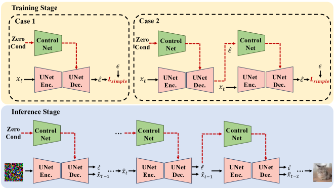
Figure 2: The overview of non-cross diffusion. Training stage: The training phase involves two cases. In Case1, we utilize $\mathbf{0}$ as the condition and calculate loss function $L_{simple}$ as defined in Eq. 5. For Case2, we first compute $\hat{\epsilon}$ using $\mathbf{0}$ as condition. Subsequently, $\hat{\epsilon}$ is employed as the condition to calculate $L_{simple}$. Throughout the training process, Case1 is applied with a fixed probability $p$; otherwise, Case2 is implemented. Inference stage: During the inference phase, 0 is used as the condition in the initial denoising step. This is followed by iterative utilization of the estimated noise from the previous step as the condition for subsequent steps.

3 Method

In this section, we start with a brief review of the formulation of DDPM [11]. Next, we show the drawback of baseline flow and then introduce Non-Cross Diffusion to avoid crossing by ascending dimension of input. At last, we present our training and inference flow of Non-Cross Diffusion.

3.1 Preliminary

Given a data distribution $x_{0}\sim q(x_{0})$, we define a forward noising process $q$ which produces latent ${x_{1},\ldots,x_{T}}$ by adding Gaussian noise at time with variance $\beta_{t}\in(0,1)$ as follows:

$$q(x_{1},\ldots,x_{T})\coloneqq\prod_{t=1}^{T}q(x_{t}|x_{t-1}),$$ (1)

$$q(x_{t}|x_{t-1})\coloneqq\mathcal{N}(x_{t};\sqrt{1-\beta_{t}}x_{t-1},\beta_{t}\mathbf{I}).$$ (2)

With $\alpha_{t}=1-\beta_{t}$ and $\bar{\alpha}_{t}=\prod_{s=0}^{t}\alpha_{s}$, we write the marginal $q(x_{t}|x_{0})$ through Eq. 2 as follows:

$$q(x_{t}|x_{0})\coloneqq\mathcal{N}(x_{t},\sqrt{\bar{\alpha}_{t}}x_{0},(1-\bar{\alpha}_{t})\mathbf{I}),$$ (3)

$$x_{t}=\sqrt{\bar{\alpha}_{t}}x_{0}+\sqrt{1-\bar{\alpha}_{t}}\epsilon,$$ (4)

where $\epsilon\sim\mathcal{N}(0,\mathbf{I})$. Using Bayes theorem, we can calculate the posterior $q(x_{t}|x_{t},x_{0})$ in terms of $\tilde{\beta}$ and $\tilde{\mu}_{t}(x_{t},x_{0})$. There are many different ways to parameterize $\mu_{\theta}(x_{t},t)$. DDPM [11] found that predicting $\epsilon$ worked best with a loss function:

$$L_{simple}=E_{t,x_{0},\epsilon}[\|\epsilon-\epsilon_{\theta}(x_{t},t)\|^{2}]$$ (5)

3.2 Understanding Drawbacks of DDPM Flow

Training stage: Given source distribution $\pi_{0}$ and target distribution $\pi_{1}$, we sample two data pairs $(x_{0},x_{T}),(y_{0},y_{T})\sim\pi_{0}\times\pi_{1}$. During the training stage, assume that these two training flows cross at time step $t$, which means:

$$x_{t}=\sqrt{\bar{\alpha}_{t}}x_{0}+\sqrt{1-\bar{\alpha}_{t}}\epsilon_{x},$$ (6)

$$y_{t}=\sqrt{\bar{\alpha}_{t}}y_{0}+\sqrt{1-\bar{\alpha}_{t}}\epsilon_{y},$$ (7)

$$x_{t}=y_{t}.$$ (8)

In the cross point, the two training flow aims to minimize the loss function as follows:

$$\min_{\theta}E_{t,x_{0},\epsilon_{x}}[\|\epsilon_{x}-\epsilon_{\theta}(x_{t},t)\|^{2}],$$ (9)

$$\min_{\theta}E_{t,y_{0},\epsilon_{y}}[\|\epsilon_{y}-\epsilon_{\theta}(y_{t},t)\|^{2}].$$ (10)

Since $x_{t}=y_{t}$, we can rewrite the above target as follows:

$$\min_{\theta}E_{t,z_{t},\epsilon_{x},\epsilon_{y}}[\|\frac{(\epsilon_{x}+\epsilon_{y})}{2}-\epsilon_{\theta}(z_{t},t)\|^{2}],$$ (11)

where $z_{t}=x_{t}=y_{t}$. This implies that for the cross point, the model is given an incorrect target and will lead to the generation of an OOD sample.

Inference stage. As illustrated in Fig. 1, the decision to change direction during the inference process is contingent on the timestep of inference. Specifically, a larger inference step correlates with a smaller stride, resulting in only a slight influence from the cross point on the inference flow, typically insufficient to alter its direction. Conversely, a smaller inference step is associated with a larger stride, significantly impacting the inference flow due to the cross point and consequently altering its direction. This alteration can lead to the generation of inconsistent or OOD samples. Such a phenomenon underscores the dependence of the generated image on the inference step, potentially reducing the determinism of the diffusion model.

3.3 Selection of Condition

In this section, we delve deeper into our proposed method, which focuses on avoiding the intersection of training flows in a unique and effective manner. The core principle behind this method is derived from a basic geometrical concept: any two distinct lines in a plane can intersect at most once. By leveraging this idea, we aim to ensure that different training flows do not cross each other, thereby maintaining the integrity and distinctiveness of each flow.

To operationalize this concept, our approach involves the use of concatenation of different points in the training flow. Specifically, by concatenating $x_{t}$ with $x_{i}$, where $i\neq t$, we ensure that two different training flows will not cross. Practically, we sample two data pairs $(x_{0},x_{T}),(y_{0},y_{T})\sim\pi_{0}\times\pi_{1}$, and assume that $x_{t}\neq y_{t}$. Then we have $[x_{i},x_{t}]\neq[y_{i},y_{t}],\forall i\in[0,T]$, which denotes that by ascending dimensions with the noised image in timestep $t$, two training flows will no longer intersect. This strategy effectively creates a multidimensional space where the likelihood of training flows intersecting is significantly reduced.

Given the continuity inherent in diffusion models, we observe that the effectiveness of avoiding crossing points improves when the selected points are farther from these intersections. Thus, we propose to use either initial noise $x_{T}$,i.e. $\epsilon$, or target image $x_{0}$ for dimension ascension.

Furthermore, we find the distance between randomly sampled noise is stable while the distance between image or latent is unstable, which is mainly decided by background or semantic information. Practically, for two randomly sampled noise $n_{1},n_{2}\in\mathbb{R}^{H\times W\times C}$, we have $E[\|n_{1}-n_{2}\|^{2}]=2CHW$. Besides, in the inference stage, we can get the initial noise, but we cannot get the target image. Therefore, we propose to use initial noise $x_{T}$ instead of target image $x_{0}$ as the condition for dimension ascending.

3.4 Proposed Solution

In this section, we delineate the training and inference stages of our Non-Cross Diffusion, emphasizing strategies to enhance model performance and reliability.

Training Stage. The cornerstone of our training strategy is to circumvent trivial solutions and avoid training collapse. To achieve this, we replace the use of initial noise $\epsilon$ with predicted noise $\hat{\epsilon}$. This substitution is critical in refining our model’s predictive accuracy since it can effectively avoid trivial solutions. Furthermore, we introduce a bootstrap strategy in the training stage, which adds robustness to the learning process and avoids misleading of the predicted noise $\hat{\epsilon}$ in the early stage.

As illustrated in Fig. 2, our training objective is formulated as follows:

$$\min_{\theta}E_{t,x_{t},\epsilon,}[\|\epsilon-\epsilon_{\theta}(x_{t},\hat{\epsilon}_{t},t)\|^{2}],$$ (12)

where $x_{t}=\sqrt{\bar{\alpha}_{t}}x_{0}+\sqrt{1-\bar{\alpha}_{t}}\epsilon$. During training, to mitigate the risk of being misled by estimated noise, we set $\hat{\epsilon}_{t}=\mathbf{0}$, i.e. Case1 in Fig. 2, with a fixed probability $p$. At other times,$\hat{\epsilon}_{t}$ is assigned the value of $\epsilon_{\theta}(x_{t},\mathbf{0},t)$,i.e. Case2 in Fig. 2, and we do not backpropagate through estimated noise $\hat{\epsilon}_{t}$.

Inference Stage. As illustrated in Fig. 2, during the inference stage, to alleviate the computational costs, we use estimated noise in the previous step instead of the current step as the condition and iteratively predict $\hat{\epsilon}$ as follows:

$$\hat{\epsilon}_{T}=\epsilon_{\theta}(\hat{x}_{T},\mathbf{0},T),$$ (13)

$$\hat{\epsilon}_{t}=\epsilon_{\theta}(\hat{x}_{t},\hat{\epsilon}_{t+1},t),t<T.$$ (14)

When inference step is large, the discrepancy between $\hat{\epsilon}_{t}$ and $\hat{\epsilon}_{t+1}$ is small, which ensure the performance of our method.

Network Architecture. To effectively utilize $\hat{\epsilon}_{t}$, inspired by ControlNet [31], Non-Cross Diffusion leverage an addictive U-net branch that takes as input $\hat{\epsilon}_{t}$. Besides, we introduce some modifications for optimization. Specifically, we eliminate all zero convolution layers and create a trainable copy of the U-net encoder to encode the condition $\hat{\epsilon}_{t}$. Subsequently, the output from this trainable copy is integrated into the U-net decoder through an addition operation. During the training stage, this entire network is trained from scratch instead of finetuning.

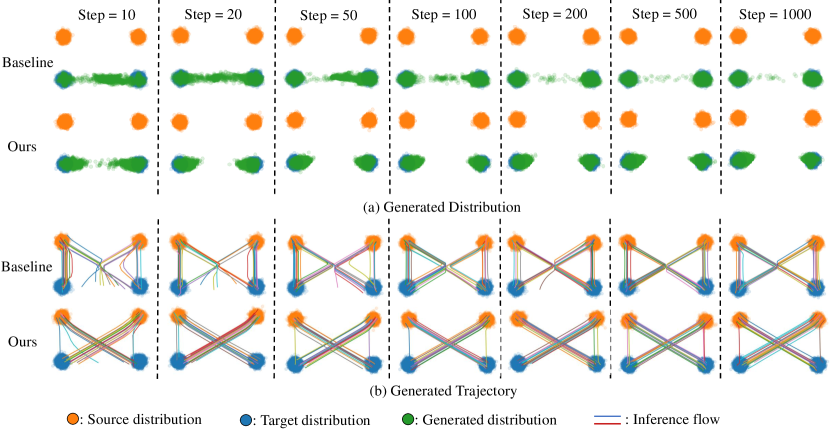
Figure 3: Results of the Toy Model. (a) Comparison of Generated Distributions: This panel illustrates the distributions generated by the baseline model and our proposed model. As the number of inference steps decreases, the baseline model tends to produce a significant number of out-of-distribution (OOD) samples. In contrast, our model effectively mitigates the generation of OOD samples. (b) Trajectory Analysis: This panel compares the generated trajectories of the baseline and our models. The baseline model’s inference flow often redirects at the intersection point, leading to a target OOD distribution as the inference steps decrease. Our method, however, maintains a consistent direction in the inference model, thereby straightening the trajectory.

Inference Flow Consistency. To better evaluate the consistency of the inference flow, we propose a metric by computing the similarity between intermediate generated image $\hat{x}_{0}^{t}$ in timestep $t$ and the final generated image $\hat{x}_{0}$ based on Peak signal-to-noise ratio(PSNR) as follows:

$$\operatorname{IFC}=\frac{1}{T}\sum_{t=0}^{T}PSNR(\hat{x}_{0}^{t},\hat{x}_{0}).$$ (15)

Setting	Method	IS	FID
DDIM-1000	iDDPM	9.02	4.70
	Ours	9.51	2.88
	Ours†	9.34	3.40
DDIM-100	iDDPM	8.99	5.65
	Ours	9.22	3.93
	Ours†	9.15	4.21
DDIM-50	iDDPM	8.89	6.61
	Ours	9.10	5.31
	Ours†	9.05	5.09
DDIM-20	iDDPM	8.59	9.82
	Ours	8.77	9.87
	Ours†	8.84	7.75
DDIM-10	iDDPM	8.20	15.91
	Ours	7.97	20.63
	Ours†	8.50	12.85
DDIM-5	iDDPM	7.09	31.37
	Ours	6.20	50.25
	Ours†	7.45	27.83

Table 1: We compare the performance of baseline and our method. We generate 50k samples using DDIM with inference steps in {1000, 100, 50, 20, 10, 5}. Ours†  use inference strategy similar with training stage. For $\hat{x}_{t}$ ,we first give $\mathbf{0}$ as condition and get estimated noise $\hat{\epsilon_{t}}$, then we take $\hat{\epsilon_{t}}$ as condition and compute denoised image $\hat{x}_{t-1}$.

When the training flow changes direction at a particular timestep, it results in a marked semantic difference between the images generated before and after that timestep, leading to a lower PSNR. By quantifying this using our PSNR-based metric, we can effectively assess and ensure the consistency of the inference process across different stages.

4 Experiment

4.1 Toy Examples

In this section, we follow the setting in Rectified Flow [14]. We start with drawing training dataset $(X_{0},X_{1})\sim\pi_{0}\times\pi_{1}$. Given a sample $\{x_{0}^{i},x_{1}^{i}\}$ drawn from $(X_{0},X_{1})$,for baseline model, we train a 3-layer MLP $v_{\theta}(z,t)$ to transfer source distribution $\pi_{0}$ to target distribution $\pi_{1}$ with l2-loss as follow:

$$\min_{\theta}\|v_{\theta}(x_{t}^{i},t)-(x_{1}^{i}-x_{0}^{i})\|_{2},$$

$$x_{t}^{i}=tx_{1}^{i}+(1-t)x_{0}^{i},t\in[0,1).$$

Our method enhances this approach by incorporating an additional dimension with the estimated target as follows:

$$\min_{\theta}\|v_{\theta}([x_{t}^{i},\hat{c}_{t}^{i}],t)-(x_{1}^{i}-x_{0}^{i})\|_{2},$$

$$\hat{c}_{t}^{i}=\begin{cases}\mathbf{0}&\text{p$\leq$0.5}\\ v_{\theta}([x_{t}^{i},\mathbf{0}],t)&\text{otherwise}\end{cases}$$

with $p$ sampled from a uniform distribution $U(0,1)$. The inference process is also similar to our proposed method, i.e., we use the estimated target in the previous step as the condition.

4.2 Comparison Experiment

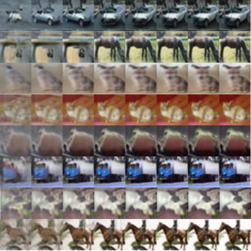
(a) Baseline

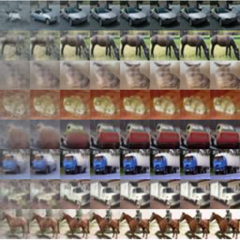
(b) Ours

Figure 4: Here are the generated images using DDIM with inference steps in {5, 10, 20, 50, 100, 1000}. For baseline method, the semantic information of image with small inference step and large inference step could be greatly different, which implies that the inference flow changes its direction at some timesteps.

As depicted in Fig. 3, the inference flow of the baseline model changes direction at the cross point of the two flows. This redirection results from an incorrect loss function, as illustrated in Eq. 11, leading to the generation of OOD samples. Our method, by using the estimated result to introduce an additional dimension, avoids the crossing of training and inference flows. This ensures a consistent direction in the inference flow and effectively prevents the generation of OOD samples.

Implementation Details. We train our models of $32\times 32$ images on Cifar-10 [13]. We evaluate the fidelity of generated samples using IS [22] and FID [9] and the consistency of inference flow using $\operatorname{IFC}$. For model on Cifar-10, we refer to the setting of iDDPM [17] except that we use $L_{simple}$ only and we set the training step to 250k. For baseline model, we train iDDPM[17] from scratch following the original setting except that we set the training step the same as ours, i.e. 250k.

Comparison of Sampling Quality. In Table 1, we present a comparison of our model with a baseline model in generating Cifar-10 images. Our model demonstrates superior performance, showing significant improvements over the baseline, particularly at inference steps in {1000, 100, 50}. However, as the inference steps decrease and stride increases, the difference in estimated noise between successive steps grows. This discrepancy introduces a bias during the inference stage, leading to a decline in performance. To mitigate this bias, we propose using the estimated noise from the current step as a condition. This approach enables our method to enhance the quality of generated images even at smaller inference steps in {20, 10, 5}.

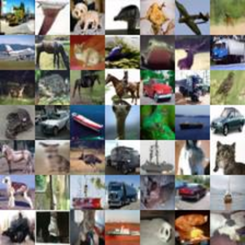
(a) Baseline

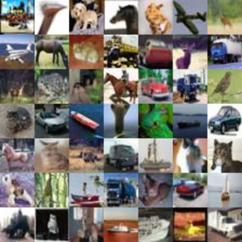
(b) Ours

Figure 5: Displayed are the generated images of baseline model and our model using DDIM with inference step of 1000. The results demonstrate our model’s superior image generation capabilities, significantly reducing the occurrence of OOD samples.

Comparison of Inference Consistency. Table 2 compares the consistency of our method with the baseline. Our approach demonstrates improved consistency at inference steps in {50, 20, 10, 5}, achieved by avoiding crossing in the inference flow. For larger steps in {1000, 100}, cross points in the inference flow have only a minor impact due to the larger steps and smaller stride. Consequently, our method and the baseline perform similarly in terms of $\operatorname{IFC}$.

Setting	Method	$\operatorname{IFC}$
DDIM-1000	iDDPM	28.58
	Ours	28.37
DDIM-100	iDDPM	29.72
	Ours	29.96
DDIM-50	iDDPM	30.85
	Ours	31.40
DDIM-20	iDDPM	33.94
	Ours	35.11
DDIM-10	iDDPM	38.51
	Ours	40.21
DDIM-5	iDDPM	46.11
	Ours	47.96

Table 2: We compare the consistency of baseline and our method. We generate 1000 samples using DDIM with inference steps in {1000, 100, 50, 20, 10, 5}.

4.3 Ablation Study

	Setting	IS	FID
Bootstrap	w/o bootstrap	5.93	79.70
	exp-schedule	9.22	5.24
	fix-prob(Ours)	9.38	4.84
Condition	$x_{0}$ condition	9.64	20.21
	mid condition	7.15	59.09
	$\hat{\epsilon}$ condition(Ours)	9.38	4.84
Network	Double Unet	9.65	6.26
	ControlNet-based(Ours)	9.38	4.84
Inference strategy	zero condition	9.06	6.43
	${\epsilon}$ condition	7.86	27.00
	$\hat{\epsilon}$ condition(Ours)	9.38	4.84

Table 3: Ablation study. We generate 10k samples using DDIM with 1000 inference step.

In this section, we verify the effectiveness of each component through ablation studies, summarized in Table 3.

Ablation of bootstrap. The impact of bootstrap strategy is evident from Table 3. We conducted experiments under three settings: without bootstrap (w/o bootstrap), exponential schedule (exp-schedule), and fixed probability (fix-probability). In the w/o bootstrap setting, $\hat{\epsilon}t=\epsilon\theta(x_{t},\mathbf{0},t)$ is consistently used. For exp-schedule, the probability of using this setting increases exponentially. The results indicate that the absence of a bootstrap strategy can significantly diminish model performance.

Ablation of condition. We then examine how different conditions affect the model. $x_{0}$ condition denotes that the model uses the predicted image as condition. Mid condition denotes that the model uses the midpoint of the training flow, i.e. $\frac{\hat{x}_{0}+\hat{\epsilon}}{2}$ as the condition. During the inference stage, each method utilizes its corresponding condition as the condition. As discussed in Sec. 3.3, the midpoint shows the poorest performance, likely because it is closest to the training flows cross point. Due to the stability of $\epsilon$, using $\hat{\epsilon}$ as a condition leads to a significant improvement of FID compared with $x_{0}$ condition.

Ablation of architecture. The study in Table 3 also investigates network effectiveness. We experimented with two different architectures, namely Double Unet and ControlNet-based. The Double Unet simply expands the input channel of the Unet model, and concatenates the input and condition along the channel. The ControlNet-based model implements conditioning similar to ControlNet [31]. Results indicate that applying ControNet can improve FID by 1.42.

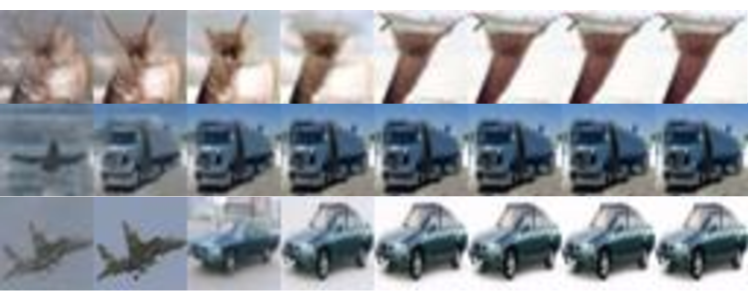
(a) unconditional

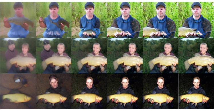
(b) class condition

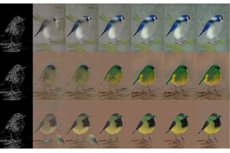
(c) canny condition

Figure 6: Here are the generated images with different conditions. (a): We generate images on Cifar-10 using iDDPM with inference step in {5, 10, 20, 50, 100, 200, 500, 1000}. (b): we generate images on ImageNet [20] using LDM [19] with inference step in {5, 10, 20, 50, 100, 500}. (c): We generate images with the canny condition using Stable Diffusion [19] with inference step in {5, 10, 20, 50, 100, 500}. We sample all images with DDIM [23].

Ablation of inference strategy. Finally, we compared different inference strategies. After training a model following Sec. 3.4, we applied various conditions during inference. The Zero condition always uses $\mathbf{0}$ as the condition. The $\epsilon$ condition uses the initial noise $\epsilon$, and the $\hat{\epsilon}$ condition utilizes the estimated noise $\hat{\epsilon}$. Due to the discrepancy between the initial noise $\epsilon$ and the estimated noise $\hat{\epsilon}$, the $\epsilon$ condition significantly reduced performance. While the Zero condition avoids ambiguity in the training stage, it leads to a slight performance decline during inference as the inference flow cannot bypass crossing and may redirect at the cross point.

4.4 Discussion

This section offers an alternative perspective to understand our Non-Cross Diffusion. The inclusion of $\hat{\epsilon}_{t}$ in the model input is seen as a strong conditional constraint, which we propose can reduce the variability of semantic information, thus lessening the severity of xFlow during inference.

Specifically, the $\hat{\epsilon}_{t}$ condition in Non-Cross Diffusion is highly specific at the pixel level, making it an exceptionally stringent constraint. Consequently, Non-Cross Diffusion effectively mitigates the xFlow issue. An interesting question arises: how would xFlow be influenced by other forms of conditions with varying degrees of strength? To investigate this, we employed the pre-trained ControlNet model for empirical analysis and results.

Fig. 6 shows generated unconditional images from iDDPM, class conditional images from ImageNet LDM [19], and Canny conditional images with ControlNet [31]. In Fig. 6(a), unconditional generation on Cifar-10 at steps {5, 10, 20, 50, 100, 200, 500, 1000} presents a significant shift in the semantic content of the images at each step: from airplane to automobile class. In contrast, Fig. 6(b) and 6(c) under the tench class and Canny edge conditions, respectively, demonstrate more consistent semantic content across steps, despite some variability in details such as the background and tail. Therefore, we hypothesize that stronger conditions ease the severity of xFlow.

5 Conclusion

In this study, we have addressed the xFlow phenomenon in diffusion models, characterized by deviations in generative flow that result in semantic inconsistencies and suboptimal image generation. Our novel approach, ‘Non-Cross Diffusion’, innovates in the realm of generative modeling by adopting ordinary differential equation models. Our empirical investigations, including both a toy example and the Cifar-10 image dataset, demonstrate the substantial efficacy of the Non-Cross Diffusion approach. The results show a marked reduction in semantic inconsistencies at various inference stages and significant improvements in the overall performance of diffusion models.

Looking Ahead. The identification of xFlow as a critical issue during inference opens new avenues for research and application optimization. Despite the effectiveness of the proposed Non-Cross Diffusion approach on mitigating xFlow, we acknowledge the challenges associated with retraining large-scale diffusion models such as Stable Diffusion. However, we are optimistic that future research will find ways to integrate these improvements into existing models, potentially circumventing the need for extensive retraining. This paper lays the groundwork for such advancements, aiming to enhance the reliability and quality of diffusion model outputs.

Supplementary Material

6 Continuity of Diffusion Models

In Section 3.3, we select the condition based on the inherent continuity in diffusion models. Continuity, although abstract, is pivotal to understanding why we select noise as the condition. To make this concept more tangible, we demonstrate it by introducing variable scale perturbations at different time steps. Specifically, for a fixed timestep $t$ and diffusion model $\epsilon_{\theta}$, the $\epsilon_{\theta}(x_{t},t)$ is continuous with respect to $x_{t}$. This implies that for any $\tilde{x}_{t}$ close to $x_{t}$, the resulting image remains similar, which shows the continuity principle in diffusion models.

6.1 Perturbation on Noise

Practically, for initial noise $\epsilon$, i.e. $t=T$, we add perturbation as follows:

$$\tilde{\epsilon}=\frac{\epsilon+w\cdot\epsilon_{p}}{\sqrt{1+w^{2}}},$$ (16)

where $\epsilon_{p}$ is a perturbation sampled from a standard Gaussian distribution and $w$ denotes the scale of perturbation. For intermediate $x_{t}$ in timestep $t$, we first estimate the noise through the baseline unconditional diffusion model:

$$\hat{\epsilon}=\epsilon_{\theta}(x_{t},t).$$ (17)

Then we add perturbation to the estimated noise $\hat{\epsilon}$:

$$\tilde{\epsilon}=\frac{\hat{\epsilon}+w\cdot\epsilon_{p}}{\sqrt{1+w^{2}}},$$ (18)

and we get the denoised image as follows:

$$x_{t-1}=\sqrt{\bar{\alpha}_{t-1}}\hat{x}_{0}+\sqrt{1-\bar{\alpha}_{t-1}}\tilde{\epsilon},$$ (19)

where $\hat{x_{0}}$ is predicted by $\hat{\epsilon}$ and $x_{t}$.

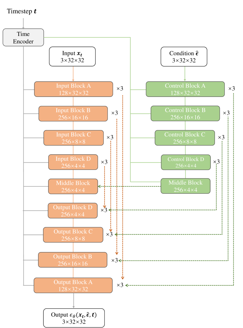
Figure 7: The architecture of our model. We show the shape on each module of its output.

6.2 Result with Perturbation

As depicted in Fig. 8, with a minimal scale, such as 0.01, there is negligible impact on the semantic content of the images across different steps. The semantic information of generated images remains intact. As the scale increases, the disparity between the original and the perturbed images becomes more pronounced. At a scale of 0.2, the semantic alterations are most notable, as exemplified by significant changes in elements like the postures of animals in the images. For instance, the positions of a cat or a deer might shift noticeably. Despite these changes, the overall semantic context — the fundamental identity of the subjects — remains unchanged, underscoring the continuity intrinsic to diffusion models.

However, at a higher scale, such as 0.5, the semantic shift becomes dramatic. The generated images undergo substantial transformations, to the extent that the class of the subject in the image can completely change, such as transitioning from a cat to a frog.

The observation shows that for the cross point, i.e. the noised images are identical, with similar conditions, the generated image will still remain the same and cannot avoid crossing. With more distinct conditions, the effectiveness of avoiding crossing increases.

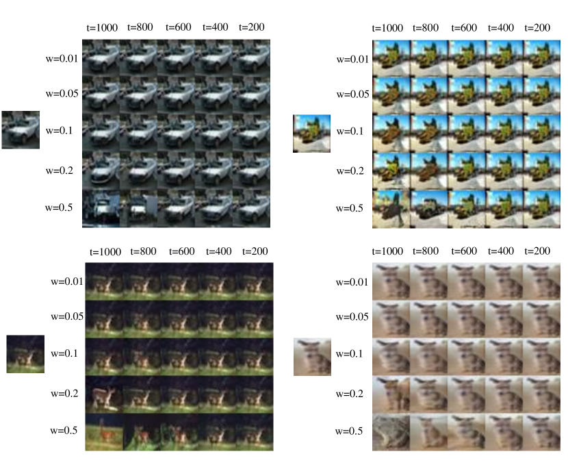
Figure 8: We sample images using iDDPM[17] with 1000 inference steps on Cifar-10. For the image grid, from left to right, the perturbation is added at $t=1000,800,600,400,200$. From top to bottom, the perturbation is added with weight $w=0.01,0.05,0.1,0.2,0.5$. We sample all images with DDIM[23]

7 Details of our model

ControlNet-based. Figure 7 presents the architecture of our proposed model. Notably, we have omitted the zero convolution layer originally found in the ControlNet [31] design. Both the UNet and Control Blocks are concurrently trained from scratch. The outputs from Control Block A, B, C, and D are integrated with the respective outputs of the input blocks. This integration is achieved by adding the outputs from the Control Blocks to those of the Input Blocks, followed by concatenation with the corresponding output from the Output Blocks. The output from the middle block of ControlNet is directly added to the output of UNet’s middle block, and then this combined output is fed into UNet’s output block D.

Double UNet in Ablation Study. For Double UNet setting in ablation study, we modified the input channel of the first layer in UNet. This modification involved doubling the input channel, i.e., changing the input channel of the first convolution layer from 3 to 6.

8 Training and Inference Algorithm

Algorithm 1 shows the training pipeline of our method. As described in Section 3, we replace the use of initial noise $\epsilon$ with predicted noise $\hat{\epsilon}$ to avoid trivial solutions and training collapse. During training, we set $\hat{\epsilon}=\mathbf{0}$, with a fixed probability $p=0.5$, and otherwise, $\hat{\epsilon}$ is assigned the value of $\epsilon_{\theta}(x_{t},\mathbf{0},t)$.

Algorithm 1 Training Stage

0:   diffusion model $\epsilon_{\theta}$, training step $T$

1:   repeat

2:      sample $x_{0}\sim q(x_{0}),\epsilon\sim\mathcal{N}(0,\mathbf{I}),t\sim\mathcal{U}(0,T-1)$

3:      compute noised image $x_{t}=\sqrt{\bar{\alpha}_{t}}x_{0}+\sqrt{1-\bar{\alpha}_{t}}\epsilon$

4:      sample $p\sim U(0,1)$

5:      $\hat{\epsilon}\leftarrow\mathbf{0}$

6:      if $p\geq 0.5$ then

7:         $\hat{\epsilon},\hat{x}_{0}\leftarrow\epsilon_{\theta}(x_{t},\hat{\epsilon},t)$

8:         $\hat{\epsilon}\leftarrow stop\_gradient(\hat{\epsilon})$

9:      end if

10:      $\hat{\epsilon},\hat{x}_{0}\leftarrow\epsilon_{\theta}(x_{t},\hat{\epsilon},t)$

11:      $Loss=MSE(\epsilon,\hat{\epsilon})$

12:   until converged

Algorithm 2 shows the inference pipeline of our method. We use estimated noise in the previous step instead of the current step as the condition and iteratively predict $\hat{\epsilon}$, which can effectivly alleviate the computational costs.

Algorithm 2 Inference Stage

0:   diffusion model $\epsilon_{\theta}$, inference step $T$

1:   sample $x\sim\mathcal{N}(0,\mathbf{I})$

2:   $\hat{\epsilon}\leftarrow\mathbf{0}$

3:   for $t$ in $range(T,0)$ do

4:      $\hat{\epsilon},\hat{x}_{0}\leftarrow\epsilon_{\theta}(x,\hat{\epsilon},t)$

5:      $x=\sqrt{\bar{\alpha}_{t-1}}\hat{x}_{0}+\sqrt{1-\bar{\alpha}_{t-1}}\hat{\epsilon}$

6:   end for

7:   return generated image $x$

References

- Avrahami et al. [2022] Omri Avrahami, Dani Lischinski, and Ohad Fried. Blended diffusion for text-driven editing of natural images. In Proceedings of the IEEE/CVF Conference on Computer Vision and Pattern Recognition (CVPR), pages 18208–18218, 2022.
- Brooks et al. [2023] Tim Brooks, Aleksander Holynski, and Alexei A. Efros. Instructpix2pix: Learning to follow image editing instructions. In Proceedings of the IEEE/CVF Conference on Computer Vision and Pattern Recognition (CVPR), pages 18392–18402, 2023.
- Chen et al. [2022] Ting Chen, Ruixiang Zhang, and Geoffrey Hinton. Analog bits: Generating discrete data using diffusion models with self-conditioning. arXiv preprint arXiv:2208.04202, 2022.
- Dhariwal and Nichol [2021] Prafulla Dhariwal and Alexander Nichol. Diffusion models beat gans on image synthesis. Advances in neural information processing systems, 34:8780–8794, 2021.
- Fan and Lee [2023] Ying Fan and Kangwook Lee. Optimizing ddpm sampling with shortcut fine-tuning. arXiv preprint arXiv:2301.13362, 2023.
- Gao et al. [2023a] Ruiyuan Gao, Kai Chen, Enze Xie, Lanqing Hong, Zhenguo Li, Dit-Yan Yeung, and Qiang Xu. Magicdrive: Street view generation with diverse 3d geometry control. arXiv preprint arXiv:2310.02601, 2023a.
- Gao et al. [2023b] Ruiyuan Gao, Chenchen Zhao, Lanqing Hong, and Qiang Xu. Diffguard: Semantic mismatch-guided out-of-distribution detection using pre-trained diffusion models. In Proceedings of the IEEE/CVF International Conference on Computer Vision, pages 1579–1589, 2023b.
- Goodfellow et al. [2014] Ian Goodfellow, Jean Pouget-Abadie, Mehdi Mirza, Bing Xu, David Warde-Farley, Sherjil Ozair, Aaron Courville, and Yoshua Bengio. Generative adversarial nets. Advances in neural information processing systems, 27, 2014.
- Heusel et al. [2017] Martin Heusel, Hubert Ramsauer, Thomas Unterthiner, Bernhard Nessler, and Sepp Hochreiter. Gans trained by a two time-scale update rule converge to a local nash equilibrium. Advances in neural information processing systems, 30, 2017.
- Ho and Salimans [2022] Jonathan Ho and Tim Salimans. Classifier-free diffusion guidance. arXiv preprint arXiv:2207.12598, 2022.
- Ho et al. [2020] Jonathan Ho, Ajay Jain, and Pieter Abbeel. Denoising diffusion probabilistic models. Advances in neural information processing systems, 33:6840–6851, 2020.
- Karras et al. [2022] Tero Karras, Miika Aittala, Timo Aila, and Samuli Laine. Elucidating the design space of diffusion-based generative models. Advances in Neural Information Processing Systems, 35:26565–26577, 2022.
- Krizhevsky et al. [2009] Alex Krizhevsky, Geoffrey Hinton, et al. Learning multiple layers of features from tiny images. Tech Report, 2009.
- Liu et al. [2022] Xingchao Liu, Chengyue Gong, and Qiang Liu. Flow straight and fast: Learning to generate and transfer data with rectified flow. arXiv preprint arXiv:2209.03003, 2022.
- Lu et al. [2022] Cheng Lu, Yuhao Zhou, Fan Bao, Jianfei Chen, Chongxuan Li, and Jun Zhu. Dpm-solver: A fast ode solver for diffusion probabilistic model sampling in around 10 steps. Advances in Neural Information Processing Systems, 35:5775–5787, 2022.
- Nichol et al. [2022] Alex Nichol, Prafulla Dhariwal, Aditya Ramesh, Pranav Shyam, Pamela Mishkin, Bob McGrew, Ilya Sutskever, and Mark Chen. Glide: Towards photorealistic image generation and editing with text-guided diffusion models, 2022.
- Nichol and Dhariwal [2021] Alexander Quinn Nichol and Prafulla Dhariwal. Improved denoising diffusion probabilistic models. In International Conference on Machine Learning, pages 8162–8171. PMLR, 2021.
- Ramesh et al. [2022] Aditya Ramesh, Prafulla Dhariwal, Alex Nichol, Casey Chu, and Mark Chen. Hierarchical text-conditional image generation with clip latents, 2022.
- Rombach et al. [2022] Robin Rombach, Andreas Blattmann, Dominik Lorenz, Patrick Esser, and Björn Ommer. High-resolution image synthesis with latent diffusion models. In Proceedings of the IEEE/CVF conference on computer vision and pattern recognition, pages 10684–10695, 2022.
- Russakovsky et al. [2015] Olga Russakovsky, Jia Deng, Hao Su, Jonathan Krause, Sanjeev Satheesh, Sean Ma, Zhiheng Huang, Andrej Karpathy, Aditya Khosla, Michael Bernstein, Alexander C. Berg, and Li Fei-Fei. ImageNet Large Scale Visual Recognition Challenge. International Journal of Computer Vision (IJCV), 115(3):211–252, 2015.
- Saharia et al. [2022] Chitwan Saharia, William Chan, Saurabh Saxena, Lala Li, Jay Whang, Emily L Denton, Kamyar Ghasemipour, Raphael Gontijo Lopes, Burcu Karagol Ayan, Tim Salimans, Jonathan Ho, David J Fleet, and Mohammad Norouzi. Photorealistic text-to-image diffusion models with deep language understanding. In Advances in Neural Information Processing Systems, pages 36479–36494. Curran Associates, Inc., 2022.
- Salimans et al. [2016] Tim Salimans, Ian Goodfellow, Wojciech Zaremba, Vicki Cheung, Alec Radford, and Xi Chen. Improved techniques for training gans. Advances in neural information processing systems, 29, 2016.
- Song et al. [2020a] Jiaming Song, Chenlin Meng, and Stefano Ermon. Denoising diffusion implicit models. arXiv preprint arXiv:2010.02502, 2020a.
- Song and Ermon [2019] Yang Song and Stefano Ermon. Generative modeling by estimating gradients of the data distribution. Advances in neural information processing systems, 32, 2019.
- Song et al. [2020b] Yang Song, Jascha Sohl-Dickstein, Diederik P Kingma, Abhishek Kumar, Stefano Ermon, and Ben Poole. Score-based generative modeling through stochastic differential equations. arXiv preprint arXiv:2011.13456, 2020b.
- Tumanyan et al. [2023] Narek Tumanyan, Michal Geyer, Shai Bagon, and Tali Dekel. Plug-and-play diffusion features for text-driven image-to-image translation. In Proceedings of the IEEE/CVF Conference on Computer Vision and Pattern Recognition (CVPR), pages 1921–1930, 2023.
- Vahdat and Kautz [2020] Arash Vahdat and Jan Kautz. Nvae: A deep hierarchical variational autoencoder. Advances in neural information processing systems, 33:19667–19679, 2020.
- Yang et al. [2022a] Yijun Yang, Ruiyuan Gao, Yu Li, Qiuxia Lai, and Qiang Xu. What you see is not what the network infers: detecting adversarial examples based on semantic contradiction. arXiv preprint arXiv:2201.09650, 2022a.
- Yang et al. [2022b] Yijun Yang, Ruiyuan Gao, and Qiang Xu. Out-of-distribution detection with semantic mismatch under masking. In European Conference on Computer Vision, pages 373–390. Springer, 2022b.
- Yoon et al. [2023] TaeHo Yoon, Kibeom Myoung, Keon Lee, Jaewoong Cho, Albert No, and Ernest K Ryu. Censored sampling of diffusion models using 3 minutes of human feedback. arXiv preprint arXiv:2307.02770, 2023.
- Zhang et al. [2023] Lvmin Zhang, Anyi Rao, and Maneesh Agrawala. Adding conditional control to text-to-image diffusion models. In Proceedings of the IEEE/CVF International Conference on Computer Vision, pages 3836–3847, 2023.