Extrapolatable Transformer Pre-training for Ultra Long Time-Series Forecasting

Abstract.

Large-scale pre-trained models (PTMs) such as BERT and GPT have recently achieved great success in Natural Language Processing and Computer Vision domains. However, the development of PTMs on time-series data is lagging behind. This underscores the limitations of the existing transformer-based architectures, particularly their scalability to handle large-scale data and ability to capture long-term temporal dependencies. In this study, we present Timely Generative Pre-trained Transformer (TimelyGPT). TimelyGPT employs an extrapolatable position (xPos) embedding to encode trend and periodic patterns into time-series representations. It also integrates recurrent attention and temporal convolution modules to effectively capture global-local temporal dependencies. Our experiments show that TimelyGPT excels in modeling continuously monitored biosignals and irregularly-sampled time series data commonly observed in longitudinal electronic health records (EHRs). In ultra-long-term forecasting experiment, TimelyGPT achieves accurate extrapolation up to 6,000 timesteps of body temperature during the sleep stage transition given a short look-up window (i.e., prompt) containing only 2,000 timesteps. We further demonstrated TimelyGPT ’s forecasting capabilities on a preprocessed longitudinal healthcare administrative database called PopHR consisting of 489,000 patients randomly sampled from Montreal population. Together, we envision TimelyGPT to be useful in a broad spectrum of health domains including long-term patient health state forecasting and patient risk trajectory prediction.

1. Introduction

Time-series forecasting holds significant importance in healthcare, given its potential to trace patient health trajectories and predict medical outcomes (Ma et al., 2023; Eldele et al., 2021; Fawaz et al., 2019). In the field of healthcare, there are two primary categories: continuous and irregularly-sampled time-series data. Continuous time-series, such as biosignals, has been extensively studied in various applications including health monitoring (Stirling et al., 2020), disease classification (Phan et al., 2021), and physical activity prediction (Reiss et al., 2019b). Irregularly-sampled time series is commonly found in clinical records, where spontaneous updates are made due to the outpatient hospital visits or inpatient hospital stays (Zhang et al., 2022a). The key challenge is to extract meaningful representations from these time-series to make accurate long-term forecasting. A promising approach is to adopt transfer learning (Ma et al., 2023). Initially, a model is pre-trained on large-scale datasets to learn the contextualized temporal representations. This pre-trained model (PTM) is then fine-tuned to forecast target sequences or predict target labels.

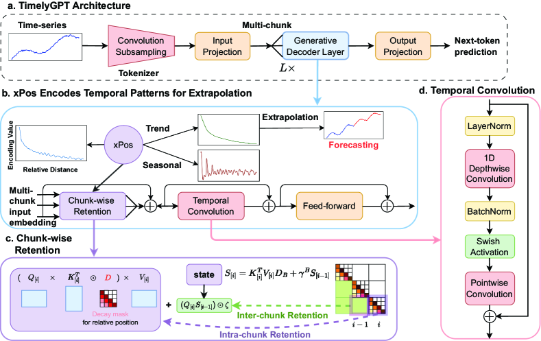
Figure 1. TimelyGPT overview. a. TimelyGPT  consists of a convolution-subsampling tokenizer followed by $L$ decoder layers, with detailed overflow provided in Appendix B.3. b. Each decoder layer is coupled with extrapolatable position embedding (Section. 3.1) that encodes trend and periodic patterns into representations, facilitating forecasting with extrapolation ability. c. Chunk-wise Retention. (Section 3.2) consists of parallel intra-chunk Retention and recurrent inter-chunk Retention, effectively handling long sequences. d. Temporal Convolution (Section 3.3) captures nuanced local interactions from time-series representations.

The recent impressive achievements of Transformer PTMs in Natural Language Processing (NLP) and Computer Vision (CV) domains have inspired growing interest in time-series Transformer PTMs. Time-Series Transformer (TST) uses a mask-and-reconstruction pre-training strategy to extract contextualized representations from time series (Zerveas et al., 2020). Cross-Reconstruction Transformer (CRT) learns temporal representations by dropping and reconstructing certain segments (Zhang et al., 2023). Additionally, Transformer PTMs have been applied to traffic (Zhao et al., 2022), tabular (Padhi et al., 2021), and speech time-series (Liu et al., 2020, 2021).

Transfer learning by pre-training on large time-series data followed by fine-tuning for long-term time series forecasting (LTSF) tasks is a promising avenue. However, existing studies primarily focus on training from scratch on limited data for LTSF or classification tasks (Ma et al., 2023). These studies often introduce tailored architectures and attention modules to extract complex temporal dependencies (Zhou et al., 2021; Wu et al., 2022; Zhou et al., 2022). However, the scalability of these transformers on large datasets remains untested (Kaplan et al., 2020). Additionally, recent studies question Transformer’s benefits in LTSF, suggesting they may not outperform linear models (Zeng et al., 2022). They argue that permutation-invariant nature of self-attention causes the loss of temporal information. Transformers often underperform compared to convolution-based models, potentially due to their struggles with local features and multi-scale features (Yue et al., 2022; Tang et al., 2021). Overall, existing research on time-series transformers often lacks rigorous evaluation on large datasets and does not consistently outperform conventional approaches on small data. This underscores the need to tailor transformer architectures for time-series applications.

In this study, we provide an in-depth analysis of existing time-series transformers, covering key aspects such as the attention mechanism, position embedding, and extrapolation. We argue that the seemingly inadequacy of current transformer-based models in modeling time-series data is due to their inability to model large-scale time series. Once these challenges are resolved, we would observe a typical scaling law found in NLP and CV domains (Kaplan et al., 2020; Zhai et al., 2022). Inspired by our insights, we introduce Timely Generative Pre-trained Transformer (TimelyGPT) (Fig. 1) that utilizes an extrapolatable position (xPos) embedding to encode trend and periodic patterns into time-series representations (Sun et al., 2022). TimelyGPT integrates recurrent attention (also known as Retention) and convolution modules for effectively capturing both global temporal dependencies and nuanced local interactions (Sun et al., 2023; Gulati et al., 2020).

We emphasize the benefits of pre-training on large-scale time-series biosignals and longitudinal EHR data and then fine-tuning on specific tasks. Experimental results reveal that TimelyGPT effectively extrapolates temporal representations for ultra-long-term forecasting. The key contributions of our research are threefold:

1. We employ extrapolatable xPos embedding (Fig. 1b) to encode both trend and periodic patterns into time-series representations, facilitating ultra-long-term forecasting.

2. We extend recurrent attention (Fig. 1c) to handle both continuous and irregularly-sampled time-series data;

3. We introduce convolution subsampling tokenizer (Fig. 1a) to extract features from raw time-series and temporal convolution (Fig. 1d) to sift local features among the timesteps.

Table 1. The model parameters and utilized datasets of time-series transformers and comparison methods. These setups are sourced from papers and default implementation. Over-parameterization indicates model parameters $>>$ dataset size (timestep).

Method	Application	Dimension	Layer	Model Parameter	Dataset Size (Timestep)	Param versus Data
Informer	Forecasting	512	3	11.3M	69.7K	Over-param
Autoformer	Forecasting	512	3	10.5M	69.7K	Over-param
Fedformer (F/W)	Forecasting	512	3	16.3/114.3M	69.7K	Over-param
PatchTST	Forecasting	128	3	1.2M	69.7K	Over-param
DLinear	Forecasting	-	1	70K	69.7K	Adequate
Conformer (L)	Classification	512	18	118.8M	55.9B	Adequate
CRT	Pre-training	128	18	8.8 M	109.2M	Adequate

2. Related work

2.1. Transformer Scaling Law in Time-Series

Despite the broad applications of transformer-based models in time-series data such as speech (Gulati et al., 2020; Radford et al., 2022), biosignals (Song et al., 2023), and traffic flow (Shao et al., 2022; Jiang et al., 2023), their effectiveness in capturing temporal dependencies in LTSF task has been limited and often underperforms compared to linear models (Zeng et al., 2022). As Table 1 indicates, time-series transformer models often have much more parameters than the dataset size (timestep) with only two exceptions, namely large-size Conformer and CRT. Such disparities imply that many transformers may be over-parameterized, leading to highly variable performance. In Section 4.2, our study validates the Transformer scaling law in time-series domain (i.e., scaling up both model parameters and dataset size to improve performance) (Kaplan et al., 2020; Zhai et al., 2022). For all benchmark experiments, our proposed TimelyGPT effectively pre-trains on large-scale data with model parameters aligned to this scaling law.

2.2. Self-attention Module

As one of the prominent time-series transformers, Conformer utilizes the self-attention mechanism to capture long-range global contexts in speech data (Gulati et al., 2020). When combined with convolution modules, Conformer enhances self-attention mechanism by exploiting fine-grained local patterns. Although widely successful, its quadratic complexity has spurred exploration of attention-free modules such as Multi-Layer Perceptron (MLP) (Tolstikhin et al., 2021), implicit long convolution (Poli et al., 2023), and Recurrent Neural Network (RNN) (Peng et al., 2023; Sun et al., 2023). In particular, RNN-based attention modules have scaled up to 14 billion parameters while maintaining competitive performance with linear training and constant inference complexities. These modules are particularly well-suited for time-series modeling by effectively capturing sequential dependencies (Gu et al., 2022). In this study, TimelyGPT integrates Retention mechanism and convolution modules to effectively capture both global and local contexts.

2.3. Relative Position Embedding

The absolute position embedding is inadequate in capturing temporal relations (Zeng et al., 2022). While the sinusoidal function utilizes discrete position index, it struggles with encoding positional information into continuous timescale, such as trend and periodic patterns in time-series. In contrast, speech transformers leverage the relative position embedding of T-5 model to handle continuous time (Gulati et al., 2020; Kim et al., 2022), addressing the shortcomings of absolute position embedding(Deihim et al., 2023). Rotary Position Embedding (RoPE), prevalent in numerous large language models (Brown et al., 2020; Touvron et al., 2023; Penedo et al., 2023), applies rotation matrices to encode time information from relative distances (Su et al., 2022). Additionally, RNN-based transformer RWKV uses exponential decay to encode time information based on relative distance (Peng et al., 2023). Bridging these techniques, xPos embedding utilizes both rotation and exponential decay to effectively capture long-term dependencies (Sun et al., 2022). We provide details of these embedding methods in Appendix B.1.

In time-series domain, xPos embedding effectively encodes both trend and periodic patterns for modeling crucial features from healthcare data. For continuous biosignals, trend patterns including body temperature and vital signs are important indicators of health. The electrocardiogram (ECG) that measures the body’s physiological rhythms also exhibits periodic patterns. For irregularly-sampled time series, the age-related susceptibility to illnesses is observed in longitudinal population studies from EHRs (Ahuja et al., 2022; Song et al., 2022). EHRs also exhibit periodic patterns, especially for chronic diseases like COPD with alternating exacerbation and medical treatment effects. We hypothesize that xPos emebdding can encode trend and periodic patterns into the token embedding, enhancing both performance and interpretability in healthcare time-series applications.

2.4. Extrapolating Attention with xPos

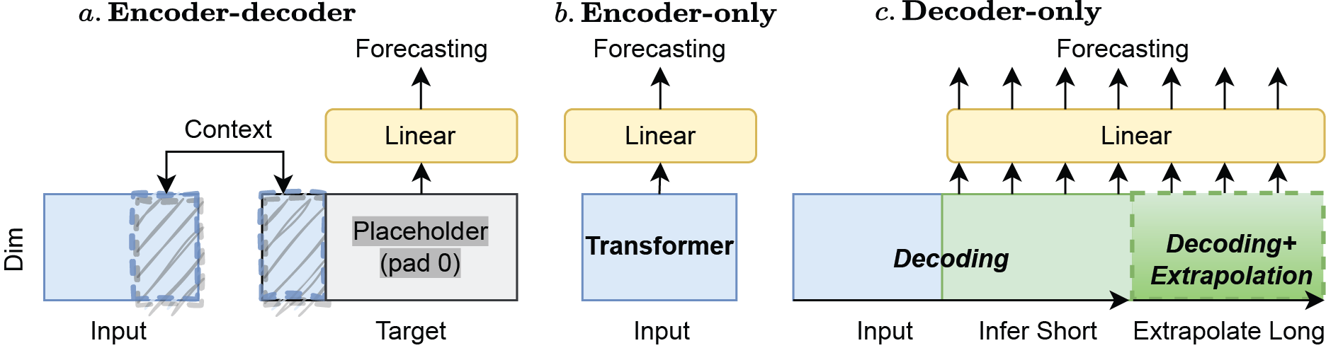
Figure 6. Forecasting transformer architectures. a. The encoder-decoder architecture employs a one-forward prediction without autoregressive decoding for forecasting. b. The encoder-only architecture directly projects the input representation to make forecasting. c. The proposed decoder-only architecture in TimelyGPT decodes embedding for future timesteps autoregressively and utilizes extrapolation technique for foresting unseens timesteps for sequence longer than any of training sequences.

Existing studies on forecasting transformers have mainly focused on encoder-decoder architectures (Fig. 6a) (Zhou et al., 2021). The input to the decoder is the concatenation of input sequence and a placeholder for the target sequence (i.e., zero padding) of a fixed length. Instead of predicting the outputs autoregressively, these models forecast all timesteps at once (Zeng et al., 2022). Similarly, encoder-only models leverage encoded embedding for forecasting with the help of a linear layer (Fig. 6b) (Nie et al., 2023). While these works attribute the poor performance to the autoregressive decoding (Zhou et al., 2021), recent studies suggest that it may be due to the difficulty of Transformer in representing unseen positions, known as the challenge of extrapolation (Press et al., 2022). In particular, transformer performance rapidly declines as it starts to forecast sequence longer than any of the training sequences (Press et al., 2022). Indeed, both encoder-decoder and encoder-only transformers lack extrapolation ability and rely heavily on their linear layer for forecasting (Li et al., 2023), limiting their effectiveness in LTSF tasks.

The challenge in extrapolation lies in the difficulty of generalizing position embedding to unseen positions. To address this issue, the Attention with Linear Biases (ALiBi) adjusts attention with a penalty linearly correlated with token distances (Press et al., 2022). Building on this, xPos embedding employs exponential decay, assigning penalties based on relative distances (Sun et al., 2022). Consequently, xPos can handle inference length up to eight times the training length, while still maintaining comparable performance. Our TimelyGPT extends xPos from NLP domain to ultra-long-term forecasting in time-series domain, focusing on exploring the underlying mechanisms that enable the temporal extrapolation.

3. TimelyGPT Methodology

Our proposed TimelyGPT effectively pre-trains on unlabeled data using next-token prediction task to learn temporal representations (Fig. 1a). It first processes time-series inputs using a convolution-subsampling tokenizer for token embedding (Section 3.3). To further extract temporal pattern, TimelyGPT integrates three technical contributions. First, TimelyGPT utilizes extrapolatable xPos embedding to encode trend and periodic patterns for extrapolation (Fig. 1b, Section 3.1). Second, TimelyGPT utilizes Retention module to capture global content (Fig. 1c, Section 3.2). Third, TimelyGPT deploys convolution module to capture the local content (Fig. 1d, Section 3.3). The integration of Retention and Convolution modules enable learning the interactions between global and local content.

3.1. Extrapolatable Position Embedding Encodes Temporal Patterns

Position embedding is crucial for Transformer, as the self-attention mechanism does not inherently discern token order. Typically, time-series transformer models adopt absolute position embedding that is directly added to the token embedding. In contrast, xPos encodes relative position information into token embedding based on the distance $n-m$ between two tokens $n$ and $m$ (Sun et al., 2022). Given an input embedding ${\bm{X}}\in\mathbb{R}^{N\times d}$, where $N$ is number of tokens and $d$ is hidden dimension, xPos is integrated into the $n$-th token embedding through rotation matrix $e^{i\theta n}$ and exponential decay $\gamma^{n}$:

$$\tilde{\bm{Q}}_{n}\tilde{\bm{K}}_{m}={\bm{X}}_{n}{\bm{W}}_{Q}(\gamma e^{i\theta})^{n-m}{\bm{X}}_{m}{\bm{W}}_{K}=\gamma^{n-m}\hat{\bm{Q}}_{n}\hat{\bm{K}}_{m}$$

(1) $$\hat{\bm{Q}}_{n}={\bm{X}}_{n}{\bm{W}}_{Q}e^{i\theta n},\,\hat{\bm{K}}_{m}={\bm{X}}_{m}{\bm{W}}_{K}e^{-i\theta m}$$

where $\theta$ and $\gamma$ indicate position-dependent rotation and decay hyperparameters (Su et al., 2022; Sun et al., 2022). The exponential decay $\gamma^{n-m}$ effectively attenuates the influence of distant tokens, aiding in capturing long-term dependency and extrapolation ability (Sun et al., 2022).

While originally designed for language modeling, xPos provides a compelling way for time-series modeling, mirroring the seasonal-trend decomposition (Fig. 1c). Its exponential decay $\gamma^{n-m}$ naturally concentrates on recent time while diminishing the influence of distant time, reflecting the trend momentum of time-series. The rotation matrix $e^{i\theta(n-m)}$ captures the seasonal component of the time-series data through the sinusoidal oscillations. As our first contribution, this structure allows xPos-based models to encode inherent temporal patterns into token embedding for time-series modeling. TimelyGPT harnesses xPos to effectively model long-term dependencies essential for time-series forecasting. We also explore the underlying mechanisms driving the temporal extrapolation for forecasting beyond training length.

3.2. Retention for Continuous and Irregularly-sampled Time Series

We adapt the Retention mechanism to effectively handle continuous time-series data (Sun et al., 2023). The Retention mechanism based on xPos can be reformulated as an RNN to naturally model time-series data. Given the xPos embedding in Eq 3.1, the forward-pass of the Retention mechanism can be computed in parallel over all tokens:

$$\hat{\bm{Q}}_{n}={\bm{X}}_{n}{\bm{W}}_{Q}e^{i\theta n},\>\hat{\bm{K}}_{m}={\bm{X}}_{m}{\bm{W}}_{K}e^{-i\theta m},\>{\bm{V}}={\bm{X}}{\bm{W}}_{V}$$

(2) $$\text{Ret}({\bm{X}})=(\hat{\bm{Q}}\hat{\bm{K}}^{\top}\odot{\bm{D}}){\bm{V}},\>{\bm{D}}_{nm}=\begin{cases}\gamma^{n-m},&n\geq m\\ 0,&n<m\end{cases}$$

where the decay matrix ${\bm{D}}\in R^{N\times N}$ and rotation matrix $e^{i\theta(n-m)}$ encode trends and periodic patterns into the token embedding with respect to each relative distances $n-m$. When reformulated as a RNN, the Retention in Eq. 3.2 can be manifested in a recurrent forward-pass with a constant inference complexity. This reformulated RNN excels in capturing sequential dependencies from the time-series. To handle long sequences, we use chunk-wise Retention by segmenting the sequence into multiple, non-overlapped chunks (Fig. 1c). Consequently, chunk-wise Retention maintains a linear complexity for long sequences. We provide details about the three Retention forward-passes in Appendix B.2.

As our second contribution, we modify the Retention mechanism to accommodate irregularly-sampled time series, comprising $N$ samples $\{s_{1},\ldots,s_{N}\}$. Each sample $s_{n}$ is represented as a tuple $(x_{n},t_{n})$, consisting of an observation $x_{n}$ and a timestep $t_{n}$. For example, a patient’s medical history with sporadic diagnoses can be represented as an irregularly-sampled timeseries with varied time intervals. This non-uniform intervals pose challenge to traditional time-series methodologies designed for equally spaced data. To handle irregular observations, we modify the decay matrix ${\bm{D}}$ in the parallel forward-pass of Retention to accommodate the varying gaps between observations. Given two samples $s_{n}$ and $s_{m}$, the decay mask ${\bm{D}}$ is adapted according to the time gap $\Delta t_{n,m}=t_{n}-t_{m}$:

(3) $$\text{Ret}({\bm{X}})=({\bm{Q}}{\bm{K}}^{\top}\odot{\bm{D}}){\bm{V}},\;{\bm{D}}_{nm}=\begin{cases}\gamma^{\Delta t_{n,m}},&t_{r_{n}}\geq t_{r_{m}}\\ 0,&t_{r_{n}}<t_{r_{m}}\end{cases}$$

By integrating $\Delta t$ with the state variable ${\bm{S}}\in R^{d\times d}$, we adapt the recurrent forward-pass with a constant inference complexity:

$$\text{Ret}(X_{n})={\bm{Q}}_{n}{\bm{S}}_{m}=\sum_{m=1}^{n}\gamma^{\Delta t_{n,m}}{\bm{Q}}_{n}{\bm{K}}_{m}^{\top}{\bm{V}}_{m}$$

(4) $${\bm{S}}_{n}=\gamma^{\Delta{t}_{n,n-1}}{\bm{S}}_{n-1}+{\bm{K}}_{n}^{\top}{\bm{V}}_{n}$$

Given the irregular timestep $n\in\{1,\dots,B\}$ within a chunk size of $B$, we adapt a chunk-wise forward-pass with linear complexity:

$${\bm{Q}}_{[i]}={\bm{Q}}_{B_{i}:B_{i+1}},\>{\bm{K}}_{[i]}={\bm{K}}_{B_{i}:B_{i+1}},\>{\bm{V}}_{[i]}={\bm{V}}_{B_{i}:B_{i+1}}$$

$$\text{Ret}(X_{[i]})=\underbrace{({\bm{Q}}_{[i]}{\bm{K}}_{[i]}^{\top}\odot{\bm{D}}){\bm{V}}_{[i]}}_{\text{Intra-chunk}}+\underbrace{({\bm{Q}}_{[i]}{\bm{S}}_{[i-1]})\odot\zeta}_{\text{Inter-chunk}}$$

(5) $${\bm{S}}_{[i]}=\underbrace{{\bm{K}}_{[i]}^{\top}{\bm{V}}_{[i]}\odot{\bm{D}}_{B}}_{\text{Current chunk}}+\underbrace{\gamma^{B}{\bm{S}}_{[i-1]}}_{\text{Past chunk}}\quad\text{with }\zeta_{n}=\gamma^{n}$$

where $i$ indicates the chunk index, and ${\bm{D}}$ is the decay matrix with chunk size $B$ and ${\bm{D}}_{B}$ is the last row of ${\bm{D}}$.

To forecast irregularly-sampled time series, we consider two recurrent inference strategies (Eq 3.2): trajectory-based inference and time-specific inference. Both strategies make predictions based on a look-up window. The trajectory-based inference autoregressively predicts a trajectory at equal time intervals. The time-specific inference makes prediction at a specific time point. For each sample $s_{n}=(x_{n},t_{n})$, the model utilizes both the timestep $t_{n}$ and the preceding sample $s_{n-1}=(x_{n-1},t_{n-1})$ to predict its observation $x_{n}$ taking into account the time gap $\Delta t_{n,n-1}=t_{n}-t_{n-1}$.

3.3. Convolution Modules for Local Interaction

Convolution methods excel at identifying localized interactions from time-series (LeCun and Bengio, 1998). As the first part of our third contribution, we propose using a convolution-subsampling tokenizer for feature extraction from the raw time-series input (Fig. 1a). As shown in Appendix B.3, it uses multiple 1-D convolution layers to condense the time dimension and extract local features of the time-series. The convolution-subsampling tokenizer consists of two 1-D convolution with kernel size 3 and stride 2, reducing the sequence length to 1/4. Unlike the prevalent patching technique, which merely segments adjacent timesteps and features (Nie et al., 2023), convolution tokenizer effectively captures local temporal interactions.

As the second part of our third contribution, we propose a temporal convolution module using a depth-wise separable convolution (Chollet, 2017), sifting local temporal features from the time-series representations. As shown in Fig. 1d, this module starts with a layer normalization, followed by a 1-D depth-wise convolution and a point-wise convolution layers, with batch normalization and swish activation after the depth-wise convolution. The intergration of convolution and attention allows TimelyGPT to extract global-local feature interactions (Wu et al., 2020; Gulati et al., 2020). By stacking multiple decoder layers, each with a convolution module, TimelyGPT discerns multi-scale features that characterize patterns across varying time scales (Tang et al., 2021).

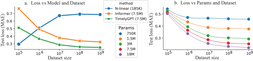
Figure 2. a. Forecasting performance of transformers increases with more data. b. TimelyGPT with more parameters tends to exhibit better performance when trained on larger datasets.

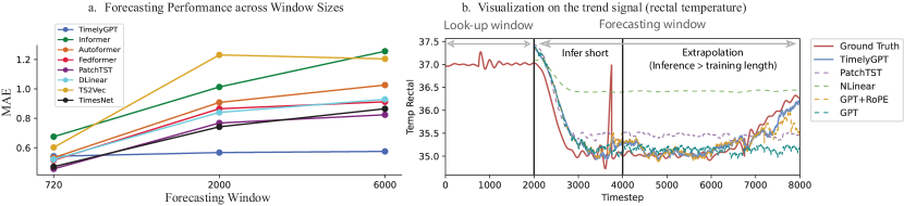
Figure 3. a. Ultra-long-term forecasting performance of 8 methods for 3 forecasting windows, with full results summarized in Table 7. b. Case analysis and visualization of a trend signal given a 2K look-up window and 6K forecasting window.

3.4. TimelyGPT for Time-Series Pre-training

In summarizing TimelyGPT’s strengths in time-series representation learning, we highlight its three key components: extrapolatable xPos embedding, Retention mechanism, and temporal convolution module. The xPos embedding encodes both trend and periodic patterns into time-series representations. Moreover, xPos effectively models long-term trend patterns, enhancing extrapolation in time-series forecasting tasks (Sun et al., 2022). The Retention mechanism, reformulated as an RNN, inherently captures sequential dependencies from time-series data (Gu et al., 2022). To effectively handle long sequences, we utilize the chunk-wise Retention with a linear complexity. The temporal convolution module, through multiple decoder layers, excels at extracting both local features and multi-scale (LeCun and Bengio, 1998; Tang et al., 2021). When combined with attention mechanisms, the convolution enables TimelyGPT to effectively learn global-local feature interactions(Gulati et al., 2020).

During per-training, TimelyGPT utilizes a Next-Token Prediction task to learn temporal representations from unlabeled data. Given a sequence with a [SOS] token, TimelyGPT predicts the subsequent tokens by shifting the sequence rightwards. At the last layer, each token’s output representation is fed into a linear layer for next-token prediction. The pre-training loss is mean squared error (MSE) for continuous signals (e.g., biosignal) or cross-entropy for discrete signals (e.g., diagnosis codes). For fine-tuning on downstream tasks, we use average pooled representations from the last layer.

4. Benchmark Experiment

4.1. Experiment Setups

We first validate the neural scaling law of transformer models, determining optimal number of model parameters for different dataset sizes (Section 4.2). We then explored TimelyGPT’s extrapolation capabilities for ultra-long-term forecasting up to 6K timesteps (Section 4.3) and analyzed extrapolation’s underlying mechanism through visualization (Section 4.4). Our evaluation extended forecasting to irregularly-sampled time series (Section 4.5). For discriminative tasks, we assessed TimelyGPT in classification and regression tasks for continuous biosignals (Section 4.6). The classification tasks was also conducted on irregularly-sampled time series (Section 4.5). Furthermore, we provided ablation studies to evaluate the contributions of various components (Section 4.8).

Datasets

For continuous time-series, we used three publicly available, large-scale datasets for pre-training: (1) the Sleep-EDF dataset with 7 types of biosignals across 1.2 billion timesteps (Kemp et al., 2000); (2) the PTB-XL dataset with 12 variates of electrocardiogram data totaling 109 million timesteps (Alday et al., 2020); (3) the PPG-Dalia dataset with 4 variates of photoplethysmograph data from 16.6 million timesteps (Reiss et al., 2019a). Additionally, we employed five other datasets for downstream discriminative tasks, namely Epilepsy (Andrzejak et al., 2001), EMG (Goldberger et al., 2000), RR, HR, SpO2 (Tan et al., 2021). For irregularly-sampled time series, we utilized a large-scale Population Health Record (PopHR) database, which was established to monitor population health in Montreal, Quebec, Canada (Shaban-Nejad et al., 2016; Yuan et al., 2018). The administrative data consist of the medical histories of 1.2 million patients in the form of International Classification of Diseases (ICD) codes. We provide dataset description and statistics in Appendix C.1, as well as data pre-processing in Appendix C.2.

Pre-training and Fine-tuning

TimelyGPT performed pre-training with Next-Token Prediction task in the last layer. For fine-tuning, we used the average-pooled output of all tokens from the last layer as the sequence representation. PatchTST adopted a masking-based approach, masking 40% of its patches as zero (Nie et al., 2023). CRT utilized a dropping-based pre-training, discarding up to 70% of patches (Zhang et al., 2023). For transformers without pre-training methods, we used a masking-based method by randomly masking 40% of timesteps (Zerveas et al., 2020). All transformers performed 20 epochs of pre-training with MSE loss, followed by 5 epochs of end-to-end fine-tuning.

4.2. Transformer’s Scalability in Time-series

We assessed the scalability of TimelyGPT, Informer (Zhou et al., 2021), and DLinear baseline (Zeng et al., 2022) on a large-scale Sleep-EDF dataset (Kemp et al., 2000). We selected datasets with timesteps ranging from $10^{5}$ to $10^{9}$, splitting each dataset into training (80%), validation (10%), and testing (10%) sets. We set the look-up and forecasting windows 256 timesteps.

Transformers with fixed size of parameters perform poorly on small data (Fig. 2a), consistent with the finding from (Zeng et al., 2022). However, their performance improves as data grow. Moreover, TimelyGPT improves as parameters increase (Fig. 2b), which is attributed to its capacity to handle more data, known as the scaling law for Transformer (Kaplan et al., 2020). Smaller models quickly reach performance plateau with larger dataset size (Kaplan et al., 2020). Therefore, transformers are not ideal for small-scale data with limited parameters but are effective as backbone models for large-scale data. For all benchmark experiments, We tailored the architecture and parameters for all transformers utilized in line with this proven scaling law, detailed in Table 6.

4.3. Ultra Long Forecasting by Extrapolation

Setup

Our experiment focused on ultra-long-term forecasting in healthcare, such as vital sign monitoring. In a clinical setting, the high-sampling rate of biosignals necessitates forecasting over long sequences, a task beyond the ability of short-term forecasting models. To address it, PTMs are employed to learn contextualized representations from large-scale biosignal data, effectively identifying distinctive contexts crucial for ultra-long-term forecasting. Recognizing the need of massive data for effective pre-training, we utilized a Sleep-EDF dataset comprising 1.2B timesteps (Kemp et al., 2000), which was chosen for its significant large size compared to smaller datasets used in prior studies (Zhou et al., 2021; Wu et al., 2022; Zhou et al., 2022; Nie et al., 2023). The dataset was split into training (80%), validation (10%), and test (10%) sets. All models were pre-trained on the entire training set and fine-tuned on a 20% subset of training data, with time-series data segmented into non-overlapping sequences. For pre-training, we chose an input length of 4,000 timesteps. For fine-tuning, we used a look-up window of 2,000 and varied forecasting windows of 720, 2,000, and 6,000 timesteps. We used Mean Absolute Error (MAE) as a metric.

We evaluated TimelyGPT against Informer (Zhou et al., 2021), Autoformer (Wu et al., 2022), FEDformer (Zhou et al., 2022), PatchTST (Nie et al., 2023), TimesNet (Wu et al., 2023), TS2Vec (Yue et al., 2022), and DLinear (Zeng et al., 2022). Based on the scaling law in Section 4.2, we set model parameters for all transformers to around 18 million, with specific architectures and parameters detailed in Table 6.

Results

In Fig. 3a, DLinear model was effective for a 720-timestep forecasting window. Notably, PatchTST achieved the best MAE at 0.456, whereas TimelyGPT confers comparable performance for shorter sequences. As the forecasting windows increase to 2,000 and 6,000 timesteps, DLinear suffered a performance drop due to limited parameters. The declined performance of transformer baselines is attributed to their reliance on the linear layers and inability to extrapolate beyond the training length. In contrast, pre-trained on 4,000 timesteps, our TimelyGPT model consistently maintained superior performance up to 6,000 timesteps given a short look-up window (i.e., prompt) containing only 2,000 timesteps. It underscores TimelyGPT’s extrapolation capabilities in ultra-long-term forecasting, aligning with the findings in NLP domain (Sun et al., 2022).

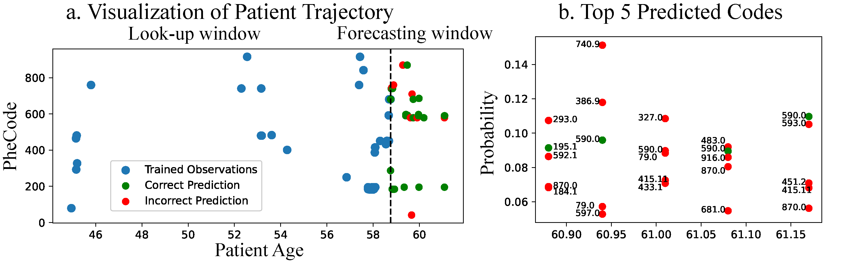
Figure 4. a. Visualization of patient medical trajectory from the PopHR dataset. Correct prediction is identified when the top 5 predicted PheCodes match the groundtruth. b. The top 5 predicted PheCodes for the final 5 timesteps of this trajectory.

4.4. An Example of Forecasting Trend Signal

We qualitatively analyzed ultra-long-term forecasting for TimelyGPT against leading baselines (PatchTST and DLinear) and ablating methods (GPT-2 and GPT-2 with RoPE), focusing on sleep stage transitions. We utilized 2,000-timestep look-up window and 6,000-timestep forecasting window. Forecasting beyond 2,000 timesteps is marked as extrapolation, as it exceeds the training length.

In the rectal temperature (i.e., trend signal), TimelyGPT forecasted results that align well with the groundtruth, effectively capturing distinct trend patterns (Fig. 3.b). Notably, the small bump in the prompt before the 1000-th timestep is a typical indicator for temperature drop. Most models are able to capture it except for DLinear, showing the benefits of pre-training. Beyond the training length of 4000, TimelyGPT demonstrated impressive extrapolation by accurately predicting the rise of the rectal temperature at around 7000-th timestep whereas PatchTST and GPT failed to achieve. As a result, the ability to model long-term trends crucially contributes to TimelyGPT’s extrapolation capabilities. We also visualized a EEG periodic biosignal and found similar conclusion (Fig. 9). In contrast, both PatchTST and vanilla GPT experience performance decline, suggesting a dependency on linear mapping as discussed in Section. 2.4 and in previous research (Li et al., 2023). TimelyGPT exhibits superior extrapolation capabilities over the ablating baseline GPT with RoPE, highlighting its effective trend pattern modeling for extrapolation.

4.5. Forecasting Clinical Diagnosis

Setup

We extracted irregularly-sampled time series from patient medical diagnosis histories in the PopHR database. We converted ICD-9 diagnosis codes to phenotype codes (PheCodes) using the expert-defined PheWAS catalog (Denny et al., 2013, 2010). we selected 315 unique PheCodes each with over 50,000 token counts and excluded patients who had fewer than 50 PheCode tokens. This resulted in a dataset of 489,000 patients, averaging 112 PheCodes each, divided into training (80%), validation (10%), and testing (10%) sets. We pre-trained on the entire training set and fine-tuned on a 20% subset of training data. We used cross entropy and top-$K$ recall to evaluate pre-training and fine-tuning, respectively. For forecasting, we set the look-up window to be be 50 timestamps and the rest as the forecasting window, which contain up to 100 timestamps (i.e., diagnosis codes).

For our TimelyGPT, we separately evaluated the performance of trajectory-based and time-specific inferences (Section 3.2). We compared with several transformer baselines including Informer, Fedformer, AutoFormer, and PatchTST as well as models designed for irregularly-sampled time series namely mTAND (Shukla and Marlin, 2021) and SeFT (Horn et al., 2020). Based on the scaling law in Section 4.2, we set model parameters for all transformers to about 6 million, with specific architectures and parameters detailed in Table 6.

Table 2. Forecasting results of TimelyGPT and 6 baselines on PopHR’s irregular-sampled time-series dataset.

Metrics	Recall @$K$ (%)
	$K=5$	$K=10$	$K=15$
TimelyGPT (trajectory-based)	52.30	64.35	77.12
TimelyGPT (time-specific)	58.65	70.83	82.69
Informer	46.37	60.14	71.24
Autoformer	42.87	57.43	68.59
Fedformer	43.31	58.34	69.60
PatchTST	48.17	65.55	73.31
MTand	52.59	70.21	83.73
SeFT	49.26	68.10	79.39

Results

TimelyGPT with time-specific inference outperformed the baselines with the top recall scores at $K={5,10,15}$, reaching 58.65%, 70.83%, and 82.69% respectively (Table 2). Moreover, the time-specific inference outperformed the trajectory-based inference, highlighting the advantage of time decay mechanism. Fig. 4.a displays the observed and predicted trajectory of a patient with neoplasm and genitourinary diseases. TimelyGPT produced a high top-5 recall rate of 85.7% on this patient. Indeed, most of the observed codes are among the top 5 predicted codes by the time-specific TimelyGPT. Zooming into the forecast window (Fig. 4.b), TimelyGPT accurately predicted Phecodes 590.0 (Pyelonephritis) three times around the age of 61. TimelyGPT predicted PheCode 740.9 at age 61 with high probability, which appears twice at ages 52 and 53 in the look-up window, reflecting model’s attention to historical contexts. Therefore, TimelyGPT demonstrates a promising direction to forecast patient health state despite the challenges inherent in modeling irregularly-sampled longitudinal EHR data.

4.6. Classification and Regression of Biosignals

Setup

For classification, we pre-trained on the Sleep-EDF (Kemp et al., 2000) and PTB-XL datasets (Alday et al., 2020) separately. Subsequently, the PTMs were fine-tuned on the Sleep-EDF, Epilepsy (Andrzejak et al., 2001), PTB-XL, and EMG (Goldberger et al., 2000) datasets. For regression, we pre-trained on both PTB-XL and PPGDalia datasets (Reiss et al., 2019a), followed by fine-tuning on the IEEEPPG (Zhang et al., 2015), RR, HR, and SpO2 (Tan et al., 2021) datasets. Each dataset was split into a training (80%), validation (10%), and test (10%) sets. When both pre-training and fine-tuning on the same dataset, we fine-tuned the PTMs using 20% of the training set. We used accuracy and MAE as evaluation metrics for classification and regression, respectively.

We assessed various transformer baselines, including PatchTST (Nie et al., 2023), AutoFormer (Wu et al., 2022), FedFormer (Zhou et al., 2022), TimesNet (Wu et al., 2023), TST (Zerveas et al., 2020), and CRT (Zhang et al., 2023) as well as consistency-based PTMs including TS-TCC (Eldele et al., 2021), TS2Vec (Yue et al., 2022), and TF-C (Zhang et al., 2022b). Based on the scaling law in Section 4.2, we assigned model parameters of 18M for Sleep-EDF and 7.5M for PTB-XL datasets. Details about specific architectures and parameters are provided in Table 6.

Results

As shown in Table 8, TimelyGPT achieved the best performance in classifying Epilepsy and EMG and in the regression of IEEEPPG, HR, and SpO2. This superiority highlights the potential of the generative pre-training framework to generalize across datasets (Radford et al., 2019). On the other hand, CRT stood out the best when both pre-training and fine-tuning were conducted on the same dataset. Our TimelyGPT outperformed PatchTST for dealing with long sequences, especially in the Sleep-EDF and PTB-XL datasets. This suggests that our proposed convolution-subsampling tokenizer might be more effective at extracting dense information from long sequences. Masking-based transformer PTMs performed poorly due to the distribution shift issue (Zhang et al., 2023). Models like Autoformer, Fedformer, and TimesNet, which rely on time decomposition and frequency-domain information, were especially affected bydistribution shift. Furthermore, consistency-based PTMs and recurrent models generally exhibited lower performance in these tasks.

4.7. Classification of Irregular Time-Series

Setup

PopHR provides rule-based labels for 12 phenotypes, facilitating multi-label classification. For each disease label, we calculated the prevalence ratio of each PheCode across the true patients and the patient population, selecting the PheCodes with a ratio above 5. We excluded patients with fewer than 10 PheCodes, yielding a dataset comprising 47,000 patients and 8.4 million records. We used cross entropy and Area under Precision Recall Curve (AUPRC) to evaluate pre-training and fine-tuning, respectively.

We compared TimelyGPT with the PTMs, which have demonstrated efficiency in Section 4.6, including PatchTST, TST, CRT, TS-TCC, and TF-C. We also assessed algorithms designed for irregularly-sampled time series, including mTAND (Shukla and Marlin, 2021), GRU-D (Che et al., 2018), SeFT (Horn et al., 2020), and RAINDROP (Zhang et al., 2022a). Based on the scaling law in Section 4.2, we set model parameters for all transformers to around 3 million, with specific architectures and parameters detailed in Table 6.

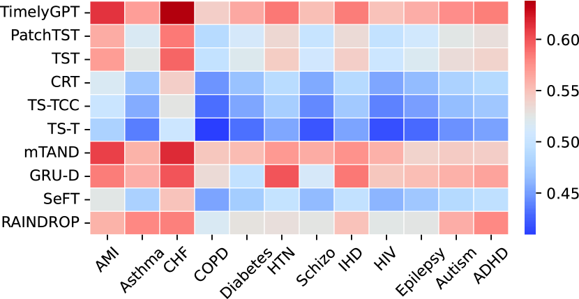
Figure 5. The heatmap displays AUPRC of 9 baselines (rows) and 12 phenotypes (columns) on the PopHR’s irregular-sampled time-series. Full results is available in Table 9.

Results

In Fig. 5, TimelyGPT outperformed other PTMs by adeptly modeling trend patterns and handling unequal time intervals. This highlights the shortcomings of absolute position embedding, which struggles with phase shifting issue in irregular sequences (Sinha et al., 2022). With the aid of time decay, TimelyGPT surpassed other methods designed for irregularly-sampled time series, leading with an average AUPRC of 57.6% and outperforming the next best mTAND (56.4%).

4.8. Ablation Study

To assess the contributions of various components in TimelyGPT, we conducted ablation studies by selectively omitting components including convolution subsampling tokenizer, temporal convolution module, exponential decay, and RoPE relative position embedding. Notably, removing all components results in a vanilla GPT-2. Since exponential decay in xPos depends on RoPE, we cannot assess the impact of exponential decay independently by removing the RoPE component. Since we already ablated the forecasting experiment in Section 4.4, we focused this ablation study on the classification experiments on the Sleep-EDF and PopHR datasets (CHF phenotype only), corresponding to continuous and irregularly-sampled time series, respectively. The models were pre-trained and then fine-tuned on the same dataset.

Table 3. Ablation results of TimelyGPT w/o specific components in terms of downstream classification accuracy.

Method / Classification	Sleep-EDF	PopHR(CHF)
TimelyGPT (with Pre-training)	89.21	64.89
w/o Convolution Subsampling	88.65	—
w/o Temporal Convolution	87.65	63.21
w/o Exponential Decay	86.52	55.36
w/o RoPE (GPT-2)	84.25	51.83
TimelyGPT (w/o Pre-training)	85.32	64.06

In Table 3, for the Sleep-EDF classification, RoPE was the main contributor to the improvement over the baseline GPT-2, followed by exponential decay. Relative position embedding in TimelyGPT was found to effectively model temporal dependencies. Moreover, by integrating convolution modules, TimelyGPT was able to capture local features, achieving close performance to other transformers. However, the convolution modules had limited benefits for irregular-sampled time-series, possibly due to its discrete nature. By mitigating the effects of distant diagnoses, exponential decay encodes trend patterns into the modeling of patients’ health trajectory, making it promising for irregular time-series analysis. Pre-training conferred a notable increase of 3.89% in the classification of continuous biosignals, while the improvement was less evident in irregularly-sampled time series (0.83%).

5. Conclusion and Future Work

TimelyGPT effectively forecasts long sequence of time-series, utilizing xPos embedding, recurrent attention, and convolution modules. It can accurately extrapolates up to 6,000 timesteps given only a 2000-timestep prompt. Moreover, TimelyGPT also effectively forecasts irregularly-sampled time series by conditioning the recurrent Retention on the time. TimelyGPT’s superiority in classification and regression tasks for both continuous and irregularly-sampled time series is also attributable to its temporal convolution module and time decay mechanism. In our future work, we will perform comprehensive and in-depth analysis on the trajectory inference of the EHR data as it may have a profound impact on future of patient care and early intervention. TimelyGPT is a causal model with unidirectional attention (Press et al., 2022). This may limits its expressiveness in terms of time-series representation learning, which may be improved via a bidirectional architecture. To enhance transfer learning, we would adapt TimelyGPT for out-of-distribution biosignals, further enhancing its utility in healthcare time-series.

Appendix A Revisiting Time-Series Transformers

A.1. Review of Existing Works

Efficient Attention in Transformer: Transformer models have found extensive applications in both the Natural Language Processing and Computer Vision domains (Vaswani et al., 2023). In the vanilla self-attention mechanism, the query, key, value matrices are denoted as ${\bm{Q}},{\bm{K}},{\bm{V}}\in\mathbb{R}^{N\times d}$. The output embedding for the $n$-th token is represented as ${\bm{O}}_{n}=\frac{\sum_{m}^{N}\text{sim}({\bm{Q}}_{n},{\bm{K}}_{m}){\bm{V}}_{m}}{\sum_{m}^{N}\text{sim}({\bm{Q}}_{n},{\bm{K}}_{m})}$, where the the similarity function represents the softmax of inner-product $\text{sim}({\bm{Q}}_{n},{\bm{K}}_{m})=\exp({\bm{Q}}_{n}{\bm{K}}_{m}^{\top}/\sqrt{d})$. The self-attention mechanism, also known as token-mixer, aims to integrate information from every token and thus capture global-range interaction. However, computing the dot product ${\bm{Q}}_{n}{\bm{K}}_{m}^{\top}$ before the softmax operation introduces computational complexity of $O(N^{2}d)$. As sequence length increases, this quadratic complexity becomes bottleneck, making it challenging to train for longer sequences. Numerous studies have been proposed to address the quadratic issue in self-attention mechanism. The linear attention replaces the softmax term $\text{sim}({\bm{Q}}_{m},{\bm{K}}_{m})$ with $\phi({\bm{Q}}_{n})\phi({\bm{K}}_{m}^{\top})$ for a nonlinear kernel function $\phi(\cdot)$ (Katharopoulos et al., 2020), avoiding the quadratic computation.

Recent research has explored alternatives to the token-mixer attention mechanism including Multi-Layer Perceptron (MLP) (Tolstikhin et al., 2021), convolution (Poli et al., 2023), and RNN (Peng et al., 2023; Sun et al., 2023). Particularly, RNN-variant models like RWKV and RetNet have successfully scaled up to more than 14 billion parameters, yielding comparable performance to conventional transformers. A fascinating connection between linear attention and RNNs has been identified (Katharopoulos et al., 2020), making RNN-based token mixer as efficient as linear attention. The output embedding from linear attention can be recast as an RNN: ${\bm{O}}_{n}=\frac{\phi({\bm{Q}}_{n})\sum_{m}^{N}\phi({\bm{K}}_{m}^{\top}){\bm{V}}_{m}}{\phi({\bm{Q}}_{n})\sum_{m}^{N}\phi({\bm{K}}_{m}^{\top})}=\frac{\phi({\bm{Q}}_{n}){\bm{S}}_{n}}{\phi({\bm{Q}}_{n}){\bm{Z}}_{n}}$, where ${\bm{S}}_{n}=\sum_{m}^{N}\phi({\bm{K}}_{m}^{\top}){\bm{V}}_{m},\,{\bm{Z}}_{n}=\sum_{m}^{N}\phi({\bm{K}}_{m}^{\top})$. Thus, the output embedding ${\bm{O}}_{n}$ depends on both ${\bm{S}}_{n}$ and ${\bm{Z}}_{n}$, which are incrementally updated through cumulative sums. Thus, the RNN-based token-mixer not only competes in performance, but also offers linear training and consistent inference complexities. By employing exponential decay mechanism, it diminishes the influence of distant positions, transitioning from “token-mixing” to “time-mixing”. Considering RNN’s historical effectiveness in time-series and audio domains, it stands out as an excellent choice for temporal modeling.

State Space Model: Recent advancements in deep state-space models (SSMs) have led to significant improvements in long sequence modeling across areas including Natural Language Processing, Computer Vision, audio, and time-series (Gu et al., 2022). These models learn continuous or discrete-time representation, transforming input signals into output via state variables. Mainstream sequence models face memory forgetting issues, such as the fixed-size context windows of Transformer and the vanishing gradient in RNNs. In response, HiPPO presents a closed-form solution adept at preserving historical information efficiently. Its variant HiPPO-LegS not only addresses vanishing gradients but also provides timescale robustness, ensuring resilience to different sampling intervals. Furthermore, the Hungry Hungry Hippos (H3) model exhibits capabilities to recall early tokens and draw information throughout a sequence. However, SSMs often fail to leverage content-aware variables as Transformer. In this context, the RetNet model can be likened to the Structured State Space Sequence (S4) model (Gu et al., 2022), especially when queries and keys are not dependent on data.

Time-series Transformer: Transformers are increasingly applied in LTSF tasks, attributed to their capabilities in capturing long-term temporal dependencies (Zhou et al., 2021; Wu et al., 2022; Zhou et al., 2022; Woo et al., 2022; Nie et al., 2023). Researchers have modified transformers by incorporating custom attention modules to address complex temporal dependencies (Zhou et al., 2021; Wu et al., 2022; Zhou et al., 2022). Studies like (Wu et al., 2022; Zhou et al., 2022; Woo et al., 2022) have introduced time-decomposition techniques into attention mechanisms to bolster modeling capability. The majority of studies focus on the encoder-decoder architecture, coupled with a one-forward prediction framework (Zhou et al., 2021). In this design, the decoder takes a concatenated input of the context (or prompt) and placeholder forecasting windows, directly generating the resulting embedding without autoregressive decoding. As a result, these models aim to avoid error accumulation seen in autoregressive frameworks, but aligning its performance closely with linear models (Zeng et al., 2022). Encoder-only models, like patchTST, use the encoded embedding for forecasting with the help of a linear layer (Nie et al., 2023). Additionally, self-supervised representation learning techniques in time series, such as TS2Vec and TimesNet, offer valuable representation learning capabilities for forecasting tasks (Yue et al., 2022; Wu et al., 2023).

Challenges for Time-series Transformer Models: Recent studies show that transformers are limited in time-series forecasting (Zeng et al., 2022). The permutation-invariant nature of self-attention and the limitations of position embedding have been cited as potential issues, leading some to argue that transformers may not significantly outperform traditional models in this domain.

A.2. Forecasting Transformer Models

In the forecasting experiment, we conducted a comparison between our proposed TimelyGPT and other models such as encoder-decoder transformers (such as Informer, Autoformer, and Fedformer) and encoder-only transformer (PatchTST). The encoder-decoder architecture utilizes one-forward decoding instead of autoregressive decoding, which is hard to generate effective representation of future timesteps. The PatchTST model exclusively focuses on encoding embedding of input sequence. Both encoder-decoder and encoder-only architectures lack the ability to generate representative embedding of future time and instead rely on linear layers for forecasting. It is important to note that both encoder-decoder and encoder-only transformers lack the ability to extrapolate due to the presence of absolute position embedding.

Table 4. Properties of transformer for time-series forecasting.

Method	Arch	Rely Linear Layer	Extrapolation
TimelyGPT	Decoder	No	Yes
Informer	Enc-Dec	Yes	No
Autoformer	Enc-Dec	Yes	No
Fedformer	Enc-Dec	Yes	No
PatchTST	Encoder	Yes	No

A.3. Pre-trained Models for Classification and Regression

For the time-series classification and regression tasks, we compared our proposed TimelyGPT with forecasting transformers (such as Autoformer, Fedformer, and PatchTST), transformer-based PTMs (TST and CRT), and consistency-based PTMs (TS-TCC and TF-C). Forecast transformers utilize the pre-training strategy with the mask introduced by (Zerveas et al., 2020). Additionally, both TST and CRT utilize pre-training strategies that involve masking and droping task. The consistency-based PTMs, TS-TCC and TF-C, propose contextual contrasting modules that utilize the contexts from the temporal contrasting module.

Appendix B Details about TimelyGPT

B.1. From Absolute to Relative Position Embedding

Unlike RNNs or CNNs, the inclusion of positional embedding is essential for the Transformer model. Since the permutation-invariant self-attention mechanism cannot capture input order, making it challenging to differentiate tokens in various positions. The solution fall into two categories: (1) incorporate position information into the inputs, i.e., absolute position embedding; (2) modify the attention matrix to distinguish tokens at different positions, referring to relative position embedding.

In absolute position embedding, the token representation for a given token $n$ consists of a word embedding ${\bm{X}}_{n}$ and a position embedding ${\bm{P}}_{n}$. The self-attention mechanism is expressed as:

$${\bm{Q}}_{n}=({\bm{X}}_{n}+{\bm{P}}_{n}){\bm{W}}_{Q},\quad{\bm{K}}_{n}=({\bm{X}}_{n}+{\bm{P}}_{n}){\bm{W}}_{K},\quad{\bm{V}}_{n}=({\bm{X}}_{n}+{\bm{P}}_{n}){\bm{W}}_{V}$$

(6) $${\bm{A}}_{n,m}=\text{softmax}({\bm{Q}}_{n}{\bm{K}}_{m}^{\top}),\quad{\bm{O}}_{m}=\sum_{m}{\bm{A}}_{n,m}{\bm{V}}_{m}$$

where ${\bm{A}}_{n,m}$ is an attention score between token $n$ and $m$ without scaling. The inner-dot product ${\bm{Q}}_{n}{\bm{K}}_{m}^{\top}$ and output embedding ${\bm{O}}_{m}$ can be expanded as follows:

$${\bm{Q}}_{n}{\bm{K}}_{m}^{\top}=({\bm{X}}_{n}+{\bm{P}}_{n}){\bm{W}}_{Q}(({\bm{X}}_{m}+{\bm{P}}_{m}){\bm{W}}_{K})^{\top}$$

$$=({\bm{X}}_{n}+{\bm{P}}_{n}){\bm{W}}_{Q}{\bm{W}}_{K}^{\top}({\bm{X}}_{m}+{\bm{P}}_{m})^{\top}$$

(7) $$=\underbrace{{\bm{X}}_{n}{\bm{W}}_{Q}{\bm{W}}_{K}^{\top}{\bm{X}}_{m}^{\top}}_{\text{token-token}}+\underbrace{{\bm{X}}_{n}{\bm{W}}_{Q}{\bm{W}}_{K}^{\top}{\bm{P}}_{m}^{\top}}_{\text{token-position}}+\underbrace{{\bm{P}}_{n}{\bm{W}}_{Q}{\bm{W}}_{K}^{\top}{\bm{X}}_{m}^{\top}}_{\text{position-token}}+\underbrace{{\bm{P}}_{n}{\bm{W}}_{Q}{\bm{W}}_{K}^{\top}{\bm{P}}_{m}^{\top}}_{\text{position-position}}$$

(8) $${\bm{O}}_{n}=\sum_{m}\text{softmax}\left(({\bm{X}}_{n}{\bm{W}}_{Q}+{\bm{P}}_{n}{\bm{W}}_{Q})({\bm{W}}_{K}^{\top}{\bm{X}}_{m}^{\top}+{\bm{W}}_{K}^{\top}{\bm{P}}_{m}^{\top})\right)({\bm{X}}_{n}+{\bm{P}}_{m}){\bm{W}}_{V}$$

where attention arises from four types of interactions: (1) token-token interaction; (2) token-position interaction; (3) position-token interaction; (4) position-position interaction. However, absolute position embedding only incorporates fixed position information, neglecting the relative positional difference between the token $n$ and $m$.

In the realm of audio processing, prevalent transformers like Conformer (Gulati et al., 2020) incorporate relative positional information through the T5 position embedding (Raffel et al., 2020). Notably, the T5 model suggests a minimal interaction between tokens and positions, resulting in the exclusion of token-position and position-token terms from the attention matrix:

(9) $${\bm{Q}}_{n}{\bm{K}}_{m}^{\top} ={\bm{X}}_{n}{\bm{W}}_{Q}{\bm{W}}_{K}^{\top}{\bm{X}}_{m}^{\top}+{\color[rgb]{1,0,0}\beta_{n,m}}$$

where the position-position interaction term, ${\bm{P}}_{n}{\bm{W}}_{Q}{\bm{W}}_{K}^{\top}{\bm{P}}_{m}^{\top}$, is replaced with a trainable bias related to the position $n$ and $m$. The T5 position embedding follows Transformer-XL, omitting the position term ${\bm{P}}_{m}{\bm{W}}_{V}$ in the attentive aggregation computation (Dai et al., 2019; Yang et al., 2020). As a result, the relative position embedding is only added to the dot product ${\bm{Q}}{\bm{K}}^{\top}$:

(10) $${\bm{O}}_{n}=\sum_{m}\text{softmax}({\bm{X}}_{n}{\bm{W}}_{Q}{\bm{W}}_{K}^{\top}{\bm{X}}_{m}^{\top}+{\color[rgb]{1,0,0}\beta_{n,m}}){\bm{X}}_{m}{\bm{W}}_{V}$$

The RoPE technique leverages the property of rotation matrix to model positional information (Su et al., 2022). To incorporate this relative position information into the queries ${\bm{Q}}$ and keys ${\bm{K}}$, the method aims to identify functions $f_{{\bm{Q}}}({\bm{Q}},\cdot)$ and $f_{K}({\bm{K}},\cdot)$ that satisfies this invariant criteria about relative distance:

(11) $$\left\langle{\bm{Q}}_{n},{\bm{K}}_{m}\right\rangle=\left\langle f_{{\bm{Q}}}({\bm{Q}},n),f_{K}({\bm{K}},m)\right\rangle=g({\bm{Q}},{\bm{K}},m-n),$$

where $g$ is a function that depends only on the relative distance $m-n$ and ${\bm{Q}}={\bm{X}}{\bm{W}}_{Q}$ and ${\bm{K}}={\bm{X}}{\bm{W}}_{K}$ stand for token embedding for queries and keys matrices, respectively. RoPE defines the function $f$ involving a $d$-dimensional rotation matrix ${\bm{R}}$:

(12) $$f_{{\bm{Q}}}({\bm{Q}},n)={\bm{R}}^{d}_{\Theta,n}({\bm{X}}_{n}{\bm{W}}_{Q}),\quad f_{{\bm{K}}}({\bm{K}},m)={\bm{R}}^{d}_{\Theta,m}({\bm{X}}_{m}{\bm{W}}_{K})$$

With a given hidden size $d$, a block diagonal matrix ${\bm{R}}^{d}_{\Theta,n}$ contains multiple rotation matrices $({\bm{R}}^{(1)}_{n,\theta_{1}},\dots,{\bm{R}}^{(d/2)}_{n,\theta_{d/2}})$ on its diagonal:

(13) $${\bm{R}}^{d}_{\Theta,n}=\begin{bmatrix}{\bm{R}}^{(1)}_{n,\theta_{1}}&&\\ &\ddots&\\ &&{\bm{R}}^{(d/2)}_{n,\theta_{d/2}}\end{bmatrix},\quad{\bm{R}}^{(i)}_{n,\theta_{i}}=\begin{bmatrix}\text{cos}\ n\theta_{i}&-\text{sin}\ n\theta_{i}\\ \text{sin}\ n\theta_{i}&\text{cos}\ n\theta_{i}\end{bmatrix}$$

where the rotation hyperparameter $\theta_{i}=10000^{-2(i-1)/d}$. In RoPE, any even-dimension representation can be built by placing multiple 2-dimensional rotation matrices diagonally within the ${\bm{R}}^{d}_{\Theta,n}$ matrix, expanding hidden size from 2-dimension to $d$-dimension. As ${\bm{R}}^{d}_{\Theta,m-n}=({\bm{R}}^{d}_{\Theta,n})^{\top}{\bm{R}}^{d}_{\Theta,m}$, RoPE satisfies the property outlined in Eq 11:

$$\left\langle{\bm{Q}}_{n},{\bm{K}}_{m}\right\rangle=\sum_{i=1}^{d/2}\left\langle{\bm{Q}}_{n}[2i-1:2i],{\bm{K}}_{m}[2i-1:2i]\right\rangle$$

(14) $$=\sum_{i=1}^{d/2}{\bm{R}}^{d}_{\theta_{i},m-n}\left\langle({\bm{X}}_{n}{\bm{W}}_{Q})[2i-1:2i],({\bm{X}}_{m}{\bm{W}}_{K})[2i-1:2i]\right\rangle$$

In RoPE, relative position information is added to the inner product ${\bm{Q}}{\bm{K}}^{\top}$ by rotating the angles of queries and keys matrices. Recently, (Sun et al., 2022) argues that the sinusoids used in the rotation matrices do not change monotonically. Instead, they oscillate dramatically as the relative distance increases. This limitation hinders RoPE’s ability to sequences of extended lengths. To address it, (Sun et al., 2022) proposes xPos that preserves the advantage of ROPE and behaves stably at long-term dependency by measuring position monotonicity (Sun et al., 2022).

B.2. Equivalence of Three Forward-pass Retention

According to Section 3.2, the parallel forward-pass is equivalent to the recurrent forward-pass. With the initial state variable ${\bm{S}}_{0}=0$, the recurrent forward-pass can be expressed as follows:

$$\textbf{Recurrent: }{\bm{S}}_{n}=\underbrace{{\bm{K}}_{n}^{\top}{\bm{V}}_{n}}_{\text{Single-token}}+\gamma{\bm{S}}_{n-1},\quad\text{Ret}({\bm{X}}_{n})={\bm{Q}}_{n}{\bm{S}}_{n}$$

(15) $$\implies{\bm{S}}_{n}=\sum_{m}^{n}\gamma^{n-m}{\bm{K}}_{m}^{\top}{\bm{V}}_{m},\quad\text{Ret}({\bm{X}}_{n})={\bm{Q}}_{n}\sum_{m}^{n}\gamma^{n-m}{\bm{K}}_{m}^{\top}{\bm{V}}_{m}$$

where $\text{Ret}({\bm{X}}_{n})$ calculates the Retention at single-time $n$ by considering timestep $i$ up to the current time. It corresponds to the $n$-th timestep (row) of parallel forward-pass of Retention.

$$\textbf{Recurrent: }\text{Ret}({\bm{X}}_{n})={\bm{Q}}_{n}\sum_{m}^{n}\gamma^{n-m}{\bm{K}}_{m}^{\top}{\bm{V}}_{m}$$

(16) $$\implies\textbf{Parallel: }\text{Ret}({\bm{X}}_{n})=\underbrace{{\bm{Q}}_{n}}_{1\times d_{qk}}\underbrace{{\bm{K}}_{m\leq n}^{\top}}_{d_{qk}\times n}\underbrace{\odot{\bm{D}}_{m\leq n}}_{n\times n}\underbrace{{\bm{V}}_{m\leq n}}_{n\times d_{v}}$$

When the recurrent forward-pass traverses all timesteps, the parallel and recurrent forward-passes of Retention become identical. With the parallel and recurrent forward-passes of Retention, we aim to show the equivalence between tje chunk-wise forward-pass and the parallel and recurrent forward-passes. The computation of chunk-wise Retention involves both parallel intra-chunk and recurrent inter-chunk computation as follows.

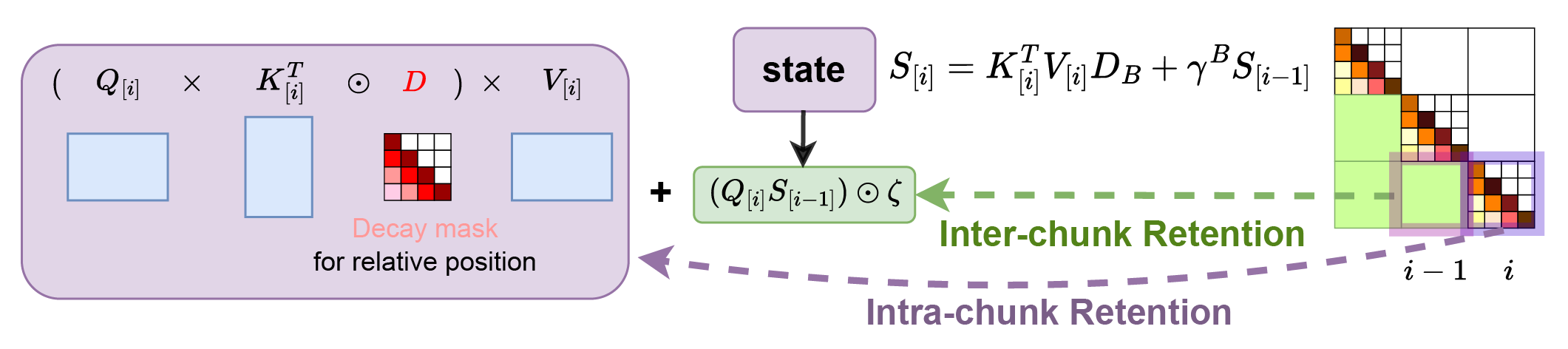
Figure 7. Chunk-wise forward-pass of Retention. It can be represented as parallel inner-chunk information (highlighted as purple) as well as recurrent inter-chunk information (highlighted as green) with the help of state variable ${\bm{S}}$.

$$\textbf{Chunk-wise: }\text{Ret}({\bm{X}}_{[i]})=\underbrace{({\bm{Q}}_{[i]}{\bm{K}}_{[i]}^{\top}\odot{\bm{D}}){\bm{V}}_{[i]}}_{\text{Intra-chunk}}+\underbrace{({\bm{Q}}_{[i]}{\bm{S}}_{[i-1]})\odot\zeta}_{\text{Inter-chunk}}$$

(17) $${\bm{S}}_{[i]}=\underbrace{{\bm{K}}_{[i]}^{\top}({\bm{V}}_{[i]}\odot{\bm{D}}_{B})}_{\text{Current chunk}}+\underbrace{\gamma^{B}{\bm{S}}_{[i-1]}}_{\text{Past chunk}},\,\zeta_{j}=\gamma^{j}$$

where $\zeta=[\gamma^{1},\gamma^{2},\ldots,\gamma^{B}]^{\top}$ is a column-vector of time-decay scaling factor for inter-chunk attention between the current chunk $[i]$ and the previous chunk $[i-1]$. Specifically, $\gamma^{j}$ is the scaling factor for the $j^{th}$ row of chunk $[i]$ from the last row of chunk $[i-1]$ such that the bigger the $j$ index the smaller the $\gamma^{j}$ value. Therefore, Retention recursively aggregates information from the $i$-th chunk (i.e., intra-chunk embedding) and the previous chunk (i.e., inter-chunk embedding).

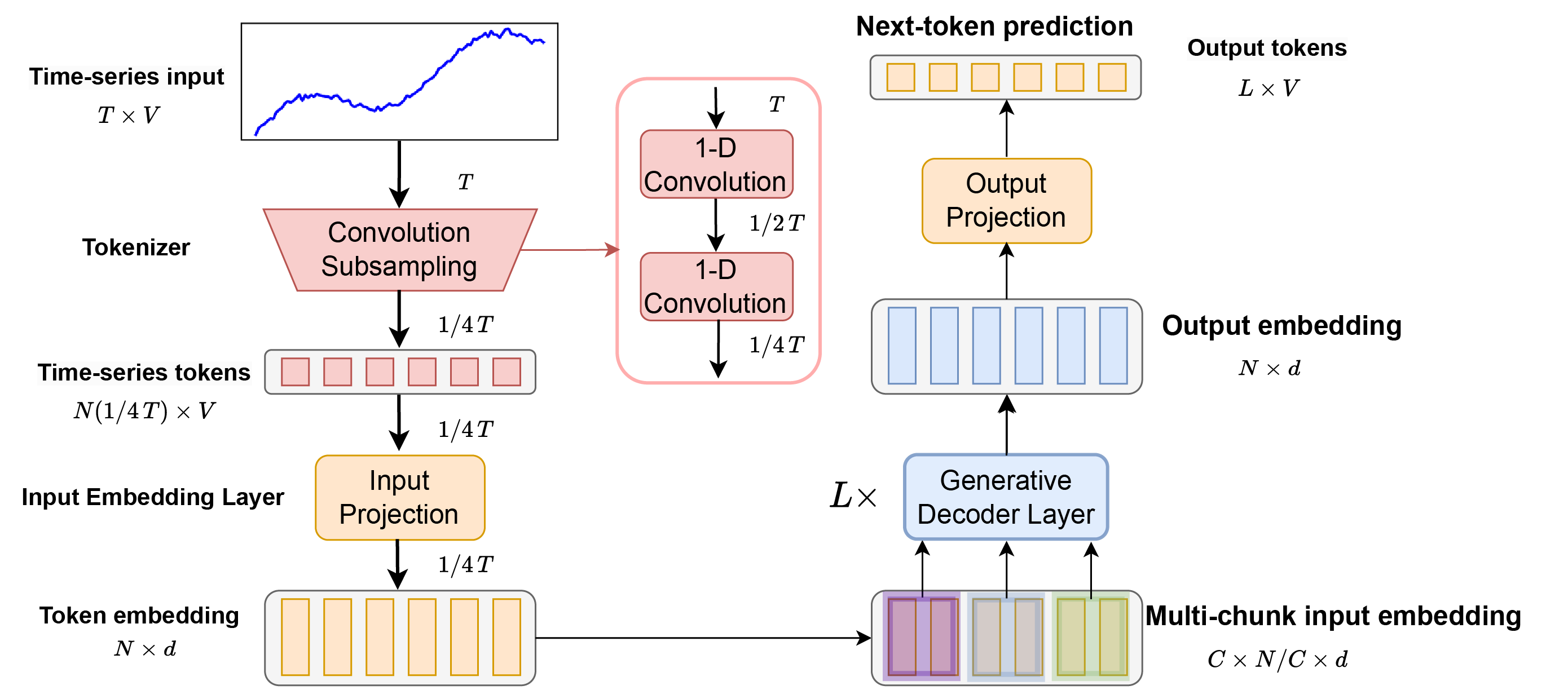
Figure 8. Schematic of the TimelyGPT Pre-Training Process

For the per-chunk state variable ${\bm{S}}_{[i]}$, it computes current-chunk information as well as past-chunk information. The current-chunk information ${\bm{K}}_{[i]}^{\top}{\bm{V}}_{[i]}$ decays by ${\bm{D}}_{B}$, which is the last row of decay matrix ${\bm{D}}$. The past chunk information ${\bm{S}}_{[i-1]}$ is decayed with respect to the chunk size $B$. The initial state variable ${\bm{S}}_{[i=0]}=0$ is computed recurrently given the chunk size $B$:

(18) $${\bm{S}}_{[i]}={\bm{K}}_{[i]}^{\top}({\bm{V}}_{[i]}\odot{\bm{D}}_{B})+\gamma^{B}{\bm{S}}_{[i-1]}=\sum_{m=1}^{B}\gamma^{B-m}{\bm{K}}_{m}^{\top}{\bm{V}}_{m}+\gamma^{B}{\bm{S}}_{[i-1]}$$

Moreover, the update of state variable ${\bm{S}}_{[i]}$ can be reformulated in parallel. The first term represents the information of current chunk, and the second term represented the past-chunk information decayed by the chunk size ${\bm{B}}$. Consequently, ${\bm{S}}_{[i-1]}$ represents the state information from the beginning to the $(i-1)$-th chunk, and we represent the inter-chunk information in chunk-wise Retention:

$${\bm{S}}_{[i-1]}=\sum_{m=1}^{B*i}\gamma^{B*i-m}{\bm{K}}_{m}^{\top}{\bm{V}}_{m}={\bm{K}}^{\top}_{1:(B*i)}\odot{\bm{D}}_{1:(B*i)}{\bm{V}}_{1:(B*i)}$$

$$\underbrace{({\bm{Q}}_{[i]}{\bm{S}}_{[i-1]})\odot\zeta}_{\text{Inter-chunk}}=({\bm{Q}}_{(B*i):(B*(i+1))}{\bm{K}}^{\top}_{1:(B*i)}\odot{\bm{D}}_{1:(B*i)}{\bm{V}}_{1:(B*i)})\odot\zeta$$

(19) $$={\bm{Q}}_{(B*i):(B*(i+1))}{\bm{K}}^{\top}_{1:B*i}\odot{\bm{D}}_{(B*i):(B*(i+1))}{\bm{V}}_{1:(B*i)}$$

where the intra-chunk computation updates each row of the lower triangular matrix (highlighted as green in Fig. 7). Together, the recurrent intra-chunk computation with the parallel intra-chunk computation (highlighted as purple 7) completes the chunk-wise forward-pass of Retention.

B.3. TimelyGPT Pre-training Overflow

For the TimelyGPT pre-training, we illustrate the full processes of input processing, model training, and next-token prediction in Fig. 8. For a time-series input with $T$ timesteps and $V$ variates, it is tokenized via a convolution-subsampling module. This tokenizer, typically comprising two 1-D convolution layers with a kernel size of 3 and stride of 2. It produces a sequence of tokens of the shape $N\times V$, effectively reducing the sequence length to 1/4, i.e., $N=1/4T$. The sequence of tokens is projected into an input embedding of the shape $L\times d$ with an linear projection layer. As a result, the input embedding is passed through $L$ generative decoder layers, where the Retention mechanism takes segmented mulitple-chunk input embedding. Finally, the output embedding of the shape $N\times d$ is passed through an output projection layer, which generate a sequence of tokens with the shape of $L\times V$ for next-token prediction.

Table 5. Description of datasets utilized for forecasting, classification, and regression tasks.

Details	Task	Variates	Timesteps	Sequences	length	Classes
Sleep-EDF (Kemp et al., 2000)	Forecasting	7	1.2B	300.5K	4,000	None
Sleep-EDF (sleep) (Kemp et al., 2000)	Classification	1	586.4M	195.5K	3,000	5
Epilepsy (Andrzejak et al., 2001)	Classification	1	2.0M	11.5K	178	2
PTB-XL (Alday et al., 2020)	Classification	12	109.2M	21,837	5,000	5
EMG (Goldberger et al., 2000)	Classification	1	306.0K	204	1,500	3
PPG-Dalia (Reiss et al., 2019a)	Regression	4	16.6M	64,697	256 & 512∗	None
IEEEPPG (Zhang et al., 2015)	Regression	5	3.1M	3,096	1,000	None
RR (Pimentel et al., 2017)	Regression	2	31.5M	7,870	4,000	None
HR (Pimentel et al., 2017)	Regression	2	31.8M	7,949	4,000	None
SpO2 (Pimentel et al., 2017)	Regression	2	31.8M	7,949	4,000	None

^∗ The sequence length of the PPG-Dalia dataset varies across different dimensions.

Appendix C Additional Information for Experiments

C.1. Dataset Description

Sleep-EDF dataset for Forecasting. Sleep-EDF dataset proposed by (Kemp et al., 2000) from PhysioBank (Goldberger et al., 2000) contains sleep cassette data obtained from 153 subjects. The collected whole-night polysmnographic (PSG) sleep recordings encompass 7 features: Electroencephalogram (EEG) (from Fpz-Cz and Pz-Oz electrode locations), electrooculogram (EOG) (horizontal), submental chin electromyogram (EMG), and an event marker. EEG and EOG signals were sampled at 100 Hz, while the EMG and event marker were sampled at 1 Hz. The sleep patterns correspond to the PSGs consist of five sleep stages: Wake (W), Non-rapid eye movement (N1, N2, N3) and Rapid Eye Movement (REM). This dataset for ultra-long-term forecasting contains a total of 1.2B timesteps, segmented into 300.7K sequences of 4,000 timesteps each.

Sleep-EDF (Sleep-stage only) dataset for Classification. We leveraged only the sleep stage of the Sleep-EDF dataset for the classification task following existing studies (Eldele et al., 2021; Zhang et al., 2022b). In line with conventional practices, we selected the single EEG channel that captures signals from the Fpz-Cz electrode location. Since the Sleep-EDF dataset labels five sleep stages (i.e., W, REM, N1, N2 and N3), we only focused on EEG signals associated with these sleep stages, resulting in a total of 586.4 million timesteps. This dataset was segmented into 195.5K sequences, each with 3,000 timesteps.

Epilepsy Seizure Classification. Epileptic Seizure Recognition dataset (Andrzejak et al., 2001) comprises EEG measurements from 500 subjects. This dataset captures brain electrical activity from different regions and states, and are divided into segments of 23.6 seconds. The original dataset consists of five classes of EEG measuring eyes open, eyes closed, healthy brain region, tumor region, and seizure. The first four classes were merged into a single class as these classes are unrelated to epileptic seizure, enabling a binary classification of epileptic seizures. The dataset for classification consists of 2M timesteps, divided into 11.5K sequences, each containing 178 timesteps.

PTB-XL Classification. Physikalisch Technische Bundesanstalt large scale cardiology database (PTB-XL) (Alday et al., 2020) from PhysioBank (Goldberger et al., 2000) contains 21,837 clinical 12-lead ECG signals (male: 11,379 and female: 10,458) with a duration of 10 seconds each, sampled with a rate of 500 Hz. These signals are categorized based on a set of twelve leads (I, II, III, AVL, AVR, AVF, V1, V2, V3, V4, V5, V6), where the reference electrodes on the right arm are provided for each signal, resulting in twelve labels for classification. This dataset for classification comprises 21,837 samples, each spanning 5,000 timesteps, amounting to a total of 109.2M timesteps.

EMG Classification. EMG dataset from PhysioBank (Goldberger et al., 2000) captures the electrical activity resulting from neural stimulation of muscles. This dataset provides insights about muscle functionality and the corresponding nerves responsible for their control. This dataset contains single-channel EMG signals sampled with a rate of 4 KHz. EMG recordings were obtained from the tibialis anterior muscle of volunteers exhibiting different degrees of muscular and neural disorders, resulting in three classification labels. This dataset for classification comprises 306.0K timesteps, segmented into 204 sequences, each consisting of 1,500 timesteps.

PPG-Dalia Regression. PPG-Dalia dataset (Reiss et al., 2019a) is available from Monash University, UEA&UCR Time Series Regression Archive (Tan et al., 2021). This dataset captures photoplethysmograph (PPG) data for motion compensation and heart rate estimation. Data was collected from 15 subjects engaging in daily life activities using both wrist-worn (Empatica E4) and chest-worn (RespiBAN Professional) devices. All signals were sampled at 700 Hz. The ECG recording serve as a ground truth for heart rate. The PPG and 3D-accelerometer data are used to estimate heart rate, while accounting for motion artefacts. This dataset with a total of 16.6M timesteps was divided into 64,697 sequences, with varied lengths of 256 or 512 timesteps in different dimensions. The pre-training on this PPG-Dalia as well as the PTB-XL dataset was utilized for fine-tuning regression tasks.

IEEEPPG Regression. IEEEPPG dataset (Zhang et al., 2015) is sourced from Monash University, UEA&UCR Time Series Regression Archive (Tan et al., 2021). This dataset aims to estimate heart rate by utilizing PPG and ECG signals. The dataset includes two-channel PPG signals, three-axis acceleration signals, and one-channel ECG signals. These signals were recorded simultaneously and sampled at a rate of 125 Hz. This dataset for regression contains 3.1M timesteps, segmented into 3.096K sequences of 1,000 timesteps each.

RR, HR and SpO2 Regression. BIDMC Respiratory Rate (RR), heart rate (HR) and blood oxygen saturation level (SpO2) datasets (Pimentel et al., 2017) are available at Monash University, UEA&UCR Time Series Regression Archive (Tan et al., 2021). These datasets were obtained from the Physionet’s BIDMC PPG and Respiration dataset (Goldberger et al., 2000). They contain PPG and ECG signals sampled at a rate of 125 Hz, which are designed for estimating RR, HR, and SpO2. The three datasets for regression were segmented into sequences of 4,000 timesteps each, yielding: (1) 7,870 sequences in the RR dataset, totaling 31.5M timesteps; (2) 7,949 sequences in the HR dataset, encompassing 31.8M timesteps; (1) 7,949 sequences in the SpO2 dataset, also amounting to 31.8M timesteps.

PopHR database. The database hosts a massive amount of longitudinal heterogeneous claim data from the provincial government health insurer in Quebec, Canada (Régie de l’assurance maladie du Québec, RAMQ) on health service use (Shaban-Nejad et al., 2016; Yuan et al., 2018). In total, there are approximately 1.3 million participants in the PopHR database, which represents a randomly sampled 25% of the population in the metropolitan area of Montreal between 1998 and 2014. Cohort membership is maintained dynamically by removing deceased residents and actively enrolling newborns and immigrants. The PopHR database includes 12 predefined disease labels: Acute Myocardial Infarction (AMI), Asthma, Congestive Heart Failure (CHF), Chronic Obstructive Pulmonary Disease (COPD), Diabetes, Hypertension (HTN), Schizophrenic disorders (Schizo), Ischemic Heart Disease (IHD), Human immunodeficiency virus (HIV), Epilepsy, Autism, Adult attention-deficit/hyperactivity disorder (ADHD).

Table 6. Configurations of TimelyGPT , transformer baselines, and recurrent models across different experiments and datasets

	Sleep-EDF	Sleep-EDF	PTB-XL	PTB-XL & PPGDalia	PopHR	PopHR
Experiments	Forecasting	Classification	Classification	Regression	Forecasting	Classification
Fine-tuning Task Type	seq2seq	Seq2vec	Seq2vec	Seq2vec	seq2seq	Seq2vec
Data Size (timesteps)	1.2B	1.2B	109.2M	109.2M & 16.6M	54.9M	8.4M
Model Parameters	18M	18M	7.5M	7.5M	6M	3M
TimelyGPT
Decoder Layers	12	12	8	8	8	8
Heads	8	8	8	8	4	4
Dim (${\bm{Q}}$, ${\bm{K}}$, ${\bm{V}}$, FF)	320,320,640,640	320,320,640,640	240,240,480,480	240,240,480,480	200,200,400,400	144,144,288,288
Transformer baselines including Encoder-decoder and Encoder-only models
Enc-Dec Layers	6 & 6	6 & 6	4 & 4	4 & 4	4 & 4	4 & 4
Encoder Layers	12	12	8	8	8	8
Decoder Layers	12	12	8	8	8	8
Heads	8	8	8	8	4	4
Dim (${\bm{Q}}$, ${\bm{K}}$, ${\bm{V}}$, FF)	384,384,384,1536	384,384,384,1536	288,288,288,1152	288,288,288,1152	200,200,200,400	144,144,144,576
Recurrent Models
Layers	12	12	8	8	8	8
Dim	384	384	288	288	200	144

C.2. Data Pre-processing

For forecasting experiment, we utilized the entire seven-variates Sleep-EDF dataset, excluding the instances with unknown sleep stages. We divided the dataset into training (80%), validation (10%) and testing (10%) sets. We used the whole train set for pre-training and 20% of train set for fine-tuning. During pre-training, TimelyGPT is pre-trained on non-overlapped sequences with 4,000 timesteps. To use Sleep-EDF dataset for classification, we only utilized the single EEG (Fpz-Cz electrode signal) channel and considered sleep stage from the Sleep-EDF dataset. All datasets utilized for classification and regression tasks are divided into training (85%), validation (5%), and testing (10%) sets.

For the irregularly-sampled time series on the PopHR database, we converted ICD-9 codes to PheCodes using the expert-defined PheWAS catalog (Denny et al., 2013, 2010). We calculated the prevalence ratio for each PheCode in the true patient population and the general population for 12 disease labels. For each disease label, we chose PheCodes that either had a prevalence ratio exceeding 5 or were among the top 5 most prevalent. Furthermore, we excluded patients with fewer than 10 occurrences, resulting in a processed dataset of 47,000 patients and 2.2 million records. The processed dataset is then divided into training (80%), validation (10%), and testing (10%) sets. In total, 133 unique PheCodes were included in our experiment. Given that diagnoses are discrete value, there was no need to utilize the convolution-subsampling tokenizer. Furthermore, we specified a patch size of 2 for PatchTST, which differentiates it from the TST model.

C.3. Model Architecture for Experiments

Given the demonstrated scaling law in Section 4.2, we tailored the hyperparameters and model parameters of TimelyGPT and all transformer baselines according to the dataset sizes: 18 million model parameters for forecasting and classification tasks on SleepEDF dataset; 7.5 million model parameters for classification and regression tasks using PTB-XL and PPGDalia datasets; 3 million model parameters for classification task of irregularly-sampled time series. The details of model parameters and architectures of TimelyGPT and all transformer baselines are shown in Table 6.

C.4. Summary of Experiment Results

In this section, we summarize the complete experiment results including: (1) the complete forecasting results of TimelyGPT, 7 baselines, and ablating methods in Table 7; (2) the visualization of forecasting experiment on the period signal (EEG Pz-Oz) in Fig. 9; (3) the classification and regression experiments on the continuous biosignals in Table 8; (4) the classification experiment on the PopHR’s irregularly-sampled time series in Table 9.

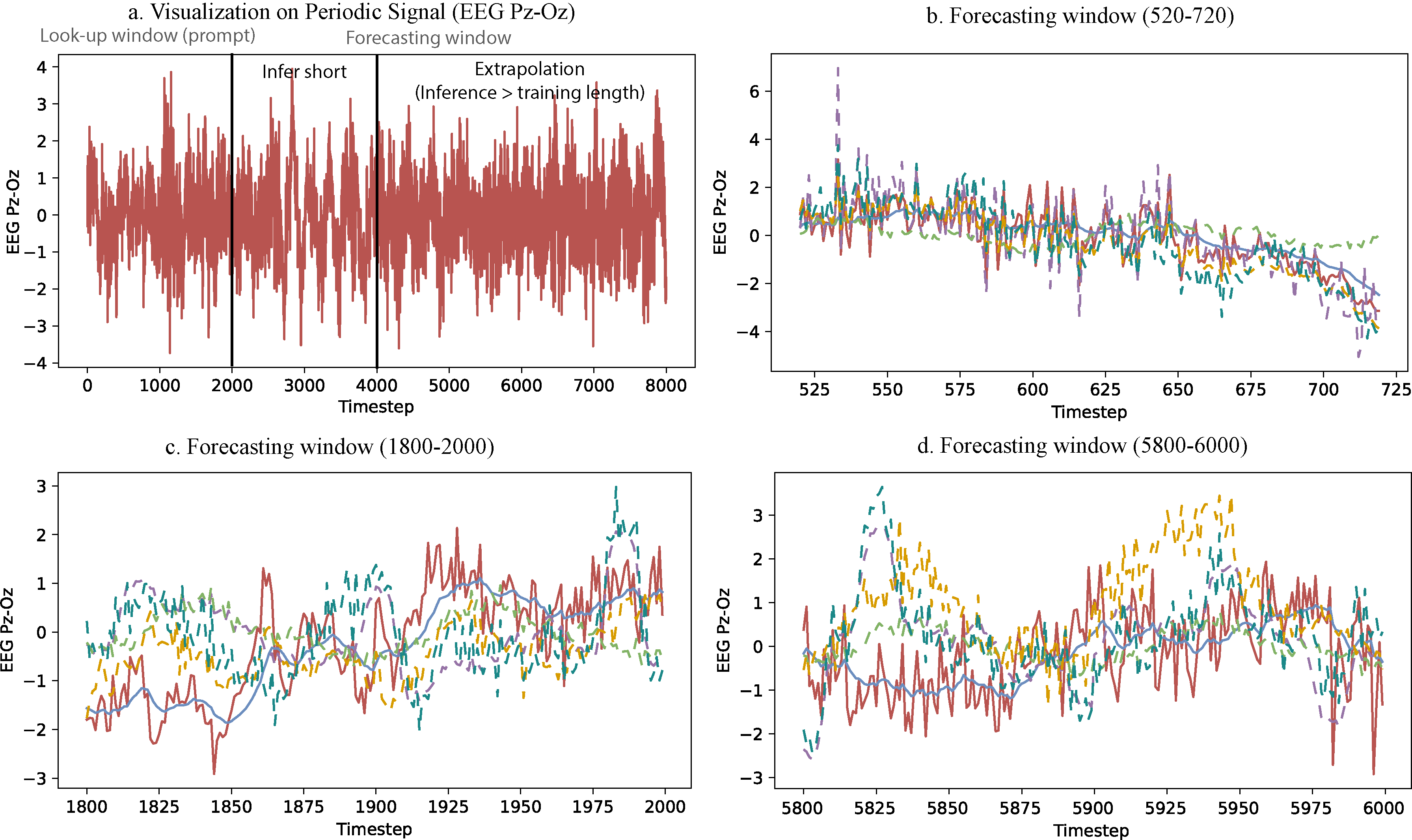
Figure 9. Example of forecasting experiments on the period signal (EEG Pz-Oz). a. the groundtruth of EEG Pz-Oz singal. The remaining panels indicate the varied forecasting windows.

Table 7. Comparison of TimelyGPT as well as 7 baselines for ultra-long-term forecasting experiment on the large-scale SleepEDF dataset.

Window Size	720	2000	6000
TimelyGPT	0.542	0.567	0.575
Informer	0.675	1.013	1.256
Autoformer	0.532	0.908	1.026
Fedformer	0.515	0.865	0.912
PatchTST	0.456	0.768	0.824
DLinear	0.521	0.840	0.929
TS2Vec	0.602	1.231	1.204
TimesNet	0.471	0.742	0.865
GPT-2 + RoPE	0.516	0.583	0.715
GPT-2	0.525	0.815	1.072

Table 8. Comparing TimelyGPT with baseline models on the downstream classification and regression tasks. Bold-faced font are the best value in each task among the 11 methods.

Task	Classification (Accuracy %)				Regression (MAE)
Pre-training	Sleep-EDF		PTB-XL		PTB-XL & PPGDalia
Fine-tuning	Sleep-EDF	Epilepsy	PTB-XL	EMG	IEEEPPG	RR	HR	SpO2
TimelyGPT	89.21	92.79	86.52	95.87	26.17	2.78	8.53	4.26
PatchTST	89.57	91.27	83.42	95.23	26.08	2.89	9.46	4.45
AutoFormer	78.86	84.21	78.51	88.56	32.18	4.13	13.29	4.95
FedFormer	76.43	81.65	75.53	85.21	31.11	4.36	13.82	4.75
TimesNet	83.58	85.96	79.38	89.26	29.95	4.19	13.65	4.83
TST	88.83	88.02	81.86	94.16	26.81	3.47	12.63	4.95
CRT	90.12	91.05	87.81	94.56	26.52	2.96	9.02	4.48
TS2Vec	86.21	88.27	82.65	93.77	27.89	3.53	11.56	4.60
TS-TCC	86.06	89.74	84.66	93.25	29.32	4.09	13.64	4.86
TF-C	86.56	87.52	82.71	93.83	28.52	4.38	14.15	4.87
LSTM	80.15	76.51	78.83	86.95	30.15	4.95	14.37	5.05

Table 9. Comparison of TimelyGPT as well as 9 baselines for multi-label classification (AUPRC %) on 12 phenotype labels.

	AMI	Asthma	CHF	COPD	Diabetes	HTN	Schizo	IHD	HIV	Epilepsy	Autism	ADHD
TimelyGPT	0.612	0.568	0.637	0.541	0.563	0.586	0.551	0.584	0.549	0.560	0.576	0.583
PatchTST	0.561	0.516	0.585	0.489	0.512	0.535	0.500	0.533	0.497	0.509	0.524	0.531
TST	0.569	0.524	0.593	0.497	0.520	0.543	0.508	0.541	0.505	0.517	0.532	0.539
CRT	0.516	0.472	0.541	0.445	0.467	0.490	0.455	0.488	0.453	0.464	0.480	0.487
TS-TCC	0.502	0.457	0.526	0.430	0.453	0.476	0.441	0.474	0.438	0.450	0.465	0.472
TS-T	0.480	0.436	0.505	0.409	0.431	0.454	0.419	0.452	0.417	0.428	0.444	0.451
mTAND	0.607	0.557	0.616	0.547	0.553	0.571	0.561	0.574	0.558	0.539	0.544	0.542
GRU-D	0.584	0.560	0.599	0.533	0.495	0.599	0.513	0.586	0.547	0.552	0.558	0.565
SeFT	0.524	0.479	0.548	0.452	0.475	0.498	0.463	0.496	0.460	0.472	0.487	0.494
RAINDROP	0.557	0.579	0.582	0.516	0.528	0.531	0.526	0.549	0.524	0.525	0.560	0.578