On the smallness conditions for a PEMFC single cell problem

Abstract.

The aim of the present paper is to prove whose smallness conditions being necessary in order to get the final result of existence of a solution. In the first part, we present the model for a proton exchange membrane fuel cell (PEMFC) single cell and we clarify the interactions of the different components namely, velocity, pressure, density, temperature and potential. The final mathematical model is a quasilinear elliptic system where the cross effects have a strong interlink. It consists of the Stokes–Darcy system altogether with thermoelectrochemical system under some non-standard interface and boundary conditions. The proof of existence of weak solutions relies on the Tychonof fixed point theorem, by providing some regularity and some smallness conditions. The actual system is divided into two systems of equations and they are separately studied. The novelty of the present work is to establish quantitative estimates for improving the technical hypotheses and, in particular, the smallness conditions in the two-dimensional case. Indeed, the smallness conditions only can be explicit if quantitative estimates are established. To this aim, we also establish quantitative estimates for the Poincaré and Sobolev inequalities and for some trilinear terms.

1. Introduction

In this paper, we present and study a model for proton exchange membrane (PEM) fuel cells, those that work at low operating temperature such as the polymer electrolyte membrane fuel cells with hydrogen supply (H₂PEMFC) and direct methanol fuel cells (DMFC). PEM fuel cells have been object of study in the last decades by their inherent energy conversion. They possess functional structure from the nanoscale up to the macroscale (see [22, 26] and the references therein) and then their descriptive models are multiscale thermoelectrochemical (TEC) systems. Numerical simulations have often been implemented in the past two decades for the study of different tasks performance [7, 10, 13, 19, 21, 28] and, in particular, for computational fluid dynamics (CFD), see [17, 30] and the references therein. Also experimental works have been performed, see [24] and the references therein. A simplified model of a self-humidifying PEM fuel cell is both numerically simulated and experimentally tested in [25].

The fuel cell consists of a membrane, two electrodes and two flow regions. The membrane is a porous medium, which is electron insulating and serves to conduct ions produced at one electrode to the other, namely the ionic charge carrier of H₃O⁺ in particular for H₂PEMFC or DMFC.

The mathematical model firstly consists of coupling of the Stokes–Fourier and Darcy–Fourier equations, known as the Stokes–Darcy–Fourier (SDF) system. We refer to [1] the study of the SDF system under both Beavers–Joseph–Saffman (BJS) and Beavers–Joseph (BJ) interface boundary conditions. The generalization of BJS-SDF problem to non-Newtonian fluids is studied in [2] by introducing the Forchheimer model. Other approach is introduced in [6], in which a nonlinear Darcy’s law is obtained by asymptotic limit of solutions to the Navier–Stokes–Fourier system in perforated domains with tiny holes, where the diameter of the holes is proportional to their mutual distance, by homogenization method.

Secondly, a thermoelectrochemical model is gathered to the Beavers–Joseph–Saffman/Stokes–Darcy problem, with some modified Butler–Volmer interface condition. The Joule effect is taken into account on the energy equation due to the electrical current. To assure that the Joule effect works better than a $L^{1}$ data, we provide some elliptic regularity for $q>n=2$ (space dimension) as it has been used in real world problems (see [8, 9] and references therein). Recently, in [11, 18] the elliptic regularity is studied and improved via the quantitative Sneiberg inequality.

Here, we do not assume that the mathematically inconvenient constants are equal to one, because the magnitude of each constant is physically relevant. Other important physical behavior is the discontinuous coefficients to allow, for instance, the viscosities being temperature dependent. This gives an extra draw back to the elliptic system. It is known that the fixed point argument is the primordial shortcoming in the existence of solutions of nonlinear PDE at the steady state and some smallness conditions are required for the application of the fixed point argument. Several hypotheses are made on the coefficients in the equations. Some of them are natural but others are technical. The reason being that the mathematical model has a strong interlink due to the cross effects. Future work should be done to improve the smallness conditions.

The outline of the present paper is as follows. Next section, we introduce the mathematical equations of the concrete physical model under consideration at the steady state. In Section 3, we state the set of hypothesis and the two-dimensional (2D) main result. Also, the physical meaning of the assumptions is discussed for a H₂-PEMFC. In Section 4, we delineate the strategy used in this paper, namely the actual system is divided into two systems of equations, which are separately studied, in order to use a fixed point argument. In order to be able to use this machinery we establish some auxiliary results in Section 5. Then, Section 6 is devoted to the existence of the two auxiliary problems, where a special care is taken in determining the quantitative estimates. Finally, Section 7 is concern to the proof of the main result.

2. Statement of the fuel cell problem

Let $\Omega$ be a bounded multidomain of $\mathbb{R}^{n}$, $n\geq 2$, that is, the domain $\Omega$ is a connected open set, which consists of different pairwise disjoint Lipschitz subdomains. Precisely, it is separated into five regions, ${\Omega}_{\mathrm{fuel}}$, ${\Omega}_{\mathrm{a}}$, ${\Omega}_{\mathrm{m}}$, ${\Omega}_{\mathrm{c}}$ and ${\Omega}_{\mathrm{air}}$, with total width $W=2l_{f}+2l_{a}+l_{m}$. The multidomain $\Omega$ represents one single PEM fuel cell, which its 2D ($xy$ cross-section) representation is schematically illustrated in Figure 1. Moreover, it has the membrane interface $\Gamma_{\mathrm{CL}}=\Gamma_{\mathrm{a}}\cup\Gamma_{\mathrm{c}}$ and the porous-fluid boundary $\Gamma$, of $(n-1)$-dimensional Lebesgue measure.

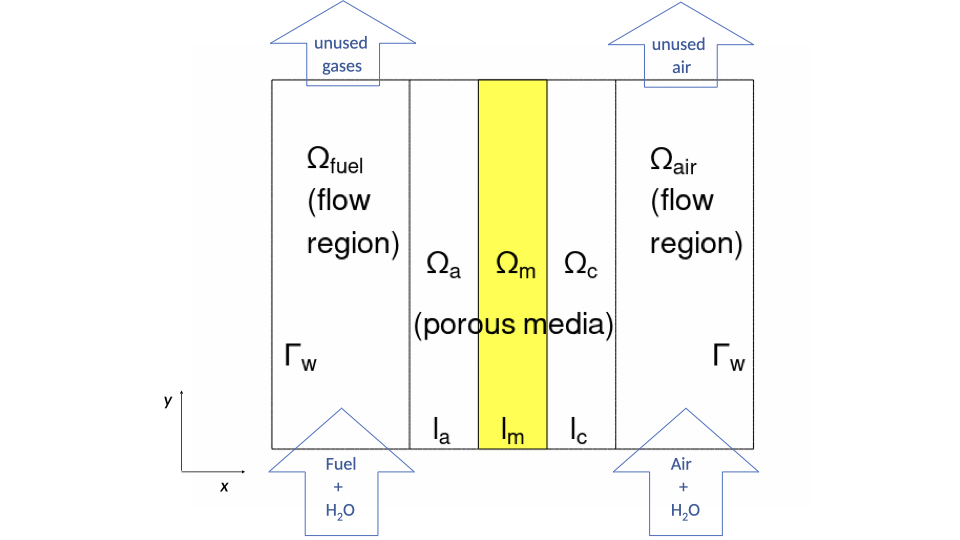
Figure 1. The flow region $\Omega_{\mathrm{f}}=\Omega_{\mathrm{fuel}}\cup\Omega_{\mathrm{air}}$ and the porous region $\Omega_{\mathrm{p}}=\Omega_{\mathrm{a}}\cup\overline{\Omega}_{\mathrm{m}}\cup\Omega_{\mathrm{c}}$ (not in scale), with width $l_{\mathrm{a}}+l_{\mathrm{m}}+l_{\mathrm{c}}<<L$ where $L=1-10\,$\mathrm{cm}$$ denotes each channel length.

We call by the fluid bidomain ${\Omega}_{\mathrm{f}}$ the two channels, namely the anodic fuel channel $\Omega_{\mathrm{fuel}}$ and the cathodic air channel $\Omega_{\mathrm{air}}$. Each channel has a typical characteristic length $l_{f}=$0.001\text{\,}\mathrm{m}$$ [14, 30].

We call by the porous domain ${\Omega}_{\mathrm{p}}$ the proton conducting membrane $\Omega_{\mathrm{m}}$, the anode and cathode backing layers, ${\Omega}_{\mathrm{a}}$ and ${\Omega}_{\mathrm{c}}$, and the anode and cathode catalyst layers (CL), $\Gamma_{\mathrm{a}}$ and $\Gamma_{\mathrm{c}}$, respectively. The backing layers are porous gas diffusion layers (GDL), with fuel in the anodic compartment and air in the cathodic compartment,where the traveling of the free electrons occurs and a current collector $\Gamma_{\mathrm{cc}}$ is attained. The catalyst layers have negligible measure when compared with the backing layers (the backing layers are approximately $l_{a}=l_{c}=$200\text{\,}\mathrm{\SIUnitSymbolMicro m}$$ in thickness, while the catalyst layers are $5\text{\,}\mathrm{\SIUnitSymbolMicro m}10\text{\,}\mathrm{\SIUnitSymbolMicro m}$ [14, 30]), and then they are assumed to be interfaces between the membrane separator and the backing layers. Hereafter, the subscripts, a and c, stand for anode and cathode, respectively.

The porous-fluid boundary is the interface $\Gamma=\partial\Omega_{\mathrm{f}}\cap\Omega=\partial\Omega_{\mathrm{p}}\cap\Omega$.

2.1. In the fluid bidomain ${\Omega}_{\mathrm{f}}=\Omega_{\mathrm{fuel}}\cup\Omega_{\mathrm{air}}$

By the characteristics of the channels, the convection for fluid and heat flows may be neglected.

The governing equations are the conservation of mass, momentum, species and energy, a.e. in $\Omega_{\mathrm{f}}$,

$$\nabla\cdot(\rho\mathbf{u})=0;$$ (2.1)

$$\nabla\cdot\tau=\nabla p;$$ (2.2)

$$\nabla\cdot(\mathbf{u}\rho_{i})+\nabla\cdot\mathbf{j}_{i}=0;$$ (2.3)

$$\nabla\cdot\mathbf{q}=0,$$ (2.4)

for the uncharged species $i=1,\cdots,\mathrm{I}$. The unknown functions are the density $\rho$, the velocity $\mathbf{u}=(u_{x},u_{y},u_{z})$, the mass concentration vector $\bm{\rho}=(\rho_{1},\cdots,\rho_{\mathrm{I}})$ and the temperature $\theta$. Each partial density is defined by

$$\rho_{i}=M_{i}c_{i},$$ (2.5)

where $M_{i}$ denotes the molar mass [$\mathrm{kg}\text{\,}{\mathrm{mol}}^{-1}$] and $c_{i}$ is the molar concentration [$\mathrm{mol}\text{\,}{\mathrm{m}}^{-3}$] of the species $i$. The following values are known: $M(\mathrm{H}_{2}\mathrm{O})=$18\text{\,}\mathrm{g}\text{\,}{\mathrm{mol}}^{-1}$$, $M(\mathrm{O}_{2})=$32\text{\,}\mathrm{g}\text{\,}{\mathrm{mol}}^{-1}$$ and $M(\mathrm{H}_{3}\mathrm{O}^{+})=$1\text{\,}\mathrm{g}\text{\,}{\mathrm{mol}}^{-1}$$. For the H₂PEMFC, $M(\mathrm{H}_{2})=$2\text{\,}\mathrm{g}\text{\,}{\mathrm{mol}}^{-1}$$, while for DMFC, $M(\mathrm{CH}_{4}\mathrm{O})=$32\text{\,}\mathrm{g}\text{\,}{\mathrm{mol}}^{-1}$$.

The deviatoric stress tensor $\tau$, which is temperature dependent, obeys the constitutive law

$$\tau=\mu(\theta)D\mathbf{u}+\lambda(\theta)\mathrm{tr}(D\mathbf{u})\mathsf{I},\qquad\mathrm{tr}(D\mathbf{u})=\mathsf{I}\mathrel{\mathop{\mathchar 58\relax}}D\mathbf{u}=\nabla\cdot\mathbf{u},$$ (2.6)

where $D=(\nabla+\nabla^{T})/2$ denotes the symmetric gradient and $\mathsf{I}$ denotes the identity ($n\times n$)-matrix. The viscosity coefficients $\mu$ and $\lambda$ are in accordance with the second law of thermodynamics

$$\mu(\theta)>0,\quad\nu(\theta)\mathrel{\mathop{\mathchar 58\relax}}=\lambda(\theta)+\mu(\theta)/n\geq 0,$$ (2.7)

with $\nu$ denoting the bulk (or volume) viscosity and $\mu/2$ being the shear (or dynamic) viscosity. Taking into account the convention on implicit summation over repeated indices, we denote $\zeta\mathrel{\mathop{\mathchar 58\relax}}\varsigma=\zeta_{ij}\varsigma_{ij}$.

We assume that the anode and cathode gas mixtures with water vapor act as ideal gases [14], that is, the pressure $p$ obeys the Boyle–Marriotte law

$$p=R_{M}\rho\theta,$$ (2.8)

where $R_{M}=R/M$ with $M$ denoting the molar mass [$\mathrm{kg}\text{\,}{\mathrm{mol}}^{-1}$].

The phenomenological fluxes, $\mathbf{j}_{i}$ [$\mathrm{kg}\text{\,}{\mathrm{s}}^{-1}\text{\,}{\mathrm{m}}^{-2}$] and $\mathbf{q}$ [$\mathrm{W}\text{\,}{\mathrm{m}}^{-2}$], are explicitly driven by

$$\mathbf{j}_{i} =-D_{i}(\theta)\nabla\rho_{i}-\sum_{\genfrac{}{}{0.0pt}{2}{j=1}{j\not={i}}}^{\mathrm{I}}D_{{i}j}(\theta)\nabla\rho_{j}-\rho_{i}S_{i}(c_{i},\theta)\nabla\theta;$$ (2.9)

$$\mathbf{q} =-R\theta^{2}\sum_{j=1}^{\mathrm{I}}D^{\prime}_{j}(c_{j},\theta)\nabla c_{j}-k(\theta)\nabla\theta,$$ (2.10)

with $i=1,\cdots,\mathrm{I}$, see [3] and the references therein. These include the Fick law (with the diffusion coefficient $D_{i}$ [${\mathrm{m}}^{2}\text{\,}{\mathrm{s}}^{-1}$]), the Fourier law (with the thermal conductivity $k$ [$\mathrm{W}\text{\,}{\mathrm{m}}^{-1}\text{\,}{\mathrm{K}}^{-1}$]), and the Dufour–Soret cross effect (with the Dufour coefficient $D^{\prime}_{i}$ [${\mathrm{m}}^{2}\text{\,}{\mathrm{s}}^{-1}\text{\,}{\mathrm{K}}^{-1}$] and the Soret coefficient $S_{i}$ [${\mathrm{m}}^{2}\text{\,}{\mathrm{s}}^{-1}\text{\,}{\mathrm{K}}^{-1}$]). While in binary liquid mixtures the Dufour effect is negligible, in binary gas mixtures the Dufour effect can be significant [12]. The universal constant is the so-called the gas constant $R=$8.314\text{\,}\mathrm{J}\text{\,}{\mathrm{mol}}^{-1}\text{\,}{\mathrm{K}}^{-1}$$.

Hereafter the subscript $i$ stands for the correspondence to the ionic component $i=1,\cdots,\mathrm{I}$ intervened in the reaction process, with $\mathrm{I}\in\mathbb{N}$ being either $\mathrm{I}_{\mathrm{p}}$ whenever $\Omega_{\mathrm{p}}$ or $\mathrm{I}_{\mathrm{f}}$ whenever $\Omega_{\mathrm{f}}$. For the sake of simplicity, we consider the number of species $\mathrm{I}=\mathrm{I}_{\mathrm{a}}=\mathrm{I}_{\mathrm{m}}=\mathrm{I}_{\mathrm{c}}=2$ (cf. Table 1).

$i$	$\Omega_{\mathrm{fuel}}\cup\Omega_{\mathrm{a}}$	$\Omega_{\mathrm{m}}$	$\Omega_{\mathrm{air}}\cup\Omega_{\mathrm{c}}$
1	fuel	H3O+	O2
2	H2O	H2O	H2O

Table 1. The correspondence of each component to each region

The water is present in fluid and vapor states, and in both cases it can be modeled as a Newtonian fluid (linearly viscous fluid).

2.2. In the porous domain $\Omega_{\mathrm{p}}=\Omega_{\mathrm{a}}\cup\overline{\Omega}_{\mathrm{m}}\cup\Omega_{\mathrm{c}}$

The governing equations, after a volume averaging procedure, are

$$\nabla\cdot\mathbf{u}_{\mathrm{D}} =0;$$ (2.11)

$$\nabla\cdot\mathbf{j}_{i} =0;$$ (2.12)

$$\nabla\cdot\mathbf{q} =Q,\mbox{ a.e. in }\Omega_{\mathrm{a}}\cup\Omega_{\mathrm{m}}\cup\Omega_{\mathrm{c}},$$ (2.13)

for $i=1,2$ and $\mathrm{I}=2$, according to Table 1. Here, it is omitted the bracket $\langle\cdot\rangle$, which usually represents the volume averaged. Thus, the temperature $\theta$ is the spatially averaged (over a representative elementary volume) microscopic quantity, and the Darcy velocity $\mathbf{u}_{\mathrm{D}}$ [$\mathrm{m}\text{\,}{\mathrm{s}}^{-1}$] is the superficial average quantity.

The volume averaged density $\rho$ of the fluid is piecewise constant, $\rho_{\mathrm{water}}=$970\text{\,}\mathrm{kg}\text{\,}{\mathrm{m}}^{-3}$$ in $\Omega_{\mathrm{m}}$ and $\rho_{\mathrm{air}}=$0.995\text{\,}\mathrm{kg}\text{\,}{\mathrm{m}}^{-3}$$ in $\Omega_{\mathrm{a}}\cup\Omega_{\mathrm{c}}$, due to $\rho_{\mathrm{air}}=p_{\mathrm{atm}}M_{\mathrm{air}}/(R\theta_{r})$, at the typical operating temperature of $\theta_{r}=$357.15\text{\,}\mathrm{K}$$ (= $84\text{\,}\mathrm{\SIUnitSymbolCelsius}$), $p_{\mathrm{atm}}=$101.325\text{\,}\mathrm{kPa}$$ and $M_{\mathrm{air}}=$28.97\text{\,}\mathrm{g}\text{\,}{\mathrm{mol}}^{-1}$$.

The Darcy velocity $\mathbf{u}_{\mathrm{D}}$ obeys

$$\mu\mathbf{u}_{\mathrm{D}}=-K_{g}\nabla p$$ (2.14)

where $p$ is the intrinsic average pressure [$\mathrm{Pa}$] and $\mu=\mu(\theta)$ denotes the viscosity [$\mathrm{Pa}\text{\,}\mathrm{s}$]. In the Darcy equation (2.14), the gravity is neglected and $K_{g}$ represents the gas permeability [${\mathrm{m}}^{2}$]. It is known that the gas permeability depends on the fiber diameter, and the Carman–Kozeny equation is commonly used [26]. The permeability should include Klinkenberg effect due to the behavior of gas flow in porous media, i.e. it obeys the Klinkenberg equation

$$K_{g}=K_{l}\left(1+\frac{b}{p}\right).$$ (2.15)

The Klinkenberg correction $b>0$ in $\Omega_{\mathrm{a}}\cup\Omega_{\mathrm{c}}$ depends on space and temperature through the porosity, $b=0$ in $\Omega_{\mathrm{m}}$, and $K_{l}>0$ being the liquid permeability of the porous media that only depends on the porosity. Therefore, $b\geq 0$ and $K_{l}$ are constant.

The phenomenological fluxes, $\mathbf{j}_{i}$ [$\mathrm{kg}\text{\,}{\mathrm{s}}^{-1}\text{\,}{\mathrm{m}}^{-2}$] and $\mathbf{q}$ [$\mathrm{W}\text{\,}{\mathrm{m}}^{-2}$], are explicitly driven by

$$\mathbf{j}_{i} =-D_{i}(\theta)\nabla\rho_{i}-D_{{i}j}(\theta)\nabla\rho_{j}-\rho_{i}S_{i}(c_{i},\theta)\nabla\theta-u_{i}\rho_{i}\nabla\phi;$$ (2.16)

$$\mathbf{q} =-R\theta^{2}\sum_{j=1}^{2}D^{\prime}_{j}(c_{j},\theta)\nabla c_{j}-k(\theta)\nabla\theta-\Pi(\theta)\sigma(\mathbf{c},\theta)\nabla\phi,$$ (2.17)

with $i,j=1,2$, and $j\not=i$. The phenomenological fluxes are explicitly driven by the gradients of the temperature $\theta$ and the mass concentration vector $\bm{\rho}$, in the form (up to some temperature and concentration dependent factors) as in (2.9)-(2.10), altogether by the gradient of the electric potential $\phi$, by incorporating the Peltier–Seebeck cross effect. We remind that the Peltier coefficient $\Pi$ [$\mathrm{V}$] and the Seebeck coefficient $\alpha_{\mathrm{S}}$ [$\mathrm{V}\text{\,}{\mathrm{K}}^{-1}$] are correlated by the first Kelvin relation

$$\Pi(\theta)=\theta\alpha_{\mathrm{S}}(\theta).$$ (2.18)

For the ionic component $i=$ H₃O⁺, the proton flux $\mathbf{J}_{i}=\mathbf{j}_{i}/M_{i}$ [$\mathrm{mol}\text{\,}{\mathrm{s}}^{-1}\text{\,}{\mathrm{m}}^{-2}$] obeys (2.16) in $\Omega_{\mathrm{m}}$, where in the first term $D_{i}=\kappa/(z_{i}F)$, with the proton ionic conductivity $\kappa$ being no constant in accordance with the membrane did not being fully hydrated. The universal constant is the so-called Faraday constant $F=$9.6485\text{\times}{10}^{4}\text{\,}\mathrm{C}\text{\,}{\mathrm{mol}}^{-1}$$.

For the dissolved water $i=$ H₂O, the molar flux $\mathbf{J}_{i}$ obeys (2.16) in $\Omega_{\mathrm{m}}$, where the second term means the electro-osmosis ($j\not=i$), with $D_{ij}=n_{\mathrm{d}}$ representing the electro-osmostic drag coefficient [14]. Moreover, $z_{\mathrm{H}_{2}\mathrm{O}}=0$ and $u_{2}=0$.

The Darcy velocity as a drift velocity does not have the relevance as in (2.3), and the drift term may be neglected in (2.12). Indeed, the drift velocity appears in the last term in (2.16) as

$$u_{i}\mathbf{E}\quad(\mathbf{E}=-\nabla\phi),$$

where $\mathbf{E}$ stands for electric field strength in $\Omega_{\mathrm{m}}$ and the ionic mobility $u_{i}$ [${\mathrm{m}}^{2}\text{\,}{\mathrm{s}}^{-1}\text{\,}{\mathrm{V}}^{-1}$] satisfies the Nernst–Einstein relation

$$u_{i}=|z_{i}|FD_{i}/(R\theta)=\kappa(\theta)/(R\theta),$$ (2.19)

which does not vanish for the valence of species $z_{\mathrm{H}^{+}}=1$.

In the energy equation (2.13), the Joule effect

$$Q=\chi_{\Omega_{\mathrm{a}}\cup\Omega_{\mathrm{c}}}\sigma(\mathbf{c},\theta)|\nabla\phi|^{2}$$ (2.20)

takes into account that the effect of flow velocity is negligible when compared to the electrical current that exists in $\Omega_{\mathrm{a}}\cup\Omega_{\mathrm{c}}$.

The electric current density $\mathbf{j}$ [$\mathrm{A}\text{\,}{\mathrm{m}}^{-2}$] is given by the Ohm law (with the electrical conductivity $\sigma$ [$\mathrm{S}\text{\,}{\mathrm{m}}^{-1}$])

$$\mathbf{j}=-\sigma(\mathbf{c},\theta)\nabla\phi\quad\mbox{ in }\Omega_{\mathrm{a}}\cup\Omega_{\mathrm{c}},$$ (2.21)

and it verifies

$$\nabla\cdot\mathbf{j}=0\quad\mbox{ a.e. in }\Omega_{\mathrm{a}}\cup\Omega_{\mathrm{c}}.$$ (2.22)

In the fuel cell model, the electric potential is given at the membrane interface (cf. Subsection 2.5). Notice that there is no electric current density in $\Omega_{\mathrm{m}}$, i.e. the electric flux $\mathbf{j}$ is the ionic current density $\mathbf{j}_{\mathrm{m}}$ that verifies $\mathbf{j}_{\mathrm{m}}=z_{\mathrm{H}^{+}}F\mathbf{J}_{\mathrm{H}^{+}}$. In practice, the flow indeed obeys the constitutive law

$$\mathbf{j}_{m}=-\kappa(\theta)\nabla\rho_{1}/M_{1}-\alpha_{\mathrm{S}}(\theta)\sigma_{m}(\rho_{2},\theta)\nabla\theta-\sigma_{m}(\rho_{2},\theta)\nabla\phi,$$ (2.23)

where the parameters are well determined. For instance, the proton conductivity $\sigma_{m}$ [$\mathrm{S}\text{\,}{\mathrm{m}}^{-1}$] may be water content and temperature dependent in contrast with the ionomer Nafion constant assumed in [4].

2.3. On the outer boundary $\partial\Omega$

The boundary of $\Omega$ is constituted by three pairwise disjoint open $(n-1)$-dimensional sets, namely $\Gamma_{\mathrm{in}}$, $\Gamma_{\mathrm{out}}$ and $\Gamma_{\mathrm{w}}$ which represent the inlet, outlet and wall boundaries, respectively,

$$\partial\Omega=\Gamma_{\mathrm{in}}\cup\Gamma_{\mathrm{out}}\cup\overline{\Gamma}_{\mathrm{w}}.$$

The wall boundary has a subpart $\Gamma_{\mathrm{cc}}\subset\partial\Omega_{\mathrm{p}}$ that stands for the current collector, meaning that the remaining wall boundary is electrical current insulated. The inlet and outlet sets are the union of two disjoint connected open $(n-1)$-dimensional sets, namely,

$$\Gamma_{\mathrm{in}} =\Gamma_{\mathrm{in,a}}\cup\Gamma_{\mathrm{in,c}};$$

$$\Gamma_{\mathrm{out}} =\Gamma_{\mathrm{out,a}}\cup\Gamma_{\mathrm{out,c}},$$

corresponding to the anodic and cathodic channels, $\Omega_{\mathrm{fuel}}$ and $\Omega_{\mathrm{air}}$ (cf. Figure 1).

On the wall boundary $\Gamma_{\mathrm{w}}$, the no outflow boundary conditions are considered to the velocity and the species,

$$\mathbf{u}\cdot\mathbf{n}=(\rho_{i}\mathbf{u}+\mathbf{j}_{i})\cdot\mathbf{n}=0\quad(i=1,\cdots,\mathrm{I}).$$ (2.24)

Hereafter, $\mathbf{n}$ denotes the outward unit normal to $\partial\Omega$.

On the inlet and outlet boundaries $\Gamma_{\mathrm{in}}\cup\Gamma_{\mathrm{out}}$, the velocity, the partial densities and the temperature are specified. Due to the characteristics of the domain, the inlet velocity is constantly specified on the $y$ direction.

• for a.e. $(x,0,z)\in\Gamma_{\mathrm{in}}$:

  $$\mathbf{u}(x,0,z) =u_{\mathrm{in}}\mathbf{e}_{y}\equiv(0,u_{\mathrm{in}},0);$$

  $$\rho_{i}(x,0,z) =\rho_{i,\mathrm{in}};$$

  $$\theta(x,0,z) =\theta_{\mathrm{in}}.$$

• for a.e. $(x,L,z)\in\Gamma_{\mathrm{out}}$:

  $$\mathbf{u}(x,L,z) =\mathbf{u}_{\mathrm{out}};$$

  $$\rho_{i}(x,L,z) =\rho_{i,\mathrm{out}};$$

  $$\theta(x,L,z) =\theta_{\mathrm{out}}.$$

We refer to [4], in where the homogeneous Dirichlet condition is assumed, whenever the general case for prescribed partial densities and temperature can be handled by subtracting background profile that fits the specified functions.

On the current collector wall boundary $\Gamma_{\mathrm{cc}}$, the electric potential is prescribed through the cell voltage $E_{\mathrm{cell}}=\phi|_{\Gamma_{\mathrm{cc,c}}}-\phi|_{\Gamma_{\mathrm{cc,a}}}$, that means

$$\phi=E_{\mathrm{cell}}\mbox{ on }\Gamma_{\mathrm{cc,c}}\quad\mbox{and}\quad\phi=0\mbox{ on }\Gamma_{\mathrm{cc,a}}.$$ (2.25)

This reflects the movement of the electrons in the GDLs, namely $\Omega_{\mathrm{a}}\cup\Omega_{\mathrm{c}}$, in the negative $x$ direction. Although the fuel reactions release approximately 1.5 joules per coulomb of electronic charge transferred and thus can be assigned a potential of $1.5\text{\,}\mathrm{V}$ [22], $E_{\mathrm{cell}}$ is known to around $0.9\text{\,}\mathrm{V}$ [27].

On the remaining wall boundary $\Gamma_{\mathrm{w}}\setminus\Gamma_{\mathrm{cc}}$, the no outflow $\mathbf{j}\cdot\mathbf{n}=0$ is considered.

Finally, the Newton law of cooling, which is mathematically known as the Robin-type boundary condition, is considered

$$\mathbf{q}\cdot\mathbf{n}=h_{c}(\theta)(\theta-\theta_{e})\mbox{ on }\Gamma_{\mathrm{w}},$$ (2.26)

where $h_{c}$ denotes the conductive heat transfer coefficient, which may depend both on the spatial variable and the temperature function $\theta$, and $\theta_{e}$ denotes the external coolant stream temperature at the wall.

2.4. On the fluid-porous interface $\Gamma$

The unit outward normal $\mathbf{n}$ to the interface boundary $\Gamma$ pointing from the fluid region to the porous medium is $\mathbf{e}_{x}$ on int$\left(\partial\Omega_{\mathrm{fuel}}\cap\partial\Omega_{\mathrm{a}}\right)$ and $-\mathbf{e}_{x}$ on int$\left(\partial\Omega_{\mathrm{air}}\cap\partial\Omega_{\mathrm{c}}\right)$.

We consider the continuity of mass flux, a constant interface temperature, and the balance of normal Cauchy stress vectors (namely, $\sigma_{fN}+\sigma_{pN}=0$)

$$\mathbf{u}\cdot\mathbf{e}_{x} =\mathbf{u}_{\mathrm{D}}\cdot\mathbf{e}_{x};$$ (2.27)

$$\theta_{\mathrm{f}} =\theta_{\mathrm{p}};$$ (2.28)

$$(\tau\cdot\mathbf{e}_{x})\cdot\mathbf{e}_{x} =[p]\mathrel{\mathop{\mathchar 58\relax}}=p_{\mathrm{f}}-p_{\mathrm{p}},$$ (2.29)

where $[\cdot]$ denotes the jump of a quantity across the interface in direction to the fluid medium. The condition (2.27) guarantees that the exchange of fluid between the two domains is conservative.

We assume the fluid flow is almost parallel to the interface and the Darcy velocity is much smaller than the slip velocity. Thus, the Beavers–Joseph–Saffman (BJS) interface boundary condition may be considered [10]

$$(\tau\cdot\mathbf{n})\cdot\mathbf{e}_{j}=-\beta\mathbf{u}\cdot\mathbf{e}_{j}\qquad(j=y,z)$$ (2.30)

where the coefficient $\beta=\alpha_{BJ}K^{-1/2}>0$ denotes the Beavers–Joseph slip coefficient, with $\alpha_{BJ}$ being dimensionless and characterizing the nature of the porous surface.

The heat transfer transmission is completed by the continuous heat flux condition

$$\mathbf{q}_{\mathrm{f}}\cdot\mathbf{e}_{x}=-\mathbf{q}_{\mathrm{p}}\cdot\mathbf{e}_{x}.$$ (2.31)

Finally, the potential is assumed to be neglected

$$\phi=0\mbox{ on }\Gamma\cap\partial\Omega_{\mathrm{a}},$$ (2.32)

while on $\Gamma\cap\partial\Omega_{\mathrm{c}}$ it is simply assumed $\nabla\phi\cdot\mathbf{n}=-\partial_{x}\phi=0$.

2.5. On the membrane interface $\Gamma_{\mathrm{CL}}=\Gamma_{\mathrm{a}}\cup\Gamma_{\mathrm{c}}$

The unit outward normal $\mathbf{n}$ to the interface boundary $\Gamma_{\mathrm{CL}}$ pointing from the backing layers to the proton conducting membrane is $\mathbf{e}_{x}$ on $\Gamma_{\mathrm{a}}$ and $-\mathbf{e}_{x}$ on $\Gamma_{\mathrm{c}}$.

The overall balanced cell reactions are

H₂PEMFC:

$2\mathrm{H}_{2}+\mathrm{O}_{2}\rightarrow 2\mathrm{H}_{2}\mathrm{O}$, $E^{0}_{\mathrm{cell}}=$1.23\text{\,}\mathrm{V}$;$

DMFC:

$2\mathrm{CH}_{4}\mathrm{O}+3\mathrm{O}_{2}\rightarrow 2\mathrm{CO}_{2}+4\mathrm{H}_{2}\mathrm{O},$ $E^{0}_{\mathrm{cell}}=$1.21\text{\,}\mathrm{V}$,$

which are the sum of two electrochemical reactions (so called half cell reactions) that occur at the electrodes.

On $\Gamma_{\mathrm{a}}=\partial\Omega_{\mathrm{a}}\cap\overline{\Omega}_{\mathrm{m}}$, it occurs the oxidation reaction of the fuel, that is,

$$\mathbf{j}_{1}\cdot\mathbf{e}_{x}=-\frac{s_{1}M(\mathrm{fuel})}{nF}j_{a}\quad\mbox{ a.e. on }\Gamma_{\mathrm{a}},$$

where $n$ stands for the number of electrons that participate in the half cell reaction and $s_{1}$ is the anodic stoichiometry number.

On $\Gamma_{\mathrm{c}}=\partial\Omega_{\mathrm{c}}\cap\overline{\Omega}_{\mathrm{m}}$, it occurs the oxygen reduction reaction, that is,

$$\mathbf{j}_{1}\cdot\mathbf{e}_{x}=-\frac{s_{1}M(\mathrm{O}_{2})}{nF}j_{c}\quad\mbox{ a.e. on }\Gamma_{\mathrm{c}},$$

with the cathodic stoichiometry number $s_{1}$.

Thus, the electric current may be modeled by

$$\mathbf{j}\cdot\mathbf{n}=j_{\ell}(\eta_{\ell})\quad\mbox{ a.e. on }\Gamma_{\ell},\quad(\ell=\mathrm{a,c}),$$ (2.33)

where the reaction rates $j_{\ell}$ [$\mathrm{A}\text{\,}{\mathrm{m}}^{-2}$] are given by

$$j_{\ell}(\eta)=\left\{\begin{array}[]{ll}j_{\ell,L}\frac{2j_{\ell,0}\sinh[\eta/B_{\ell}]}{j_{\ell,L}+2j_{\ell,0}\sinh[\eta/B_{\ell}]}&\quad\mbox{ if }\eta\geq 0\\ -j_{\ell}(-\eta)&\quad\mbox{ if }\eta<0\end{array}\right.$$ (2.34)

with $B_{\ell}=R\theta_{\ell}/F$ being the Tafel slope at $\ell=a,c$, for some reference temperatures $\theta_{a}$ and $\theta_{c}$. Here, it is considered that $\eta_{\ell}=\phi_{\ell}-\phi_{m}-\phi_{r}$ stands for the overpotential ($\ell=a,c$), for some reference potential $\phi_{r}$, the limiting current $j_{\ell,L}$, and some $j_{\ell,0}>0$ only spatial dependent being such that $j_{\mathrm{a},0}>>j_{\mathrm{c},0}$ ($j_{\mathrm{a},0}=$1800\text{\,}\mathrm{A}\text{\,}{\mathrm{m}}^{-2}$$ and $j_{\mathrm{c},0}=$0.0132\text{\,}\mathrm{A}\text{\,}{\mathrm{m}}^{-2}$$ [29]).

We emphasize that the experimental potential jumps at the interface, i.e. the anodic and the cathodic overpotentials are, respectively, $\eta_{a}<0$ and $\eta_{c}>0$. The modeling (2.33)-(2.34) avoids the existence of infinitely many non-trivial solutions that happens on the Steklov problem [20].

For the discussion of the Butler–Volmer and Bernardi–Verbrugge boundary conditions, we may refer to [5].

3. Variational formulation and main result

In the framework of Sobolev and Lebesgue functional spaces, for $r>1$, we introduce the following spaces of test functions

$$\mathbf{V}(\Omega_{f})= \{\mathbf{v}\in\mathbf{H}^{1}(\Omega_{\mathrm{f}})\mathrel{\mathop{\mathchar 58\relax}}\ \mathbf{v}=\mathbf{0}\mbox{ on }\Gamma_{\mathrm{in}}\cup\Gamma_{\mathrm{out}};\ \mathbf{v}\cdot\mathbf{n}=0\mbox{ on }\Gamma_{\mathrm{w}}\};$$

$$H(\Omega_{p})= \{v\in L^{2}(\Omega_{\mathrm{p}})\mathrel{\mathop{\mathchar 58\relax}}\ v_{a}\mathrel{\mathop{\mathchar 58\relax}}=v|_{\Omega_{\mathrm{a}}}\in H^{1}(\Omega_{\mathrm{a}}),\ v_{c}\mathrel{\mathop{\mathchar 58\relax}}=v|_{\Omega_{\mathrm{c}}}\in H^{1}(\Omega_{\mathrm{c}}),$$

$$\ v_{m}\mathrel{\mathop{\mathchar 58\relax}}=v|_{\Omega_{\mathrm{m}}}\in H^{1}(\Omega_{\mathrm{m}}),\ v_{a}=v_{m}\mbox{ on }\Gamma_{\mathrm{a}},\ v_{c}=v_{m}\mbox{ on }\Gamma_{\mathrm{c}}\};$$

$$V(\Omega)= \{v\in L^{2}(\Omega)\mathrel{\mathop{\mathchar 58\relax}}\ v_{\ell}\mathrel{\mathop{\mathchar 58\relax}}=v|_{\Omega_{\ell}}\in H^{1}(\Omega_{\ell}),\ \ell=\mathrm{a},\mathrm{c},\mathrm{f},\ v_{m}\mathrel{\mathop{\mathchar 58\relax}}=v|_{\Omega_{\mathrm{m}}}\in H^{1}(\Omega_{\mathrm{m}}),$$

$$\ v_{\ell}=v_{m}\mbox{ on }\Gamma,\ \ell=\mathrm{a},\mathrm{c},\ v=0\mbox{ on }\Gamma_{\mathrm{in}}\cup\Gamma_{\mathrm{out}}\};$$

$$V(\Omega)= \{v\in H^{1}(\Omega)\mathrel{\mathop{\mathchar 58\relax}}\ v=0\mbox{ on }\Gamma_{\mathrm{in}}\cup\Gamma_{\mathrm{out}}\};$$

$$V_{r}(\Omega_{p})= \{v\in W^{1,r}(\Omega_{\mathrm{p}})\mathrel{\mathop{\mathchar 58\relax}}\ v=0\mbox{ on }\Gamma_{\mathrm{cc}}\cup(\Gamma\cap\partial\Omega_{\mathrm{a}})\};$$

$$H(\Omega)= \{v\in H^{1}(\Omega)\mathrel{\mathop{\mathchar 58\relax}}\ v_{f}\mathrel{\mathop{\mathchar 58\relax}}=v|_{\Omega_{\mathrm{f}}},\ v_{p}\mathrel{\mathop{\mathchar 58\relax}}=v|_{\Omega_{\mathrm{p}}},\ v_{f}=v_{p}\mbox{ on }\Gamma\},$$

with their usual norms. Considering that the Poincaré inequality occurs whenever the trace of the function vanishes on a part with positive measure of the boundary $\partial\Omega$, then the Hilbert spaces, $\mathbf{V}(\Omega_{f})$, $V_{2}(\Omega_{p})$ and $V(\Omega)$, are endowed with the standard seminorms (cf. Section 5). We denote $V(\Omega_{p})=V_{2}(\Omega_{p})$, for the sake of simplicity.

The fuel cell problem, which its strong formulation is stated in Section 2, is equivalent to the following variational formulation.

Definition 3.1.

We say that the function $(\mathbf{u},p,\bm{\rho},\theta,\phi)$ is a weak solution to the fuel cell problem, if it satisfies the following variational formulations to

• the momentum conservation (Beavers–Joseph–Saffman/Stokes–Darcy problem)

  $$\int_{\Omega_{\mathrm{f}}}\mu(\theta)D\mathbf{u}\mathrel{\mathop{\mathchar 58\relax}}D\mathbf{v}\operatorname{d\!}{x}+\int_{\Omega_{\mathrm{f}}}\lambda(\theta)\nabla\cdot\mathbf{u}\nabla\cdot\mathbf{v}\operatorname{d\!}{x}+\int_{\Omega_{\mathrm{p}}}\frac{K_{g}(p)}{\mu(\theta)}\nabla p\cdot\nabla v\operatorname{d\!}{x}$$

  $$+\int_{\Gamma}\beta(\theta)\mathbf{u}_{T}\cdot\mathbf{v}_{T}\operatorname{d\!}{s}+\int_{\Gamma}p\mathbf{v}\cdot\mathbf{n}\operatorname{d\!}{s}-\int_{\Gamma}\mathbf{u}\cdot\mathbf{n}v\operatorname{d\!}{s}$$

  $$=R_{M}\int_{\Omega_{\mathrm{f}}}\rho\theta\nabla\cdot\mathbf{v}\operatorname{d\!}{x},$$ (3.1)

  holds for all $(\mathbf{v},v)\in\mathbf{V}(\Omega_{f})\times H(\Omega_{p})$. Here, $\rho=\rho_{1}+\rho_{2}$.

• the species conservation ($i=1,2$)

  $$\int_{\Omega_{\mathrm{f}}}\rho_{1}\mathbf{u}\cdot\nabla v\operatorname{d\!}{x}+\int_{\Omega}D_{1}(\theta)\nabla\rho_{1}\cdot\nabla v\operatorname{d\!}{x}+\frac{F}{R}\int_{\Omega_{\mathrm{m}}}\psi(\rho_{1})\frac{D_{1}(\theta)}{\theta}\nabla\phi\cdot\nabla v\operatorname{d\!}{x}$$

  $$+\int_{\Omega_{\mathrm{m}}}D_{12}(\theta)\nabla\rho_{2}\cdot\nabla v\operatorname{d\!}{x}+\int_{\Omega}\rho_{1}S_{1}(\rho_{1},\theta)\nabla\theta\cdot\nabla v\operatorname{d\!}{x}=0;$$ (3.2)

  $$\int_{\Omega_{\mathrm{f}}}\rho_{2}\mathbf{u}\cdot\nabla v\operatorname{d\!}{x}+\int_{\Omega}D_{2}(\theta)\nabla\rho_{2}\cdot\nabla v\operatorname{d\!}{x}+\int_{\Omega_{\mathrm{m}}}n_{\mathrm{d}}(\theta)\nabla\rho_{1}\cdot\nabla v\operatorname{d\!}{x}$$

  $$+\int_{\Omega}\rho_{2}S_{2}(\rho_{2},\theta)\nabla\theta\cdot\nabla v\operatorname{d\!}{x}=0,$$ (3.3)

  holds for all $v\in V(\Omega)$. Here, we set

  $$\psi(z)=\left\{\begin{array}[]{ll}z&\mbox{ if }0\leq z\leq\rho_{1,m}\\ 0&\mbox{ otherwise}\end{array}\right.$$

  for some $\rho_{1,m}>0$.

• the energy conservation

  $$\int_{\Omega}k(\theta)\nabla\theta\cdot\nabla v\operatorname{d\!}{x}+\int_{\Gamma_{\mathrm{w}}}h_{c}(\theta)\theta v\operatorname{d\!}{s}$$

  $$+\sum_{j=1}^{2}\frac{R}{M_{j}}\int_{\Omega}\theta^{2}D_{j}^{\prime}(\rho_{j},\theta)\nabla\rho_{j}\cdot\nabla v\operatorname{d\!}{x}+\int_{\Omega_{\mathrm{m}}}\Pi(\theta)\sigma_{m}(\rho_{2},\theta)\nabla\phi\cdot\nabla v\operatorname{d\!}{x}$$

  $$=\int_{\Gamma_{\mathrm{w}}}h_{c}(\theta)\theta_{e}v\operatorname{d\!}{s}+\int_{\Omega_{\mathrm{a}}\cup\Omega_{\mathrm{c}}}\sigma(\bm{\rho},\theta)|\nabla\phi|^{2}v\operatorname{d\!}{x},$$ (3.4)

  holds for all $v\in V(\Omega)$.

• the electricity conservation

  $$\int_{\Omega_{\mathrm{p}}}\sigma(\bm{\rho},\theta)\nabla\phi\cdot\nabla w\operatorname{d\!}{x}+\frac{1}{M_{1}}\int_{\Omega_{\mathrm{m}}}\kappa(\theta)\nabla\rho_{1}\cdot\nabla w\operatorname{d\!}{x}$$

  $$+\int_{\Omega_{\mathrm{m}}}\alpha_{\mathrm{S}}(\theta)\sigma_{m}(\rho_{2},\theta)\nabla\theta\cdot\nabla w\operatorname{d\!}{x}$$

  $$+\int_{\Gamma_{\mathrm{a}}}j_{a}(\phi_{a}-\phi_{m})(w_{a}-w_{m})\operatorname{d\!}{s}+\int_{\Gamma_{\mathrm{c}}}j_{c}(\phi_{c}-\phi_{m}-E_{\mathrm{cell}})(w_{c}-w_{m})\operatorname{d\!}{s}=0,$$ (3.5)

  holds for all $w\in V(\Omega_{p})$.

Hereafter, the notation $\operatorname{d\!}{x}$ refers to the 2D $\operatorname{d\!}{x}\operatorname{d\!}{y}$ and the 3D $\operatorname{d\!}{x}\operatorname{d\!}{y}\operatorname{d\!}{z}$ and whenever this may be misunderstanding we use $\operatorname{d\!}{x_{1}}\operatorname{d\!}{x_{2}}\operatorname{d\!}{x_{3}}$. We use the notation $\operatorname{d\!}{s}$ for the surface element in the integrals on the boundary as well as any subpart of the boundary $\partial\Omega$. In (• ‣ 3.1), the subscripts denote the restriction to $\Omega_{\ell}$, $\ell=$ a, c, or $\Omega_{\mathrm{m}}$.

Remark 3.1.

The truncation $\psi$ is assumed, which is consistent with the real behavior of the partial density of H₃O⁺ in the membrane. Mathematically speaking, it avoids some extra regularity of the weak solutions and, consequently, the even more restriction on the smallness conditions. We emphasize that the $L^{\infty}$-bound of solutions of elliptic equations is not straightforward true for elliptic systems [16].

The set of hypothesis is as follows.

(H1):

The viscosities $\mu$ and $\lambda$ are assumed to be Carathéodory functions from $\Omega_{\mathrm{f}}\times\mathbb{R}$ into $\mathbb{R}$, i.e. measurable with respect to space variable and continuous with respect to other variable, such that

$$\exists\mu_{\#},\mu^{\#}>0\mathrel{\mathop{\mathchar 58\relax}} \ \mu_{\#}\leq\ \mu(x,e)\leq\mu^{\#};$$ (3.6)

$$\exists\lambda^{\#}>0\mathrel{\mathop{\mathchar 58\relax}} \ -\mu/n\leq\lambda(x,e)\leq\lambda^{\#},$$ (3.7)

for a.e. $x\in\Omega_{\mathrm{f}}$ and for all $e\in\mathbb{R}$. While $K_{g}$ is assumed to be Carathéodory function from $\Omega_{\mathrm{p}}\times\mathbb{R}$ into $\mathbb{R}$ such that

$$\exists K_{l},K_{l}^{\#}>0\mathrel{\mathop{\mathchar 58\relax}}\ K_{l}\leq K_{g}(x,e)\leq K_{l}^{\#},$$ (3.8)

for a.e. $x\in\Omega_{\mathrm{p}}$ and for all $e\in\mathbb{R}$.

(H2):

The leading coefficients $D_{i}$ and $k$ are Carathéodory functions from $\Omega\times\mathbb{R}$ to $\mathbb{R}$ and $\sigma$ is a Carathéodory function from $\Omega\times\mathbb{R}^{3}$ to $\mathbb{R}$ such that $\sigma(x,\cdot)\equiv\sigma_{m}\in C(\mathbb{R}^{2})$ for a.e $x\in\Omega_{\mathrm{m}}$. Moreover, they satisfy

$$\exists D_{i}^{\#},D_{i,\#}>0\mathrel{\mathop{\mathchar 58\relax}}\ D_{i,\#}\leq D_{i}(x,e)\leq D_{i}^{\#},\quad\mbox{ for a.e. }x\in\Omega_{\mathrm{m}}\cup\Omega_{\mathrm{GDL}};$$ (3.9)

$$\exists D_{i,m}^{\#},D_{i,m}>0\mathrel{\mathop{\mathchar 58\relax}}\ D_{1,_{m}}\leq D_{1}(x,e)\leq\left\{\begin{array}[]{ll}D_{1,m}^{\#}|e|/T^{\#}&\mbox{if }|e|\leq T^{\#}\\ D_{1,m}^{\#}&\mbox{if }|e|>T^{\#}\end{array}\right.$$ (3.12)

$$D_{2,_{m}}\leq D_{2}(x,e)\leq D_{2,m}^{\#},\quad\mbox{ for a.e. }x\in\Omega_{\mathrm{m}};$$ (3.13)

$$\exists k^{\#},k_{\#}>0\mathrel{\mathop{\mathchar 58\relax}}\ k_{\#}\leq k(x,e)\leq k^{\#},\quad\mbox{ for a.e. }x\in\Omega;$$ (3.14)

$$\exists\sigma^{\#},\sigma_{\#}>0\mathrel{\mathop{\mathchar 58\relax}}\ \sigma_{\#}\leq\sigma(x,\mathbf{e})\leq\sigma^{\#},\quad\mbox{ for a.e. }x\in\Omega_{\mathrm{a}}\cup\Omega_{\mathrm{c}};$$ (3.15)

$$\exists\sigma_{m}^{\#},\sigma_{m,\#}>0\mathrel{\mathop{\mathchar 58\relax}}\ \sigma_{m,\#}\leq\sigma_{m}(d,e)\leq\sigma_{m}^{\#},$$ (3.16)

for all $d,e\in\mathbb{R}$ and $\mathbf{e}\in\mathbb{R}^{3}$.

(H3):

The cross-effect Peltier, Seebeck, Soret, Dufour and binary diffusion coefficients $\Pi,\alpha_{\mathrm{S}},S_{i}$, $D_{i}^{\prime},D_{ij}$ ($i,j=1,2$ with $j\not=i$) are Carathéodory functions such that

$$\exists\Pi^{\#}>0\mathrel{\mathop{\mathchar 58\relax}}\ |\Pi(x,e)|\leq\Pi^{\#},\quad\mbox{ for a.e. }x\in\Omega_{\mathrm{p}};$$ (3.17)

$$\exists\alpha^{\#}>0\mathrel{\mathop{\mathchar 58\relax}}\ |\alpha_{\mathrm{S}}(x,e)|\leq\alpha^{\#},\quad\mbox{ for a.e. }x\in\Omega_{\mathrm{m}};$$ (3.18)

$$\exists S_{i}^{\#}>0\mathrel{\mathop{\mathchar 58\relax}}\ |dS_{i}(x,d,e)|\leq S_{i}^{\#},\quad\mbox{ for a.e. }x\in\Omega;$$ (3.19)

$$\exists(D_{i}^{\prime})^{\#}>0\mathrel{\mathop{\mathchar 58\relax}}\ (R/M_{i})e^{2}|D_{i}^{\prime}(x,d,e)|\leq(D_{i}^{\prime})^{\#},\quad\mbox{ for a.e. }x\in\Omega;$$ (3.20)

$$\exists D_{ij}^{\#}>0\mathrel{\mathop{\mathchar 58\relax}}\ |D_{ij}(x,e)|\leq D_{ij}^{\#},\quad\mbox{ for a.e. }x\in\Omega,$$ (3.21)

for all $d,e\in\mathbb{R}$. Moreover, we assume

$$a_{1,\#} \mathrel{\mathop{\mathchar 58\relax}}=\frac{1-\epsilon_{1}-\epsilon_{2}-\epsilon_{3}}{2}D_{1,\#}-\frac{1}{\epsilon_{6}}\frac{((D^{\prime}_{1})^{\#})^{2}}{k_{\#}}>0;$$ (3.22)

$$a_{1,m} \mathrel{\mathop{\mathchar 58\relax}}=\frac{1-\epsilon_{1}-\epsilon_{3}}{2}D_{1,m}-\frac{1}{\epsilon_{6}}\frac{((D^{\prime}_{1})^{\#})^{2}}{k_{\#}}-\frac{1}{\epsilon_{4}}\frac{(D^{\#}_{21})^{2}}{D_{2,m}}-\frac{F^{2}}{\epsilon_{8}M_{1}^{2}}\frac{(D_{1,m}^{\#})^{2}}{\sigma_{m,\#}}>0;$$ (3.23)

$$a_{2,\#} \mathrel{\mathop{\mathchar 58\relax}}=\frac{1-\epsilon_{4}-\epsilon_{5}}{2}D_{2,\#}-\frac{1}{\epsilon_{6}}\frac{((D^{\prime}_{2})^{\#})^{2}}{k_{\#}}>0;$$ (3.24)

$$a_{2,m} \mathrel{\mathop{\mathchar 58\relax}}=\frac{1-\epsilon_{4}}{2}D_{2,m}-\frac{1}{\epsilon_{6}}\frac{((D^{\prime}_{2})^{\#})^{2}}{k_{\#}}-\frac{1}{\epsilon_{1}}\frac{(D^{\#}_{12})^{2}}{D_{1,m}}>0;$$ (3.25)

$$a_{3,\#} \mathrel{\mathop{\mathchar 58\relax}}=\frac{1-\epsilon_{6}-\epsilon_{7}}{2}k_{\#}-\frac{1}{\epsilon_{2}}\frac{(S_{1}^{\#})^{2}}{D_{1,\#}}-\frac{1}{\epsilon_{5}}\frac{(S_{2}^{\#})^{2}}{D_{2,\#}}>0;$$ (3.26)

$$a_{3,m} \mathrel{\mathop{\mathchar 58\relax}}=\frac{1-\epsilon_{7}}{2}k_{\#}-\frac{1}{\epsilon_{2}}\frac{(S_{1}^{\#})^{2}}{D_{1,m}}-\frac{1}{\epsilon_{5}}\frac{(S_{2}^{\#})^{2}}{D_{2,m}}-\frac{1}{\epsilon_{9}}(\alpha^{\#})^{2}\sigma^{\#}>0;$$ (3.27)

$$a_{4,m} \mathrel{\mathop{\mathchar 58\relax}}=\sigma_{m,\#}\left(1-\frac{\epsilon_{8}+\epsilon_{9}}{2}-\frac{1}{2\epsilon_{7}}\frac{(\Pi^{\#})^{2}\sigma_{m}^{\#}}{k_{\#}}\right)-\frac{1}{2\epsilon_{3}}\frac{(\rho_{1,m}\kappa^{\#})^{2}}{D_{1,m}}>0.$$ (3.28)

for some $\epsilon_{1},\cdots,\epsilon_{9}>0$ being such that $\epsilon_{1}+\epsilon_{2}+\epsilon_{3}<1$, $\epsilon_{4}+\epsilon_{5}<1$, $\epsilon_{6}+\epsilon_{7}<1$ and $\epsilon_{8}+\epsilon_{9}<2$. Here, $\rho_{1,m}$ stands for the upper bound given at (H8) and $\kappa^{\#}\mathrel{\mathop{\mathchar 58\relax}}=FD_{1,m}^{\#}/(RT^{\#})$.

(H4):

The boundary coefficient $\beta$ is assumed to be a Carathéodory function from $\Gamma\times\mathbb{R}$ into $\mathbb{R}$. Moreover, there exist $\beta_{\#},\beta^{\#}>0$ such that

$$\beta_{\#}\leq\beta(\cdot,e)\leq\beta^{\#},$$ (3.29)

a.e. in $\Gamma$, and for all $e\in\mathbb{R}$.

(H5):

The boundary coefficient $h_{c}$ is assumed to be a Carathéodory function from $\Gamma_{\mathrm{w}}\times\mathbb{R}$ into $\mathbb{R}$. Moreover, there exist $h_{\#},h^{\#}>0$ such that

$$h_{\#}\leq h_{c}(\cdot,e)\leq h^{\#},$$ (3.30)

a.e. in $\Gamma_{\mathrm{w}}$, and for all $e\in\mathbb{R}$.

(H6):

The boundary functions $j_{\ell}$, $\ell=$ a, c, are assumed to be the increasing, odd continuous functions from $\mathbb{R}$ into $\mathbb{R}$, defined in (2.34).

(H7):

There exists $\mathbf{u}_{0}\in\mathbf{H}^{1}(\Omega_{\mathrm{f}})$ such that $\mathbf{u}_{0}=u_{\mathrm{in}}\mathbf{e}_{y}$ on $\Gamma_{\mathrm{in}}$, $\mathbf{u}_{0}=\mathbf{u}_{\mathrm{out}}$ on $\Gamma_{\mathrm{out}}$ and $\mathbf{u}_{0}=\mathbf{0}$ on $\partial\Omega_{\mathrm{f}}\setminus\left(\Gamma_{\mathrm{in}}\cup\Gamma_{\mathrm{out}}\right)$.

(H8):

There exist $\rho_{1,0}$ and $\rho_{2,0}$ belong to $C(\overline{\Omega})$ such that $\rho_{i,0}=\rho_{i,\mathrm{in}}$on $\Gamma_{\mathrm{in}}$, $\rho_{i,0}=\rho_{i,\mathrm{out}}$on $\Gamma_{\mathrm{out}}$ and $\nabla\rho_{i,0}\cdot\mathbf{n}=0$ on $\partial\Omega\setminus\left(\Gamma_{\mathrm{in}}\cup\Gamma_{\mathrm{out}}\right)$, for $i=1,2$. Moreover, the lower and upper bounds $0\leq\rho_{1,0}\leq\rho_{1,m}$ occur a.e. in $\Omega_{\mathrm{m}}$.

(H9):

There exists $\theta_{0}\in H^{1}(\Omega)$ such that $\theta_{0}=\theta_{\mathrm{in}}$on $\Gamma_{\mathrm{in}}$ and $\theta_{0}=\theta_{\mathrm{out}}$on $\Gamma_{\mathrm{out}}$.

Remark 3.2.

The nonstandard assumptions (3.22)-(3.28) are required for the Legendre–Hadamard ellipticity condition.

Using the fixed point argument, we establish the following 2D result under the smallness on the data.

Theorem 3.1.

Let $\Omega$ be a bounded multiregion domain of $\mathbb{R}^{n}$, $n=2$. Under the assumptions (H1)-(H9), the fuel cell problem admits, at least, one solution according to Definition 3.1 such that

• the velocity $\mathbf{u}\in\mathbf{u}_{0}+\mathbf{V}(\Omega_{f})$;

• the pressure $p\in H(\Omega_{p})$;

• the partial densities $\bm{\rho}\in\bm{\rho}_{0}+[V(\Omega)]^{2}$;

• the temperature $\theta\in\theta_{0}+V(\Omega)$;

• the potential $\phi\in E_{cell}\chi_{\Omega_{\mathrm{c}}}+V_{r}(\Omega_{p})$, for $r>2$,

if provided by the smallness condition

$$root_{2}>\sqrt{\frac{2C_{K}}{\mu_{\#}}}C_{0}+\sqrt{C_{K}L}\frac{R_{M}}{\mu_{\#}}\frac{1}{a_{\#}}\left(h^{\#}\|\theta_{e}\|_{2,\Gamma_{\mathrm{w}}}^{2}+2\mathcal{B}_{0}\right),$$ (3.31)

where $root_{2}$ is the positive root of the quadratic polynomial (7.4), $C_{K}>1$ is the Korn constant in (5.1) and $C_{0},\mathcal{B}_{0},a_{\#}>0$ are constants defined in (6.2), (6.7) and (7.6), respectively.

In the sequel, we focus on the H₂PEMFC. Under the operating parameters [7, 14], the following data are known.

1. The viscosities are known decreasing functions on temperature, for instance in the operating temperature range $320\text{\,}\mathrm{K}390\text{\,}\mathrm{K}$, $\mu_{\#}\approx$4.2\text{\times}{10}^{-5}\text{\,}\mathrm{Pa}\text{\,}\mathrm{s}$$ and $\mu^{\#}\approx$4.8\text{\times}{10}^{-5}\text{\,}\mathrm{Pa}\text{\,}\mathrm{s}$$ for the air. The water viscosity $\mu_{water}\approx 100\mu_{air}$.

2. For values of $K=$1.76\text{\times}{10}^{-11}\text{\,}{\mathrm{m}}^{2}$$ we have $\beta$ of order $10^{5}$. We may assume $\beta_{\#}=1$ in (H4).

3. The thermal conductivity for H₂ varies from $k_{\mathrm{H}_{2}}($300\text{\,}\mathrm{K}$)=$0.18\text{\,}\mathrm{W}\text{\,}{\mathrm{m}}^{-1}\text{\,}{\mathrm{K}}^{-1}$$ to $k_{\mathrm{H}_{2}}($400\text{\,}\mathrm{K}$)=$0.2\text{\,}\mathrm{W}\text{\,}{\mathrm{m}}^{-1}\text{\,}{\mathrm{K}}^{-1}$$. Typical values of the thermal conductivity $k\approx 0.03$, 0.023 and $0.67\text{\,}\mathrm{W}\text{\,}{\mathrm{m}}^{-1}\text{\,}{\mathrm{K}}^{-1}$ are known for air, for water vapor and for liquid water, respectively. In $\Omega_{\mathrm{p}}$, the thermal conductivity varies in the range $0.2-0.5$ $\mathrm{W}\text{\,}{\mathrm{m}}^{-1}\text{\,}{\mathrm{K}}^{-1}$. Considering the electrical conductivity $\sigma^{\#}=$120\text{\,}\mathrm{S}\text{\,}{\mathrm{m}}^{-1}$$ and Peltier coefficients with its maximum of $\Pi^{\#}=0.3$ [29], then the smallness condition (3.28) is by validated by (2.18). For the anode, we have $\alpha^{\#}=0.3/320<<(k_{\#}/\sigma^{\#})^{1/2}\approx 0.04$.

4. For air/O₂, the inlet velocity is $u_{\mathrm{in}}=$0.2\text{\,}\mathrm{m}\text{\,}{\mathrm{s}}^{-1}$$ then $1.9\lesssim\sqrt{\beta^{\#}}u_{\mathrm{in}}|\Gamma|^{1/2}\lesssim 6.3$, with $0.03\leq\sqrt{L}\leq 10^{-1}<2/(1+2\sqrt{2})\approx 0.5$.

5. The inlet concentration of hydrogen is known as around $54\text{\,}\mathrm{mol}\text{\,}{\mathrm{m}}^{-3}$. Recalling (2.5), we know $\rho_{1,\mathrm{in}}(\mathrm{H}_{2})=$0.1\text{\,}\mathrm{kg}\text{\,}{\mathrm{m}}^{-3}$>\rho_{1,m}$.

6. Typical values for diffusion coefficients are $D_{\mathrm{O}_{2}}(\theta)=1.77\times 10^{-4}(\theta/273)^{1.8}$ and $D_{\mathrm{H}_{2}\mathrm{O}}(\theta)=2.56\times 10^{-5}(\theta/307)^{2.3}$, while for hydrogen in water vapor $D_{1}\approx$9.15\text{\times}{10}^{-5}\text{\,}{\mathrm{m}}^{2}\text{\,}{\mathrm{s}}^{-1}$$. In the membrane $\Omega_{\mathrm{m}}$, the binary diffusion coefficient $D_{21}=$1.1\text{\times}{10}^{-8}\text{\,}{\mathrm{m}}^{2}\text{\,}{\mathrm{s}}^{-1}$$, while typical values of diffusion coefficients are $D_{\mathrm{O}_{2}}(\theta)=2.88\times 10^{-10}\exp\left[2933(1/313-1/\theta)\right]$, $D_{\mathrm{O}_{2}}(\theta)=4.1\times 10^{-7}\exp\left[-2602/\theta\right]$ and $D_{2}=0$ [14].

7. Heat transfer coefficients are $h_{\mathrm{H}_{2}\mathrm{O}}=$2672\text{\,}\mathrm{W}\text{\,}{\mathrm{m}}^{-2}\text{\,}{\mathrm{K}}^{-1}$$, $h_{\mathrm{H}_{2}}=$824\text{\,}\mathrm{W}\text{\,}{\mathrm{m}}^{-2}\text{\,}{\mathrm{K}}^{-1}$$ and $h_{air}=$1200\text{\,}\mathrm{W}\text{\,}{\mathrm{m}}^{-2}\text{\,}{\mathrm{K}}^{-1}$$ [23].

The method applied in determining explicit constants, namely in Proposition 5.1, does not work in 3D unless the additional assumption of the functions vanish at least on the solid wall basis ($z=0$). However, neither the fluid velocity field nor the partial densities verify the Dirichlet condition on real situations. The fluid velocity field is only known impenetrable on the solid boundary while the partial densities exist satisfying (2.24).

4. Strategy

Set the $(\bm{\rho},\theta)$-dependent $4\times 4$-matrix

$$\mathsf{A}(\bm{\rho},\theta)=\left[\begin{array}[]{cccc}D_{1}(\theta)&D_{12}(\rho_{2},\theta)&\rho_{1}S_{1}(\rho_{1},\theta)&\rho_{1}\kappa(\theta)/(R\theta)\\ D_{21}(\rho_{1},\theta)&D_{2}(\theta)&\rho_{2}S_{2}(\rho_{2},\theta)&0\\ R\theta^{2}D^{\prime}_{1}(\rho_{1},\theta)/M_{1}&R\theta^{2}D_{2}(\rho_{2},\theta)/M_{2}&k(\theta)&\Pi(\theta)\sigma_{m}(\theta)\\ \kappa(\theta)/M_{1}&0&\alpha_{S}(\theta)\sigma_{m}(\theta)&\sigma(\bm{\rho},\theta)\end{array}\right].$$

The existence of the weak solution to the fuel cell problem relies on the fixed point argument

$$\mathcal{T}\mathrel{\mathop{\mathchar 58\relax}}(\pi,\bm{\upsilon},\Phi) \in E\mathrel{\mathop{\mathchar 58\relax}}=(H(\Omega_{p})/\mathbb{R})\times[V(\Omega)]^{3}\times L^{t}(\Omega_{\mathrm{a}}\cup\Omega_{\mathrm{c}})$$

$$\mapsto(\mathbf{U},p)\in\mathbf{V}(\Omega_{f})\times(H(\Omega_{p})/\mathbb{R})$$

$$\mapsto(\bm{\Upsilon},\Theta,\phi_{cc})\in[V(\Omega)]^{3}\times V_{r}(\Omega_{p})$$

$$\mapsto(p,\bm{\Upsilon},\Theta,|\nabla\phi|_{\Omega_{\mathrm{a}}\cup\Omega_{\mathrm{c}}}|^{2})$$ (4.1)

where

• $(\mathbf{U},p)=(\mathbf{u},p)(\pi,\bm{\varrho},\xi)$ stands for the auxiliary velocity-pressure pair solving the homogeneous Dirichlet–BJS/Stokes–Darcy problem

  $$\int_{\Omega_{\mathrm{f}}}\mu(\xi)D\mathbf{U}\mathrel{\mathop{\mathchar 58\relax}}D\mathbf{v}\operatorname{d\!}{x}+\int_{\Omega_{\mathrm{f}}}\lambda(\xi)\nabla\cdot\mathbf{U}\nabla\cdot\mathbf{v}\operatorname{d\!}{x}$$

  $$+\int_{\Gamma}\beta(\xi)\mathbf{U}_{T}\cdot\mathbf{v}_{T}\operatorname{d\!}{s}+\int_{\Omega_{\mathrm{p}}}\frac{K_{g}(\pi)}{\mu(\xi)}\nabla p\cdot\nabla v\operatorname{d\!}{x}+\int_{\Gamma}p\mathbf{v}\cdot\mathbf{n}\operatorname{d\!}{s}-\int_{\Gamma}\mathbf{U}\cdot\mathbf{n}v\operatorname{d\!}{s}$$

  $$=R_{M}\int_{\Omega_{\mathrm{f}}}\varrho\xi\nabla\cdot\mathbf{v}\operatorname{d\!}{x}-G(\xi,\mathbf{u}_{0},\mathbf{v},v),\ \forall(\mathbf{v},v)\in\mathbf{V}(\Omega_{f})\times H(\Omega_{p}),$$ (4.2)

  where

  $$\varrho=\varrho_{1}+\varrho_{2} \quad(\varrho_{1}=\upsilon_{1}+\rho_{1,0}\mbox{ and }\varrho_{2}=\upsilon_{2}+\rho_{2,0})\mbox{ and }\xi=\upsilon_{3}+\theta_{0};$$ (4.3)

  $$G(\xi,\mathbf{z},\mathbf{v},v) =\int_{\Omega_{\mathrm{f}}}\mu(\xi)D\mathbf{z}\mathrel{\mathop{\mathchar 58\relax}}D\mathbf{v}\operatorname{d\!}{x}+\int_{\Omega_{\mathrm{f}}}\lambda(\xi)\nabla\cdot\mathbf{z}\nabla\cdot\mathbf{v}\operatorname{d\!}{x}.$$

  We define $\mathbf{u}=\mathbf{U}+\mathbf{u}_{0}$.

• $(\Upsilon_{1},\Upsilon_{2},\Theta,\phi_{cc})=(\bm{\rho},\theta,\phi)(\mathbf{w},\bm{\varrho},\xi,\Phi)$ stands for the auxiliary partial densities, temperature and potential solving the coupled problem

  $$\int_{\Omega_{\mathrm{f}}}\Upsilon_{1}\mathbf{w}\cdot\nabla v\operatorname{d\!}{x}+\int_{\Omega}D_{1}(\xi)\nabla\Upsilon_{1}\cdot\nabla v\operatorname{d\!}{x}+\int_{\Omega}D_{12}(\varrho_{2},\xi)\nabla\rho_{2}\cdot\nabla v\operatorname{d\!}{x}$$

  $$+\int_{\Omega}\varrho_{1}S_{1}(\varrho_{1},\xi)\nabla\theta\cdot\nabla v\operatorname{d\!}{x}+\frac{1}{R}\int_{\Omega_{\mathrm{m}}}\psi(\varrho_{1})\frac{\kappa(\xi)}{\xi}\nabla\phi\cdot\nabla v\operatorname{d\!}{x}=-g_{1}(\mathbf{w},\xi,\rho_{1,0},v);$$ (4.4)

  $$\int_{\Omega_{\mathrm{f}}}\Upsilon_{2}\mathbf{w}\cdot\nabla v\operatorname{d\!}{x}+\int_{\Omega}D_{2}(\xi)\nabla\Upsilon_{2}\cdot\nabla v\operatorname{d\!}{x}+\int_{\Omega}D_{21}(\varrho_{1},\xi)\nabla\rho_{1}\cdot\nabla v\operatorname{d\!}{x}$$

  $$+\int_{\Omega}\varrho_{2}S_{2}(\varrho_{2},\xi)\nabla\theta\cdot\nabla v\operatorname{d\!}{x}=-g_{2}(\mathbf{w},\xi,\rho_{2,0},v);$$ (4.5)

  $$\int_{\Omega}k(\xi)\nabla\Theta\cdot\nabla v\operatorname{d\!}{x}+\int_{\Gamma_{\mathrm{w}}}h_{c}(\xi)\Theta v\operatorname{d\!}{s}$$

  $$+\sum_{j=1}^{2}\frac{R}{M_{j}}\int_{\Omega}\xi^{2}D^{\prime}_{j}(\varrho_{j},\xi)\nabla\rho_{j}\cdot\nabla v\operatorname{d\!}{x}+\int_{\Omega_{\mathrm{m}}}\Pi(\xi)\sigma_{m}(\varrho_{2},\xi)\nabla\phi\cdot\nabla v\operatorname{d\!}{x}$$

  $$=\int_{\Gamma_{\mathrm{w}}}h_{c}(\xi)\theta_{e}v\operatorname{d\!}{s}+\int_{\Omega_{\mathrm{a}}\cup\Omega_{\mathrm{c}}}\sigma(\bm{\varrho},\xi)\Phi v\operatorname{d\!}{x}-g_{3}(\xi,\theta_{0},v);$$ (4.6)

  $$\int_{\Omega_{\mathrm{p}}}\sigma(\bm{\varrho},\xi)\nabla\phi\cdot\nabla w\operatorname{d\!}{x}+\frac{1}{M_{1}}\int_{\Omega_{\mathrm{m}}}\kappa(\xi)\nabla\rho_{1}\cdot\nabla w\operatorname{d\!}{x}$$

  $$+\int_{\Omega_{\mathrm{m}}}\alpha_{\mathrm{S}}(\xi)\sigma_{m}(\varrho_{2},\xi)\nabla\theta\cdot\nabla w\operatorname{d\!}{x}$$

  $$+\int_{\Gamma_{\mathrm{a}}}j_{a}(\phi_{cc,a}-\phi_{cc,m})(w_{a}-w_{m})\operatorname{d\!}{s}+\int_{\Gamma_{\mathrm{c}}}j_{c}(\phi_{cc,c}-\phi_{cc,m})(w_{c}-w_{m})\operatorname{d\!}{s}=0,$$ (4.7)

  for all $v\in V(\Omega)$ and $w\in V(\Omega_{p})$, with $\mathbf{w}=\mathbf{u}(\pi,\bm{\varrho},\xi)$ being the auxiliary velocity field given at Proposition 6.1 and

  $$g_{i}(\mathbf{w},\xi,z,v) =\int_{\Omega_{\mathrm{f}}}z\mathbf{w}\cdot\nabla v\operatorname{d\!}{x}+\int_{\Omega}D_{i}(\xi)\nabla z\cdot\nabla v\operatorname{d\!}{x};$$

  $$g_{3}(\xi,z,v) =\int_{\Omega}k(\xi)\nabla z\cdot\nabla v\operatorname{d\!}{x}+\int_{\Gamma_{\mathrm{w}}}h_{c}(\xi)zv\operatorname{d\!}{s},$$

  for $i=1,2$. Here, $\bm{\rho}=\bm{\Upsilon}+\bm{\rho}_{0}$, $\theta=\Theta+\theta_{0}$ and $\phi=\phi_{cc}+E_{cell}\chi_{\Omega_{\mathrm{c}}}$, with $\chi_{\Omega_{\mathrm{c}}}$ denoting the characteristic function.

The proofs of existence of a unique solution to each one of these systems involves the use of Lax–Milgram and Browder–Minty Theorems, respectively.

Remark 4.1.

In the presence of the unbounded function $\rho_{1}\in H^{1}(\Omega)$ in (4.4), we freeze the partial density $\rho_{1}$ as $\varrho_{1}$ and we also take its real behavior by the truncation $\psi$ (see Remark 3.1), in contrast with the abstract argument used in the work [4].

5. Auxiliary results

Throughout this section, the space dimension $n$ is kept general as possible. To precise the quantitative estimates either the restriction 3D is required in Proposition 5.1 or the restriction of $n=2$ is required in Proposition 5.2 and Lemmata 5.1 and 5.2.

First, we recall the Korn inequality and the Poincaré-type inequality known as Deny–Lions lemma

$$\|\nabla\mathbf{v}\|_{2,\Omega}^{2}\leq C_{K}\|D\mathbf{v}\,\|_{2,\Omega}^{2}, \quad\forall\mathbf{v}\in\mathbf{H}^{1}(\Omega);$$ (5.1)

$$\inf_{\alpha\in\mathbb{R}}\|v-\alpha\|_{2,\Omega_{\mathrm{p}}}\leq C_{\Omega_{\mathrm{p}}}\|\nabla v\|_{2,\Omega_{\mathrm{p}}}, \quad\forall v\in H^{1}(\Omega_{\mathrm{p}}).$$ (5.2)

for some constant $C_{K}>1$, and some constant $C_{\Omega_{\mathrm{p}}}$ only dependent on the domain $\Omega_{\mathrm{p}}$.

Indeed, the $q$-Poincaré inequality can have different forms ($q>1$), in particular

$$\|v\|_{q,\Omega}\leq C_{\Omega}\left(\|\nabla v\|_{q,\Omega}+\left|\int_{D}v\operatorname{d\!}{s}\right|\right),\quad\forall v\in W^{1,q}(\Omega),$$ (5.3)

$$\|v-(v)_{D}\|_{q,\Omega}\leq C_{\Omega}\|\nabla v\|_{q,\Omega},\quad\forall v\in W^{1,q}(\Omega),$$ (5.4)

whenever $\Omega$ is a bounded Lipschitz domain and $D$ is measurable subset of $\partial\Omega$ with positive ($n-1$)-dimensional Lebesgue measure. The Poincaré constant $C_{\Omega}$ in the generalized Friedrichs inequality (5.3) is not explicitly determined because the proof relies on the contradiction argument. These abstract constants are not useful for establishing quantitative estimates. The Poincaré constant $C_{\Omega}$ in (5.4) is known sharp equal to $C_{\Omega}=\lambda_{1}^{-1/2}$, in the quadratic case ($q=2$), where $\lambda_{1}$ is the smallest positive eigenvalue of the mixed Steklov problem.

We refer to [31], some quantitative estimates for the Friedrichs-type inequalities

$$\|v\|_{2,\Omega}\leq|\Omega|^{-1/2}\left(3d_{\Omega}^{1+n/2}\|\nabla v\|_{2,\Omega}+\left|\int_{\Omega}v\operatorname{d\!}{x}\right|\right),\quad\forall v\in H^{1}(\Omega),$$

where $\Omega$ stands for a bounded convex domain with diameter $d_{\Omega}$, and for Poincaré-type inequalities in $W^{1,p}_{\omega}(\Omega)$, where $1<p<\infty$, $\omega\subset\Omega\subset\mathbb{R}^{n}$ ($n=2,3$) has positive measure and $\Omega$ is a bounded domain such that is star-shaped with respect to $\omega$.

To precise the Poincaré constants $C_{\Omega}$, we state the following proposition in which the constants are explicitly established in accordance with a 3D domain.

Proposition 5.1.

Let $\Omega_{\mathrm{f}}$ and $\Omega_{\mathrm{p}}$ be the fluid bidomain and the porous domain, respectively. If $r>1$, then

$$\|v\|_{2,\Omega_{\mathrm{f}}} \leq\frac{L}{\sqrt{2}}\|\nabla v\|_{2,\Omega_{\mathrm{f}}},\quad\forall v\in V(\Omega_{f});$$ (5.5)

$$\|v\|_{2,\Omega_{\mathrm{a}}\cup\Omega_{\mathrm{c}}} \leq\left(2\|v\|_{2,\Gamma_{\mathrm{w}}}^{2}+L^{2}\|\nabla v\|_{2,\Omega_{\mathrm{a}}\cup\Omega_{\mathrm{c}}}^{2}\right)^{1/2},\quad\forall v\in H^{1}(\Omega_{\mathrm{a}}\cup\Omega_{\mathrm{c}});$$ (5.6)

$$\|v\|_{r,\Omega_{\mathrm{p}}} \leq\frac{l_{a}+l_{m}+l_{c}}{r^{1/r}}\|\nabla v\|_{r,\Omega_{\mathrm{p}}},\quad\forall v\in V_{r}(\Omega_{p}).$$ (5.7)

Moreover, the following inequalities

$$\int_{\Gamma_{i}}|v|^{2}\operatorname{d\!}{s}\leq l_{i}\int_{\Omega_{i}}|\nabla v|^{2}\operatorname{d\!}{x};$$ (5.8)

$$\int_{\Gamma_{i}}|v|\operatorname{d\!}{s}\leq|\Omega_{i}|^{1/2}\|\nabla v\|_{2,\Omega_{i}}$$ (5.9)

hold for $i=\mathrm{a},\mathrm{c}$.

Proof.

The proof is standard by applying the fundamental theorem of calculus, by making recourse of the density of $C^{1}$-functions in $H^{1}$.

For every $v\in V(\Omega_{f})$, we have $v=0$ a.e. on $\Gamma_{\mathrm{in}}$, then we find

$$|v(x,y,z)|^{2}=\left|\int_{0}^{y}\partial_{y}v(x,t,z)\operatorname{d\!}{t}\right|^{2}\leq y\int_{0}^{L}|\partial_{y}v|^{2}\operatorname{d\!}{t},\quad\forall(x,y,z)\in\Omega_{\mathrm{f}},$$ (5.10)

taking the Cauchy–Schwarz inequality into account. Hence, integrating over $\Omega_{\mathrm{f}}$ we obtain (5.5).

In the domain $\Omega_{i}$($i=$ a,c), we find for $i=$ a (similarly for $i=$ c)

$$|v(x,y,z)|^{2} =\left|v(x,0,z)+\int_{0}^{y}\partial_{y}v(x,t,z)\operatorname{d\!}{t}\right|^{2}$$

$$\leq 2\left(v^{2}(x,0,z)+y\int_{0}^{L}|\partial_{y}v|^{2}\operatorname{d\!}{t}\right),\quad\forall(x,y,z)\in\Omega_{\mathrm{a}},$$

taking the inequality $(a+b)^{2}\leq 2(a^{2}+b^{2})$, for all $a,b\geq 0$, and the Cauchy–Schwarz inequality into account. Hence, integrating over $\Omega_{\mathrm{a}}$ we obtain (5.6).

For every $v\in V_{r}(\Omega_{p})$, $v(x_{a}-l_{a},y,z)=0$ for a.e. $(y,z)\in]0,L[\times]0,H[$, then we have

$$|v(x,y,z)|^{r} =\left|\int_{x_{a}-l_{a}}^{x}\partial_{x}v(t,y,z)\operatorname{d\!}{t}\right|^{r}$$

$$\leq(x-(x_{a}-l_{a}))^{r-1}\int_{x_{a}-l_{a}}^{x_{c}+l_{c}}|\partial_{x}v|^{r}\operatorname{d\!}{t},\quad\forall(x,y,z)\in\Omega_{\mathrm{p}},$$

taking the Hölder inequality into account. Hence, integrating over $\Omega_{\mathrm{p}}$ we obtain (5.7). Observe that $(x_{c}+l_{c})-(x_{a}-l_{a})=l_{a}+l_{m}+l_{c}$ and

$$\int_{x_{a}-l_{a}}^{x_{c}+l_{c}}(x-(x_{a}-l_{a}))^{r-1}\operatorname{d\!}{x}=\frac{(l_{a}+l_{m}+l_{c})^{r}}{r}.$$

In the domain $\Omega_{i}$($i=$ a,c), if $v=0$ a.e. on $\Gamma$, i.e. at $x=l_{f}=x_{a}-l_{a}$ and $x=x_{c}+l_{c}$. Then, we find for $i=$ a (similarly for $i=$ c)

$$|v(x_{a},y,z)|^{2}=\left|\int_{x_{a}-l_{a}}^{x_{a}}\partial_{x}v(t,y,z)\operatorname{d\!}{t}\right|^{2}\leq l_{a}\int_{x_{a}-l_{a}}^{x_{a}}|\partial_{x}v|^{2}\operatorname{d\!}{t},$$

taking the Cauchy–Schwarz inequality into account. Hence, integrating over $]0,L[\times[0,H[$ we obtain (5.8).

Consequently, it follows (5.9) by observing that $|\Omega_{i}|=l_{i}|\Gamma_{i}|$, which concludes the proof of Proposition 5.1. ∎

Remark 5.1.

The estimate (5.5) is also valid for vector-valued functions due to the Euclidean norm. Recall that the notation $\operatorname{d\!}{x}$ refers to the 2D $\operatorname{d\!}{x}\operatorname{d\!}{y}$ and the 3D $\operatorname{d\!}{x}\operatorname{d\!}{y}\operatorname{d\!}{z}$.

Next, we precise the required Poincaré–Sobolev constants, according to the domain $\Omega_{\mathrm{f}}$, for the two-dimensional space.

Proposition 5.2 (n=2).

For every $v\in H^{1}(\Omega_{\mathrm{f}})$ such that

(i):

if $v(0,x_{2})=v(x_{1},0)=0$ for all $(x_{1},x_{2})\in]0,l_{f}[\times]0,L[$, then

$$\|v\|_{4,\Omega_{\mathrm{f}}}^{2}\leq\frac{\sqrt{l_{f}L}}{2}\|\nabla v\|_{2,\Omega_{\mathrm{f}}}^{2}.$$ (5.11)

(ii):

if $v(x_{2}=0)=0$, then

$$\|v\|_{4,\Omega_{\mathrm{f}}}^{2}\leq\|v\|_{2,\Gamma_{\mathrm{w}}}^{2}+\max\{l_{f},L\}\|\nabla v\|_{2,\Omega_{\mathrm{f}}}^{2}.$$ (5.12)

Proof.

Both estimates may be proved in half domain $]0,l_{f}[\times]0,L[$. Analogous proofs can be done in the remaining domain $\Omega_{\mathrm{f}}$.

Case (i) We use the fundamental theorem of calculus

$$v(x_{1},x_{2}) =\int_{0}^{x_{1}}\partial_{1}v(t,x_{2})\operatorname{d\!}{t}$$ (5.13)

$$=\int_{0}^{x_{2}}\partial_{2}v(x_{1},t)\operatorname{d\!}{t}.$$ (5.14)

Arguing as in (5.10) we have

$$J=\int_{0}^{L}\int_{0}^{l_{f}}v^{4}\operatorname{d\!}{x_{1}}\operatorname{d\!}{x_{2}}\leq\int_{0}^{l_{f}}\max_{0\leq x_{2}\leq L}v^{2}\operatorname{d\!}{x_{1}}\int_{0}^{L}\max_{0\leq x_{1}\leq l_{f}}v^{2}\operatorname{d\!}{x_{2}}$$

$$\leq Ll_{f}\int_{0}^{L}\int_{0}^{l_{f}}|\partial_{2}v|^{2}\operatorname{d\!}{x_{1}}\operatorname{d\!}{x_{2}}\int_{0}^{L}\int_{0}^{l_{f}}|\partial_{1}v|^{2}\operatorname{d\!}{x_{1}}\operatorname{d\!}{x_{2}}.$$ (5.15)

Therefore,

$$J^{1/2} \leq\sqrt{l_{f}L}\left(\int_{0}^{L}\int_{0}^{l_{f}}|\partial_{2}v|^{2}\operatorname{d\!}{x_{1}}\operatorname{d\!}{x_{2}}\right)^{1/2}\left(\int_{0}^{L}\int_{0}^{l_{f}}|\partial_{1}v|^{2}\operatorname{d\!}{x_{1}}\operatorname{d\!}{x_{2}}\right)^{1/2}$$

$$\leq\frac{\sqrt{l_{f}L}}{2}\int_{0}^{L}\int_{0}^{l_{f}}(|\partial_{1}v|^{2}+|\partial_{2}v|^{2})\operatorname{d\!}{x_{1}}\operatorname{d\!}{x_{2}},$$

which concludes the proof of case (i).

Case (ii) We use the fundamental theorem of calculus as follows

$$v^{2}(x_{1},x_{2}) =\left(v(0,x_{2})+\int_{0}^{x_{1}}\partial_{1}v(t,x_{2})\operatorname{d\!}{t}\right)^{2}$$ (5.16)

$$=\left(\int_{0}^{x_{2}}\partial_{2}v(x_{1},t)\operatorname{d\!}{t}\right)^{2}\leq L\int_{0}^{L}|\partial_{2}v(x_{1},t)|^{2}\operatorname{d\!}{t}.$$ (5.17)

Adapting the argument in (5.15) but here with (5.16)-(5.17) we have

$$J=\int_{0}^{L}\int_{0}^{l_{f}}v^{4}\operatorname{d\!}{x_{1}}\operatorname{d\!}{x_{2}}\leq\int_{0}^{l_{f}}\max_{0\leq x_{2}\leq L}v^{2}\operatorname{d\!}{x_{1}}\int_{0}^{L}\max_{0\leq x_{1}\leq l_{f}}v^{2}\operatorname{d\!}{x_{2}}$$

$$\leq 2L\int_{0}^{L}\int_{0}^{l_{f}}|\partial_{2}v|^{2}\operatorname{d\!}{x_{1}}\operatorname{d\!}{x_{2}}\left(\int_{0}^{L}v^{2}(0,x_{2})\operatorname{d\!}{x_{2}}+l_{f}\int_{0}^{L}\int_{0}^{l_{f}}|\partial_{1}v|^{2}\operatorname{d\!}{x_{1}}\operatorname{d\!}{x_{2}}\right).$$

The first term is estimated by (5.17), while to estimate the second term we apply the inequality $(a+b)^{2}\leq 2(a^{2}+b^{2})$, for all $a,b\geq 0$, and then the $l_{f}$-version of (5.17).

Next, using the inequality $2ab\leq a^{2}+b^{2}$ for all $a,b\geq 0$, we obtain

$$J^{1/2}\leq 2\left(L\int_{0}^{L}\int_{0}^{l_{f}}|\partial_{2}v|^{2}\operatorname{d\!}{x}\right)^{1/2}\left(\int_{0}^{L}v^{2}(0,x_{2})\operatorname{d\!}{x_{2}}+l_{f}\int_{0}^{L}\int_{0}^{l_{f}}|\partial_{1}v|^{2}\operatorname{d\!}{x_{1}}\operatorname{d\!}{x_{2}}\right)^{1/2}$$

$$\leq L\int_{0}^{L}\int_{0}^{l_{f}}|\partial_{2}v|^{2}\operatorname{d\!}{x_{1}}\operatorname{d\!}{x_{2}}+\int_{\Gamma_{\mathrm{w}}}v^{2}\operatorname{d\!}{s}+l_{f}\int_{0}^{L}\int_{0}^{l_{f}}|\partial_{1}v|^{2}\operatorname{d\!}{x_{1}}\operatorname{d\!}{x_{2}}.\qquad$$

This last inequality yields (5.12), which concludes the proof of Proposition 5.1. ∎

Remark 5.2.

The argument of Ladyzhenskaya [15, pp.8-11] works for Sobolev inequalities in the form

$$\|v\|_{4,\mathbb{R}^{2}}^{4}\leq\varepsilon\|\nabla v\|_{2,\mathbb{R}^{2}}^{4}+\frac{1}{\epsilon}\|v\|_{2,\mathbb{R}^{2}}^{4};$$ (5.18)

$$\|v\|_{4,\mathbb{R}^{2}}^{4}\leq 3\varepsilon\|\nabla v\|_{2,\mathbb{R}^{3}}^{4}+\frac{1}{\epsilon}\|v\|_{2,\mathbb{R}^{3}}^{4},$$ (5.19)

for any $\varepsilon>0$, for smooth functions that decay at infinity. Adapting the argument of [15, Lemma 1] for our domain, using the fundamental theorem of calculus

$$v^{2}(x_{1},x_{2}) =2\int_{0}^{x_{1}}v(t,x_{2})\partial_{1}v(t,x_{2})\operatorname{d\!}{t}$$

$$=2\int_{0}^{x_{2}}v(x_{1},t)\partial_{2}v(x_{1},t)\operatorname{d\!}{t}$$

instead (5.13)-(5.14) we obtain

$$\|v\|_{4,\Omega_{\mathrm{f}}}^{2}\leq\sqrt{l_{f}L}\|\nabla v\|_{2,\Omega_{\mathrm{f}}}^{2}.$$

Clearly, this constant is worse than the one obtained in (5.11). For reader’s convenience, $J$ in (5.15) reads

$$J\leq 4\int_{0}^{L}\int_{0}^{l_{f}}|v\partial_{2}v|\operatorname{d\!}{x_{1}}\operatorname{d\!}{x_{2}}\int_{0}^{L}\int_{0}^{l_{f}}|v\partial_{1}v|\operatorname{d\!}{x_{1}}\operatorname{d\!}{x_{2}}.$$

Hence, each term is analyzed making recourse to the Poincaré inequality (5.5), in which the domain is considered. To estimate the first term, we take the Cauchy–Schwarz inequality into account

$$\int_{0}^{L}\int_{0}^{l_{f}}|v\partial_{2}v|\operatorname{d\!}{x_{1}}\operatorname{d\!}{x_{2}} \leq\left(\int_{0}^{L}\int_{0}^{l_{f}}|v|^{2}\operatorname{d\!}{x_{1}}\operatorname{d\!}{x_{2}}\right)^{1/2}\left(\int_{0}^{L}\int_{0}^{l_{f}}|\partial_{2}v|^{2}\operatorname{d\!}{x_{1}}\operatorname{d\!}{x_{2}}\right)^{1/2}$$

$$\leq\frac{L}{\sqrt{2}}\int_{0}^{L}\int_{0}^{l_{f}}|\partial_{2}v|^{2}\operatorname{d\!}{x_{1}}\operatorname{d\!}{x_{2}}.$$

Analogously to estimate the second term.

$$\int_{0}^{L}\int_{0}^{l_{f}}|v\partial_{1}v|\operatorname{d\!}{x_{1}}\operatorname{d\!}{x_{2}}\leq\frac{l_{f}}{\sqrt{2}}\int_{0}^{L}\int_{0}^{l_{f}}|\partial_{1}v|^{2}\operatorname{d\!}{x_{1}}\operatorname{d\!}{x_{2}}.$$

For the trilinear convective term, we establish the following quantitative estimates for the two-dimensional space.

Lemma 5.1.

For each $\mathbf{v}\in\mathbf{H}^{1}(\Omega_{\mathrm{f}})$, the following functional is well defined and continuous: $e\in H^{1}(\Omega_{\mathrm{f}})\mapsto\int_{\Omega_{\mathrm{f}}}ev\nabla\cdot\mathbf{v}\operatorname{d\!}{x},$ for all $v\in H^{1}(\Omega_{\mathrm{f}}).$ Moreover,

1. the quantitative estimate

   $$\left|\int_{\Omega_{\mathrm{f}}}ev\nabla\cdot\mathbf{v}\operatorname{d\!}{x}\right|\leq\sqrt{2L}\left(\|e\|_{2,\Gamma_{\mathrm{w}}}^{2}+l_{f}\|\nabla e\|_{2,\Omega_{\mathrm{f}}}^{2}\right)^{1/2}\|\nabla v\|_{2,\Omega_{\mathrm{f}}}\|\nabla\cdot\mathbf{v}\|_{2,\Omega_{\mathrm{f}}}$$ (5.20)

   holds for any $v\in H^{1}_{in}(\Omega_{\mathrm{f}})$.

2. the quantitative estimate

   $$\left|\int_{\Omega_{\mathrm{f}}}ev\nabla\cdot\mathbf{v}\operatorname{d\!}{x}\right|\leq\sqrt{L}\left(\|e\|_{2,\Gamma_{\mathrm{w}}}^{2}+L\|\nabla e\|_{2,\Omega_{\mathrm{f}}}^{2}\right)^{1/2}\|\nabla v\|_{2,\Omega_{\mathrm{f}}}\|\nabla\cdot\mathbf{v}\|_{2,\Omega_{\mathrm{f}}}$$ (5.21)

   holds for any $e,v\in H^{1}_{in}(\Omega_{\mathrm{f}})$.

Proof.

Both estimates may be proved in half domain $]0,l_{f}[\times]0,L[$. Analogous proofs can be done in the remaining domain $\Omega_{\mathrm{f}}$. We use the fundamental theorem of calculus as follows

$$v(x_{1},x_{2}) =\int_{0}^{x_{2}}\partial_{2}v(x_{1},t)\operatorname{d\!}{t};$$ (5.22)

$$\mbox{Case (1)}\quad e^{2}(x_{1},x_{2}) =\left(e(0,x_{2})+\int_{0}^{x_{1}}\partial_{1}e(t,x_{2})\operatorname{d\!}{t}\right)^{2};$$ (5.23)

$$\mbox{Case (2)}\quad e^{2}(x_{1},x_{2}) =\left(\int_{0}^{x_{2}}\partial_{2}e(x_{1},t)\operatorname{d\!}{t}\right)^{2};$$ (5.24)

$$e^{2}(x_{1},x_{2}) =e^{2}(0,x_{2})+2\int_{0}^{x_{1}}e\partial_{1}e(t,x_{2})\operatorname{d\!}{t}.$$ (5.25)

We proceed as follows. We firstly apply (5.22) for $v$ and the Cauchy–Schwarz inequality for the integral in $x_{2}$, obtaining

$$I =\int_{0}^{L}\int_{0}^{l_{f}}|ev\nabla\cdot\mathbf{v}|\operatorname{d\!}{x}$$

$$\leq\int_{0}^{l_{f}}\left[\int_{0}^{L}|\partial_{2}v|\operatorname{d\!}{x_{2}}\left(\int_{0}^{L}|e|^{2}\operatorname{d\!}{x_{2}}\right)^{1/2}\left(\int_{0}^{L}|\nabla\cdot\mathbf{v}|^{2}\operatorname{d\!}{x_{2}}\right)^{1/2}\right]\operatorname{d\!}{x_{1}}.$$

Case (1). Secondly we use (5.23) for $e$, the inequality $(a+b)^{2}\leq 2(a^{2}+b^{2})$, for all $a,b\geq 0$, and the Cauchy–Schwarz inequality for the integral in $x_{1}$, obtaining

$$I\leq \left(2\int_{0}^{L}\left(e^{2}(0,x_{2})+\left|\int_{0}^{l_{f}}|\partial_{1}e|\operatorname{d\!}{x_{1}}\right|^{2}\right)\operatorname{d\!}{x_{2}}\right)^{1/2}$$

$$\times\left(\int_{0}^{l_{f}}\left|\int_{0}^{L}|\partial_{2}v|\operatorname{d\!}{x_{2}}\right|^{2}\operatorname{d\!}{x_{1}}\right)^{1/2}\left(\int_{0}^{l_{f}}\int_{0}^{L}|\nabla\cdot\mathbf{v}|^{2}\operatorname{d\!}{x}\right)^{1/2}.$$ (5.26)

Next, using the Cauchy–Schwarz inequality

$$\left|\int_{0}^{L}|\partial_{2}v|\operatorname{d\!}{x_{2}}\right|^{2} \leq L\int_{0}^{L}|\partial_{2}v|^{2}\operatorname{d\!}{x_{2}};$$ (5.27)

$$\left|\int_{0}^{l_{f}}|\partial_{1}e|\operatorname{d\!}{x_{1}}\right|^{2} \leq l_{f}\int_{0}^{l_{f}}|\partial_{1}e|^{2}\operatorname{d\!}{x_{1}},$$ (5.28)

and substituting in (5.26) we conclude (5.20).

Case (2). Secondly we use (5.25) for $e$ and the Cauchy–Schwarz inequality for the integral in $x_{1}$, obtaining

$$I\leq \left(\int_{0}^{L}\left(e^{2}(0,x_{2})+2\int_{0}^{l_{f}}|e\partial_{1}e|\operatorname{d\!}{x_{1}}\right)\operatorname{d\!}{x_{2}}\right)^{1/2}$$

$$\times\left(\int_{0}^{l_{f}}\left|\int_{0}^{L}|\partial_{2}v|\operatorname{d\!}{x_{2}}\right|^{2}\operatorname{d\!}{x_{1}}\right)^{1/2}\left(\int_{0}^{l_{f}}\int_{0}^{L}|\nabla\cdot\mathbf{v}|^{2}\operatorname{d\!}{x}\right)^{1/2}.$$ (5.29)

Next, using the Cauchy–Schwarz inequality twice and again after using (5.24), we find

$$\left|\int_{0}^{L}|\partial_{2}v|\operatorname{d\!}{x_{2}}\right|^{2} \leq L\int_{0}^{L}|\partial_{2}v|^{2}\operatorname{d\!}{x_{2}};$$

$$\int_{0}^{l_{f}}|e\partial_{1}e|\operatorname{d\!}{x_{1}} \leq\left(\int_{0}^{l_{f}}|e|^{2}\operatorname{d\!}{x_{1}}\right)^{1/2}\left(\int_{0}^{l_{f}}|\partial_{1}e|^{2}\operatorname{d\!}{x_{1}}\right)^{1/2}$$

$$\leq\left(L\int_{0}^{l_{f}}\int_{0}^{L}|\partial_{2}e|^{2}\operatorname{d\!}{x_{2}}\operatorname{d\!}{x_{1}}\right)^{1/2}\left(\int_{0}^{l_{f}}|\partial_{1}e|^{2}\operatorname{d\!}{x_{1}}\right)^{1/2}$$

$$\leq\frac{1}{2}\left(L\int_{0}^{l_{f}}\int_{0}^{L}|\partial_{2}e|^{2}\operatorname{d\!}{x_{2}}\operatorname{d\!}{x_{1}}+\int_{0}^{l_{f}}|\partial_{1}e|^{2}\operatorname{d\!}{x_{1}}\right).$$

Finally, we apply the inequality $2ab\leq a^{2}+b^{2}$ to obtain the Euclidean norm. Substituting the above inequalities in (5.29), we conclude (5.21), which finishes the proof of Proposition 5.1. ∎

Finally, the transport term is precised for some exponent $q$. Remind that $\Omega_{\mathrm{f}}\subset\mathbb{R}^{n}$ is two disjoint bounded Lipschitz domains.

Lemma 5.2.

For each $\mathbf{w}\in\mathbf{H}^{1}(\Omega_{\mathrm{f}})$ being such that $\mathbf{w}\cdot\mathbf{n}=0$ on $\Gamma_{\mathrm{w}}$ and $\mathbf{w}=u_{\mathrm{in}}\mathbf{e}_{2}$ on $\Gamma_{\mathrm{in}}$, the following functional is well defined and continuous: $e\in H^{1}(\Omega_{\mathrm{f}})\mapsto\int_{\Omega_{\mathrm{f}}}\mathbf{w}\cdot\nabla ev\operatorname{d\!}{x},$ for all $v\in H^{1}(\Omega_{\mathrm{f}}).$ Moreover,

1. the relation

   $$\left|\int_{\Omega_{\mathrm{f}}}\mathbf{w}\cdot\nabla ev\operatorname{d\!}{x}\right|\leq\|\mathbf{w}\|_{q,\Omega_{\mathrm{f}}}\|\nabla e\|_{2,\Omega_{\mathrm{f}}}\|v\|_{2^{*},\Omega_{\mathrm{f}}}$$ (5.30)

   holds for any $e,v\in H^{1}(\Omega_{\mathrm{f}})$ and $q=n>2$ or $q>n=2$. Here, $2^{*}$ denotes the critical Sobolev exponent if $n>2$, that is, of the Sobolev embedding $H^{1}(\Omega)\hookrightarrow L^{2^{*}}(\Omega)$. For the sake of simplicity, we also denote by $2^{*}$ any arbitrary real number greater than one, if $n=2$.

2. if $n=2$, the quantitative estimate

   $$\left|\int_{\Omega_{\mathrm{f}}}\mathbf{w}\cdot\nabla vv\operatorname{d\!}{x}\right|\leq(1/2+\sqrt{2})\sqrt{L}\left(\|\mathbf{w}_{T}\|_{2,\Gamma}^{2}+l_{f}\|\nabla\mathbf{w}\|_{2,\Omega_{\mathrm{f}}}^{2}\right)^{1/2}\|\nabla v\|_{2,\Omega_{\mathrm{f}}}^{2}$$ (5.31)

   holds for any $v\in V(\Omega_{\mathrm{f}})$.

Proof.

The relation (5.30) is consequence of the Hölder inequality, for $1/q+1/2^{*}=1/2$ i.e. $2q/(q-2)=2^{*}$, with $q=n>2$ or $q>n=2$ to guarantee $\mathbf{H}^{1}(\Omega_{\mathrm{f}})\hookrightarrow\mathbf{L}^{q}(\Omega_{\mathrm{f}})$.

To prove (5.31), instead the direct application of (5.30) with abstract constants of Sobolev and Poincaré

$$\left|\int_{\Omega_{\mathrm{f}}}\mathbf{w}\cdot\nabla ev\operatorname{d\!}{x}\right|\leq S^{*}C_{\Omega}\|\mathbf{w}\|_{q,\Omega_{\mathrm{f}}}\|\nabla e\|_{2,\Omega_{\mathrm{f}}}\|\nabla v\|_{2,\Omega_{\mathrm{f}}},$$

where $S^{*}$ denotes the continuity constant of the Sobolev embedding $H^{1}(\Omega)\hookrightarrow L^{2^{*}}(\Omega)$ and $C_{\Omega}$ denotes the Poincaré constant, we analyze, term by term, the integral (if $n=2$)

$$\int_{0}^{L}\int_{0}^{l_{f}}\mathbf{w}\cdot\nabla vv\operatorname{d\!}{x}=\int_{0}^{L}\int_{0}^{l_{f}}(w_{1}\partial_{1}v+w_{2}\partial_{2}v)v\operatorname{d\!}{x},$$

analogous for $\int_{0}^{L}\int_{l_{a}+l_{m}+l_{c}}^{l_{a}+l_{m}+l_{c}+l_{f}}$, considering the assumptions

1. $w_{1}(x_{1}=0)=w_{1}(x_{2}=0)=0$ and $v(x_{2}=0)=0$;

2. $w_{2}(x_{2}=0)=u_{\mathrm{in}}$ and $v(x_{2}=0)=0$.

In the sequel, we use the notation $\operatorname{d\!}{x}$ to the 2D $\operatorname{d\!}{x_{1}}\operatorname{d\!}{x_{2}}$.

Term 1. We firstly apply (5.14) for $v$ and the Cauchy–Schwarz inequality for the integral in $x_{2}$, secondly (5.13) for $w_{1}$ and again the Cauchy–Schwarz inequality but now for the integral in $x_{1}$. Next, we apply the Cauchy–Schwarz inequality twice for the appearance of $l_{f}$ and $L$, and finally the inequality $2ab\leq a^{2}+b^{2}$ to obtain the Euclidean norm. That is,

$$\int_{0}^{L}\int_{0}^{l_{f}}|w_{1}\partial_{1}vv|\operatorname{d\!}{x}\leq\int_{0}^{l_{f}}\left[\int_{0}^{L}|\partial_{2}v|\operatorname{d\!}{x_{2}}\left(\int_{0}^{L}|w_{1}|^{2}\operatorname{d\!}{x_{2}}\right)^{1/2}\left(\int_{0}^{L}|\partial_{1}v|^{2}\operatorname{d\!}{x_{2}}\right)^{1/2}\right]\operatorname{d\!}{x_{1}}$$

$$\leq\left(\int_{0}^{L}\left|\int_{0}^{l_{f}}|\partial_{1}w_{1}|\operatorname{d\!}{x_{1}}\right|^{2}\operatorname{d\!}{x_{2}}\right)^{1/2}\left(\int_{0}^{l_{f}}\left|\int_{0}^{L}|\partial_{2}v|\operatorname{d\!}{x_{2}}\right|^{2}\operatorname{d\!}{x_{1}}\right)^{1/2}\left(\int_{0}^{l_{f}}\int_{0}^{L}|\partial_{1}v|^{2}\operatorname{d\!}{x}\right)^{1/2}$$

$$\leq\left(l_{f}\int_{0}^{L}\int_{0}^{l_{f}}|\partial_{1}w_{1}|^{2}\operatorname{d\!}{x}\right)^{1/2}\left(L\int_{0}^{l_{f}}\int_{0}^{L}|\partial_{2}v|^{2}\operatorname{d\!}{x}\right)^{1/2}\left(\int_{0}^{l_{f}}\int_{0}^{L}|\partial_{1}v|^{2}\operatorname{d\!}{x}\right)^{1/2}$$

$$\leq\frac{\sqrt{L}}{2}\left(l_{f}\int_{0}^{L}\int_{0}^{l_{f}}|\partial_{1}w_{1}|^{2}\operatorname{d\!}{x}\right)^{1/2}\left(\int_{0}^{l_{f}}\int_{0}^{L}(|\partial_{1}v|^{2}+|\partial_{2}v|^{2})\operatorname{d\!}{x_{2}}\operatorname{d\!}{x_{1}}\right).\qquad$$

Term 2. Analogously, we proceed for the second term firstly applying (5.14) for $v$ and the Cauchy–Schwarz inequality for the integral in $x_{2}$, obtaining

$$I =\int_{0}^{L}\int_{0}^{l_{f}}|w_{2}\partial_{2}vv|\operatorname{d\!}{x}$$

$$\leq\int_{0}^{l_{f}}\left[\int_{0}^{L}|\partial_{2}v|\operatorname{d\!}{x_{2}}\left(\int_{0}^{L}|w_{2}|^{2}\operatorname{d\!}{x_{2}}\right)^{1/2}\left(\int_{0}^{L}|\partial_{2}v|^{2}\operatorname{d\!}{x_{2}}\right)^{1/2}\right]\operatorname{d\!}{x_{1}}.$$

Secondly, for $w_{2}$ we use the following version of (5.16):

$$w_{2}^{2}(x_{1},x_{2}) =\left(w_{2}(l_{f},x_{2})+\int_{l_{f}}^{x_{1}}\partial_{1}w_{2}(t,x_{2})\operatorname{d\!}{t}\right)^{2}$$

$$\leq 2\left(w_{2}^{2}(l_{f},x_{2})+l_{f}\int_{0}^{l_{f}}|\partial_{1}w_{2}(t,x_{2})|^{2}\operatorname{d\!}{t}\right).$$

where we apply the inequality $(a+b)^{2}\leq 2(a^{2}+b^{2})$ and the Cauchy–Schwarz inequality for the appearance of $l_{f}$. Finally, we substitute the above inequality and simultaneously we apply the Schwarz inequality twice in the integral of $x_{1}$ and again in the integral of $x_{2}$ for the appearance of $L$. That is,

$$I\leq\left(2\int_{0}^{L}\left(w_{2}^{2}(l_{f},x_{2})+l_{f}\int_{0}^{l_{f}}|\partial_{1}w_{2}(t,x_{2})|^{2}\operatorname{d\!}{t}\right)\operatorname{d\!}{x_{2}}\right)^{1/2}L^{1/2}\int_{0}^{l_{f}}\int_{0}^{L}|\partial_{2}v|^{2}\operatorname{d\!}{x}$$

$$\leq\sqrt{2L}\left(\int_{0}^{L}w_{2}^{2}(l_{f},x_{2})\operatorname{d\!}{x_{2}}+l_{f}\int_{0}^{L}\int_{0}^{l_{f}}|\partial_{1}w_{2}|^{2}\operatorname{d\!}{x}\right)^{1/2}\left(\int_{0}^{l_{f}}\int_{0}^{L}|\partial_{2}v|^{2}\operatorname{d\!}{x}\right).$$

Then, we conclude (5.31) by summing

$$\int_{0}^{L}\left(\int_{0}^{l_{f}}+\int_{l_{a}+l_{m}+l_{c}}^{l_{a}+l_{m}+l_{c}+l_{f}}\right)|\mathbf{w}\cdot\nabla vv|\operatorname{d\!}{x}\leq C_{PS}\left(\|\mathbf{w}_{T}\|_{2,\Gamma}^{2}+l_{f}\|\nabla\mathbf{w}\|_{2,\Omega_{\mathrm{f}}}^{2}\right)^{1/2}\|\nabla v\|_{2,\Omega_{\mathrm{f}}}^{2},$$

with $C_{PS}=(1/2+\sqrt{2})\sqrt{L}$. ∎

6. Existence of auxiliary solutions

The existence of a unique weak solution $(\mathbf{U},p)=(\mathbf{U},p)(\pi,\bm{\varrho},\xi)$ to the variational equality (4.2) can be stated under the assumption of $\bm{\varrho}\in[L^{4}(\Omega_{\mathrm{f}})]^{2}$ and $n=2,3$ [4]. Faced with Lemma 5.1 we establish its existence as follows.

Proposition 6.1 (Auxiliary velocity-pressure pair).

Let $\pi\in L^{2}(\Omega_{\mathrm{p}})$, $\bm{\varrho}\in[H_{in}^{1}(\Omega_{\mathrm{f}})]^{2}$ and $\xi\in H^{1}(\Omega)$ be given. Under the assumptions (H1), (H4) and (H7), the Dirichlet–BJS/Stokes–Darcy problem (4.2) admits a unique weak solution $(\mathbf{U},p)\in\mathbf{V}(\Omega_{f})\times(H(\Omega_{p})/\mathbb{R})$. Moreover, if $n=2$, the quantitative estimate for $\mathbf{u}=\mathbf{U}+\mathbf{u}_{0}$

$$\frac{\mu_{\#}}{2C_{K}}\|\nabla\mathbf{u}\|_{2,\Omega_{\mathrm{f}}}^{2}+\beta_{\#}\|\mathbf{u}_{T}\|_{2,\Gamma}^{2}+\frac{K_{l}}{\mu^{\#}}\|\nabla p\|_{2,\Omega_{\mathrm{p}}}^{2}$$

$$\leq\left(\sqrt{2L}\frac{R_{M}}{\sqrt{\mu_{\#}}}\left(\|\xi\|_{2,\Gamma_{\mathrm{w}}}^{2}+l_{f}\|\nabla\xi\|_{2,\Omega_{\mathrm{f}}}^{2}\right)^{1/2}\|\nabla\bm{\varrho}\|_{2,\Omega_{\mathrm{f}}}+C_{0}\right)^{2}$$ (6.1)

holds, with $C_{K}>1$ being the Korn constant and $C_{0}$ being defined by

$$C_{0}\mathrel{\mathop{\mathchar 58\relax}}=\sqrt{\mu^{\#}}\|D\mathbf{u}_{0}\|_{2,\Omega_{\mathrm{f}}}+\frac{\lambda^{\#}}{\sqrt{\mu_{\#}}}\|\nabla\cdot\mathbf{u}_{0}\|_{2,\Omega_{\mathrm{f}}}.$$ (6.2)

Proof.

The existence of a unique weak solution $(\mathbf{U},p)\in\mathbf{V}(\Omega_{f})\times(H(\Omega_{p})/\mathbb{R})$ to the variational equality (4.2) is obtained by the Lax–Milgram lemma (for details see [4]).

The quantitative estimate (6.1) follows from taking $(\mathbf{v},v)=(\mathbf{U},p)$ as a test function in (4.2). Indeed, we take the Hölder and Young inequalities into account, apply the assumptions (3.6)-(3.8), (3.29), and (H7), and use the Korn inequality (5.1). Faced with $n=2$, Lemma 5.1 (1) concludes the quantitative estimate (6.1). ∎

The continuous dependence can be established as follows, which proof may be found in [4].

Proposition 6.2 (Continuous dependence).

Suppose that the assumptions of Proposition 6.1 are fulfilled. Let $\{\pi_{m}\}$, $\{\bm{\varrho}_{m}\}$ and $\{\xi_{m}\}$ be sequences such that $\pi_{m}\rightarrow\pi$ in $L^{2}(\Omega_{\mathrm{p}})$, $\bm{\varrho}_{m}\rightarrow\bm{\varrho}$ in $[L^{4}(\Omega_{\mathrm{f}})]^{2}$, and $\xi_{m}\rightharpoonup\xi$ in $H^{1}(\Omega)$, respectively. If $(\mathbf{u}_{m},p_{m})=(\mathbf{U}+\mathbf{u}_{0},p)(\pi_{m},\bm{\varrho}_{m},\xi_{m})$ are the unique solutions to (4.2)_m, then

$$\mathbf{U}_{m}\rightharpoonup\mathbf{U}\mbox{ in }\mathbf{V}(\Omega_{f});$$ (6.3)

$$p_{m}\rightharpoonup p\mbox{ in }H(\Omega_{p}),$$ (6.4)

with $(\mathbf{u},p)=(\mathbf{U}+\mathbf{u}_{0},p)(\pi,\bm{\varrho},\xi)$ being the solution to (4.2).

The existence of a unique weak solution $(\bm{\Upsilon},\Theta,\phi_{cc})=(\bm{\rho},\theta,\phi)(\mathbf{w},\bm{\varrho},\xi,\Phi)$ to the variational equalities (4.4)-(4.7) can be stated under the assumption of $\mathbf{w}\in\mathbf{L}^{q}(\Omega_{\mathrm{f}})$ for $q\geq n>2$ or $q>n=2$, $\Phi\in L^{t}(\Omega_{\mathrm{a}}\cup\Omega_{\mathrm{c}})$, with $t\geq 2n/(n+2)$ if $n>2$ or $t>1$ if $n=2$, and $n=2,3$ [4]. Faced with Lemma 5.2 we establish its 2D existence as follows.

Proposition 6.3 (Auxiliary partial density-temperature-potential triplet).

Let $n=2$ and $\theta_{e}\in L^{2}(\Gamma_{\mathrm{w}})$. Let $\mathbf{w}\in\mathbf{H}^{1}(\Omega_{\mathrm{f}})$ be such that

$$\left(\|\mathbf{w}_{T}\|_{2,\Gamma}^{2}+l_{f}\|\nabla\mathbf{w}\|_{2,\Omega_{\mathrm{f}}}^{2}\right)^{1/2}<\|\mathbf{w}\|_{1,2,\Omega_{\mathrm{f}}}<root_{1},$$ (6.5)

for $l_{f}<1$ and $root_{1}$ being the positive root of the quadratic polynomial $4\min_{i}a_{i,\#}-2(1+2\sqrt{2})\sqrt{L}t-Lt^{2}=0$. Let $(\varrho_{1},\varrho_{2},\xi)\in[H^{1}(\Omega)]^{3}$ and $\Phi\in L^{t}(\Omega_{\mathrm{a}}\cup\Omega_{\mathrm{c}})$, with $t>1$, be given. Under the assumptions (H2)-(H3), (H5)-(H6) and (H8)-(H9), the variational problem (4.4)-(4.7) admits a unique solution $(\bm{\Upsilon},\Theta,\phi_{cc})\in[V(\Omega)]^{3}\times V(\Omega_{p})$. Moreover, the quantitative estimate

$$\sum_{i=1}^{2}\left(a_{i,\#}-(1/2+\sqrt{2})\sqrt{L}\|\mathbf{w}\|_{1,2,\Omega_{\mathrm{f}}}-\frac{L}{4}\|\nabla\mathbf{w}\|_{2,\Omega_{\mathrm{f}}}^{2}\right)\|\nabla\Upsilon_{i}\|_{2,\Omega_{\mathrm{f}}}^{2}$$

$$+\sum_{i=1}^{2}\min\{a_{i,\#},a_{i,m}\}\|\nabla\Upsilon_{i}\|_{2,\Omega_{\mathrm{p}}}^{2}+\min\{a_{3,\#},a_{3,m}\}\|\nabla\Theta\|_{2,\Omega}^{2}+\frac{h_{\#}}{2}\|\Theta\|_{2,\Gamma_{\mathrm{w}}}^{2}$$

$$+a_{4,m}\|\nabla\phi\|_{2,\Omega_{\mathrm{m}}}^{2}+\frac{\sigma_{\#}}{2}\|\nabla\phi\|_{2,\Omega_{\mathrm{a}}\cup\Omega_{\mathrm{c}}}^{2}\leq\frac{(S^{*}\sigma^{\#})^{2}}{2k_{\#}}\|\Phi\|_{t,\Omega_{\mathrm{a}}\cup\Omega_{\mathrm{c}}}^{2}+\frac{h^{\#}}{2}\|\theta_{e}\|_{2,\Gamma_{\mathrm{w}}}^{2}+\mathcal{B}_{0}$$ (6.6)

holds, for $\phi=\phi_{cc}+E_{\mathrm{cell}}\chi_{\Omega_{\mathrm{c}}}$. Here, $S^{*}=S(\Omega_{\mathrm{a}}\cup\Omega_{\mathrm{c}},t^{\prime})$ and $\mathcal{B}_{0}$ is defined by

$$\mathcal{B}_{0} \mathrel{\mathop{\mathchar 58\relax}}=\sum_{i=1}^{2}\left(\frac{D_{i}^{\#}}{2}+\frac{2}{\epsilon_{6}}\frac{((D^{\prime}_{i})^{\#})^{2}}{k_{\#}}\right)\|\nabla\rho_{i,0}\|_{2,\Omega}^{2}+\frac{1}{\epsilon_{1}}\sum_{\genfrac{}{}{0.0pt}{2}{i,j=1}{i\not=j}}^{2}\frac{(D^{\#}_{ij})^{2}}{D_{i,m}}\|\nabla\rho_{j,0}\|_{2,\Omega_{\mathrm{m}}}^{2}$$

$$+\frac{F^{2}}{\epsilon_{8}M_{1}^{2}}\frac{(D_{1,m}^{\#})^{2}}{\sigma_{m,\#}}\|\nabla\rho_{1,0}\|_{2,\Omega_{\mathrm{m}}}^{2}+L\sum_{i=1}^{2}\|\rho_{i,0}\|_{\infty,\Omega_{\mathrm{f}}}^{2}$$

$$+\frac{\kappa^{\#}}{2}\|\nabla\theta_{0}\|_{2,\Omega}^{2}+\frac{1}{\epsilon_{2}}\sum_{i=1}^{2}\frac{(S^{\#}_{i})^{2}}{k_{\#}}\|\nabla\theta_{0}\|_{2,\Omega}^{2}+\frac{1}{\epsilon_{9}}\sigma_{m}^{\#}(\alpha^{\#})^{2}\|\nabla\theta_{0}\|_{2,\Omega_{\mathrm{m}}}^{2}.$$ (6.7)

For the sake of simplicity, it is assumed that $D_{i,m}\#\leq D_{i}^{\#}$ ($i=1,2$), $\epsilon_{1}=\epsilon_{4}$ and $\epsilon_{2}=\epsilon_{5}$.

Proof.

Let $\mathbf{w}\in\mathbf{H}^{1}(\Omega_{\mathrm{f}})$, $(\bm{\varrho},\xi)\in[H^{1}(\Omega)]^{3}$ and $\Phi\in L^{t}(\Omega_{\mathrm{a}}\cup\Omega_{\mathrm{c}})$, be fixed, $t>1$.

The existence of a unique weak solution $(\bm{\Upsilon},\Theta,\phi_{cc})\in[V(\Omega)]^{3}\times V(\Omega_{p})$ to the variational equalities (4.4)-(4.7) can be obtained by the Browder–Minty Theorem (cf. [4]). Indeed, the operator $T\mathrel{\mathop{\mathchar 58\relax}}[V(\Omega)]^{3}\times V(\Omega_{p})\rightarrow\left([V(\Omega)]^{3}\times V(\Omega_{p})\right)^{\prime}$, defined by

$$\langle T(\mathbf{Y}),\mathbf{v}\rangle=\int_{\Omega}\mathsf{A}(\bm{\varrho},\xi)\nabla\mathbf{Y}\cdot\nabla\mathbf{v}\operatorname{d\!}{x}+\sum_{i=1}^{2}\int_{\Omega_{\mathrm{f}}}Y_{i}\mathbf{w}\cdot\nabla v\operatorname{d\!}{x}$$

$$+\int_{\Gamma_{\mathrm{w}}}h_{c}(\xi)Y_{3}v\operatorname{d\!}{s}+\sum_{\ell=a,c}\int_{\Gamma_{\ell}}j_{\ell}(Y_{4,\ell}-Y_{4,m})(w_{\ell}-w_{m})\operatorname{d\!}{s},$$

where $\mathbf{Y}=(\bm{\Upsilon},\Theta,\phi_{cc})$ and $\mathbf{v}=(v,v,v,w)$, is hemicontinuous, strictly monotone and coercive (see (6.3)), if provided by (6.5).

Let us establish the quantitative estimate (6.3). We take $v=\Upsilon_{1}$, $v=\Upsilon_{2}$, $v=\Theta$ and $w=\phi_{cc}$ as test functions in (4.4), (4.5), (4.6) and (4.7), respectively. Applying the Hölder and Young inequalities, and summing the obtained expressions, we get

$$\frac{1}{2}\sum_{i=1}^{2}\|\sqrt{D_{i}(\xi)}\nabla\Upsilon_{i}\|_{2,\Omega}^{2}+\frac{1}{2}\|\sqrt{k(\xi)}\nabla\Theta\|_{2,\Omega}^{2}+\frac{1}{2}\|\sqrt{h_{c}(\xi)}\Theta\|_{2,\Gamma_{\mathrm{w}}}^{2}$$

$$+\|\sqrt{\sigma_{m}(\varrho_{2},\xi)}\nabla\phi\|_{2,\Omega_{\mathrm{m}}}^{2}+\|\sqrt{\sigma(\bm{\varrho},\xi)}\nabla\phi\|_{2,\Omega_{\mathrm{a}}\cup\Omega_{\mathrm{c}}}^{2}\leq\sum_{i=1}^{4}\mathcal{I}_{i}+\mathcal{I}_{0}$$

$$+(1/2+\sqrt{2})\sqrt{L}\left(\|\mathbf{w}_{T}\|_{2,\Gamma}^{2}+l_{f}\|\nabla\mathbf{w}\|_{2,\Omega_{\mathrm{f}}}^{2}\right)^{1/2}\sum_{i=1}^{2}\|\nabla\Upsilon_{i}\|_{2,\Omega_{\mathrm{f}}}^{2}$$

$$+\frac{L}{\sqrt{2}}\|\nabla\mathbf{w}\|_{2,\Omega_{\mathrm{f}}}\sum_{i=1}^{2}\|\rho_{i,0}\|_{\infty,\Omega_{\mathrm{f}}}\|\nabla\Upsilon_{i}\|_{2,\Omega_{\mathrm{f}}}$$

$$+\frac{1}{2}\|\sqrt{h_{c}(\xi)}(\theta_{e}-\theta_{0})\|_{2,\Gamma_{\mathrm{w}}}^{2}+\|\sigma(\bm{\varrho},\xi)\Phi\|_{t,\Omega_{\mathrm{a}}\cup\Omega_{\mathrm{c}}}\|\Theta\|_{t^{\prime},\Omega_{\mathrm{a}}\cup\Omega_{\mathrm{c}}}$$ (6.8)

taking (5.31) to the trilinear term but applying the Poincaré inequality (5.5) for the corresponding non-homogeneous term.

Here, we consider

$$\mathcal{I}_{1}\mathrel{\mathop{\mathchar 58\relax}}= \frac{1}{\epsilon_{1}}\left\|\frac{D_{12}(\xi)}{\sqrt{D_{1}(\xi)}}\nabla\Upsilon_{2}\right\|_{2,\Omega_{\mathrm{m}}}^{2}+\frac{1}{\epsilon_{2}}\left\|\frac{\varrho_{1}S_{1}(\varrho_{1},\xi)}{\sqrt{D_{1}(\xi)}}\nabla\Theta\right\|_{2,\Omega}^{2}+\frac{1}{2\epsilon_{3}}\frac{1}{R^{2}}\left\|\frac{\psi(\varrho_{1})\kappa(\xi)}{\xi\sqrt{D_{1}(\xi)}}\nabla\phi\right\|_{2,\Omega_{\mathrm{m}}}^{2}$$

$$+\frac{\epsilon_{1}+\epsilon_{3}}{2}\|\sqrt{D_{1}(\xi)}\nabla\Upsilon_{1}\|_{2,\Omega_{\mathrm{m}}}^{2}+\frac{\epsilon_{2}}{2}\|\sqrt{D_{1}(\xi)}\nabla\Upsilon_{1}\|_{2,\Omega}^{2};$$

$$\mathcal{I}_{2}\mathrel{\mathop{\mathchar 58\relax}}= \frac{1}{\epsilon_{4}}\left\|\frac{D_{21}(\xi)}{\sqrt{D_{2}(\xi)}}\nabla\Upsilon_{1}\right\|_{2,\Omega_{\mathrm{m}}}^{2}+\frac{1}{\epsilon_{5}}\left\|\frac{\varrho_{2}S_{2}(\varrho_{2},\xi)}{\sqrt{D_{2}(\xi)}}\nabla\Theta\right\|_{2,\Omega}^{2}$$

$$+\frac{\epsilon_{4}}{2}\|\sqrt{D_{2}(\xi)}\nabla\Upsilon_{2}\|_{2,\Omega_{\mathrm{m}}}^{2}+\frac{\epsilon_{5}}{2}\|\sqrt{D_{2}(\xi)}\nabla\Upsilon_{2}\|_{2,\Omega}^{2};$$

$$\mathcal{I}_{3}\mathrel{\mathop{\mathchar 58\relax}}= \frac{2}{\epsilon_{6}}\sum_{j=1}^{2}\left(\frac{R}{M_{j}}\right)^{2}\left\|\frac{\xi^{2}D^{\prime}_{j}(\varrho_{j},\xi)}{\sqrt{k(\xi)}}\nabla\Upsilon_{j}\right\|_{2,\Omega}^{2}+\frac{1}{2\epsilon_{7}}\left\|\frac{\Pi(\xi)\sigma_{m}(\varrho_{2},\xi)}{\sqrt{k(\xi)}}\nabla\phi\right\|_{2,\Omega_{\mathrm{m}}}^{2}$$

$$+\frac{\epsilon_{6}}{2}\|\sqrt{k(\xi)}\nabla\Theta\|_{2,\Omega}^{2}+\frac{\epsilon_{7}}{2}\|\sqrt{k(\xi)}\nabla\Theta\|_{2,\Omega_{\mathrm{m}}}^{2};$$

$$\mathcal{I}_{4}\mathrel{\mathop{\mathchar 58\relax}}= \frac{1}{\epsilon_{8}M_{1}^{2}}\left\|\frac{\kappa(\xi)}{\sqrt{\sigma_{m}(\varrho_{2},\xi)}}\nabla\Upsilon_{1}\right\|_{2,\Omega_{\mathrm{m}}}^{2}+\frac{1}{\epsilon_{9}}\|\sqrt{\sigma_{m}(\varrho_{2},\xi)}\alpha_{\mathrm{S}}(\xi)\nabla\Theta\|_{2,\Omega_{\mathrm{m}}}^{2}$$

$$+\frac{\epsilon_{8}+\epsilon_{9}}{2}\|\sqrt{\sigma_{m}(\varrho_{2},\xi)}\nabla\phi\|_{2,\Omega_{\mathrm{m}}}^{2},$$

for any $\epsilon_{1},\cdots,\epsilon_{9}>0$ being such that $\epsilon_{1}+\epsilon_{2}+\epsilon_{3}<1$, $\epsilon_{4}+\epsilon_{5}<1$, $\epsilon_{6}+\epsilon_{7}<1$ and $\epsilon_{8}+\epsilon_{9}<2$. In particular, the proton ionic conductivity $\kappa=FD_{1}$verifies $|\kappa|\leq FD_{1,m}^{\#}$.

The last term $\mathcal{I}_{0}$ stand for the nonhomogeneous extensions given in (H8)

$$\mathcal{I}_{0}\mathrel{\mathop{\mathchar 58\relax}}= \frac{1}{2}\sum_{i=1}^{2}\|\sqrt{D_{i}(\xi)}\nabla\rho_{i,0}\|_{2,\Omega}^{2}+\frac{1}{\epsilon_{1}}\left\|\frac{D_{12}(\xi)}{\sqrt{D_{1}(\xi)}}\nabla\rho_{2,0}\right\|_{2,\Omega_{\mathrm{m}}}^{2}+\frac{1}{\epsilon_{2}}\left\|\frac{\varrho_{1}S_{1}(\varrho_{1},\xi)}{\sqrt{D_{1}(\xi)}}\nabla\theta_{0}\right\|_{2,\Omega}^{2}$$

$$+\frac{1}{\epsilon_{4}}\left\|\frac{D_{21}(\xi)}{\sqrt{D_{2}(\xi)}}\nabla\rho_{1,0}\right\|_{2,\Omega_{\mathrm{m}}}^{2}+\frac{1}{\epsilon_{5}}\left\|\frac{\varrho_{2}S_{2}(\varrho_{2},\xi)}{\sqrt{D_{2}(\xi)}}\nabla\theta_{0}\right\|_{2,\Omega}^{2}$$

$$+\frac{1}{2}\|\sqrt{k(\xi)}\nabla\theta_{0}\|_{2,\Omega}^{2}+\frac{2}{\epsilon_{6}}\sum_{j=1}^{2}\left(\frac{R}{M_{j}}\right)^{2}\left\|\frac{\xi^{2}D^{\prime}_{j}(\varrho_{j},\xi)}{\sqrt{k(\xi)}}\nabla\rho_{j,0}\right\|_{2,\Omega}^{2}$$

$$+\frac{1}{\epsilon_{8}M_{1}^{2}}\left\|\frac{\kappa(\xi)}{\sqrt{\sigma_{m}(\varrho_{2},\xi)}}\nabla\rho_{1,0}\right\|_{2,\Omega_{\mathrm{m}}}^{2}+\frac{1}{\epsilon_{9}}\|\sqrt{\sigma_{m}(\varrho_{2},\xi)}\alpha_{\mathrm{S}}(\xi)\nabla\theta_{0}\|_{2,\Omega_{\mathrm{m}}}^{2}.$$

We observe that the Sobolev embedding $V(\Omega)\hookrightarrow L^{t^{\prime}}(\Omega)$ holds for $t^{\prime}>1$, with the corresponding Sobolev constant $S(\Omega,t^{\prime})$, for the last term in (6.8).

For instance, we may choose $\epsilon_{1}=\epsilon_{4}$ and $\epsilon_{2}=\epsilon_{5}$. Therefore, applying the assumptions (3.9)-(3.21) on the left hand side in (6.8) and also on $\mathcal{I}_{1},\cdots,\mathcal{I}_{4}$ and $\mathcal{I}_{0}$, we may recourse to the auxiliary parameters (3.22)-(3.28) to obtain the estimate (6.3).

Finally, the assumption (6.5) assures the positiveness $a_{i,\#}-(1/2+\sqrt{2})\sqrt{L}\|\mathbf{w}\|_{1,2,\Omega_{\mathrm{f}}}-\frac{L}{4}\|\nabla\mathbf{w}\|_{2,\Omega_{\mathrm{f}}}^{2}>0$. ∎

Remark 6.1.

The auxiliary parameters (3.22)-(3.28) are dependent on the construction of the quantitative estimate (6.3), in particular, on the choice of $\mathcal{I}_{1},\cdots,\mathcal{I}_{4}$.

Corollary 6.1.

Under the assumptions of Proposition 6.3, if $a_{i,m}\leq a_{i,\#}$ ($i=1,2$), $t=2$ and $L^{2}<2$, then we have

$$\sum_{i=1}^{2}\left(a_{i,\#}-(1/2+\sqrt{2})\sqrt{L}\|\mathbf{w}\|_{1,2,\Omega_{\mathrm{f}}}-\frac{L}{4}\|\nabla\mathbf{w}\|_{2,\Omega_{\mathrm{f}}}^{2}\right)\|\nabla\Upsilon_{i}\|_{2,\Omega_{\mathrm{f}}}^{2}$$

$$+\sum_{i=1}^{2}a_{i,m}\|\nabla\Upsilon_{i}\|_{2,\Omega_{\mathrm{p}}}^{2}+a_{3}\|\nabla\Theta\|_{2,\Omega}^{2}+\frac{h_{\#}}{2}\|\Theta\|_{2,\Gamma_{\mathrm{w}}}^{2}$$

$$+a_{4,m}\|\nabla\phi\|_{2,\Omega_{\mathrm{m}}}^{2}+\frac{\sigma_{\#}}{2}\|\nabla\phi\|_{2,\Omega_{\mathrm{a}}\cup\Omega_{\mathrm{c}}}^{2}\leq\frac{(\sigma^{\#})^{2}}{k_{\#}}\|\Phi\|_{2,\Omega_{\mathrm{a}}\cup\Omega_{\mathrm{c}}}^{2}+\frac{h^{\#}}{2}\|\theta_{e}\|_{2,\Gamma_{\mathrm{w}}}^{2}+\mathcal{B}_{0},$$ (6.9)

where $a_{3}\mathrel{\mathop{\mathchar 58\relax}}=\min\{a_{3,\#},a_{3,m}\}$.

Proof.

Considering (5.6), the constant $S^{*}$ is greatly simplified by $\sqrt{\max\{2,L^{2}\}}=\sqrt{2}$ for $t=2$ and $L^{2}<2$. ∎

The continuous dependence is established as follows.

Proposition 6.4 (Continuous dependence).

Suppose that the assumptions of Proposition 6.3 are fulfilled. Let $\{\mathbf{w}_{m}\}$, $\{\bm{\varrho}_{m}\}$, $\{\xi_{m}\}$ and $\{\Phi_{m}\}$ be sequences such that $\mathbf{w}_{m}\rightarrow\mathbf{w}$ in $\mathbf{L}^{q}(\Omega_{\mathrm{f}})$, $q=n>2$ or $q>n=2$, ${(\varrho_{1})}_{m}\rightharpoonup\varrho_{1}$ in $H^{1}(\Omega)$, ${(\varrho_{2})}_{m}\rightharpoonup\varrho_{2}$ in $H^{1}(\Omega)$, $\xi_{m}\rightharpoonup\xi$ in $H^{1}(\Omega)$, and $\Phi_{m}\rightharpoonup\Phi$ in $L^{t}(\Omega_{\mathrm{a}}\cup\Omega_{\mathrm{c}})$, respectively. If $(\bm{\Upsilon}_{m},\Theta_{m},(\phi_{cc})_{m})=(\bm{\rho},\theta,\phi)(\mathbf{w}_{m},\bm{\varrho}_{m},\xi_{m},\Phi_{m})$ are the unique solutions to (4.4)_m-(4.7)_m, then

$$\bm{\Upsilon}_{m}\rightharpoonup\bm{\Upsilon}\mbox{ in }[H^{1}(\Omega)]^{2};$$ (6.10)

$$\Theta_{m}\rightharpoonup\Theta\mbox{ in }H^{1}(\Omega);$$ (6.11)

$$\phi_{m}\rightharpoonup\phi\mbox{ in }H^{1}(\Omega_{\mathrm{p}}),$$ (6.12)

with $(\bm{\Upsilon},\Theta,\phi_{cc})=(\bm{\rho},\theta,\phi)(\mathbf{w},\bm{\varrho},\xi,\Phi)$ being the solution to (4.4)-(4.7).

Proof.

Let $\{\mathbf{w}_{m}\}$, $\{\bm{\varrho}_{m}\}$, $\{\xi_{m}\}$ and $\{\Phi_{m}\}$ be sequences in the conditions of the proposition, and let $(\bm{\Upsilon}_{m},\Theta_{m},(\phi_{cc})_{m})$ solve the corresponding variational system (4.4)_m-(4.7)_m. Thanks to the estimate (6.3), we can extract a (not relabeled) subsequence $\{(\bm{\Upsilon}_{m},\Theta_{m},(\phi_{cc})_{m})\}$ such that the convergences (6.10)-(6.12) hold. Notice that the Rellich–Kondrachov embedding $H^{1}(\Omega)\hookrightarrow\hookrightarrow L^{p}(\Omega)$ is valid with exponents $q$, $p$ and $2$ such that

$$\frac{1}{2^{*}}<\frac{1}{p}=\frac{1}{2}-\frac{1}{q}\Leftrightarrow q>n.$$

Thus, the convective terms converge. Also, all coefficients converge thanks to the continuity property of the Nemytskii operators and the Lebesgue dominated convergence theorem. For details, see [4]. Therefore, the limit $(\bm{\Upsilon},\Theta,(\phi_{cc}))$ solves the variational system (4.4)-(4.7). ∎

Finally, the higher integrability of the gradient for $\phi_{\mathrm{cc}}$ is established in [4] as follows, by reproducing the Gröger elliptic regularity result [8, 9], applying the limiting current bound $j_{L}(=j_{c,L})$ and

$$M_{r} \mathrel{\mathop{\mathchar 58\relax}}=\sup\{\|v\|_{1,r,\Omega_{a}\cup\Omega_{c}}\mathrel{\mathop{\mathchar 58\relax}}\ v\in V_{r}(\Omega_{a}\cup\Omega_{c}),\|Jv\|_{(V_{r}(\Omega_{a}\cup\Omega_{c}))^{\prime}}\leq 1\}$$

$$<\sigma^{\#}/\sqrt{(\sigma^{\#})^{2}-\sigma_{\#}^{2}}$$

for every $r\geq 2$, where

$$\langle J\phi,w\rangle=\int_{\Omega_{\mathrm{a}}\cup\Omega_{\mathrm{c}}}\nabla\phi\cdot\nabla w\operatorname{d\!}{x}.$$

Proposition 6.5 (Regularity).

Let $\phi_{cc}\in V(\Omega_{p})$ be the solution of the variational equality (4.7). Then, $(\phi_{cc})|_{\Omega_{\mathrm{a}}\cup\Omega_{\mathrm{c}}}$ belongs to the Sobolev space $W^{1,r}(\Omega_{\mathrm{a}}\cup\Omega_{\mathrm{c}})$, for some $r>2$ depending exclusively on the boundary, and the following quantitative estimate

$$\|\nabla\phi\|_{r,\Omega_{a}\cup\Omega_{c}}\leq\frac{\sigma_{\#}M_{r}}{\sigma^{\#}\left(\sigma^{\#}-M_{r}\sqrt{(\sigma^{\#})^{2}-\sigma_{\#}^{2}}\right)}j_{L}|\Gamma_{CL}|\mathrel{\mathop{\mathchar 58\relax}}=R_{3}.$$ (6.13)

holds. Moreover, under the conditions of Proposition 6.4, we have the strong convergence $\sigma(\bm{\varrho}_{m},\xi_{m})|\nabla\phi_{m}|^{2}\rightarrow\sigma(\bm{\varrho},\xi)|\nabla\phi|^{2}$ in $L^{r/2}(\Omega_{\mathrm{a}}\cup\Omega_{\mathrm{c}})$.

Remark 6.2.

The domains $\Omega_{\mathrm{a}}$ and $\Omega_{\mathrm{c}}$ are regular in the sense in [8] for every $r\geq 2$, which means that the above regularity is valid for every $r\geq 2$. We define $t=r/2=2$.

7. Fixed point argument(Proof of Theorem 3.1)

Our aim is to apply the Tychonoff fixed point theorem to the operator $\mathcal{T}$ defined in (4). The closed set $K\subset E=(H(\Omega_{p})/\mathbb{R})\times[V(\Omega)]^{3}\times L^{t}(\Omega_{\mathrm{a}}\cup\Omega_{\mathrm{c}})$, $t>1$, defined as

$$K=\{(\pi,\bm{\upsilon},\Phi)\mathrel{\mathop{\mathchar 58\relax}}\ \|\nabla\pi\|_{2,\Omega_{\mathrm{p}}}\leq R_{1},\ \|\bm{\upsilon}\|_{V_{2}}\leq R_{2},\ \|\Phi\|_{t,\Omega_{\mathrm{a}}\cup\Omega_{\mathrm{c}}}\leq R_{3}\}$$

is compact when the topological vector space is provided by the weak topology, or simply weakly compact, because $E$ is reflexive. The radius $R_{1}$, $R_{2}$and $R_{3}$ are the positive constants defined in (7.2), (7.3) and (6.13), respectively.

The operator $\mathcal{T}$ is well defined for $n=2$:

• due to Proposition 6.1, since $H(\Omega_{p})\hookrightarrow L^{2}(\Omega_{\mathrm{p}})$. Faced with $\min\{\mu_{\#}/2,\beta_{\#}\}=\mu_{\#}/2>\mu_{\#}/(2C_{K})$, the estimate (6.1) may be rewritten

  $$\left(\|\nabla\mathbf{u}\|_{2,\Omega_{\mathrm{f}}}^{2}+\|\mathbf{u}_{T}\|_{2,\Gamma}^{2}\right)^{1/2}\leq aR_{2}^{2}+\sqrt{\frac{2C_{K}}{\mu_{\#}}}C_{0};$$ (7.1)

  $$\|\nabla p\|_{2,\Omega_{\mathrm{p}}}\leq\sqrt{\frac{\mu^{\#}}{K_{l}}}\left(\sqrt{2L}\frac{R_{M}}{\sqrt{\mu_{\#}}}R_{2}^{2}+C_{0}\right)\mathrel{\mathop{\mathchar 58\relax}}=R_{1},$$ (7.2)

  where $C_{0}$ is defined in (6.2) and

  $$a\mathrel{\mathop{\mathchar 58\relax}}=2\sqrt{C_{K}L}\frac{R_{M}}{\mu_{\#}}.$$

• due to Proposition 6.3, taking $\mathbf{w}=\mathbf{u}\in\mathbf{H}^{1}(\Omega_{\mathrm{f}})$ into account such that obeys (7.1), if provided by (6.5), i.e.

  $$aR_{2}^{2}<root_{1}-\sqrt{\frac{2C_{K}}{\mu_{\#}}}C_{0}\mathrel{\mathop{\mathchar 58\relax}}=b,$$

  which is possible by the smallness condition (3.31).

• and due to Proposition 6.5 and Remark 6.2, by taking $t=2$.

Its continuity results from Propositions 6.2 and 6.4-6.5.

It remains to prove that $\mathcal{T}$ maps $K$ into itself. Let $(\pi,\bm{\upsilon},\Phi)\in K$ be given, and let $(p,\bm{\Upsilon},\Theta,|\nabla\phi|_{\Omega_{\mathrm{a}}\cup\Omega_{\mathrm{c}}}|^{2})=\mathcal{T}(\pi,\bm{\upsilon},\xi,\Phi)$.

On the one hand, there exists the auxiliary velocity field $\mathbf{u}=\mathbf{u}(\pi,\bm{\varrho}|_{\Omega_{\mathrm{f}}},\xi)$ being in accordance with Proposition 6.1 such that verifies (7.1)-(7.2). On the other hand, there exists $(\bm{\Upsilon},\Theta,\phi_{cc})=(\bm{\rho},\theta,\phi)(\mathbf{u},\bm{\varrho},\xi,\Phi)$ being in accordance with Proposition 6.3.

In order to seek for the existence of $R_{2}>0$, we may choose $R_{2}$ solving

$$aR_{2}^{2}+\sqrt{2C_{K}/\mu_{\#}}C_{0}=root_{2}<root_{1},$$ (7.3)

with $root_{2}$ being the positive root of the quadratic polynomial

$$\min_{i}(a_{i,\#}-a_{i.m})-(1/2+\sqrt{2})\sqrt{L}t-\frac{L}{4}t^{2}=0.$$ (7.4)

Then, the estimate (6.1) may be rewritten as

$$\sum_{i=1}^{2}a_{i,m}\|\nabla\Upsilon_{i}\|_{2,\Omega}^{2}+a_{3}\|\nabla\Theta\|_{2,\Omega}^{2}+\frac{h_{\#}}{2}\|\Theta\|_{2,\Gamma_{\mathrm{w}}}^{2}\leq\frac{(\sigma^{\#})^{2}}{k_{\#}}R_{3}^{2}+\frac{h^{\#}}{2}\|\theta_{e}\|_{2,\Gamma_{\mathrm{w}}}^{2}+\mathcal{B}_{0}.$$ (7.5)

The estimate (7.5) yields

$$\sum_{i=1}^{2}\|\nabla\Upsilon_{i}\|_{2,\Omega}^{2}+\|\nabla\Theta\|_{2,\Omega}^{2}+\|\Theta\|_{2,\Gamma_{\mathrm{w}}}^{2}\leq\frac{1}{a_{\#}}\left(\frac{(\sigma^{\#})^{2}}{k_{\#}}R_{3}^{2}+c\right)$$

$$\leq R_{2}^{2}\mathrel{\mathop{\mathchar 58\relax}}=\frac{root_{2}-\sqrt{2C_{K}/\mu_{\#}}C_{0}}{a}<\frac{b}{a},$$

which is possible by the smallness condition $root_{2}>\sqrt{2C_{K}/\mu_{\#}}C_{0}+ac/a_{\#}$, that is (3.31). Here, we set

$$c \mathrel{\mathop{\mathchar 58\relax}}=\frac{h^{\#}}{2}\|\theta_{e}\|_{2,\Gamma_{\mathrm{w}}}^{2}+\mathcal{B}_{0};$$

$$a_{\#} \mathrel{\mathop{\mathchar 58\relax}}=\min_{i=1,2,3}\{a_{i,\#},a_{i,m}\},$$ (7.6)

Therefore, we defined $R_{2}$ in such way the smallness condition (3.31) is fulfilled by the data, which completes the proof of Theorem 3.1.

References

- [1] L. Consiglieri, Heat-conducting viscous fluids over porous media, Commun. Math. Sci. 10 :3 (2012), 835-857.
- [2] L. Consiglieri, On the generalized Forchheimer–Stokes–Fourier systems under the Beavers–Joseph–Saffman boundary condition, Proc. Roy. Soc. Edinburgh Sect. A 143 :1 (2013), 101-120.
- [3] L. Consiglieri, Quantitative estimates on boundary value problems: Smallness conditions to thermoelectric and thermoelectrochemical problems, Lambert Academic Publishing, Saarbrücken 2017.
- [4] L. Consiglieri, On the wellposedness for a fuel cell problem, Rev. Un. Mat. Argentina DOI: 10.33044/revuma.3697, in press.
- [5] E.J.F. Dickinson, G. Hinds, The Butler-Volmer Equation for Polymer Electrolyte Membrane Fuel Cell (PEMFC) Electrode Kinetics: A Critical Discussion, J. Electrochem. Soc.166 :4 (2019), F221-F231.
- [6] E. Feireisl, A. Novotný, T. Takahashi, Homogenization and singular limits for the complete Navier–Stokes–Fourier system, J. Math. Pures Appl. 94 :1 (2010), 33–57.
- [7] A. Goshtasbi, B.L. Pence, J. Chen, M.A. DeBolt, C. Wang, J.R. Waldecker, S. Hirano, T. Ersal, A mathematical model toward real-time monitoring of automotive PEM fuel cells, J. Electrochem. Soc. 167 (2020), 024518 Erratum: 049002.
- [8] K. Gröger, A -estimate for solutions to mixed boundary value problems for second order elliptic differential equations, Math. Ann. 283 (1989), 679-687.
- [9] K. Gröger and J. Rehberg, Resolvent estimates in for second order elliptic differential operators in case of mixed boundary conditions. Math. Ann. 285 (1989), 105-113.
- [10] V. Gurau, H. Liu, S. Kakaç, Two-Dimensional Model for Proton Exchange Membrane Fuel Cells, AIChE Journal 44 :11 (1998), 2410-2422.
- [11] R. Haller-Dintelmann, A. Jonsson, D. Knees, J. Rehberg, Elliptic and parabolic regularity for second order divergence operators with mixed boundary conditions, Math. Meth. Appl. Sci. 2016 39 5007-5026.
- [12] St. Hollinger, M. Lücke, Influence of the Dufour effect on convection in binary gas mixtures, Phys. Rev. E 52 : 1 (1995), 642-657.
- [13] M. Hu, X. Zhu, M. Wang, A. Gu, Three dimensional, two phase flow mathematical model for PEM fuel cell: Part I. Model development. Energy Convers Manag. 45 :11 (2004), 1861-1882.
- [14] K. Jiao, X. Li, Water transport in polymer electrolyte membrane fuel cells, Prog. Energy Combust. Sci. 37 (2011), 221-291.
- [15] O.A. Ladyzhenskaya, The mathematical theory of viscous incompressible flow. 2nd English rev. aug. ed. Gordon and Breach, New York 1969.
- [16] S. Leonardi, F. Leonetti, C. Pignotti, E. Rocha, V. Staicu, Local boundedness for weak solutions to some quasilinear elliptic systems, Minimax Theory Appl. 6 :2 (2021), 365-378.
- [17] A. Martín-Alcántara, L. González-Morán, J. Pino, J. Guerra, A. Iranzo, Effect of the gas diffusion layer design on the water management and cell performance of a PEM fuel cell, Processes 2022 10, 1395, 16 pages.
- [18] H. Meinlschmidt, J. Rehberg, Extrapolated elliptic regularity and application to the van Roosbroeck system of semiconductor equations, J. Diff. Equations 280 (2021), 375-404.
- [19] A. Omran, A. Lucchesi, D. Smith, A. Alaswad, A. Amiri, T. Wilberforce, J.R. Sodré, A.G. Olabi, Mathematical model of a proton-exchange membrane (PEM) fuel cell, Int. J. Thermofluids 11 (2021), 100110, 10 pages.
- [20] C.D. Pagani, D. Pierotti, Multiple variational solutions to nonlinear Steklov problems, Nonlinear Differ. Equ. Appl. 19 (2012), 417-436.
- [21] N.I. Prasianakis, T. Rosén, J. Kang, J. Eller, J. Mantzaras, F.N. Büchi, Simulation of 3D porous media flows with application to polymer electrolyte fuel cells, Commun. Comput. Phys. 13 :3 (2013), 851-866.
- [22] K. Promislow, B. Wetton, PEM fuel cells: A mathematical overview, SIAM J. Appl. Math. 70 :2 (2009), 369-409.
- [23] J. Ramousse, J. Deseure, O. Lottin, S. Didierjean, D. Maillet, Modelling of heat, mass and charge transfer in a PEMFC single cell, J. Power Sources 145 (2005), 416-427.
- [24] T.V. Reshetenko, B.L. Ben, Exploration of operating conditions on oxygen mass transport resistance and performance of PEM fuel cells: Effects of inlet gas humidification. Electrochem. Sci. Adv. 2023, 3, e2100134, 15 pages.
- [25] I.M.M. Saleh, R. Ali, H. Zhang, Simplified mathematical model of proton exchange membrane fuel cell based on horizon fuel cell stack, J. Mod. Power Syst. Clean Energy 4 :4 (2016), 668-679.
- [26] M. Secanell, A Jarauta, A. Kosakian, M. Sabharwal, J. Zhou, PEM Fuel Cells: Modeling, In: Fuel Cells and Hydrogen Production. T. Lipman, A. Weber (eds), Encyclopedia of Sustainability Science and Technology Series. Springer, New York 2019, 235-293. Originally Encyclopedia of Sustainability Science and Technology (R. Meyers, ed) Springer Science+Business Media LLC 2017.
- [27] W. Sheng, H.A. Gasteiger, S.-H. Yang, Hydrogen Oxidation and Evolution Reaction Kinetics on Platinum: Acid vs Alkaline Electrolytes, J. Electrochem. Soc.157 :11(2010), B1529-B1536.
- [28] D. Singh, D.M. Lu, N. Djilali, A two-dimensional analysis of mass transport in proton exchange membrane fuel cells, Int. J. Eng. Sci. 37 (1999), 431-452.
- [29] D.-M. Suh, S. Park, Transport phenomena in proton exchange membrane fuel cells and over-potential distribution of membrane electrode assembly, Int. J. Thermal Sci. 51 (2012), 31-41.
- [30] Z. Zhang, S. Wu, H. Miao, T. Zhang, Numerical investigation of flow channel design and tapered slope effects on PEM fuel cell performance, Sustainability 2022, 14, 11167, 15 pages.
- [31] W. Zheng, H. Qi, On Friedrichs–Poincaré-type inequalities, J. Math. Anal. Appl. 304 (2005), 542-551.