Wellposedness of a Nonlinear Parabolic-Dispersive Coupled System Modelling MEMS

Abstract

In this paper we study the local wellposedness of the solution to a non-linear parabolic-dispersive coupled system which models a Micro-Electro-Mechanical System (MEMS). A simple electrostatically actuated MEMS capacitor device has two parallel plates separated by a gas-filled thin gap. The nonlinear parabolic-dispersive coupled system modelling the device consists of a quasilinear parabolic equation for the gas pressure and a semilinear plate equation for gap width. We show the local-in-time existence of strict solutions for the system, by combining a local-in-time existence result for the dispersive equation, Hölder continuous dependence of its solution on that of the parabolic equation, and then local-in-time existence for a resulting abstract parabolic problem. Semigroup approaches are vital for both main parts of the problem.

Key words: parabolic-dispersive coupled system; local wellposedness; MEMS; semigroup theory; solid-plate thin-film-flow interactions.
MSC classes: 35M33 (primary), 35G61, 35D30, 74F10 (secondary)

1 Introduction

In this article, we study finite-time existence, uniqueness and regularity of the solution to the following nonlinear parabolic-dispersive coupled system, which models an idealized electrostatically actuated MEMS device, accounting for elasticity of the plate:

$$\frac{\partial\left(wu\right)}{\partial t}=\nabla\cdot\left(w^{3}u\nabla u\right)\quad x\in\Omega,\ t\geq 0;$$ (1.1a)

$$\frac{\partial^{2}w}{\partial t^{2}}=\Delta w-\Delta^{2}w-\frac{\beta_{F}}{w^{2}}+\beta_{p}(u-1),\quad x\in\Omega,\ t\geq 0;$$ (1.1b)

$$u(x,0)=u_{0}(x),\ w(x,0)=w_{0}(x),\ \frac{\partial w}{\partial t}(x,0)=v_{0}(x),\quad x\in{\Omega};$$ (1.1c)

$$u(x,t)=\theta_{1},\ w(x,t)=\theta_{2},\ \Delta w(x,t)=0,\quad x\in\partial\Omega,\ t\geq 0.$$ (1.1d)

The unknown functions $u(x,t)$ and $w(x,t)$ correspond, respectively, to gas pressure and gap width, $\Omega\subset\mathds{R}^{n}$ is a bounded and open region with smooth boundary $\partial\Omega$, $n=1,\ 2$; $\beta_{F}$, $\beta_{p}$, $\theta_{1}$, $\theta_{2}>0$ are given constants; $u_{0}=u_{0}(x)$, $v_{0}=v_{0}(x)$ and $w_{0}=w_{0}(x)$ are given functions. We shall prove the following wellposedness result which applies for short time:

Theorem 1.1.

Let $\alpha\in(0,\frac{1}{2})$, $u_{0}\in H^{2+\alpha}(\Omega)$, $v_{0}\in H^{2}(\Omega)$ and $w_{0}\in H^{4}(\Omega)$, compatible with the boundary conditions and such that $u_{0}$, $w_{0}>0$. The initial-boundary value problem (1.1) admits a unique strict solution $(u,w)$ on a time interval $[0,T)$ and

$$u\in C^{\alpha+1}\left([0,{T});L^{2}(\Omega)\right)\cap C^{\alpha}\left([0,{T});H^{2}(\Omega)\right),$$

$$w\in C^{2}\left([0,{T});L^{2}(\Omega)\right)\cap C^{1}([0,{T});H^{2}(\Omega))\cap C\left([0,{T});H^{4}(\Omega)\right).$$

Remark 1.2.

a) Global-in-time solutions are not expected for general initial data, because quenching singularities with $\displaystyle\inf_{x\in\Omega}w(x,t)\to 0$ may develop as $t\to{T}$, for a finite time ${T}<\infty$ (see [10]).
b) Even for smooth data the Sobolev regularity of $w$ is limited because the right hand side in (1.1b) does not vanish at the boundary $\partial\Omega$: Indeed, using Fourier series one can explicitly solve the linear dispersive equation

$$\frac{\partial^{2}w}{\partial t^{2}}+\frac{\partial^{4}w}{\partial x^{4}}=f(x,t),\quad(x,t)\in(0,1)\times[0,\infty);$$ (1.2)

with homogeneous initial conditions $w(x,0)=\frac{\partial w}{\partial t}(x,0)=0$ ($x\in(0,1)$) and homogenous boundary conditions $w(x,t)=0$, $\frac{\partial^{2}w}{\partial x^{2}}(x,t)=0$ ($x\in\{0,1\}$, $t\in(0,\infty)$). For $f=1$ one finds that the solution $w(t)\in H^{\frac{9}{2}-\epsilon}(0,1)$ for every $\epsilon>0$ and $t\in[0,\infty)$, but $w(t)\not\in H^{\frac{9}{2}}(0,1)$. We therefore do not expect higher integer-order Sobolev regularity for $w$ in Theorem 1.1.

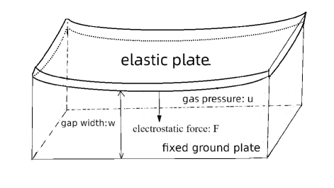
Figure 1: Idealized electrostatically actuated MEMS capacitor.

Our proof of Theorem 1.1 relies on the techniques for quasilinear parabolic equations developed, for example, by Amann, Arendt, Lunardi and Sinestrari [1, 2, 18, 19, 21, 22, 27]. Semigroup methods of this kind have become a powerful tool for MEMS-related models defined by a single equation or by an elliptic-parabolic coupled system, see the recent survey [16]. We here combine such parabolic techniques for the quasilinear Reynolds’ equation (1.1a) with semigroup techniques for the semilinear fourth-order equation (1.1b).

In the recent work [11] the authors showed the wellposedness of a related, simpler model in which (1.1a) is replaced by a linear, elliptic equation for the gas pressure $u$. Physically, the simpler model in [11] replaces the dynamics of $u$ by a quasi-static approximation which can apply in limiting cases; here we consider the more accurate, fuller model to give a good representation of the physical system outlined in Figure 1. Technically, the analysis of both coupled systems relies on a delicate combination of the techniques available for the constituent equations. In the recent work [11] the well-known analysis of linear, elliptic equations allowed us to reduce the simpler model to a perturbed semilinear dispersive equation for the gap width $w$, which is studied using strongly continuous semigroup techniques for such equations. For the realistic model (1.1a)-(1.1d) considered here, similarly complete information is not available for the quasilinear, degenerately parabolic equation (1.1a). Nevertheless, by refining the analysis of (1.1b), we here reduce the coupled system to an abstract quasilinear, degenerately parabolic equation for the gas pressure $u$, for which we are able to show wellposedness. Analytic semigroup techniques allow us to study this quasilinear, degenerately parabolic equation.

The model (1.1) gives the behaviour of a basic electrically actuated MEMS (Micro-Electro-Mechanical Systems) capacitor (see, e.g., [26]). This device contains two conducting plates which are close and parallel to each other when the device is uncharged and at equilibrium. We take, more generally, a fixed potential difference to be applied; this potential difference acts across the plates and the MEMS device forms a capacitor. The two plates lie inside a sealed box also containing a gas, with pressure substantially below atmospheric but not a perfect vacuum. The gas gives a small resistance to the motion of the upper, plate, which is taken to be flexible but pinned around its edges. The other, lower, plate is assumed perfectly rigid and flat. See Figure 1. Breakdown of the device can occur through a pull-in instability, when the two plates touch, the physical phenomenon described by quenching.

Eqn. (1.1a) is a compressible form of the standard Reynolds’ equation for the pressure, $u$, in the gap between the plates, where the local gap width is $w$ (see, for example, [23]), and the gas is assumed to behave ideally and isothermally, so that its density can be taken to be proportional to pressure; this contrasts with the incompressible, liquid-like representation in [11].

The upper electrode of the capacitor moves as a thin elastic plate, so that it behaves according to a dynamic plate equation balancing the inertial term on the left-hand side of (1.1b) with:

• tension terms applied across the plate leading to the usual Laplacian (the first term on the right);

• a biharmonic term modelling linear elasticity (the second term on the right) [14];

• an electrostatic force attracting the upper plate towards the lower (the third term on the right) – strength of this force per unit area is given by the local electric field strength times the surface charge density, the latter itself being proportional to the former, while this, the field strength, is inversely proportional to the gap width $w$;

• net upward gas pressure acting on the plate – pressure in the gap acting up and constant ambient pressure acting down (the final term on the right).

For more details see [25], [26].

The terms in the equations have been scaled to obtain unit coefficients in (1.1a). Without loss of generality, we have taken, for simplicity, various coefficients of terms in (1.1b) also to be one. This does not affect our analysis of the problem.

In another, forthcoming paper, we study the limiting case where the movement of the upper plate is dominated by its tension, so that elastic effects are negligible. This approximation leads to a wave equation for the gap width $w$, instead of the dispersive equation (1.1b).

We review various previous models for electrostatic MEMS devices, some taking the form of a single equation others a coupled system. We also review literature which studies these models, both numerically and analytically, to obtain qualitative behaviour.

As the elastic plate in a MEMS device is fabricated at a micro-scale, the electrostatic force becomes relatively large so that it is the key force causing the bending of the plate when the device operates. The electrostatic force is inversely proportional to the square of the gap width between the two plates(see [8], [25], Sec. 3.4 of [26]), so that the distributed transverse load is the electrostatic force per area is $F_{d}$,

$$F_{d}=-\frac{\beta_{F}}{w^{2}},\quad\text{where}\ \beta_{F}\ \text{is an electrostatic coefficient}.$$ (1.3)

Hence, the static deflection of charged elastic plates in electrostatic actuators can be represented by a nonlinear elliptic equation

$$-\Delta w+\beta_{e}\Delta^{2}w=-\frac{\beta_{F}}{w^{2}}.$$ (1.4)

Lin et al. [17] study the existence, construction, approximation, and behaviour of classical and singular solutions to equation (1.4). Other such problems can be found in references [7], [31].

From Chapter 12 in book [8], there is a value $\beta^{*}\in(0,\infty)$ such that for $0<\beta_{F}<\beta^{*}$ there exists at least one weak solution to (1.4), while no solution exists for $\beta_{F}>\beta^{*}$.

To more fully model the behaviour of the plate, we consider the momentum of the plate as it is deformed, the elastic nature of plate, damping forces, and the electrostatic force between two plates and get an equation of motion

$$\epsilon^{2}\frac{\partial^{2}w}{\partial t^{2}}+\frac{\partial w}{\partial t}-\Delta w+\beta_{e}\Delta^{2}w=-\frac{\beta_{F}}{w^{2}}.$$ (1.5)

Here the gap width $w=w(x,t)$ depends on time $t$ and point $x$ on the surface of movable plate, $\frac{\partial w}{\partial t}$ is a damping term,

$$\epsilon^{2}=\frac{\text{inertial\ coefficient}}{\text{damping\ coefficient}},$$

$\beta_{e}$ accounts for the relative importance of tension and flexural rigidity in the elastic plate, $\beta_{F}$ is proportional to the square of the applied voltage.

Considering the equation defined on a bounded domain of $\mathbb{R}^{n}$, $1\leq n\leq 3$, Guo, [13], finds that when a voltage – represented here mathematically by $\beta_{F}$ – is applied, the elastic plate deflects towards the ground plate, and quenching may occur when $\beta_{F}$ exceeds the critical value $\beta^{*}$ for the time-independent problem (1.4). Guo [13] shows that there exists a $\beta_{F_{1}}\in(0,\ \beta^{*}]$ such that for $0\leq\beta_{F}<\beta_{F_{1}}$, the solution of an initial boundary value problem for (1.5) globally exists. Under some further technical hypotheses, in this case the solution exponentially converges to a regular steady state. For $\beta_{F}>\beta^{*}$, the solution quenches at finite time.

Recent publications only study the compressible version (1.1b) of the standard Reynolds’ equation numerically, and this can be seen in the works [3, 5, 28, 29]. In particular, Bao et al. [4] study the squeeze film damping with small amplitude deflections and linearize the nonlinear Reynolds’ equation (i.e. (1.1b)) around the equilibrium position. The resulting equation is regarded as a form of the heat equation and it is possible to find analytical solutions for this.

See the survey article [16] for a discussion of a wider class of models arising in the description of MEMS. We are not aware of any rigorous results for MEMS models which take into account both the dynamics of the gas and the elastodynamics of the plate.

The plan of the paper is as follows: In Section 2, we introduce notation, the relevant function spaces and some of their basic properties. We also introduce the mild solution and strict solution for the general evolution equation and their existence results, and show some Lipschitz continuity estimates. In Section 3, we use a solution strategy for the system (1.1a), (1.1b) based on decoupling the equations for the gap-width $w$ and the pressure $u$. We first consider the semilinear fourth-order equation (1.1b) for the deflection $w$ with an arbitrarily given pressure $u$ and use semigroup techniques for (1.1b) to show that the local wellposedness of (1.1b). While the regularity theory of dispersive equations has been of much recent interest, we here require detailed properties of the solution operator $u\longmapsto w(u)$ in order to analyse the nonlinear Reynolds’ equation (1.1a) with abstract coefficients involving $w(u)$. For example, we prove appropriate Hölder continuity of the solution operator $u\longmapsto w(u)$ in Section 4. In Section 5, we investigate the local wellposedness of (1.1a) for $u$ with abstract coefficients involving $w(u)$ by using techniques for quasilinear parabolic equations.

1.1 Outline

Note that system (1.1) can be written, as long as $w>0$ (no quenching occurs), as a coupled system in the form

$$\frac{\partial u}{\partial t}=\frac{1}{w}\nabla\cdot\left(w^{3}u\nabla u\right)-\frac{v}{w}u,\quad x\in\Omega,\ t\geq 0;$$ (1.6a)

$$\frac{\partial v}{\partial t}=\Delta w-\Delta^{2}w-\frac{\beta_{F}}{w^{2}}+\beta_{p}(u-1),\quad x\in\Omega,\ t\geq 0;$$ (1.6b)

$$\frac{\partial w}{\partial t}=v,\quad x\in\Omega,\ t\geq 0;$$ (1.6c)

with the initial values $u(x,0)=u_{0}(x)$, $v(x,0)=v_{0}(x)$, $w(x,0)=w_{0}(x)$, $x\in{\Omega}$ and boundary values $u(x,t)=\theta_{1}$, $w(x,t)=\theta_{2}$, $\Delta w(x,t)=0$, $x\in\partial\Omega$, $t\geq 0$, where the initial values are compatible with the boundary conditions, i.e. $u_{0}(x)=\theta_{1}$, $w_{0}(x)=\theta_{2}$ and $\Delta w_{0}(x)=0$ for all $x\in\partial\Omega$, moreover, $u_{0}\in H^{2+\sigma}(\Omega)$ with $\sigma\in(0,1)$, $v_{0}\in H^{2}(\Omega)\cap H_{0}^{1}(\Omega)$ and $w_{0}\in H^{4}(\Omega)$, then look for a unique strict solution $(u,v,w)$ of the coupled system (1.6) for short time. Section 3 shows that there exists a unique solution $(v,w)$ of the sub-system (1.6b), (1.6c) for arbitrarily given but appropriately regular $u$, initial values $v(x,0)=v_{0}(x)$, $w(x,0)=w_{0}(x)$, $x\in{\Omega}$ and boundary values $w(x,t)=\theta_{2}$, $\Delta w(x,t)=0$, $x\in\partial\Omega,\ t\geq 0$, then Section 4 establishes relevant properties of solution operators $u\longmapsto v=v(u)$, $u\longmapsto w=w(u)$ for short time $T$ such as:

Theorem 1.3.

The solution operator

$$W:\ C\left(\left[0,T\right],B_{H^{2}}(u_{0},r)\right)\longrightarrow C\left(\left[0,T\right],B_{L^{2}}(v_{0},r)\times B_{H^{2}}(w_{0},r)\right)$$

$$u\longmapsto W(u)=\left(v,w\right)=\left(v(u),w(u)\right)$$

is Lipschitz continuous with respect to $u$, i.e.

$$\left\|W({u}_{1})-W({u}_{2})\right\|_{C\left([0,T];L^{2}(\Omega)\times H^{2}(\Omega)\right)}\leq L_{W}\|{u}_{1}-{u}_{2}\|_{C\left([0,T];H^{2}(\Omega)\right)},$$ (1.7)

where $r>0$ is sufficiently small, $L_{W}>0$ is a Lipschitz constant,

$$B_{H^{2}}(U,r)=\left\{f\in H^{2}(\Omega):\ f|_{\partial\Omega}=U|_{\partial\Omega},\ \|f-U\|_{H^{2}(\Omega)}\leq r\right\},$$

$$B_{L^{2}}(V,r)=\left\{f\in L^{2}(\Omega):\ \|f-V\|_{L^{2}(\Omega)}\leq r\right\}.$$

Corollary 1.4.

For $u\in C\left([0,T];B_{H^{2}}(u_{0},r)\right)$ and a small radius $r>0$, the Fréchet derivative $W^{\prime}(u)$ of $W(u)$, given by

$${W}{{}^{\prime}}(u):C\left([0,T];H^{2}(\Omega)\cap H_{0}^{1}(\Omega)\right)\longrightarrow C\left([0,T];L^{2}(\Omega)\times\left\{H^{2}(\Omega)\cap H_{0}^{1}(\Omega)\right\}\right),$$

$$q\longmapsto W^{\prime}(u)q=\left(v^{\prime}(u)q,w^{\prime}(u)q\right)$$

is Lipschitz continuous with respect to $u$, i.e. for $\left\|q\right\|_{C\left([0,T];H^{2}(\Omega)\right)}\leq 1$,

$$\left\|{W}^{\prime}(u_{1})q-{W}^{\prime}(u_{2})q\right\|_{C\left([0,T];L^{2}(\Omega)\times H^{2}(\Omega)\right)}\leq L_{F}\left\|{u}_{1}-{u}_{2}\right\|_{C\left([0,T];H^{2}(\Omega)\right)}.$$ (1.8)

Here $L_{F}$ is a Lipschitz constant.

Corollary 1.5.

If $r>0$ is small and $u\in C^{\alpha}\left([0,T];B_{H^{2}}(u_{0},r)\right)$, setting $\tilde{u}_{0}=u_{0}-\theta_{1}$, then there exists a Lipschitz constant $L_{M}>0$, such that

$$\sup_{0\leq t<t+h\leq T}\left\|[{W}^{\prime}(u)q](t+h)-[{W}^{\prime}(u)q](t)\right\|_{L^{2}(\Omega)\times H^{2}(\Omega)}\leq h^{\alpha}L_{M}\left\|q\right\|_{C\left([0,T];H^{2}(\Omega)\right)}$$

$$+ h^{\alpha}TL_{M}\left\|q\right\|_{C^{\alpha}\left([0,T];H^{2}(\Omega)\right)}$$

holds for all $q\in C^{\alpha}\left([0,T];B_{H^{2}}(\tilde{u}_{0},r)\right)$.

Section 5 shows an existence result for the coupled system (1.1). The strategy of proof is to reformulate the system (1.1) as the quasilinear parabolic equation with abstract coefficients involving $v(u)$ and $w(u)$

$$\frac{\partial u}{\partial t}=\frac{1}{w(u)}\nabla\cdot\left([w(u)]^{3}u\nabla u\right)-\frac{v(u)}{w(u)}u,\quad(x,t)\in\Omega\times(0,T),$$ (1.9a)

$$u(x,0)=u_{0}(x),\quad x\in\Omega,\quad u(x,t)=\theta_{1},\quad(x,t)\in\partial\Omega\times[0,T],$$ (1.9b)

and then show the solution of (1.9) exists as long as $\left(v(u),w(u)\right)\in C\left([0,T];B_{L^{2}}(v_{0},r)\times B_{H^{2}}(w_{0},r)\right)$ for small $r>0$ and $T>0$ by using a contraction mapping argument.

We set $\tilde{u}=u-\theta_{1}$, where $\tilde{u}(t):\Omega\longrightarrow\mathds{R}$, $x\longmapsto[\tilde{u}(t)](x)=\tilde{u}(x,t)$, $\forall\ t\in[0,T]$,

$$F(\tilde{u})=\frac{1}{w(\tilde{u}+\theta_{1})}\nabla\cdot\left([w(\tilde{u}+\theta_{1})]^{3}(\tilde{u}+\theta_{1})\nabla\tilde{u}\right)-\frac{v(\tilde{u}+\theta_{1})}{w(\tilde{u}+\theta_{1})}(\tilde{u}+\theta_{1}),$$

and start the argument with the definition of linearization $\mathcal{P}^{*}$ of $F(\tilde{u})$ around $\tilde{u}_{0}$,

$$\mathcal{P}^{*}:\ D\left(\mathcal{P}^{*}\right)\subseteq H^{2}(\Omega)\cap H_{0}^{1}(\Omega)\longrightarrow L^{2}(\Omega),$$

$$\mathcal{P}^{*}\psi=\frac{1}{w_{0}}\nabla\cdot\left\{w_{0}^{3}u_{0}\nabla\psi+\left(w_{0}^{3}\nabla u_{0}\right)\psi\right\}-\frac{v_{0}}{w_{0}}\psi,$$

then we show that the operator $\mathcal{P}^{*}$ generates an analytic semigroup $\left\{e^{t\mathcal{P}^{*}}:\ t\geq 0\right\}$ and rewrite (1.9) in the form of

$$\tilde{u}^{\prime}(t)=\mathcal{P}^{*}\tilde{u}(t)+[F(\tilde{u})](t)-\mathcal{P}^{*}\tilde{u}(t),\quad t\in(0,T),\quad\tilde{u}(0)=\tilde{u}_{0}.$$ (1.10)

In order to prove the existence result for the nonlinear problem (1.10), we shall need the following Hölder result which is deduced from Theorem 1.3, Corollary 1.4 and Corollary 1.5.

Lemma 1.6.

If $\tilde{u},\ q\in C^{\alpha}\left([0,T];B_{H^{2}}\left(\tilde{u}_{0},r\right)\right)$, then there exist postive constants $L_{A}$ and $L_{B}$, such that for all $0\leq t<t+h\leq T$,

$$\left\|\left[F(\tilde{u})\right](t+h)-\left[F(\tilde{u})\right](t)\right\|_{L^{2}(\Omega)}\leq\left\{[\tilde{u}+\theta_{1}]_{C^{\alpha}\left(\left[0,T\right];H^{2}(\Omega)\right)}+L_{U}\right\}L_{A}h^{\alpha},$$ (1.11)

$$\left\|\left[F^{\prime}(\tilde{u})q\right](t+h)-\left[F^{\prime}(\tilde{u})q\right](t)-\mathcal{P}^{*}\left[q(t+h)-q(t)\right]\right\|_{L^{2}(\Omega)}$$

$$\leq h^{\alpha}T^{\alpha}L_{B}\left\|q\right\|_{C^{\alpha}([0,T];H^{2}(\Omega))}+h^{\alpha}T^{\alpha}L_{B}\left\|\tilde{u}+\theta_{1}\right\|_{C^{\alpha}([0,T];H^{2}(\Omega))}\left\|q\right\|_{C^{\alpha}([0,T];H^{2}(\Omega))}$$

$$+ h^{\alpha}L_{B}\left\|q\right\|_{C([0,T];H^{2}(\Omega))}+h^{\alpha}L_{B}\left\|\tilde{u}+\theta_{1}\right\|_{C^{\alpha}([0,T];H^{2}(\Omega))}\left\|q\right\|_{C([0,T];H^{2}(\Omega))}.$$ (1.12)

We are going to show that the existence of a unique strict solution of (1.10) by proving there exists $T_{\max}>0$, such that the nonlinear map $\Gamma$ defined by

$$\Gamma(\tilde{u}(t))=e^{t\mathcal{P}^{*}}\tilde{u}_{0}+\displaystyle\int_{0}^{t}e^{(t-s)\mathcal{P}^{*}}\left\{[F(\tilde{u})](s)-\mathcal{P}^{*}\tilde{u}(s)\right\}ds,\quad t\in[0,T],$$ (1.13)

is a contractive map and has a unique fixed point in $C^{\alpha}\left([0,T];H^{2}(\Omega)\cap H_{0}^{1}(\Omega)\right)$ for $T\in[0,T_{\max})$ and $\alpha\in(0,1)$. To prove the assertion, we define

$$Y=\left\{\tilde{u}\in C^{\alpha}\left([0,T];H^{2}(\Omega)\cap H_{0}^{1}(\Omega)\right):\ \tilde{u}(0)=\tilde{u}_{0},\ \left\|\tilde{u}(\cdot)-\tilde{u}_{0}\right\|_{C^{\alpha}([0,T];H^{2}(\Omega))}\leq r\right\},$$

with small $r>0$, by using the Hölder results in Lemma 1.6, we deduce that, there is $T_{\max}>0$, such that, for $T\in(0,T_{\max})$, small $r>0$ and $\alpha\in(0,1)$, $\Gamma$ is a contractive map which maps $Y$ to itself, i.e. $\tilde{u}_{1}$, $\tilde{u}_{2}\in Y$,

$$\left\|\Gamma\tilde{u}_{1}-\Gamma\tilde{u}_{2}\right\|_{C^{\alpha}\left([0,T];H^{2}(\Omega)\right)}\leq\frac{1}{2}\left\|\tilde{u}_{1}-\tilde{u}_{2}\right\|_{C^{\alpha}\left([0,T];H^{2}(\Omega)\right)},\quad\Gamma(Y)\subseteq Y.$$

By the Banach fixed point theorem, we conclude the existence of a unique fixed point in $Y$ which is a unique strict solution of (1.10) belonging to

$$C^{\alpha}\left([0,T];H^{2}(\Omega)\cap H_{0}^{1}(\Omega)\right)\cap C^{\alpha+1}\left([0,T];L^{2}(\Omega)\right),$$

by the regularity results of the evolution equation of parabolic type from [1, 21, 27].

Combining the existence and regularity results from Section 3 with the existence of a unique strict solution of (1.10), we conclude the proof of Theorem 1.1.

2 Preliminaries

In this section, we first formulate some auxiliary results which will be useful in the proof of the main theorem, with the proofs of Lemma 2.2, Lemma 2.3 and Lemma 2.4 being found in Appendix A. We then state a general existence result for evolution equations and the regularity in time without proof.

2.1 Notations

Recall that $\beta_{F}$, $\beta_{p}$, $\theta_{1}$ and $\theta_{2}$ given positive constants. Let $\Omega$ be an open and bounded subset of $\mathds{R}^{n}$ with smooth boundary $\partial\Omega$, $n=1,\ 2$. Denote by $C=C(\Omega)$ a positive constant which may vary from line to line below but only depends on $\Omega$.

Definition 2.1.

Denote by $X$ a Banach space, with norm $\|\cdot\|_{X}$, $k\in\mathbb{N}$ and $T\in(0,\infty)$. $\mathcal{B}(X)$ denotes the space of bounded linear operators on $X$. In the following, we shall be particularly interested in $X=L^{2}(\Omega)$, $L^{\infty}(\Omega)$, $H^{k}(\Omega)$, etc. The space $\mathcal{B}([0,T];X)$ consists of all measurable, almost everywhere bounded functions $u:[0,T]\longrightarrow X$, $t\longmapsto u(t)$, with norm $\|u\|_{\mathcal{B}([0,T];X)}=\sup_{t\in[0,T]}\|u(t)\|_{X}$. If $X$ is a function space as above, we write $u(t):\Omega\longrightarrow\mathds{R}$ with $x\longmapsto[u(t)](x)=u(x,t)$. The closed subspace of continuous functions is denoted by $C([0,T];X)$, and

$$C^{k}([0,T];X)=\left\{u:[0,T]\rightarrow X:\tfrac{d^{j}u}{dt^{j}}\in C([0,T];X),j\in[0,k]\right\},\|u\|_{C^{k}([0,T];X)}=\sup_{t\in[0,T]}\sum_{j=0}^{k}\left\|\tfrac{d^{j}u(t)}{dt^{j}}\right\|_{X}.$$

The definition extends to non-integer order $k+\alpha$, $\alpha\in(0,1)$, by setting

$$C^{\alpha}([0,T];X)=\left\{u:[0,T]\rightarrow X:[u]_{C^{\alpha}([0,T];X)}=\sup_{0\leq t<t+h\leq T}\tfrac{\|u(t+h)-u(t)\|_{X}}{|h|^{\alpha}}<\infty\right\},$$

$$\|u\|_{C^{\alpha}([0,T];X)}=\|u\|_{C([0,T];X)}+[u]_{C^{\alpha}([0,T];X)}.$$

$$C^{\alpha+k}([0,T];X)=\left\{u\in C^{k}([0,T];X):\quad\tfrac{d^{k}u}{dt^{k}}\in C^{\alpha}([0,T];X)\right\},$$

$$\|u\|_{C^{\alpha+k}([0,T];X)}=\|u\|_{C^{k}([0,T];X)}+\left[\tfrac{d^{k}u}{dt^{k}}\right]_{C^{\alpha}([0,T];X)}.$$

Note that $C\left([0,T];B_{L^{2}}\left(V,r\right)\right)=\Big{\{}v\in C\left([0,T];L^{2}\left(\Omega\right)\right):\displaystyle\sup_{t\in[0,T]}\left\|v(t)-V\right\|_{H^{2}(\Omega)}\leq r\Big{\}}$, $V\in L^{2}(\Omega)$, $C\left([0,T];B_{H^{2}}\left(U,r\right)\right)=\Big{\{}u\in C\left([0,T];H^{2}\left(\Omega\right)\right):\ u|_{\partial\Omega}=U|_{\partial\Omega},\ \displaystyle\sup_{t\in[0,T]}\left\|u(t)-U\right\|_{H^{2}(\Omega)}\leq r\Big{\}}$, $C^{\alpha}\left([0,T];B_{H^{2}}\left(U,r\right)\right)=\Big{\{}u\in C^{\alpha}\left([0,T];H^{2}\left(\Omega\right)\right):\ u|_{\partial\Omega}=U|_{\partial\Omega},\ \displaystyle\sup_{t\in[0,T]}\left\|u(t)-U\right\|_{H^{2}(\Omega)}\leq r\Big{\}}$
with $U\in H^{2}(\Omega)$.

If $\mathcal{P}:D(\mathcal{P})\subset X\to X$ is an unbounded linear operator which generates an analytic semigroup $e^{\mathcal{P}t}$, we define intermediate space $D_{\mathcal{P}}(\alpha,\infty)$ as follows:

$$D_{\mathcal{P}}(\alpha,\infty)=\left\{v\in X:\ \|v\|_{\alpha}=\sup_{t>0}\|t^{1-\alpha}\mathcal{P}e^{\mathcal{P}t}v\|_{X}<\infty\right\}.$$

It is a Banach space with respect to the norm $\|v\|_{D_{\mathcal{P}}(\alpha,\infty)}=\|v\|_{X}+\|v\|_{\alpha}$. Its closed subspace $D_{\mathcal{P}}(\alpha)=\left\{v\in X:\ \lim_{t\rightarrow 0}t^{1-\alpha}\mathcal{P}e^{\mathcal{P}t}v=0\right\}$ inherits the norm of $D_{\mathcal{P}}(\alpha,\infty)$.

Our main results on the wellposedness of the semilinear dispersive equation (1.1b) will be shown by constructing a Picard iteration in the complete metric space $\mathcal{Z}(T)$, given by

$$\mathcal{Z}(T): =\bigg{\{}(\tilde{v},\tilde{w})\in C\left([0,T];L^{2}(\Omega)\times H^{2}(\Omega)\right):\ \left(\tilde{v}(0),\tilde{w}(0)\right)=\left(\tilde{v}_{0},\tilde{w}_{0}\right),\quad\tilde{w}|_{\partial\Omega}=\tilde{w}_{0}|_{\partial\Omega},$$

$$\sup_{t\in[0,T]}\|(\tilde{v}(t)-\tilde{v}_{0},\tilde{w}(t)-\tilde{w}_{0})\|_{L^{2}(\Omega)\times H^{2}(\Omega)}\leq r\bigg{\}},\quad\text{where}\quad\tilde{v}_{0}=v_{0},\quad\tilde{w}_{0}=w_{0}-\theta_{2}.$$ (2.1)

2.2 Useful Estimates

The estimates in this subsection are proven in Appendix A.

Lemma 2.2.

There exists a constant $C=C(\Omega)>0$, such that for all

$$r\in\left(0,\ \frac{\kappa}{2C}\right),$$ (2.2)

$w\in C\left([0,T];B_{H^{2}}\left(w_{0},r\right)\right)$ has the lower bound such as

$$w(t)\geq\frac{\kappa}{2},\quad\forall\ t\in[0,T].$$ (2.3)

Moreover, for all $w_{1}$, $w_{2}\in C\left([0,T];B_{H^{2}}(w_{0},r)\right)$, there exist positive constants $C_{k}$, $k=1,\ 2,\ 3$, depending on $\Omega$, $\kappa$ and $\left\|w_{0}\right\|_{H^{2}(\Omega)}$, such that

$$\sup_{t\in[0,T]}\left\|\frac{1}{[w_{1}(t)]^{k}}\right\|_{H^{2}(\Omega)}\leq{C_{1}^{k}},\quad k=1,\ 2,\ 3,$$ (2.4)

$$\sup_{t\in[0,T]}\left\|\frac{1}{[w_{1}(t)]^{k}}-\frac{1}{[w_{2}(t)]^{k}}\right\|_{H^{2}(\Omega)}\leq C_{k}\sup_{t\in[0,T]}\left\|w_{1}(t)-w_{2}(t)\right\|_{H^{2}(\Omega)},\ k=2,\ 3.$$ (2.5)

Lemma 2.3.

The nonlinear operator $G$, defined by

$$G:\ C\left([0,T];B_{H^{2}}\left(\tilde{w}_{0},r\right)\right)\longrightarrow C([0,T];H^{2}(\Omega)),\quad\tilde{w}\longmapsto G(\tilde{w})$$

$$[G(\tilde{w})](t)=G(\tilde{w}(t))=-\frac{\beta_{F}}{[\tilde{w}(t)+\theta_{2}]^{2}}+\beta_{p}(\theta_{1}-1),$$

has the following properties:

$$\sup_{0\leq t<t+h\leq T}\left\|[G(\tilde{w})](t+h)-[G(\tilde{w})](t)\right\|_{H^{2}(\Omega)}\leq L_{G}\sup_{0\leq t<t+h\leq T}\left\|\tilde{w}(t+h)-\tilde{w}(t)\right\|_{H^{2}(\Omega)},$$ (2.6)

$$\sup_{t\in[0,T]}\left\|[G(\tilde{w}_{1})](t)-[G(\tilde{w}_{2})](t)\right\|_{H^{2}(\Omega)}\leq L_{G}\sup_{t\in[0,T]}\left\|\tilde{w}_{1}(t)-\tilde{w}_{2}(t)\right\|_{H^{2}(\Omega)},$$ (2.7)

$$\sup_{t\in[0,T]}\left\|[G(\tilde{w}_{1})](t)-G(\tilde{w}_{0})\right\|_{H^{2}(\Omega)}\leq L_{G}r.$$ (2.8)

Here $L_{G}=L_{G}\left(\Omega,\ \kappa,\ \|w_{0}\|_{H^{2}(\Omega)},\ \beta_{F}\right)$ is a constant.
Furthermore, the Fréchet derivative $G^{\prime}(\tilde{w})$ of $G(\tilde{w})$ on $\tilde{w}\in C\left([0,T];B_{H^{2}}\left(\tilde{w}_{0},r\right)\right)$, defined by

$$G^{\prime}\left(\tilde{w}\right):\ C\left([0,T];H^{2}(\Omega)\cap H_{0}^{1}(\Omega)\right)\longrightarrow C\left([0,T];H^{2}(\Omega)\cap H^{1}_{0}(\Omega)\right),\quad q\longmapsto G^{\prime}\left(\tilde{w}\right)q,$$

$$\left[G^{\prime}\left(\tilde{w}\right)q\right](t)=\left[G^{\prime}\left(\tilde{w}(t)\right)\right]q(t)=\frac{2\beta_{F}}{\left(\tilde{w}(t)+\theta_{2}\right)^{3}}q(t),$$

satisfies

$$\sup_{t\in[0,T]}\left\|\left[G^{\prime}\left(\tilde{w}\right)q\right](t)\right\|_{H^{2}(\Omega)}\leq L_{G}\sup_{t\in[0,T]}\left\|q(t)\right\|_{H^{2}(\Omega)},$$ (2.9)

and $G^{\prime}(\tilde{w}(t)):\left\{H^{2}(\Omega)\cap H_{0}^{1}(\Omega)\right\}\longrightarrow\left\{H^{2}(\Omega)\cap H_{0}^{1}(\Omega)\right\}$ satisfies

$$\lim_{h\rightarrow 0}\sup_{\begin{smallmatrix}0\leq t\leq t+h\leq T\\ 0\leq\tau\leq 1\end{smallmatrix}}\left\|G^{\prime}\left(\tilde{w}(t)+\tau\left[\tilde{w}(t+h)-\tilde{w}(t)\right]\right)-G^{\prime}\left(\tilde{w}(t)\right)\right\|_{\mathcal{B}\left(H^{2}(\Omega)\right)}=0.$$ (2.10)

Lemma 2.4.

Assume the operators $u\longmapsto v(u)$ and $u\longmapsto w(u)$, respectively given by

$$u\longmapsto v(u):\quad C\left([0,T];B_{H^{2}}\left(u_{0},r\right)\right)\longrightarrow C\left([0,T];B_{L^{2}}\left(v_{0},r\right)\right),$$

$$u\longmapsto w(u):\quad C\left([0,T];B_{H^{2}}\left(u_{0},r\right)\right)\longrightarrow C\left([0,T];B_{H^{2}}\left(v_{0},r\right)\right),$$

satisfy, for all $u_{1},\ u_{2}\in C\left([0,T];B_{H^{2}}\left(u_{0},r\right)\right)$,

$$\sup_{t\in[0,T]}\|[v(u_{1})](t)-[v(u_{2})](t)\|_{L^{2}(\Omega)}\leq L_{W}\sup_{t\in[0,T]}\|{u}_{1}(t)-{u}_{2}(t)\|_{H^{2}(\Omega)},$$

$$\sup_{t\in[0,T]}\|[w(u_{1})](t)-[w(u_{2})](t)\|_{H^{2}(\Omega)}\leq L_{W}\sup_{t\in[0,T]}\|{u}_{1}(t)-{u}_{2}(t)\|_{H^{2}(\Omega)}.$$

Then $f(u)$, defined by

$$u\longmapsto f(u):C\left([0,T];B_{H^{2}}\left(u_{0},r\right)\right)\longrightarrow C([0,T];L^{2}(\Omega)),\quad f(u)=\frac{1}{w(u)}\nabla\cdot\left([w(u)]^{3}u\nabla u\right)-\frac{v(u)}{w(u)}u,$$

is Lipschitz continuous in $u$,

$$\sup_{t\in[0,T]}\|[f(u_{1})](t)-[f(u_{2})](t)\|_{L^{2}(\Omega)}\leq L_{e}\sup_{t\in[0,T]}\|{u}_{1}(t)-{u}_{2}(t)\|_{H^{2}(\Omega)}.$$ (2.11)

Here $L_{W}$ and $L_{e}$ are Lipschitz constants, and $L_{e}$ depends on $L_{W}$, $\Omega$, $\kappa$, $\left\|u_{0}\right\|_{H^{2}(\Omega)}$, $\left\|v_{0}\right\|_{L^{2}(\Omega)}$, $\left\|w_{0}\right\|_{H^{2}(\Omega)}$.

2.3 Properties of Evolution Equations

We recall standard notions and results for abstract evolution equations.

Definition 2.5.

Let $\mathfrak{X}$ be a Banach space, $\mathcal{A}:D(\mathcal{A})\subset\mathfrak{X}\to\mathfrak{X}$ a linear, unbounded operator which generates a strongly continuous semigroup ($C_{0}$-semigroup) $\{T(t):t\geq 0\}$. Further, let $T\in(0,\infty)$, $\mathcal{G}\in C([0,T];\mathfrak{X})$ and $\Phi_{0}\in\mathfrak{X}$. A function $\Phi$ is called a mild solution of the inhomogeneous evolution equation

$$\Phi^{\prime}(t)=\mathcal{A}\Phi(t)+\mathcal{G}(t),\quad t\in[0,T],\quad\Phi(0)=\Phi_{0},$$ (2.12)

if $\Phi\in C([0,T];\mathfrak{X})$ is given by the integral formulation

$$\Phi(t)=T(t)\Phi_{0}+\int_{0}^{t}T(t-s)\mathcal{G}(s)ds,\quad t\in[0,T].$$ (2.13)

A function $\Phi$ is said to be a strict solution of (2.12), if $\Phi\in C([0,T];D(\mathcal{A}))\cap C^{1}([0,T];\mathfrak{X})$ is given by the integral formulation (2.13) and satisfies (2.12).

Lemma 2.6.

Let the linear operator $\mathcal{A}$ defined on a Banach space $\mathfrak{X}$ generate the $C_{0}$-semigroup $\{T(t):t\geq 0\}$, $T\in(0,\infty)$, and $\Phi_{0}\in D(\mathcal{A})$. If $\mathcal{G}\in C([0,T];\mathfrak{X})$ and $\Phi$ is a solution of the inhomogeneous evolution equation (2.12), then $\Phi$ is given by the integral formulation (2.13).

Assume either that $\mathcal{G}\in C([0,T];D(\mathcal{A}))$ or that $\mathcal{G}\in C^{1}([0,T];\mathfrak{X})$. Then the mild solution $\Phi$ defined by (2.13) uniquely solves the inhomogeneous evolution equation (2.12) on $[0,T]$, and

$$\Phi\in C([0,T];D(\mathcal{A}))\cap C^{1}([0,T];\mathfrak{X}).$$

The proof of Lemma 2.6 is given in [15], Theorem 6.9.

Lemma 2.7.

Let $\mathfrak{X}$ be a Banach space and $\Phi\in C([0,T];\mathfrak{X})$ be differentiable from the right with right derivative $\Psi\in C\left([0,T];\mathfrak{X}\right)$. Then $\Phi\in C^{1}\left([0,T];\mathfrak{X}\right)$ and $\Phi^{\prime}=\Psi$.

The proof of Lemma 2.7 is given in [15], Lemma 8.9.

3 Wellposedness of the Dispersive Equation

Refined Analysis of the Dispersive Equation

Denote by $H_{*}^{2}(\Omega):=H^{2}(\Omega)\cap H_{0}^{1}(\Omega)$, $H_{*}^{4}(\Omega):=\left\{\chi\in H^{4}(\Omega):\ \chi|_{\partial\Omega}=\Delta\chi|_{\partial\Omega}=0\right\}$. Take $T\in(0,\infty)$ to be specified below. We first introduce a state $\mathbf{a}=\left(a_{1},\ a_{2}\right)$ and a state space

$$\mathfrak{X}=L^{2}(\Omega)\times H_{*}^{2}(\Omega)$$ (3.1)

with its norm $\|\cdot\|_{\mathfrak{X}}=\left\|\cdot\right\|_{L^{2}(\Omega)\times H^{2}(\Omega)}$ and its scalar product

$$\langle\mathbf{a},\mathbf{b}\rangle_{\mathfrak{X}}=\displaystyle\int_{\Omega}a_{1}\cdot{b_{1}}+\nabla a_{2}\cdot\nabla{b_{2}}+\Delta a_{2}\cdot\Delta{b_{2}}\ {d}x,\quad\mathbf{a}=\left(a_{1},a_{2}\right)\in\mathfrak{X},\ \mathbf{b}=\left(b_{1},b_{2}\right)\in\mathfrak{X}.$$

We then define a linear operator $\mathbb{A}$ by

$$D(\mathbb{A}):= \left\{\phi\in H_{*}^{2}(\Omega):\exists\ f\in L^{2}(\Omega),\ \forall\ \psi\in H_{*}^{2}(\Omega),\ \text{s.t.}\ \int_{\Omega}\nabla\phi\cdot\nabla{\psi}+\Delta\phi\cdot\Delta{\psi}dx=\int_{\Omega}f\cdot{\psi}dx\right\},$$

$$\mathbb{A}\phi:= -f,\ \text{where}\ f\ \text{is given by}\ D(\mathbb{A}),\quad\left\|\phi\right\|_{D(\mathbb{A})}:=\left\|\phi\right\|_{L^{2}(\Omega)}+\left\|\mathbb{A}\phi\right\|_{L^{2}(\Omega)}.$$ (3.2)

It is easy to see that $\Delta\phi|_{\partial\Omega}=0$ for all $\phi\in D(\mathbb{A})$, and from elliptic regularity theory, it follows that

$$D(\mathbb{A})=\left\{\chi\in H^{4}(\Omega):\ \chi|_{\partial\Omega}=\Delta\chi|_{\partial\Omega}=0\right\}=H_{*}^{4}(\Omega),\quad\left\|\chi\right\|_{D(\mathbb{A})}\simeq\|\chi\|_{H^{4}(\Omega)}.$$ (3.3)

We further define the linear operator $\mathcal{A}$ with its domain $D(\mathcal{A})$ and its graph norm $\|\cdot\|_{D(\mathcal{A})}$ by

$$\mathcal{A}=\begin{pmatrix}0\ &\mathbb{A}\\ 1\ &0\end{pmatrix},\quad D(\mathcal{A})=H_{*}^{2}(\Omega)\times H_{*}^{4}(\Omega),$$ (3.4a)

$$\|\mathbf{a}\|_{D(\mathcal{A})}:=\|\mathbf{a}\|_{\mathfrak{X}}+\|\mathcal{A}\mathbf{a}\|_{\mathfrak{X}}\simeq\|a_{1}\|_{H^{2}(\Omega)}+\|a_{2}\|_{H^{4}(\Omega)},\quad\mathbf{a}=\left(a_{1},a_{2}\right)\in D(\mathcal{A}).$$ (3.4b)

We now consider the initial-boundary problem of semilinear fourth-order equation (1.1b) on the unknown function $w$ with an arbitrarily given but fixed $u\in C\left([0,T];B_{H^{2}}\left(u_{0},r\right)\right)$, initial values

$$w(x,0)=w_{0}(x),\quad\frac{\partial w}{\partial t}(x,0)=v_{0}(x),\quad x\in\Omega,$$ (3.5)

and pinned boundary conditions

$$w(x,t)=\theta_{2},\quad\Delta w(x,t)=0,\quad(x,t)\in\partial\Omega\times[0,T].$$ (3.6)

We set $\tilde{w}(x,t)=w(x,t)-\theta_{2}$, where $\tilde{w}(t):\Omega\longrightarrow\mathds{R}$, $x\longmapsto[\tilde{w}(t)](x)=\tilde{w}(x,t)$. Note that the operator $\mathbb{A}$, defined in (3.2), is a realisation of the differential expression $\Delta-\Delta^{2}$ from equation (1.1b) for the pinned boundary conditions $\tilde{w}(x,t)=0$, $\Delta\tilde{w}(x,t)=0$, $x\in\partial\Omega$, $t\in[0,T]$. Using the definition of $\mathbb{A}$, we rewrite (1.1b) with (3.5) and (3.6) as the equation (3.7) for the unknown function $\tilde{w}$:

$$\tilde{w}^{{}^{\prime\prime}}(t)=\mathbb{A}\tilde{w}(t)-\frac{\beta_{F}}{(\tilde{w}(t)+\theta_{2})^{2}}+\beta_{p}(\tilde{u}(t)+\theta_{1}-1),\ t\in[0,T],\ \tilde{w}(0)=\tilde{w}_{0},\ \tilde{w}^{\prime}(0)=\tilde{v}_{0},$$ (3.7)

where $\tilde{w}^{\prime}$ and $\tilde{w}^{{}^{\prime\prime}}$ respectively denote the first and second derivative of the unknown function $\tilde{w}$ with respect to $t\in[0,T]$, $\tilde{u}=u-\theta_{1}$ is given in $C\left([0,T];B_{H^{2}}\left(\tilde{u}_{0},r\right)\right)$ with $\tilde{u}_{0}=u_{0}-\theta_{1}$, $\tilde{v}_{0}=v_{0}$, $\tilde{w}_{0}=w_{0}-\theta_{1}$ and $\tilde{u}_{0}(x)=\tilde{w}_{0}(x)=0$ for all $x\in\partial\Omega$. We further introduce a new time-dependent state $\Phi(t)=\left(\varphi_{1}(t),\ \varphi_{2}(t)\right)$, $t\in[0,T]$, and set

$$[G(\varphi_{2})](t)=-\frac{\beta_{F}}{(\varphi_{2}(t)+\theta_{2})^{2}}+\beta_{p}(\theta_{1}-1),\quad\mathcal{G}=\left[\mathcal{G}\left(\Phi\right)\right](t)=\left(\left[G\left({\varphi}_{2}\right)\right](t)+\beta_{p}\tilde{u}(t),0\right),$$ (3.8)

$$\Phi_{0}=\left(\tilde{v}_{0},\tilde{w}_{0}\right)\in D(\mathcal{A}).$$ (3.9)

We are going to prove that the semilinear fourth-order equation (3.7) has a unique strict solution by showing Lemma 3.1, Lemma 3.2, Theorem 3.3, Corollary 3.4, Corollary 3.5 and Theorem 3.6 in Appendix B. This would conclude the wellposedness of the dispersive equation (1.1b).

Lemma 3.1.

Let given $\tilde{u}\in C\left([0,T];B_{H^{2}}\left(\tilde{u}_{0},r\right)\right)\cap C^{1}\left([0,T];L^{2}(\Omega)\right)$, $\mathcal{A}$ and $\mathcal{G}$ be defined by (3.4) and (3.8) respectively. The semilinear fourth-order equation (3.7) has a unique solution

$$\tilde{w}\in C^{2}\left([0,T];L^{2}(\Omega)\right)\cap C^{1}\left([0,T];H_{*}^{2}(\Omega)\right)\cap C\left([0,T];H_{*}^{4}(\Omega)\right)$$

if and only if the semilinear evolution equation

$$\Phi^{\prime}(t)=\mathcal{A}\Phi(t)+\left[\mathcal{G}\left(\Phi\right)\right](t),\ t\in[0,T],\ \Phi(0)=\Phi_{0},$$ (3.10)

has a unique solution

$$\Phi\in C([0,T];D(\mathcal{A}))\cap C^{1}([0,T];\mathfrak{X}).$$

If this is the case, we have $\Phi=\left(\tilde{w}^{\prime},\tilde{w}\right)$.

Lemma 3.2.

Let $\Omega$ be an open and bounded subset of $\mathds{R}^{n}$ with smooth boundary $\partial\Omega$, $n=1,\ 2$. Then the linear operator $\mathcal{A}$, defined by (3.4), generates a strongly continuous semigroup ($C_{0}$-semigroup) $\left\{T(t)\in\mathcal{B}\left(\mathfrak{X}\right):t\in[0,\infty)\right\}$.

Theorem 3.3.

For $r\in\left(0,\frac{\kappa}{2C}\right)$, there exist $T_{0}>0$, such that for $T\in(0,T_{0})$ and given function $\tilde{u}\in C\left([0,T];B_{H^{2}}\left(\tilde{u}_{0},r\right)\right)$, the semilinear evolution equation (3.11) on $(\tilde{v},\tilde{w})$,

$$\begin{pmatrix}\tilde{v}^{\prime}(t)\\ \tilde{w}^{\prime}(t)\end{pmatrix}=\mathcal{A}\begin{pmatrix}\tilde{v}(t)\\ \tilde{w}(t)\end{pmatrix}+\begin{pmatrix}[G(\tilde{w})](t)+\beta_{p}\tilde{u}(t),\\ 0\end{pmatrix},\ t\in[0,T],\ \begin{pmatrix}\tilde{v}(0)\\ \tilde{w}(0)\end{pmatrix}=\begin{pmatrix}\tilde{v}_{0}\\ \tilde{w}_{0}\end{pmatrix},$$ (3.11)

has a unique mild solution $\left(\tilde{v},\tilde{w}\right)\in C\left([0,T];L^{2}(\Omega)\times H_{*}^{2}(\Omega)\right)$ defined by

$$\begin{pmatrix}\tilde{v}(t)\\ \tilde{w}(t)\end{pmatrix}=T(t)\begin{pmatrix}\tilde{v}_{0}\\ \tilde{w}_{0}\end{pmatrix}+\displaystyle\int_{0}^{t}\left\{T(t-s)\begin{pmatrix}[G(\tilde{w})](s)+\beta_{p}\tilde{u}(s)\\ 0\end{pmatrix}\right\}ds.$$ (3.12)

Corollary 3.4.

Let $T\in(0,T_{0})$ and $\tilde{u}\in C\left([0,T];B_{H^{2}}\left(\tilde{u}_{0},r\right)\right)\cap C^{1}\left([0,T];L^{2}(\Omega)\right)$. Then the mild solution of the semilinear evolution equation (3.11), $\left(\tilde{v},\tilde{w}\right):[0,T]\longrightarrow L^{2}(\Omega)\times H_{*}^{2}(\Omega)$, defined by the integral form (3.12), is locally Lipschitz continuous with respect to $t\in[0,T]$, i.e. $\forall\ h\in(0,T]$,

$$\sup_{0\leq t<t+h\leq T}\left\|\begin{pmatrix}\tilde{v}(t+h)-\tilde{v}(t)\\ \tilde{w}(t+h)-\tilde{w}(t)\end{pmatrix}\right\|_{L^{2}(\Omega)\times H^{2}(\Omega)}\leq L_{V}h.$$ (3.13)

Here $L_{V}$ is a Lipschitz constant depending on $\beta_{F}$, $\beta_{p}$, $T_{0}$, $\kappa$, $\Omega$, $\left\|\tilde{u}_{0}\right\|_{H^{2}(\Omega)}$, $\|\tilde{w}_{0}\|_{H^{2}(\Omega)}$,
$\left\|\left(\tilde{v}_{0},\tilde{w}_{0}\right)\right\|_{D(\mathcal{A})}$, $M_{0}=\displaystyle\sup_{t\in[0,\infty)}\left\|T(t)\right\|_{\mathcal{B}(L^{2}(\Omega)\times H^{2}(\Omega))}$, $\left\|\tilde{u}\right\|_{C^{1}\left([0,T_{0});L^{2}(\Omega)\right)}$.

Corollary 3.5.

If $\alpha\in(0,1)$, $T\in(0,T_{0})$ and given $\tilde{u}\in C^{\alpha}\left([0,T];B_{H^{2}}(\tilde{u}_{0},r)\right)$, then the mild solution of the semilinear evolution equation (3.11), $\left(\tilde{v},\tilde{w}\right):[0,T]\longrightarrow L^{2}(\Omega)\times H_{*}^{2}(\Omega)$, defined by the integral formulation (3.12), is locally Hölder continuous with exponent $\alpha$ with respect to $t\in[0,T]$, i.e.

$$\sup_{0\leq t<t+h\leq T}\left\|\begin{pmatrix}\tilde{v}(t+h)-\tilde{v}(t)\\ \tilde{w}(t+h)-\tilde{w}(t)\end{pmatrix}\right\|_{L^{2}(\Omega)\times H^{2}(\Omega)}\leq L_{U}h^{\alpha},\quad\forall\ h\in(0,T].$$ (3.14)

Here $L_{U}$ is a Lipschitz constant depending on $\alpha$, $T_{0}$, $\kappa$, $\Omega$, $\beta_{p}$, $\beta_{F}$, $\left\|\tilde{u}_{0}\right\|_{H^{2}(\Omega)}$, $\left\|\tilde{w}_{0}\right\|_{H^{2}(\Omega)}$,
$\left\|\left(\tilde{v}_{0},\tilde{w}_{0}\right)\right\|_{D(\mathcal{A})}$ and $M_{0}=\displaystyle\sup_{t\in[0,\infty)}\left\|T(t)\right\|_{\mathcal{B}\left(L^{2}(\Omega)\times H^{2}(\Omega)\right)}$.

Theorem 3.6.

For given $\tilde{u}\in C\left([0,T];B_{H^{2}}\left(\tilde{u}_{0},r\right)\right)\cap C^{1}\left([0,T];L^{2}(\Omega)\right)$ and $T\in(0,T_{0})$, the mild solution $\left(\tilde{v},\tilde{w}\right)$ of the semilinear evolution equation (3.11), defined by the integral form (3.12), is the strict solution of equation (3.11) and

$$\left(\tilde{v},\tilde{w}\right)\in C^{1}\left([0,T];L^{2}(\Omega)\times H_{*}^{2}(\Omega)\right)\cap C\left([0,T];H_{*}^{2}(\Omega)\times H_{*}^{4}(\Omega)\right).$$

4 Solution Operators

Theorem 4.1.

Let $T_{0}$ be given by Theorem 3.3 and $T\in(0,T_{0})$. Then a solution operator, given by

$$W_{1}:\ C\left([0,T];B_{H^{2}}\left(\tilde{u}_{0},r\right)\right)\longrightarrow\mathcal{Z}(T),\quad\tilde{u}\longmapsto W_{1}(\tilde{u})=\left(\tilde{v},\tilde{w}\right)=\left(\tilde{v}(\tilde{u}),\tilde{w}(\tilde{u})\right),\quad r\in\left(0,\frac{\kappa}{2C}\right)$$

with

$$[W_{1}(\tilde{u})](t)=\displaystyle T(t)\begin{pmatrix}\tilde{v}_{0}\\ \tilde{w}_{0}\end{pmatrix}+\int_{0}^{t}\left\{T(t-s)\begin{pmatrix}[G(\tilde{w})](s)+\beta_{p}\tilde{u}(s)\\ 0\end{pmatrix}\right\}ds,\quad t\in[0,T].$$

has Lipschitz continuity, i.e.

$$\sup_{t\in[0,T]}\left\|[W_{1}(\tilde{u}_{1})](t)-[W_{1}(\tilde{u}_{2})](t)\right\|_{L^{2}(\Omega)\times H^{2}(\Omega)}\leq L_{W}\sup_{t\in[0,T]}\|\tilde{u}_{1}(t)-\tilde{u}_{2}(t)\|_{H^{2}(\Omega)}.$$ (4.1)

Here $L_{W}$ is a Lipschitz constant depending on $T_{0}$, $M_{0}=\displaystyle\sup_{t\in[0,\infty)}\left\|T(t)\right\|_{\mathcal{B}\left(L^{2}(\Omega)\times H^{2}(\Omega)\right)}$, $\kappa$, $\|w_{0}\|_{H^{2}(\Omega)}$, $\Omega$, and the coefficients $\beta_{p}$ and $\beta_{F}$. Furthermore, let

$$W_{2}:C\left([0,T];B_{H^{2}}\left(\tilde{u}_{0},r\right)\right)\longrightarrow C([0,T];L^{2}(\Omega)),\quad\tilde{u}\longmapsto\frac{\tilde{v}}{\tilde{w}+\theta_{2}}.$$

Then $W_{2}(\tilde{u})$ also depends Lipschitz-continuously on $\tilde{u}\in C\left([0,T];B_{H^{2}}\left(\tilde{u}_{0},r\right)\right)$, i.e.

$$\sup_{t\in[0,T]}\left\|[W_{2}(\tilde{u}_{1})](t)-[W_{2}(\tilde{u}_{2})](t)\right\|_{L^{2}(\Omega)}\leq L_{W_{2}}\displaystyle\sup_{t\in[0,T]}\|\tilde{u}_{1}(t)-\tilde{u}_{2}(t)\|_{H^{2}(\Omega)},$$ (4.2)

where $L_{W_{2}}$ is a Lipschitz constant depending on above $L_{W}$ and $\left\|\tilde{v}_{0}\right\|_{L^{2}(\Omega)}$.

Proof.

For $T\in(0,T_{0})$, $\tilde{u}_{1}$, $\tilde{u}_{2}\in C\left([0,T];B_{H^{2}}\left(\tilde{u}_{0},r\right)\right)$, $W_{1}(\tilde{u}_{1})=\left(\tilde{v}_{1},\tilde{w}_{1}\right)$, $W_{1}(\tilde{u}_{2})=\left(\tilde{v}_{2},\tilde{w}_{2}\right)$ belong to $\mathcal{Z}(T)$, then it folows that

$$[G(\tilde{w}_{1})](t)-[G(\tilde{w}_{2})](t)+\beta_{p}\tilde{u}_{1}(t)-\beta_{p}\tilde{u}_{2}(t)\in H^{2}(\Omega),\quad\forall\ t\in[0,T],$$

and one can have the following estimates

$$\|[W_{1}(\tilde{u}_{1})](t)-[W_{1}(\tilde{u}_{2})](t)\|_{L^{2}(\Omega)\times H^{2}(\Omega)}$$

$$= \left\|\int_{0}^{t}\displaystyle T(t-s)\begin{pmatrix}[G(\tilde{u}_{1},\tilde{w}_{1})](s)-[G(\tilde{u}_{2},\tilde{w}_{2})](s)\\ 0\end{pmatrix}ds\right\|_{L^{2}(\Omega)\times H^{2}(\Omega)}$$

$$\leq M_{0}\int_{0}^{t}\left\|[G(\tilde{w}_{1})](s)-[G(\tilde{w}_{2})](s)+\beta_{p}\left[\tilde{u}_{1}(s)-\tilde{u}_{2}(s)\right]\right\|_{L^{2}(\Omega)}ds$$

$$\leq M_{0}\int_{0}^{t}\left\|[G(\tilde{w}_{1})](s)-[G(\tilde{w}_{2})](s)+\beta_{p}\left[\tilde{u}_{1}(s)-\tilde{u}_{2}(s)\right]\right\|_{H^{2}(\Omega)}ds,$$ (4.3)

where $M_{0}$ is a operator norm of $\left\{T(t)\in\mathcal{B}\left(L^{2}(\Omega)\times H_{*}^{2}(\Omega)\right):\ t\in[0,\infty)\right\}$. We notice that,

$$\|\tilde{w}_{1}(t)-\tilde{w}_{2}(t)\|_{H^{2}(\Omega)} \leq\left\|\begin{pmatrix}\tilde{v}_{1}(t)-\tilde{v}_{2}(t)\\ \tilde{w}_{1}(t)-\tilde{w}_{2}(t)\end{pmatrix}\right\|_{L^{2}(\Omega)\times H^{2}(\Omega)}$$

$$=\|[W_{1}(\tilde{u}_{1})](t)-[W_{1}(\tilde{u}_{2})](t)\|_{L^{2}(\Omega)\times H^{2}(\Omega)},\quad\forall\ t\in[0,T].$$ (4.4)

Hence combining (4.4) with the Lipschitz continuity estimate (2.7) of $G$ from Lemma 2.3 gives

$$\left\|[G(\tilde{w}_{1})](s)-[G(\tilde{w}_{2})](s)+\beta_{p}\left[\tilde{u}_{1}(s)-\tilde{u}_{2}(s)\right]\right\|_{H^{2}(\Omega)}$$

$$\leq L_{G}\|[W_{1}(\tilde{u}_{1})](s)-[W_{1}(\tilde{u}_{2})](s)\|_{L^{2}(\Omega)\times H^{2}(\Omega)}+\beta_{p}\left\|\tilde{u}_{1}(s)-\tilde{u}_{2}(s)\right\|_{H^{2}(\Omega)},\ \forall\ 0\leq s\leq t\leq T.$$

Hence

$$\|[W_{1}(\tilde{u}_{1})](t)-[W_{1}(\tilde{u}_{2})](t)\|_{L^{2}(\Omega)\times H^{2}(\Omega)}$$

$$\leq T_{0}M_{0}\beta_{p}\sup_{t\in[0,T]}\left\|\tilde{u}_{1}(t)-\tilde{u}_{2}(t)\right\|_{H^{2}(\Omega)}+M_{0}L_{G}\displaystyle\int_{0}^{t}\|[W_{1}(\tilde{u}_{1})](s)-[W_{1}(\tilde{u}_{2})](s)\|_{L^{2}(\Omega)\times H^{2}(\Omega)}ds.$$

Gronwall’s inequality implies

$$\sup_{t\in[0,T]}\|[W_{1}(\tilde{u}_{1})](t)-[W_{1}(\tilde{u}_{2})](t)\|_{L^{2}(\Omega)\times H^{2}(\Omega)}\leq\displaystyle T_{0}M_{0}\beta_{p}e^{M_{0}L_{G}T_{0}}\sup_{t\in[0,T]}\|\tilde{u}_{1}(t)-\tilde{u}_{2}(t)\|_{H^{2}(\Omega)}.$$

Consequently we conclude (4.1) by setting

$$L_{W}=T_{0}M_{0}\beta_{p}e^{M_{0}L_{G}T_{0}}.$$

Since $L_{G}$ is the Lipschitz constant depending on $\kappa$, $\|w_{0}\|_{H^{2}(\Omega)}$, $\Omega$, the coefficient $\beta_{F}$, thus $L_{W}$ depends on $T_{0}$, $M_{0}$, $\kappa$, $\|w_{0}\|_{H^{2}(\Omega)}$, $\Omega$, and the coefficients $\beta_{p}$ and $\beta_{F}$, that is

$$L_{W}=L_{W}\left(T_{0},\ M_{0},\ \kappa,\ \|w_{0}\|_{H^{2}(\Omega)},\ \Omega,\ \beta_{p},\ \beta_{F}\right).$$

From the conclusion (2.3) from Lemma 2.2, we conclude that there exists a constant $C=C(\Omega)$, such that for all $r\in\left(0,\frac{\kappa}{2C}\right)$,

$${\tilde{w}_{1}(t)+\theta_{2}}\geq\frac{\kappa}{2},\quad{\tilde{w}_{2}(t)+\theta_{2}}\geq\frac{\kappa}{2}$$

holds for all $t\in[0,T]$. Then for above constant $C=C(\Omega)$ and all $t\in[0,T]$, we obtain

$$\left\|\frac{\tilde{v}_{1}(t)-\tilde{v}_{2}(t)}{\tilde{w}_{1}(t)+\theta_{2}}\right\|_{L^{2}(\Omega)} =\left[\int_{\Omega}\left|\frac{\tilde{v}_{1}(t)-\tilde{v}_{2}(t)}{\tilde{w}_{1}(t)+\theta_{2}}\right|^{2}dx\right]^{\frac{1}{2}}$$

$$\leq\frac{2}{\kappa}\left\|\tilde{v}_{1}(t)-\tilde{v}_{2}(t)\right\|_{L^{2}(\Omega)},$$

and therefore

$$\left\|\frac{\tilde{v}_{2}(t)}{\tilde{w}_{1}(t)+\theta_{2}}-\frac{\tilde{v}_{2}(t)}{\tilde{w}_{2}(t)+\theta_{2}}\right\|^{2}_{L^{2}(\Omega)} =\int_{\Omega}\left|\displaystyle\tilde{v}_{2}(t)\right|^{2}\left|\frac{1}{\tilde{w}_{1}(t)+\theta_{2}}-\frac{1}{\tilde{w}_{2}(t)+\theta_{2}}\right|^{2}dx$$

$$=\int_{\Omega}\left|\displaystyle\tilde{v}_{2}(t)\right|^{2}\frac{\left|\tilde{w}_{1}(t)-\tilde{w}_{2}(t)\right|^{2}}{\left|\tilde{w}_{1}(t)+\theta_{2}\right|^{2}\left|\tilde{w}_{2}(t)+\theta_{2}\right|^{2}}dx$$

$$\leq\frac{2^{4}}{\kappa^{4}}\int_{\Omega}\left|\displaystyle\tilde{v}_{2}(t)\right|^{2}\left|\tilde{w}_{1}(t)-\tilde{w}_{2}(t)\right|^{2}dx$$

$$\leq\frac{2^{4}}{\kappa^{4}}\left\|\tilde{w}_{1}(t)-\tilde{w}_{2}(t)\right\|_{L^{\infty}(\Omega)}^{2}\int_{\Omega}\left|\displaystyle\tilde{v}_{2}(t)\right|^{2}dx$$

$$\leq\frac{2^{4}C^{2}}{\kappa^{4}}\left\|\tilde{w}_{1}(t)-\tilde{w}_{2}(t)\right\|_{H^{2}(\Omega)}^{2}\int_{\Omega}\left|\displaystyle\tilde{v}_{2}(t)\right|^{2}dx.$$

This shows

$$\left\|[W_{2}(\tilde{u}_{1})](t)-[W_{2}(\tilde{u}_{2})](t)\right\|_{L^{2}(\Omega))}$$

$$\leq \left\|\frac{\tilde{v}_{1}(t)-\tilde{v}_{2}(t)}{\tilde{w}_{1}(t)+\theta_{2}}\right\|_{L^{2}(\Omega)}+\left\|\frac{\tilde{v}_{2}(t)}{\tilde{w}_{1}(t)+\theta_{2}}-\frac{\tilde{v}_{2}(t)}{\tilde{w}_{2}(t)+\theta_{2}}\right\|_{L^{2}(\Omega)}$$

$$\leq \frac{2}{\kappa}\left\|\tilde{v}_{1}(t)-\tilde{v}_{2}(t)\right\|_{L^{2}(\Omega)}+\frac{4C}{\kappa^{2}}\left\|\tilde{w}_{1}(t)-\tilde{w}_{2}(t)\right\|_{H^{2}(\Omega)}\left\|\displaystyle\tilde{v}_{2}(t)\right\|_{L^{2}(\Omega)}$$

$$\leq \frac{2}{\kappa}\left\|\tilde{v}_{1}(t)-\tilde{v}_{2}(t)\right\|_{L^{2}(\Omega)}+\frac{4C}{\kappa^{2}}\left\|\tilde{w}_{1}(t)-\tilde{w}_{2}(t)\right\|_{H^{2}(\Omega)}\left(\left\|\displaystyle\tilde{v}_{0}\right\|_{L^{2}(\Omega)}+r\right)$$

$$\leq \frac{2}{\kappa}\left\|\tilde{v}_{1}(t)-\tilde{v}_{2}(t)\right\|_{L^{2}(\Omega)}+\frac{4C}{\kappa^{2}}\left\|\tilde{w}_{1}(t)-\tilde{w}_{2}(t)\right\|_{H^{2}(\Omega)}\left(\left\|\displaystyle\tilde{v}_{0}\right\|_{L^{2}(\Omega)}+\frac{\kappa}{2C}\right).$$ (4.5)

We set

$$L_{W_{2}}=L_{W}\cdot\max\left\{\frac{2}{\kappa},\ \frac{4C}{\kappa^{2}}\left(\left\|\displaystyle\tilde{v}_{0}\right\|_{L^{2}(\Omega)}+\frac{\kappa}{2C}\right)\right\},$$

and $L_{W_{2}}$ depends on above $L_{W}$ and $\left\|\tilde{v}_{0}\right\|_{L^{2}(\Omega)}$, that is

$$L_{W_{2}}=L_{W_{2}}\left(L_{W_{1}},\ \left\|\tilde{v}_{0}\right\|_{L^{2}(\Omega)}\right).$$

Using estimates (4.1) and (4.5), we conclude (4.2). ∎

Fréchet derivative

For $T\in(0,T_{0})$. Recall that $u=\tilde{u}+\theta_{1}$, $v=\tilde{v}$ and $w=\tilde{w}+\theta_{2}$. According to the integral form (3.12), the solution operator given by

$$\begin{split}W:C\left([0,T];B_{H^{2}}(u_{0},r)\right)\longrightarrow C\left([0,T];B_{L^{2}}(v_{0},r)\times B_{H^{2}}(w_{0},r)\right),\\ u\longmapsto W(u)=\left(v,w\right)=\left(v(u),w(u)\right),\qquad\qquad\qquad\quad\end{split}$$ (4.6a)

with

$$\left[W(u)\right](t)=\begin{pmatrix}0\\ \theta_{2}\end{pmatrix}+T(t)\begin{pmatrix}v_{0}\\ w_{0}-\theta_{2}\end{pmatrix}+\int_{0}^{t}\left\{T(t-s)\begin{pmatrix}[G(w-\theta_{2})](s)+\beta_{p}(u(s)-\theta_{1})\\ 0\end{pmatrix}\right\}ds,$$ (4.6b)

similarly satisfies the following Lipschitz continuity

$$\displaystyle\sup_{t\in[0,T]}\left\|[W({u}_{1})](t)-[W({u}_{2})](t)\right\|_{L^{2}(\Omega)\times H^{2}(\Omega)}\leq L_{W}\sup_{t\in[0,T]}\|{u}_{1}(t)-{u}_{2}(t)\|_{H^{2}(\Omega)},$$ (4.7)

where $L_{W}$ is a Lipschitz constant depending on $T_{0},\ M_{0},\ \kappa,\ \|w_{0}\|_{H^{2}(\Omega)},\ \Omega,\ \beta_{p}$ and $\beta_{F}$.

Let $\lambda\in\mathds{R}$ be small such that, for any $q\in C\left([0,T];H_{*}^{2}(\Omega)\right)$, $u+\lambda q\in C\left([0,T];B_{H^{2}}(u_{0},r)\right)$, then according to the definition of the Fréchet derivative ${W}{{}^{\prime}}(u)$ of ${W}(u)$ on $u$,

$${W}{{}^{\prime}}(u)q=\displaystyle\lim_{\lambda\rightarrow 0}\frac{1}{\lambda}\left[{W}({u}+\lambda q)-{W}({u})\right],$$ (4.8)

${W}{{}^{\prime}}(u)$ is a map defined by

$${W}{{}^{\prime}}(u):C\left([0,T];H_{*}^{2}(\Omega)\right)\longrightarrow C\left([0,T];L^{2}(\Omega)\times H_{*}^{2}(\Omega)\right),$$ (4.9a)

with

$$q\longmapsto W^{\prime}(u)q=\left(v^{\prime}(u)q,w^{\prime}(u)q\right).$$ (4.9b)

(4.7) implies that the Fréchet derivative $W{{}^{\prime}}(u)$ of $W(u)$ with respect to $u$ exists and

$$\sup_{t\in[0,T]}\left\|\left[W^{\prime}(u)q\right](t)\right\|_{L^{2}(\Omega)\times H^{2}(\Omega)}\leq L_{W}\sup_{t\in[0,T]}\left\|q(t)\right\|_{H^{2}(\Omega)},$$ (4.10a)

$$\sup_{t\in[0,T]}\left\|[W^{\prime}(u)q](t)\right\|_{L^{2}(\Omega)\times H^{2}(\Omega)}\leq L_{W},\quad\forall\ q\in C\left([0,T];B_{H^{2}}(0,1)\right).$$ (4.10b)

Corollary 4.2.

For any given $q\in C\left([0,T];B_{H^{2}}(0,1)\right)$ and $u_{1}$, $u_{2}\in C\left([0,T];B_{H^{2}}(u_{0},r)\right)$ with $T\in(0,T_{0})$, the Fréchet derivative $W^{\prime}(u)$ of $W(u)$ satisfies

$$\sup_{t\in[0,T]}\left\|[{W}^{\prime}(u_{1})q](t)-[{W}^{\prime}(u_{2})q](t)\right\|_{L^{2}(\Omega)\times H^{2}(\Omega)}\leq L_{F}\displaystyle\sup_{t\in[0,T]}\left\|{u}_{1}(t)-{u}_{2}(t)\right\|_{H^{2}(\Omega)}.$$ (4.11)

Here $L_{F}$ is a Lipschitz constant depending on $T_{0}$, $\Omega$, $\beta_{p}$, $\beta_{F}$, $M_{0}$, $\kappa$, $\|w_{0}\|_{H^{2}(\Omega)}$ and $\|v_{0}\|_{L^{2}(\Omega)}$.

Proof.

From Lemma 3.2, the linear operator $\mathcal{A}$ generates a $C_{0}$-semigroup

$$\left\{T(t)=\begin{pmatrix}T_{11}(t)&T_{12}(t)\\ T_{21}(t)&T_{22}(t)\end{pmatrix}\in\mathcal{B}\left(L^{2}(\Omega)\times H_{*}^{2}(\Omega)\right):\quad t\in[0,\infty)\right\}.$$

Because $[G(w-\theta_{2})](s)+\beta_{p}(u(s)-\theta_{1})=-\beta_{F}[w(s)]^{-2}+\beta_{p}(u(s)-1)$, the integral form (4.6b) then implies the second component $w$ of $W(u)=\left(v,w\right)=\left(v(u),w(u)\right)$ is given by

$$w(t)= \left[w(u)\right](t)$$

$$= \theta_{2}+T_{21}(t)v_{0}+T_{22}(t)\left(w_{0}-\theta_{2}\right)+\displaystyle\int_{0}^{t}T_{21}(t-s)\left(\beta_{p}(u(s)-1)-\frac{\beta_{F}}{[w(u)]^{2}(s)}\right)ds.$$

Following this definition and the definitions (4.8) and (4.9) of the Fréchet derivative $W^{\prime}(u)=\left(v^{\prime}(u),w^{\prime}(u)\right)$, the Fréchet derivative $w^{\prime}(u)$ of $w(u)$ on $u$, which is also the second component of the Fréchet derivative $W^{\prime}(u)$, is written as follows:

$$w^{\prime}(u):C\left([0,T];H_{*}^{2}(\Omega)\right)\longrightarrow C\left([0,T];H_{*}^{2}(\Omega)\right),$$ (4.12a)

where

$$[w^{\prime}(u)q](t)=\displaystyle\int_{0}^{t}T_{21}(t-s)\left\{\beta_{p}q(s)+2\beta_{F}\frac{[w^{\prime}(u)q](s)}{[w(u)]^{3}(s)}\right\}ds.$$ (4.12b)

We next show that there exists a Lipschitz constant $L_{F_{2}}$ depending on $T_{0}$, $M_{0}$, $\kappa$, $\|w_{0}\|_{H^{2}(\Omega)}$, $\Omega$, $\beta_{p}$ and $\beta_{F}$, such that

$$\sup_{t\in[0,T]}\|[w^{\prime}(u_{1})q](t)-[w^{\prime}(u_{2})q](t)\|_{H^{2}(\Omega)}\leq L_{F_{2}}\sup_{t\in[0,T]}\|{u}_{1}(t)-{u}_{2}(t)\|_{H^{2}(\Omega)}.$$ (4.13)

Letting $u_{1},\ u_{2}\in C\left([0,T];B_{H^{2}}(u_{0},r)\right)$, the definiton (4.6) of the solution operator $W$ implies that $(v_{1},w_{1})=(v(u_{1}),w(u_{1}))$, $(v_{2},w_{2})=(v(u_{2}),w(u_{2}))\in C\left([0,T];B_{L^{2}}(v_{0},r)\times B_{H^{2}}(w_{0},r)\right)$, then one obtains $w_{1}(t)$, $w_{2}(t)\in H^{2}(\Omega)$. Because of the definitions (4.8) and (4.9) of Fréchet derivative $W^{{}^{\prime}}(u)$,

$$W^{\prime}(u_{1})q=\left(v^{\prime}(u_{1})q,w^{\prime}(u_{1})q\right),\quad W^{\prime}(u_{2})q=\left(v^{\prime}(u_{2})q,w^{\prime}(u_{2})q\right)\in C\left([0,T];L^{2}(\Omega)\times H_{*}^{2}(\Omega)\right).$$

Hence with

$$w_{I}(t):=[w^{\prime}(u_{1})q](t)\in H_{*}^{2}(\Omega),\quad w_{J}(t):=[w^{\prime}(u_{2})q](t)\in H_{*}^{2}(\Omega),\quad\forall\ t\in[0,T],$$

we find

$$\frac{[w^{\prime}(u_{1})q](t)}{[w(u_{1})]^{3}(t)}-\frac{[w^{\prime}(u_{2})q](t)}{[w(u_{2})]^{3}(t)}=\frac{w_{I}(t)}{[w_{1}(t)]^{3}}-\frac{w_{J}(t)}{[w_{2}(t)]^{3}}\in H_{*}^{2}(\Omega),\quad\forall\ t\in[0,T].$$

According to inequality (4.10),

$$\sup_{t\in[0,T]}\left\|w_{I}(t)\right\|_{H^{2}(\Omega)}=\sup_{t\in[0,T]}\left\|[w^{\prime}(u_{1})q](t)\right\|_{H^{2}(\Omega)}\leq L_{W}.$$

The Lipschitz continuity estimate (4.7) implies that

$$\left\|w_{1}(t)-w_{2}(t)\right\|_{H^{2}(\Omega)}=\left\|[w(u_{1})](t)-[w(u_{2})](t)\right\|_{H^{2}(\Omega)}\leq L_{W}\left\|u_{1}(t)-u_{2}(t)\right\|_{H^{2}(\Omega)}.$$ (4.14)

The algebraic properties of $H^{2}(\Omega)$, i.e. Lemma A.1, estimates (2.4) and (2.5) of Lemma 2.2, and above (4.14) imply

$$\left\|\frac{w_{I}(t)}{[w_{1}(t)]^{3}}-\frac{w_{J}(t)}{[w_{2}(t)]^{3}}\right\|_{H^{2}(\Omega)}\leq \left\|w_{I}(t)\right\|_{H^{2}(\Omega)}\cdot\left\|\frac{1}{[w_{1}(t)]^{3}}-\frac{1}{[w_{2}(t)]^{3}}\right\|_{H^{2}(\Omega)}$$

$$+ \left\|w_{I}(t)-w_{J}(t)\right\|_{H^{2}(\Omega)}\cdot\left\|\frac{1}{[w_{2}(t)]^{3}}\right\|_{H^{2}(\Omega)}$$

$$\leq L_{W}C_{3}\left\|w_{1}(t)-w_{2}(t)\right\|_{H^{2}(\Omega)}+C_{1}^{3}\left\|w_{I}(t)-w_{J}(t)\right\|_{H^{2}(\Omega)}$$

$$\leq L^{2}_{W}C_{3}\left\|u_{1}(t)-u_{2}(t)\right\|_{H^{2}(\Omega)}+C_{1}^{3}\left\|w_{I}(t)-w_{J}(t)\right\|_{H^{2}(\Omega)}.$$ (4.15)

Combining (4.15) with the form (4.12) of the Fréchet derivative $w^{\prime}(u)q$ of $w(u)$ on $u$ gives

$$\displaystyle\|w_{I}(t)-w_{J}(t)\|_{H^{2}(\Omega)}= \left\|2\beta_{F}\int_{0}^{t}T_{21}(t-s)\left(\frac{w_{I}(s)}{[w_{1}(s)]^{3}}-\frac{w_{J}(s)}{[w_{2}(s)]^{3}}\right)ds\right\|_{H^{2}(\Omega)}$$

$$\leq 2\beta_{F}\int_{0}^{t}\sup_{0\leq s\leq t}\left\|T_{21}(t-s)\right\|_{\mathcal{B}\left(L^{2}(\Omega),H^{2}(\Omega)\right)}\left\|\frac{w_{I}(s)}{[w_{1}(s)]^{3}}-\frac{w_{J}(s)}{[w_{2}(s)]^{3}}\right\|_{L^{2}(\Omega)}ds$$

$$\leq 2\beta_{F}M_{0}\int_{0}^{t}\left\|\frac{w_{I}(s)}{[w_{1}(s)]^{3}}-\frac{w_{J}(s)}{[w_{2}(s)]^{3}}\right\|_{H^{2}(\Omega)}ds$$

$$\leq 2\beta_{F}M_{0}L^{2}_{W}C_{3}T_{0}\|{u}_{1}(t)-{u}_{2}(t)\|_{H^{2}(\Omega)}$$

$$+ 2\beta_{F}M_{0}C_{1}^{3}\int_{0}^{t}\left\|w_{I}(s)-w_{J}(s)\right\|_{H^{2}(\Omega)}ds.$$

Consequently, according to Gronwall’s inequality,

$$\|w_{I}(t)-w_{J}(t)\|_{H^{2}(\Omega)}\leq 2\beta_{F}M_{0}L^{2}_{W}C_{3}T_{0}e^{2\beta_{F}M_{0}C_{1}^{3}T_{0}}\|{u}_{1}(t)-{u}_{2}(t)\|_{H^{2}(\Omega)}.$$

Thus the estimate (4.13) holds by setting

$$L_{F_{2}}=2\beta_{F}M_{0}L^{2}_{W}C_{3}T_{0}e^{2\beta_{F}M_{0}C_{1}^{3}T_{0}}.$$

Similarly, there exists a Lipschitz constant $L_{F_{1}}=L_{F_{1}}\left(L_{F_{2}},\ \|{v}_{0}\|_{L^{2}(\Omega)}\right)>0$, such that the Frechét derivative $v{{}^{\prime}}(u)$ of the first component $v(u)$ of $W(u)$ on $u$, given by

$$[v{{}^{\prime}}(u)q](t)=\displaystyle\int_{0}^{t}T_{11}(t-s)\left\{\beta_{p}q(s)+2\beta_{F}\frac{[w{{}^{\prime}}(u)q](s)}{[w(u)]^{3}(s)}\right\}ds,$$ (4.16)

is a map $t\longrightarrow[v{{}^{\prime}}(u)](t)$ from $[0,T]$ to $C([0,T];\mathcal{B}\left(H_{*}^{2}(\Omega),L^{2}(\Omega))\right)$ and satisfies

$$\sup_{t\in[0,T]}\|[v^{\prime}(u_{1})q](t)-[v^{\prime}(u_{2})q](t)\|_{L^{2}(\Omega)}\leq L_{F_{1}}\sup_{t\in[0,T]}\|{u}_{1}(t)-{u}_{2}(t)\|_{H^{2}(\Omega)}.$$ (4.17)

Let $L_{F}=\max\left\{L_{F_{1}},L_{F_{2}}\right\}$, and the assertion (4.11) follows from (4.13) and (4.17). ∎

Corollary 4.3.

Take $T\in(0,T_{0})$, $r\in\left(0,\frac{\kappa}{2C}\right)$, $u_{0}\in H^{2}(\Omega)$ compatible with boundary condition, $u_{0}\mid_{\partial\Omega}=\theta_{1}$, and $\tilde{u}_{0}=u_{0}-\theta_{1}\in H_{*}^{2}(\Omega)$. If $u\in C^{\alpha}\left([0,T];B_{H^{2}}(u_{0},r)\right)$, then there exists a Lipschitz constant $L_{M}$ depending on $\alpha$, $M_{0}$, $T_{0}$, $\Omega$, $\beta_{F}$, $\beta_{p}$, $\kappa$, $\|v_{0}\|_{L^{2}(\Omega)}$ and $\|w_{0}\|_{H^{2}(\Omega)}$, such that

$$\sup_{0\leq t<t+h\leq T}\left\|[{W}^{\prime}(u)q](t+h)-[{W}^{\prime}(u)q](t)\right\|_{L^{2}(\Omega)\times H^{2}(\Omega)}\leq h^{\alpha}L_{M}\sup_{t\in[0,T]}\left\|q(t)\right\|_{H^{2}(\Omega)}$$

$$+ h^{\alpha}TL_{M}\left\|q\right\|_{C^{\alpha}\left([0,T];H^{2}(\Omega)\right)}$$ (4.18)

holds for all $q\in C^{\alpha}([0,T];B_{H^{2}}(\tilde{u}_{0},r))$.

Proof.

Let $T\in(0,T_{0})$ and $r\in\left(0,\frac{\kappa}{2C}\right)$. If the given function $u$ belongs to $C^{\alpha}\left([0,T];B_{H^{2}}(u_{0},r)\right)$, also $u\in C\left([0,T];B_{H^{2}}(u_{0},r)\right)$, according to Theorem 3.3 and Corollary 3.5, it follows that the semilinear fourth-order equation (1.1b) has a unique mild solution $w(u)\in C^{\alpha}\left([0,T];B_{H^{2}}(w_{0},r)\right)$ and $w(u)$ can be written by

$$\left[w(u)\right](t)=\theta_{2}+T_{21}(t)v_{0}+T_{22}(t)\left(w_{0}-\theta_{2}\right)+\displaystyle\int_{0}^{t}T_{21}(t-s)\left(\beta_{p}(u-1)-\frac{\beta_{F}}{[w(u)]^{2}(s)}\right)ds.$$

The definitions (4.8) and (4.9) of the Fréchet derivative $W^{\prime}(u)$ imply that the Fréchet derivative $w^{\prime}(u)$ satisfies

$$[w^{\prime}(u)q](t)=\displaystyle\int_{0}^{t}T_{21}(t-s)\left\{\beta_{p}q(s)+2\beta_{F}\frac{[w^{\prime}(u)q](s)}{[w(u)]^{3}(s)}\right\}ds.$$ (4.19)

We are going to show that there is a constant $L_{M_{1}}>0$, such that

$$\left\|[w^{\prime}(u)q](t+h)-[w^{\prime}(u)q](t)\right\|_{H^{2}(\Omega)}\leq L_{M_{1}}h^{\alpha}\left\{\sup_{t\in[0,T]}\left\|q(t)\right\|_{H^{2}(\Omega)}+T\left\|q\right\|_{C^{\alpha}([0,T];H^{2}(\Omega))}\right\}$$ (4.20)

holds for $\forall\ 0\leq t<t+h\leq T,\ h\in(0,T]$. Because

$$[w^{\prime}(u)q](t+h)-[w^{\prime}(u)q](t)= \displaystyle\int_{0}^{h}T_{21}(t+h-s)\left\{\beta_{p}q(s)+2\beta_{F}\frac{[w^{\prime}(u)q](s)}{[w(u)]^{3}(s)}\right\}ds$$

$$+ \displaystyle\int_{0}^{t}T_{21}(t-s)\beta_{p}[q(s+h)-q(s)]ds$$

$$+ \displaystyle\int_{0}^{t}T_{21}(t-s)2\beta_{F}\left\{\frac{[w^{\prime}(u)q](s+h)}{[w(u)]^{3}(s+h)}-\frac{[w^{\prime}(u)q](s)}{[w(u)]^{3}(s)}\right\}ds,$$ (4.21)

$q(t)\in H_{*}^{2}(\Omega)$, the definition (4.6) of $W(u)$ and the definition (4.8) of $W^{\prime}(u)$ give

$$\beta_{p}q(t)+2\beta_{F}\frac{[w^{\prime}(u)q](t)}{[w(u)]^{3}(t)}\in H_{*}^{2}(\Omega).$$

Because (2.4) of Lemma 2.2 and (4.10), we have

$$\sup_{t\in[0,T]}\left\|\frac{[w^{\prime}(u)q](t)}{[w(u)]^{3}(t)}\right\|_{H^{2}(\Omega)}\leq \sup_{t\in[0,T]}\left\|\frac{1}{[w(u)]^{3}(t)}\right\|_{H^{2}(\Omega)}\sup_{t\in[0,T]}\left\|[w^{\prime}(u)q](t)\right\|_{H^{2}(\Omega)}$$

$$\leq C_{1}^{3}L_{W}\sup_{t\in[0,T]}\left\|q(t)\right\|_{H^{2}(\Omega)}.$$ (4.22)

Therefore

$$\left\|\displaystyle\int_{0}^{h}T_{21}(t+h-s)\left\{\beta_{p}q(s)+2\beta_{F}\frac{[w^{\prime}(u)q](s)}{[w(u)]^{3}(s)}\right\}ds\right\|_{H^{2}(\Omega)}$$

$$\leq hM_{0}\left\{\beta_{p}\sup_{t\in[0,T]}\|q(t)\|_{H^{2}(\Omega)}+\sup_{t\in[0,T]}\left\|\frac{[w^{\prime}(u)q](t)}{[w(u)]^{3}(t)}\right\|_{H^{2}(\Omega)}\right\}$$

$$\leq hM_{0}\left(\beta_{p}+C_{1}^{3}L_{W}\right)\sup_{t\in[0,T]}\left\|q(t)\right\|_{H^{2}(\Omega)}.$$ (4.23)

As $q\in C^{\alpha}([0,T];B_{H^{2}}(\tilde{u}_{0},r))$,

$$\left\|\displaystyle\int_{0}^{t}T_{21}(t-s)\beta_{p}[q(s+h)-q(s)]ds\right\|_{H^{2}(\Omega)}\leq TM_{0}\beta_{p}\sup_{0\leq t<t+h\leq T}\left\|q(t+h)-q(t)\right\|_{H^{2}(\Omega)}$$

$$\leq h^{\alpha}TM_{0}\beta_{p}\|q\|_{C^{\alpha}([0,T];H^{2}(\Omega))},$$ (4.24)

and $w(u)\in C^{\alpha}\left([0,T];B_{H^{2}}(w_{0},r)\right)$ is a mild solution of the semilinear fourth-order equation (1.1b),

$$\left\|[w(u)](t)-w_{0}\right\|_{H^{2}(\Omega)}\leq r,\ \left\|[w(u)](t+h)-w_{0}\right\|_{H^{2}(\Omega)}\leq r,\ \forall\ t,\ t+h\in[0,T],$$

then estimate (2.5) of Lemma 2.2 and the estimate (3.14) of Corollary 3.5 imply

$$\left\|\frac{1}{[w(u)]^{3}(t+h)}-\frac{1}{[w(u)]^{3}(t)}\right\|_{H^{2}(\Omega)}\leq C_{3}\left\|[w(u)](t+h)-[w(u)](t)\right\|_{H^{2}(\Omega)}\leq C_{3}L_{U}h^{\alpha}.$$ (4.25)

Therefore, estimate (2.4) of Lemma 2.2, inequalities (4.10) and (4.25) imply

$$\left\|\frac{[w^{\prime}(u)q](t+h)}{[w(u)]^{3}(t+h)}-\frac{[w^{\prime}(u)q](t)}{[w(u)]^{3}(t)}\right\|_{H^{2}(\Omega)}$$

$$\leq \left\|\frac{[w^{\prime}(u)q](t+h)}{[w(u)]^{3}(t+h)}-\frac{[w^{\prime}(u)q](t+h)}{[w(u)]^{3}(t)}\right\|_{H^{2}(\Omega)}+\left\|\frac{[w^{\prime}(u)q](t+h)}{[w(u)]^{3}(t)}-\frac{[w^{\prime}(u)q](t)}{[w(u)]^{3}(t)}\right\|_{H^{2}(\Omega)}$$

$$\leq \left\|[w^{\prime}(u)q](t+h)\right\|_{H^{2}(\Omega)}\left\|\frac{1}{[w(u)]^{3}(t+h)}-\frac{1}{[w(u)]^{3}(t)}\right\|_{H^{2}(\Omega)}$$

$$+ \left\|[w^{\prime}(u)q](t+h)-[w^{\prime}(u)q](t)\right\|_{H^{2}(\Omega)}\left\|\frac{1}{[w(u)]^{3}(t)}\right\|_{H^{2}(\Omega)}$$

$$\leq L_{W}\sup_{t\in[0,T]}\left\|q(t)\right\|_{H^{2}(\Omega)}C_{3}L_{U}h^{\alpha}+\left\|[w^{\prime}(u)q](t+h)-[w^{\prime}(u)q](t)\right\|_{H^{2}(\Omega)}C_{1}^{3},$$

and hence

$$\left\|\displaystyle\int_{0}^{t}T_{21}(t-s)2\beta_{F}\left\{\frac{[w^{\prime}(u)q](s+h)}{[w(u)]^{3}(s+h)}-\frac{[w^{\prime}(u)q](s)}{[w(u_{0})]^{3}(s)}\right\}ds\right\|_{H^{2}(\Omega)}$$

$$\leq 2\beta_{F}M_{0}T_{0}L_{W}\sup_{t\in[0,T]}\left\|q(t)\right\|_{H^{2}(\Omega)}C_{3}L_{U}h^{\alpha}$$

$$+ 2\beta_{F}M_{0}C_{1}^{3}\displaystyle\int_{0}^{t}\left\|[w^{\prime}(u)q](s+h)-[w^{\prime}(u)q](s)\right\|_{H^{2}(\Omega)}ds.$$ (4.26)

Consequently, (4.21), (4.23), (4.24) and (4.26) imply,

$$\left\|[w^{\prime}(u)q](t+h)-[w^{\prime}(u)q](t)\right\|_{H^{2}(\Omega)}\leq h^{\alpha}T_{0}^{1-\alpha}M_{0}\left[\beta_{p}+C_{1}^{3}L_{W}\right]\sup_{t\in[0,T]}\left\|q(t)\right\|_{H^{2}(\Omega)}$$

$$+ h^{\alpha}TM_{0}\beta_{p}\|q\|_{C^{\alpha}\left([0,T];H^{2}(\Omega)\right)}$$

$$+ h^{\alpha}2\beta_{F}M_{0}T_{0}L_{W}C_{3}L_{U}\sup_{t\in[0,T]}\left\|q(t)\right\|_{H^{2}(\Omega)}$$

$$+ 2\beta_{F}M_{0}C_{1}^{3}\displaystyle\int_{0}^{t}\left\|[w^{\prime}(u)q](s+h)-[w^{\prime}(u)q](s)\right\|_{H^{2}(\Omega)}ds.$$

Set

$$R_{1}=M_{0}T_{0}^{1-\alpha}\left[\beta_{p}+C_{1}^{3}L_{W}\right],\quad R_{2}=2\beta_{F}M_{0}T_{0}L_{W}C_{3}L_{U},\quad R_{3}=M_{0}\beta_{p},\quad R_{4}=2\beta_{F}M_{0}C_{1}^{3}.$$

Gronwall’s inequality implies $\forall\ 0\leq t<t+h\leq T$,

$$\left\|[w^{\prime}(u)q](t+h)-[w^{\prime}(u)q](t)\right\|_{H^{2}(\Omega)}\leq h^{\alpha}e^{R_{4}T_{0}}(R_{1}+R_{2})\sup_{t\in[0,T]}\left\|q(t)\right\|_{H^{2}(\Omega)}$$

$$+ h^{\alpha}Te^{R_{4}T_{0}}R_{3}\|q\|_{C^{\alpha}\left([0,T];H^{2}(\Omega)\right)}.$$

Equation (4.20) holds by setting

$$L_{M_{1}}=(R_{1}+R_{2}+R_{3})e^{R_{4}T_{0}}$$

and $L_{M_{1}}$ depends on $\alpha,\ M_{0},\ T_{0},\ \Omega,\ \|w_{0}\|_{H^{2}(\Omega)},\ \kappa,\ \beta_{F},\ \beta_{p}.$

Similarly, there exists a Lipschitz constant

$$L_{M_{2}}=L_{M_{2}}\left(L_{M_{1}},\ \|{v}_{0}\|_{L^{2}(\Omega)}\right)>0,$$

such that the Frechét derivative $v{{}^{\prime}}(u)$ of the first component $v(u)$ of $W(u)$, defined by

$$[v{{}^{\prime}}(u)q](t)=\displaystyle\int_{0}^{t}T_{11}(t-s)\left\{\beta_{p}q(s)+2\beta_{F}\frac{[w{{}^{\prime}}(u)q](s)}{[w(u)]^{3}(s)}\right\}ds,$$

satisfies

$$\|[v^{\prime}(u)q](t+h)-[v^{\prime}(u)q](t)\|_{L^{2}(\Omega)}\leq L_{M_{2}}h^{\alpha}\left[\sup_{t\in[0,T]}\left\|q(t)\right\|_{H^{2}(\Omega)}+T\left\|q\right\|_{C^{\alpha}\left([0,T];H^{2}(\Omega)\right)}\right].$$ (4.27)

Let $L_{M}=\max\left\{L_{M_{1}},L_{M_{2}}\right\}$, and the assertion (4.18) follows from (4.20) and (4.27). ∎

5 Wellposedness of the Coupled System

Abstract Formulation of the Coupled System

Let $T\in(0,T_{0})$ be taken to be specified below. We are going to study the unique existence of the strict solution for the initial-boundary value problem for the coupled system which is written by the quasilinear parabolic equation with abstract coefficients involving $v(u)$ and $w(u)$:

$$\frac{\partial u}{\partial t}=\frac{1}{w(u)}\nabla\cdot\left([w(u)]^{3}u\nabla u\right)-\frac{v(u)}{w(u)}u,\quad(x,t)\in\Omega\times(0,T),$$ (5.1a)

$$u(x,0)=u_{0}(x),\quad x\in\Omega,\quad u(x,t)=\theta_{1},\quad(x,t)\in\partial\Omega\times[0,T].$$ (5.1b)

Here $u=u(x,t)$ is an unknown function, $v(u)=[v(u)](x,t)$ and $w(u)=[w(u)](x,t)$ are implicitly given as functions of $u$ by the integral formulation

$$\begin{pmatrix}v(t)\\ w(t)\end{pmatrix}=\begin{pmatrix}0\\ \theta_{2}\end{pmatrix}+T(t)\begin{pmatrix}v_{0}\\ w_{0}-\theta_{2}\end{pmatrix}+\int_{0}^{t}\left\{T(t-s)\begin{pmatrix}-\beta_{F}[w(s)]^{-2}+\beta_{p}\left(u(s)-1\right)\\ 0\end{pmatrix}\right\}ds,$$

Here, $\left\{T(t):\ t\geq 0\right\}$ is the strongly continuous semigroup ($C_{0}$-semigroup) from Lemma 3.2. Note that $\tilde{u}_{0}=u_{0}-\theta_{1}$ and $\tilde{u}=u-\theta_{1}$. If $\tilde{u}\in C\left([0,T];B_{H^{2}}(\tilde{u}_{0},r)\right)$, then from the existence of the mild solution of the semilinear evolution equation (3.11), i.e. Theorem 3.3, the functions $v$ and $w$ depending on $u$ can be regarded as the solution operators satisfying the definition (4.6) of solution operator $W$ and

$$v:C\left([0,T];B_{H^{2}}(\tilde{u}_{0},r)\right)\longrightarrow C\left([0,T];B_{L^{2}}(v_{0},r)\right),\quad\tilde{u}\longmapsto v(\tilde{u}+\theta_{1}),$$

$$w:C\left([0,T];B_{H^{2}}(\tilde{u}_{0},r)\right)\longrightarrow C\left([0,T];B_{H^{2}}(w_{0},r)\right),\quad\tilde{u}\longmapsto w(\tilde{u}+\theta_{1}).$$

Hence $F(\tilde{u})$ is given by

$$\tilde{u}\longmapsto F(\tilde{u}):\quad C\left([0,T];B_{H^{2}}(\tilde{u}_{0},r)\right)\longrightarrow C\left([0,T];L^{2}(\Omega)\right),$$ (5.2a)

$$F(\tilde{u})=\frac{1}{w(\tilde{u}+\theta_{1})}\nabla\cdot\left(\left[w(\tilde{u}+\theta_{1})\right]^{3}(\tilde{u}+\theta_{1})\nabla\tilde{u}\right)-\frac{v(\tilde{u}+\theta_{1})}{w(\tilde{u}+\theta_{1})}(\tilde{u}+\theta_{1}).$$ (5.2b)

The linearization of $F(\tilde{u})$ is defined by

$$q\longmapsto F^{\prime}(\tilde{u}_{0})q:\quad C\left([0,T];H_{*}^{2}(\Omega)\right)\longrightarrow C\left([0,T];L^{2}(\Omega)\right).$$ (5.3)

Here, $F^{\prime}(\tilde{u}_{0})q$ is the Fréchet derivative of $F(\tilde{u})$ on $\tilde{u}$ at $\tilde{u}_{0}$, $F^{\prime}(\tilde{u}_{0})q$ at $t$ is given as:

$$\left[F^{\prime}(\tilde{u}_{0})q\right](t)= \frac{1}{[w(u_{0})](t)}\nabla\cdot\left\{[w(u_{0})]^{3}(t)u_{0}\nabla q(t)+[w(u_{0})]^{3}(t)q(t)\nabla u_{0}\right\}$$

$$+ \frac{1}{[w(u_{0})](t)}\nabla\cdot\left\{3[w(u_{0})]^{2}(t)[w^{\prime}(u_{0})q](t)u_{0}\nabla u_{0}\right\}$$

$$- \frac{[w^{\prime}(u_{0})q](t)}{[w(u_{0})]^{2}(t)}\nabla\cdot\left([w(u_{0})]^{3}(t)u_{0}\nabla u_{0}\right)-\frac{[v(u_{0})](t)}{[w(u_{0})](t)}q(t)$$

$$- \frac{[w(u_{0})](t)[v^{\prime}(u_{0})q](t)-[v(u_{0})](t)[w^{\prime}(u_{0})q](t)}{[w(u_{0})]^{2}(t)}u_{0},$$ (5.4)

where the functions $v(u_{0})$ and $w(u_{0})$ satisfy the definition (4.6) of the solution operator $W$ with $u=u_{0}$. Equivalently, $(\tilde{v},\tilde{w})=(v(u_{0}),w(u_{0})-\theta_{2})$ is a unique mild solution of the semilinear evolution equation (3.11) with $\tilde{u}=u_{0}-\theta_{1}$, and $([v(u_{0})](0),[w(u_{0})](0))=(v_{0},w_{0})$. Define

$$\mathcal{P}^{*}q(t)= \frac{1}{w_{0}}\nabla\cdot\left\{w_{0}^{3}u_{0}\nabla q(t)+w_{0}^{3}q(t)\nabla u_{0}\right\}+\frac{1}{w_{0}}\nabla\cdot\left\{3w_{0}^{2}[w^{\prime}(u_{0})q](0)u_{0}\nabla u_{0}\right\}$$

$$- \frac{[w^{\prime}(u_{0})q](0)}{w_{0}^{2}}\nabla\cdot\left(w_{0}^{3}u_{0}\nabla u_{0}\right)-\frac{v_{0}}{w_{0}}q(t)-\frac{w_{0}[v^{\prime}(u_{0})q](0)-v_{0}[w^{\prime}(u_{0})q](0)}{w_{0}^{2}}u_{0}.$$ (5.5)

Note that the Fréchet derivative $w^{\prime}(u)$ at $u=u_{0}$ and $t=0$ is given by

$$[w^{\prime}(u_{0})q](0)=\displaystyle\lim_{h\rightarrow 0}\frac{1}{h}\left\{[w(u_{0}+hq)](0)-[w(u_{0})](0)\right\}.$$

Here $h\in\mathds{R}$ is small such that, for any $q\in C\left([0,T];H_{*}^{2}(\Omega)\right)$, $u_{0}+hq\in C\left([0,T];B_{H^{2}}(u_{0},r)\right)$. Because $(\tilde{v}_{h},\tilde{w}_{h}):=(v(u_{0}+hq),w(u_{0}+hq)-\theta_{2})$ is a unique mild solution of the semilinear evolution equation (3.11) with $\tilde{u}=u_{0}+hq-\theta_{1}$, then $([v(u_{0}+hq)](0),[w(u_{0}+hq)](0))=(v_{0},w_{0})$. Since $([v(u_{0})](0),[w(u_{0})](0))=(v_{0},w_{0})$, then $[w^{\prime}(u_{0})q](0)=0$ and $[v^{\prime}(u_{0})q](0)=0$, hereby (5.5) becomes

$$\mathcal{P}^{*}q(t)=\frac{1}{w_{0}}\nabla\cdot\left\{w_{0}^{3}u_{0}\nabla q(t)+w_{0}^{3}q(t)\nabla u_{0}\right\}-\frac{v_{0}}{w_{0}}q(t).$$

$\mathcal{P}^{*}$ is a linear operator defined by

$$\mathcal{P}^{*}:\quad D\left(\mathcal{P}^{*}\right)\subseteq H_{*}^{2}(\Omega)\longrightarrow L^{2}(\Omega),\quad\mathcal{P}^{*}\psi=\frac{1}{w_{0}}\nabla\cdot\left\{w_{0}^{3}u_{0}\nabla\psi+\left(w_{0}^{3}\nabla u_{0}\right)\psi\right\}-\frac{v_{0}}{w_{0}}\psi.$$ (5.6)

We remind the reader that $\mathcal{P}^{*}$ is the Dirichlet realization of the differential expression in (5.1a). Using the definition of $\mathcal{P}^{*}$, we rewrite (5.1) as the equation (5.7) on unknown function $\tilde{u}$:

$$\tilde{u}^{\prime}(t)=\mathcal{P}^{*}\tilde{u}(t)+[F(\tilde{u})](t)-\mathcal{P}^{*}\tilde{u}(t),\quad t\in[0,T],\quad\tilde{u}(0)=\tilde{u}_{0}\geq\epsilon_{1}>0.$$ (5.7)

Here $\epsilon_{1}$ is a given positive constant. We are going to show that the linearization operator $\mathcal{P}^{*}$ satisfies the elliptic estimate:

Lemma 5.1.

There exist positive constants $K$ and $K_{o}$ depending on $u_{0}$, $w_{0}$, such that $\forall\ q(t)\in D(\mathcal{P}^{*})$ and $t\in[0,T]$, $\mathcal{P}^{*}$ satisfies the elliptic estimate

$$\left|\int_{\Omega}\frac{q(t)}{w_{0}}\nabla\cdot\left[w_{0}^{3}u_{0}\nabla q(t)\right]dx\right|\geq K\int_{\Omega}\left|\nabla q(t)\right|^{2}dx-\displaystyle K_{o}\int_{\Omega}|q(t)|^{2}dx.$$ (5.8)

Proof.

For $q(t)\in D(\mathcal{P}^{*})$ and $t\in[0,T]$,

$$\mathcal{P}^{*}_{h}q(t)=\frac{1}{w_{0}}\nabla\cdot\left\{w_{0}^{3}u_{0}\nabla q(t)\right\},\quad\forall\ t\in[0,T],$$

denotes the highest order derivative term of $\mathcal{P}^{*}q(t)$, then by the divergence theorem, we obtain

$$\displaystyle\int_{\Omega}\frac{q(t)}{w_{0}}\nabla\cdot\left\{w_{0}^{3}u_{0}\nabla q(t)\right\}dx= \int_{\partial\Omega}\left\{w_{0}^{2}u_{0}q(t)\nabla q(t)\right\}\cdot\vec{n}dS-\int_{\Omega}\nabla\left[\frac{q(t)}{w_{0}}\right]\cdot\left\{w_{0}^{3}u_{0}\nabla q(t)\right\}dx.$$ (5.9)

Since $q(t)\in D(\mathcal{P}^{*})$, $D(\mathcal{P}^{*})\subseteq H_{*}^{2}(\Omega)$ and $H_{*}^{2}(\Omega)=H^{2}(\Omega)\cap H_{0}^{1}(\Omega)$, then $q(t)\in H_{0}^{1}(\Omega)$, hence

$$\int_{\partial\Omega}\left\{w_{0}^{2}u_{0}q(t)\nabla q(t)\right\}\cdot\vec{n}dS=0.$$

Because $u_{0}(x)\geq\epsilon_{1}>0$, $\epsilon_{1}$ is a given constant, and $\kappa=\displaystyle\inf_{x\in\overline{\Omega}}w_{0}(x)$, (5.9) becomes

$$\left|\int_{\Omega}\frac{q(t)}{w_{0}}\nabla\cdot\left\{w_{0}^{3}u_{0}\nabla q(t)\right\}dx\right|= \left|\int_{\Omega}\nabla\left[\frac{q(t)}{w_{0}}\right]\cdot\left\{w_{0}^{3}u_{0}\nabla q(t)\right\}dx\right|$$

$$= \left|\int_{\Omega}w_{0}u_{0}\left\{w_{0}\nabla q(t)-q(t)\nabla w_{0}\right\}\cdot\nabla q(t)dx\right|$$

$$\geq \left|\int_{\Omega}u_{0}w_{0}^{2}\left|\nabla q(t)\right|^{2}dx\right|-\left|\int_{\Omega}\displaystyle u_{0}w_{0}\nabla w_{0}\cdot[q(t)\nabla q(t)]dx\right|$$

$$\geq \displaystyle{\epsilon_{1}\kappa^{2}}\int_{\Omega}\left|\nabla q(t)\right|^{2}dx-\left|\int_{\Omega}\displaystyle u_{0}w_{0}\nabla w_{0}\cdot[q(t)\nabla q(t)]dx\right|.$$ (5.10)

Notice that $w_{0}\in H^{4}(\Omega)$ and $u_{0}\in H^{2}(\Omega)$ and write $C=C(\Omega)>0$ a constant, hence

$$\left|\int_{\Omega}u_{0}w_{0}\nabla w_{0}\cdot[q(t)\nabla q(t)]dx\right|\leq \left\|u_{0}w_{0}\nabla w_{0}\right\|_{L^{\infty}(\Omega)}\left|\int_{\Omega}q(t)\nabla q(t)dx\right|$$

$$\leq C\left\|u_{0}w_{0}\nabla w_{0}\right\|_{H^{2}(\Omega)}\left|\int_{\Omega}q(t)\nabla q(t)dx\right|$$

$$\leq C\left\|u_{0}\right\|_{H^{2}(\Omega)}\left\|w_{0}\right\|_{H^{2}(\Omega)}\left\|\nabla w_{0}\right\|_{H^{2}(\Omega)}\left|\int_{\Omega}q(t)\nabla q(t)dx\right|$$

$$\leq C\left\|u_{0}\right\|_{H^{2}(\Omega)}\left\|w_{0}\right\|^{2}_{H^{3}(\Omega)}\left|\int_{\Omega}q(t)\nabla q(t)dx\right|$$

With $K_{2}=C\left\|u_{0}\right\|_{H^{2}(\Omega)}\left\|w_{0}\right\|^{2}_{H^{3}(\Omega)}$ and Young’s inequality,

$$\left|\int_{\Omega}\frac{q(t)}{w_{0}}\nabla\cdot\left\{w_{0}^{3}u_{0}\nabla q(t)\right\}dx\right|\geq (\epsilon_{1}\kappa^{2}-\varepsilon^{2}K_{2})\int_{\Omega}\left|\nabla q(t)\right|^{2}dx-\displaystyle\frac{K_{2}}{4\varepsilon^{2}}\int_{\Omega}|q(t)|^{2}dx.$$ (5.11)

The assertion (5.8) follows for $\varepsilon$ sufficiently small. ∎

Corollary 5.2.

$\mathcal{P}^{*}$, defined by (5.6), is a sectorial operator and generates an analytic semigroup $\left\{e^{t\mathcal{P}^{*}}:\ t\geq 0\right\}$ on $H_{*}^{2}(\Omega)$.

Proof.

Using the Corollary 12.19 and Corollary 12.21 in [12], we obtain that the operator $\mathcal{P}^{*}$ in Lemma 5.1 satisfies the elliptic estimate (5.8), as well as the following estimate for the resolvent set:

$$\rho(\mathcal{P}^{*})\supset S_{\Theta,\omega}=\left\{\lambda\in\mathds{C}:\lambda\neq\omega,|\arg(\lambda-\omega)|<\Theta,\omega\in\mathds{R},\Theta\in\left(\frac{\pi}{2},\pi\right)\right\}.$$ (5.12)

Proposition 1.22, Proposition 1.51 and Theorem 1.52 in [24] then imply the following estimates of its resolvent $(\lambda-\mathcal{P}^{*})^{-1}$:

$$\|(\lambda-\mathcal{P}^{*})^{-1}\|_{\mathcal{B}\left(L^{2}(\Omega),H^{2}(\Omega)\right)}\leq\displaystyle\frac{M}{|\lambda-\omega|},$$ (5.13)

for $\omega\in\mathds{R}$, $M>0$ and $\lambda\in S_{\Theta,\omega}$, and $\mathcal{P}^{*}$ is a sectorial operator which generates an analytic semigroup $\{e^{t\mathcal{P}^{*}}:t\geq 0\}$ on $H_{*}^{2}(\Omega)$. ∎

Graph Norm of $\mathcal{P}^{*}$

If the domain $D(\mathcal{P}^{*})$ of $\mathcal{P}^{*}$ is endowed with the graph norm of $\mathcal{P}^{*}$, $\|g\|_{D(\mathcal{P}^{*})}=\|g\|_{L^{2}(\Omega)}+\|\mathcal{P}^{*}g\|_{L^{2}(\Omega)}$, then there exists a constant $\gamma_{0}\geq 1$, such that

$${\gamma_{0}}^{-1}\left(\|g\|_{L^{2}(\Omega)}+\|\mathcal{P}^{*}g\|_{L^{2}(\Omega)}\right)\leq\|g\|_{H^{2}(\Omega)}\leq\gamma_{0}\left(\|g\|_{L^{2}(\Omega)}+\|\mathcal{P}^{*}g\|_{L^{2}(\Omega)}\right).$$ (5.14)

In fact, because $H_{*}^{2}(\Omega)\hookrightarrow L^{2}(\Omega)$, $\mathcal{P}^{*}\in\mathcal{B}\left(H_{*}^{2}(\Omega),L^{2}(\Omega)\right)$, there exists a constant $c_{0}>0$ such that

$$\|g\|_{L^{2}(\Omega)}+\|\mathcal{P}^{*}g\|_{L^{2}(\Omega)}\leq c_{0}\|g\|_{H^{2}(\Omega)},\quad\forall\ g\in H_{*}^{2}(\Omega),\ i.e.\ H_{*}^{2}(\Omega)\hookrightarrow D(\mathcal{P}^{*}).$$

Equations (5.12) and (5.13) imply that $\mathcal{P}^{*}$ is a closed operator, so that $D(\mathcal{P}^{*})$ is a complete Banach space. We conclude $D\left(\mathcal{P}^{*}\right)=H_{*}^{2}(\Omega)$, which is assertion (5.14).

Because $H_{*}^{2}(\Omega)=H^{2}(\Omega)\cap H_{0}^{1}(\Omega)$ is dense in $L^{2}(\Omega)$, we obtain $\mathcal{P}^{*}$ is densely defined in $L^{2}(\Omega)$ and $\overline{D\left(\mathcal{P}^{*}\right)}=L^{2}(\Omega)$.

If $t>0$ and $\psi\in L^{2}(\Omega)$ then $e^{t\mathcal{P}^{*}}\psi\in D\left(\left(\mathcal{P}{{}^{*}}\right)^{k}\right)$ for each $k\in\mathds{N}$. Moreover, there exist $\overline{M}_{0}$, $\overline{M}_{1}$, $\overline{M}_{2}>0$ (depending on $\Theta$ in (5.12) and $M$ in (5.13)), such that

$$\left\|t^{k}\left(\mathcal{P}{{}^{*}}\right)^{k}e^{t\mathcal{P}^{*}}\right\|_{\mathcal{B}\left(L^{2}(\Omega)\right)}\leq\overline{M}_{k},\quad s>0,\quad k=0,1,2,\quad t\in[0,T_{0}).$$ (5.15)

Theorem 5.3.

Let $\mathcal{P}^{*}:D(\mathcal{P}^{*})\longrightarrow L^{2}(\Omega)$ be a sectorial operator and generate an analytic semigroup $e^{t\mathcal{P}^{*}}$, $D\left(\mathcal{P}^{*}\right)\cong H_{*}^{2}(\Omega)$ and $\overline{D\left(\mathcal{P}^{*}\right)}=L^{2}(\Omega)$. If $T\in(0,T_{0})$, $\alpha\in(0,1)$ and

$$\tilde{u}_{0}\in D(\mathcal{P}^{*}),\quad\mathcal{F}(0)+\mathcal{P}^{*}\tilde{u}_{0}\in\overline{D\left(\mathcal{P}^{*}\right)},\quad\mathcal{F}\in C^{\alpha}\left([0,T];L^{2}(\Omega)\right),$$

then

$$\varphi(t)=e^{t\mathcal{P}^{*}}\tilde{u}_{0}+\int_{0}^{t}e^{(t-s)\mathcal{P}^{*}}\mathcal{F}(s)ds,$$ (5.16)

is the unique function belonging to $C^{1}([0,T];L^{2}(\Omega))\cap C([0,T];D(\mathcal{P}^{*}))$ which solves the problem

$$\varphi^{\prime}(t)=\mathcal{P}^{*}\varphi(t)+\mathcal{F}(t),\quad t\in[0,T],\quad\varphi(0)=\tilde{u}_{0}.$$ (5.17)

Moreover, the following maximal regularity property holds:

$$\mathcal{F}\in C^{\alpha}([0,T];L^{2}(\Omega)),\quad\mathcal{P}^{*}\tilde{u}_{0}+\mathcal{F}(0)\in D_{\mathcal{P}^{*}}(\alpha,\infty)\Longrightarrow$$

$$\varphi\in C^{\alpha+1}([0,T];L^{2}(\Omega))\cap C^{\alpha}([0,T];H_{*}^{2}(\Omega)),\quad\varphi^{\prime}(t)\in D_{\mathcal{P}^{*}}(\alpha,\infty),\quad\forall\ t\in[0,T],$$

and there exists a continuous and increasing function $I:\mathds{R}_{+}\rightarrow\mathds{R}_{+}$ (depending on $\overline{M}_{0}$, $\overline{M}_{1}$, $\overline{M}_{2}$ and $\alpha$) such that

$$\|\varphi\|_{C^{\alpha}([0,T];D(\mathcal{P}^{*}))}\leq I(T)\left[\|\tilde{u}_{0}\|_{L^{2}(\Omega)}+\|\mathcal{F}\|_{C^{\alpha}([0,T];L^{2}(\Omega))}+\left\|\mathcal{P}^{*}\tilde{u}_{0}+\mathcal{F}(0)\right\|_{D_{\mathcal{P}^{*}}(\alpha,\infty)}\right].$$ (5.18)

Remark 5.4.

Theorem 5.3, corresponding to Theorem 1.2 of Lunardi [21], is a maximal regularity result for linear autonomous evolution equations of parabolic type. Its proof follows the proof of Theorem 4.5 in Sinestrari [27]. We are going to use this result to prove the existence of a strict solution to the coupled system, which is Theorem 5.6. Before our proof, we need Lemma 5.5. The detailed proof of Lemma 5.5 can be found in Appendix C.

Lemma 5.5.

Let $F(\tilde{u})$ and $\mathcal{P}^{*}$ be defined by (5.2) and (5.6) respectively, $T\in(0,T_{0})$. Set $u_{0}=\tilde{u}_{0}+\theta_{1}$. If $\tilde{u}$, $q\in C^{\alpha}\left([0,T];B_{H^{2}}\left(\tilde{u}_{0},r\right)\right)$, then there exist postive constants $L_{A}=L_{A}\left(u_{0},v_{0},w_{0},\Omega\right)$ and $L_{B}=L_{B}\left(u_{0},v_{0},w_{0},\Omega,\alpha,T_{0},L_{U},L_{W},L_{M}\right)$, such that $\forall\ 0\leq t<t+h\leq T$,

$$\left\|\left[F(\tilde{u})\right](t+h)-\left[F(\tilde{u})\right](t)\right\|_{L^{2}(\Omega)}\leq\left\{[\tilde{u}+\theta_{1}]_{C^{\alpha}\left(\left[0,T\right];H^{2}(\Omega)\right)}+L_{U}\right\}L_{A}h^{\alpha},$$ (5.19)

and

$$\left\|\left[F^{\prime}(\tilde{u})q\right](t+h)-\left[F^{\prime}(\tilde{u})q\right](t)-\mathcal{P}^{*}\left[q(t+h)-q(t)\right]\right\|_{L^{2}(\Omega)}$$

$$\leq h^{\alpha}T^{\alpha}L_{B}\left\|q\right\|_{C^{\alpha}([0,T];H^{2}(\Omega))}+h^{\alpha}T^{\alpha}L_{B}\left\|\tilde{u}+\theta_{1}\right\|_{C^{\alpha}([0,T];H^{2}(\Omega))}\left\|q\right\|_{C^{\alpha}([0,T];H^{2}(\Omega))}$$

$$+ h^{\alpha}L_{B}\sup_{t\in[0,T]}\left\|q(t)\right\|_{H^{2}(\Omega)}+h^{\alpha}L_{B}\left\|\tilde{u}+\theta_{1}\right\|_{C^{\alpha}([0,T];H^{2}(\Omega))}\sup_{t\in[0,T]}\left\|q(t)\right\|_{H^{2}(\Omega)}.$$ (5.20)

Here the constants $L_{U}$, $L_{W}$ and $L_{M}$ are given by Corollary 3.5, Theorem 4.1 and Corollary 4.3 respectively.

Theorem 5.6.

Assume the initial value $u_{0}\in\left\{\psi\in H^{2+\sigma}(\Omega):\ \psi(x)=\theta_{1},\ x\in\partial\Omega\right\}$ is given for $\sigma\in\left(0,\ \frac{1}{2}\right)$ such that the compatibility condition

$$\frac{1}{w_{0}}\nabla\cdot\left(w_{0}^{3}u_{0}\nabla u_{0}\right)\in H^{\sigma}(\Omega)\subseteq D_{\mathcal{P}^{*}}(\alpha,\infty)$$

holds for $\alpha\in\left(0,\ \frac{\sigma}{2}\right)$ and $\tilde{u}_{0}=u_{0}-\theta_{1}\in H^{2+\sigma}(\Omega)\cap H_{0}^{1}(\Omega)$.

Then there exists $T_{1}>0$, such that the nonlinear problem (5.7) has a unique strict solution $\tilde{u}\in C^{\alpha}\left([0,T_{1});H_{*}^{2}(\Omega)\right)\cap C^{\alpha+1}\left([0,T_{1});L^{2}(\Omega)\right)$ and $\tilde{u}^{\prime}(t)\in D_{\mathcal{P}^{*}}(\alpha,\infty)$, $\forall\ t\in[0,T_{1})$.

Proof.

We set $\sigma\in\left(0,\ \frac{1}{2}\right)$, $\alpha\in\left(0,\ \frac{\sigma}{2}\right)$ and divide the proof into three parts.
Hölder Continuity. Let us first state some refinements of the results in Section 4. They concern the Hölder continuity of the solution operators $\tilde{u}\longrightarrow v(\tilde{u}+\theta_{1})$ and $\tilde{u}\longrightarrow w(\tilde{u}+\theta_{1})$ needed later. Take $T\in(0,T_{0})$ to be specified below. According to estimate (3.14) of Corollary 3.5, $v$ and $w$ are the solution operators satisfying

$$v:\ C^{\alpha}\left([0,T];B_{H^{2}}(\tilde{u}_{0},r)\right)\longrightarrow C^{\alpha}\left([0,T];B_{L^{2}}(v_{0},r)\right),\quad\tilde{u}\longmapsto v(\tilde{u}+\theta_{1}),$$

$$w:\ C^{\alpha}\left([0,T];B_{H^{2}}(\tilde{u}_{0},r)\right)\longrightarrow C^{\alpha}\left([0,T];B_{H^{2}}(w_{0},r)\right),\quad\tilde{u}\longmapsto w(\tilde{u}+\theta_{1}).$$

Thus, following the inequality (5.19) in Lemma 5.5, $F(\tilde{u})$, defined by (5.2) satisfies

$$F(\tilde{u})\in C^{\alpha}\left([0,T];L^{2}(\Omega)\right).$$

Theorem 4.1 with its following discussion about Fréchet derivative and the estimate (4.11) of Corollary 4.2 imply that the Fréchet derivative $\left(v^{\prime}(\tilde{u}+\theta_{1})q,w^{\prime}(\tilde{u}+\theta_{1})q\right)$ of the function $\left(v(\tilde{u}+\theta_{1}),w(\tilde{u}+\theta_{1})\right)$ on $\tilde{u}\in C\left([0,T];H_{*}^{2}(\Omega)\right)$ exists in $C\left([0,T];L^{2}(\Omega)\times H_{*}^{2}(\Omega)\right)$ and depends Lipschitz continuously on $\tilde{u}\in C\left([0,T];H_{*}^{2}(\Omega)\right)$ for $q\in C\left([0,T];H_{*}^{2}(\Omega)\right)$. If $\tilde{u}\in C^{\alpha}\left([0,T];H_{*}^{2}(\Omega)\right)\cap C\left([0,T];B_{H^{2}}\left(\tilde{u}_{0},r\right)\right)$, then by using inequality (4.18) in Corollary 4.3, $\left(v^{\prime}(\tilde{u}+\theta_{1})q,w^{\prime}(\tilde{u}+\theta_{1})q\right)\in C^{\alpha}\left([0,T];L^{2}(\Omega)\times H_{*}^{2}(\Omega)\right)$, $\forall\ q\in C^{\alpha}\left([0,T];H_{*}^{2}(\Omega)\right)$. Thus, following (5.20) in Lemma 5.5, the Fréchet derivative $F^{\prime}(\tilde{u})q$ of $F(\tilde{u})$ and $\mathcal{P}^{*}q$, defined by (5.4) and (5.6) respectively, satisfy

$$F^{\prime}(\tilde{u})q-\mathcal{P}^{*}q\in C^{\alpha}\left([0,T];L^{2}(\Omega)\right),\quad\forall\ q\in C^{\alpha}\left([0,T];H_{*}^{2}(\Omega)\right).$$

$v_{0}\in H_{*}^{2}(\Omega)$, $w_{0}\in H^{4}(\Omega)$ with $w_{0}(x)=\theta_{1}$, $\Delta w_{0}(x)=0$, $\forall$ $x\in\partial\Omega$ and the compatibility assumption of Theorem 5.6 imply

$$[F(\tilde{u})](0)=\frac{1}{w_{0}}\nabla\cdot\left[w_{0}^{3}u_{0}\nabla u_{0}\right]-\frac{v_{0}}{w_{0}}u_{0}\in H^{\sigma}(\Omega)\subseteq D_{\mathcal{P}^{*}}(\alpha,\infty),\quad\tilde{u}_{0}\in D(\mathcal{P}^{*}).$$

By the definition (5.6) of $\mathcal{P}^{*}$ and (5.14), we know

$$D(\mathcal{P}^{*})=H_{*}^{2}(\Omega),\ \overline{D(\mathcal{P}^{*})}=L^{2}(\Omega),\ C^{\alpha}\left([0,T];H_{*}^{2}(\Omega)\right)=C^{\alpha}\left([0,T];D(\mathcal{P}^{*})\right),\ \forall\ T\in(0,T_{0}).$$

Equivalence. We now study the nonlinear problem

$$\tilde{u}^{\prime}(t)=\mathcal{P}^{*}\tilde{u}(t)+[F(\tilde{u})](t)-\mathcal{P}^{*}\tilde{u}(t),\quad t\in[0,T],\quad\tilde{u}(0)=\tilde{u}_{0}$$ (5.21)

whose integrated form is given by

$$\tilde{u}(t)=e^{t\mathcal{P}^{*}}\tilde{u}_{0}+\displaystyle\int_{0}^{t}e^{(t-s)\mathcal{P}^{*}}\left\{[F(\tilde{u})](s)-\mathcal{P}^{*}\tilde{u}(s)\right\}ds,\quad t\in[0,T].$$ (5.22)

We will prove that if $\tilde{u}\in C^{\alpha}\left([0,T];H_{*}^{2}(\Omega)\right)$ satisfies (5.22) and $\tilde{u}(t)\in B_{H^{2}}(\tilde{u}_{0},r)$, $\forall\ t\in[0,T]$, $r\in\left(0,\frac{\kappa}{2C}\right)$, $\kappa=\displaystyle\inf_{x\in\overline{\Omega}}w_{0}(x)>0$ and $C=C(\Omega)>0$ is a constant, then $\tilde{u}\in C^{\alpha+1}\left([0,T];L^{2}(\Omega)\right)$, $\tilde{u}^{\prime}(t)\in D_{\mathcal{P}^{*}}(\alpha,\infty)$, $\forall\ t\in[0,T]$, and $\tilde{u}$ satisfies the equation (5.21). To prove this assertion, for each $\tilde{u}\in C^{\alpha}\left([0,T];B_{H^{2}}(\tilde{u}_{0},r)\right)$, we set

$$[\mathcal{F}(\tilde{u})](t)=[F(\tilde{u})](t)-\mathcal{P}^{*}\tilde{u}(t),\quad\forall\ t\in[0,T],$$ (5.23)

and prove that

$$\mathcal{F}(\tilde{u})\in C^{\alpha}\left([0,T];L^{2}(\Omega)\right).$$ (5.24)

In fact, for $0\leq t<t+h\leq T$, by using (5.19) in Lemma 5.5, we have

$$\left\|[\mathcal{F}(\tilde{u})](t+h)-[\mathcal{F}(\tilde{u})](t)\right\|_{L^{2}(\Omega)}\leq \left\|[F(\tilde{u})](t+h)-[F(\tilde{u})](t)\right\|_{L^{2}(\Omega)}$$

$$+ \left\|\mathcal{P}^{*}\tilde{u}(t+h)-\mathcal{P}^{*}\tilde{u}(t)\right\|_{L^{2}(\Omega)}$$

$$\leq \left(L_{A}+\left\|\mathcal{P}^{*}\right\|_{\mathcal{B}\left(H^{2}(\Omega),L^{2}(\Omega)\right)}\right)\left\|\tilde{u}(t+h)-\tilde{u}(t)\right\|_{H^{2}(\Omega)},$$

because $\tilde{u}\in C^{\alpha}\left([0,T];H_{*}^{2}(\Omega)\right)$, we get (5.24).

In addition, if $\tilde{u}(0)=\tilde{u}_{0}\in H_{*}^{2}(\Omega)=D(\mathcal{P}^{*})$ and $[F(\tilde{u})](0)\in D_{\mathcal{P}^{*}}(\alpha,\infty)$, then we obtain

$$\mathcal{P}^{*}\tilde{u}_{0}+[\mathcal{F}(\tilde{u})](0)=[F(\tilde{u})](0)\in D_{\mathcal{P}^{*}}(\alpha,\infty).$$

Hence, by Theorem 1.2 of [21] and Theorem 5.3 we conclude that if $\tilde{u}\in C^{\alpha}\left([0,T];B_{H^{2}}(\tilde{u}_{0},r)\right)$ is a solution of (5.22), then there exist $\tilde{u}^{\prime}\in C^{\alpha}\left([0,T];L^{2}(\Omega)\right)$, $\tilde{u}^{\prime}(t)\in D_{\mathcal{P}^{*}}(\alpha,\infty)$, $\forall\ t\in[0,T]$, and $\tilde{u}$ satisfies (5.21).

Conversely, let $\tilde{u}\in C^{\alpha}\left([0,T];B_{H^{2}}(\tilde{u}_{0},r)\right)\cap C^{\alpha+1}\left([0,T];L^{2}(\Omega)\right)$ satisfy (5.21), i.e.

$$\tilde{u}^{\prime}(t)=\mathcal{P}^{*}\tilde{u}(t)+[\mathcal{F}(\tilde{u})](t),\quad t\in[0,T],\quad\tilde{u}(0)=\tilde{u}_{0}.$$

As we have proved that $\mathcal{F}(\tilde{u})\in C^{\alpha}\left([0,T];L^{2}(\Omega)\right)$, we can apply again Theorem 5.3 and deduce that $\tilde{u}$ is a solution of the integrated form (5.22).

In conclusion, it is sufficient to solve (5.22) in the space $C^{\alpha}\left([0,T];B_{H^{2}}(\tilde{u}_{0},r)\right)$. To this end, we take $T\in(0,T_{0})$ to be fixed later and find a fixed point for the mapping $\Gamma$ defined by

$$\Gamma:Y\longrightarrow Y,\quad[\Gamma\tilde{u}](t)=e^{t\mathcal{P}^{*}}\tilde{u}_{0}+\displaystyle\int_{0}^{t}e^{(t-s)\mathcal{P}^{*}}\left\{[F(\tilde{u})](s)-\mathcal{P}^{*}\tilde{u}(s)\right\}ds,\quad t\in[0,T],$$ (5.25)

$$Y=\left\{\tilde{u}\in C^{\alpha}\left([0,T];H_{*}^{2}(\Omega)\right):\ \tilde{u}(0)=\tilde{u}_{0},\ \left\|\tilde{u}(\cdot)-\tilde{u}_{0}\right\|_{C^{\alpha}([0,T];H^{2}(\Omega))}\leq r\right\},\ \forall\ r\in\left(0,\frac{\kappa}{2C}\right).$$

Contraction Mapping. If $Y$ is endowed with the metric induced by the norm of the space $C^{\alpha}\left([0,T];H_{*}^{2}(\Omega)\right)$ we will show that $\Gamma$ is a contractive mapping of $Y$ into itself provided $T$ is sufficiently small.

From the preceding results and following the proof of Theorem 4.3.1 in [20], we know that $\Gamma u\in C^{\alpha}\left([0,T];H_{*}^{2}(\Omega)\right)$ if $\tilde{u}\in Y$, because $Y\subset C^{\alpha}\left([0,T];B_{H^{2}}(\tilde{u}_{0},r)\right)$. Now we will show that when $T$ is sufficiently small we have

$$\left\|\Gamma\tilde{u}_{1}-\Gamma\tilde{u}_{2}\right\|_{C^{\alpha}\left([0,T];H^{2}(\Omega)\right)}\leq\frac{1}{2}\left\|\tilde{u}_{1}-\tilde{u}_{2}\right\|_{C^{\alpha}\left([0,T];H^{2}(\Omega)\right)},\quad\forall\ \tilde{u}_{1},\ \tilde{u}_{2}\in Y.$$ (5.26)

From (5.23) and (5.25), we get

$$[\Gamma\tilde{u}_{1}](t)-[\Gamma\tilde{u}_{2}](t)=\displaystyle\int_{0}^{t}e^{(t-s)\mathcal{P}^{*}}\left\{[\mathcal{F}(\tilde{u}_{1})](s)-[\mathcal{F}(\tilde{u}_{2})](s)\right\}ds,\quad t\in[0,T],$$

hence, by using (5.14) and applying (5.18) of Theorem 5.3, we obtain

$$\left\|\Gamma\tilde{u}_{1}-\Gamma\tilde{u}_{2}\right\|_{C^{\alpha}\left([0,T];H^{2}(\Omega)\right)}\leq \gamma_{0}I(T)\left\|\mathcal{F}(\tilde{u}_{1})-\mathcal{F}(\tilde{u}_{2})\right\|_{C^{\alpha}\left([0,T];L^{2}(\Omega)\right)}$$

$$\leq \gamma_{0}I(T_{0})\left\|\mathcal{F}(\tilde{u}_{1})-\mathcal{F}(\tilde{u}_{2})\right\|_{C^{\alpha}\left([0,T];L^{2}(\Omega)\right)}.$$ (5.27)

Here $I(\cdot)$ is a continuous and increasing function given by Theorem 5.3 when applied to $\mathcal{P}^{*}$ which is defined by (5.6) and satisfies Lemma 5.1 and Corollary 5.2. As $\tilde{u}_{1}(t)$ and $\tilde{u}_{2}(t)$ belong to $B_{H^{2}}(\tilde{u}_{0},r)$ for $t\in[0,T]$, we can use inequality (2.11) in Lemma 2.4 to estimate the right hand side, obtaining for all $t\in[0,T]$,

$$\left\|[\mathcal{F}(\tilde{u}_{1})](t)-[\mathcal{F}(\tilde{u}_{2})](t)\right\|_{L^{2}(\Omega)}\leq \left\|[F(\tilde{u}_{1})](t)-[F(\tilde{u}_{2})](t)\right\|_{L^{2}(\Omega)}+\left\|\mathcal{P}^{*}\tilde{u}_{1}(t)-\mathcal{P}^{*}\tilde{u}_{2}(t)\right\|_{L^{2}(\Omega)}$$

$$\leq \left(L_{e}+\left\|\mathcal{P}^{*}\right\|_{\mathcal{B}\left(H^{2}(\Omega),L^{2}(\Omega)\right)}\right)\left\|\tilde{u}_{1}(t)-\tilde{u}_{2}(t)\right\|_{H^{2}(\Omega)}.$$ (5.28)

As $\tilde{u}_{1}(0)=\tilde{u}_{2}(0)=\tilde{u}_{0}\in H_{*}^{2}(\Omega)=D(\mathcal{P}^{*})$, then we have

$$\sup_{t\in[0,T]}\left\|\tilde{u}_{1}(t)-\tilde{u}_{2}(t)\right\|_{H^{2}(\Omega)}\leq T^{\alpha}\left\|\tilde{u}_{1}-\tilde{u}_{2}\right\|_{C^{\alpha}\left([0,T];H^{2}(\Omega)\right)},$$ (5.29)

and so

$$\left\|\mathcal{F}(\tilde{u}_{1})-\mathcal{F}(\tilde{u}_{2})\right\|_{C\left([0,T];L^{2}(\Omega)\right)}\leq\left[L_{e}+\left\|\mathcal{P}^{*}\right\|_{\mathcal{B}\left(H^{2}(\Omega),L^{2}(\Omega)\right)}\right]T^{\alpha}\left\|\tilde{u}_{1}-\tilde{u}_{2}\right\|_{C^{\alpha}\left([0,T];H^{2}(\Omega)\right)}.$$ (5.30)

On the other hand for $0\leq t<t+h\leq T$, by using (5.20) in Lemma 5.5 and (5.29), we get

$$\left\|[\mathcal{F}(\tilde{u}_{1})](t+h)-[\mathcal{F}(\tilde{u}_{2})](t+h)-[\mathcal{F}(\tilde{u}_{1})](t)+[\mathcal{F}(\tilde{u}_{2})](t)\right\|_{L^{2}(\Omega)}$$

$$= \bigg{\|}\int_{0}^{1}[F^{\prime}(\gamma\tilde{u}_{1}+(1-\gamma)\tilde{u}_{2})(\tilde{u}_{1}-\tilde{u}_{2})](t+h)-[F^{\prime}(\gamma\tilde{u}_{1}+(1-\gamma)\tilde{u}_{2})(\tilde{u}_{1}-\tilde{u}_{2})](t)$$

$$- \mathcal{P}^{*}\left[\tilde{u}_{1}(t+h)-\tilde{u}_{2}(t+h)-\tilde{u}_{1}(t)+\tilde{u}_{2}(t)\right]d\gamma\bigg{\|}_{L^{2}(\Omega)}$$

$$\leq 2h^{\alpha}T^{\alpha}L_{B}\left\|\tilde{u}_{1}-\tilde{u}_{2}\right\|_{C^{\alpha}([0,T];H^{2}(\Omega))}$$

$$+ 2h^{\alpha}T^{\alpha}L_{B}\left\|\gamma\tilde{u}_{1}+(1-\gamma)\tilde{u}_{2}+\theta_{1}\right\|_{C^{\alpha}([0,T];H^{2}(\Omega))}\left\|\tilde{u}_{1}-\tilde{u}_{2}\right\|_{C^{\alpha}([0,T];H^{2}(\Omega))}$$

$$\leq 2h^{\alpha}T^{\alpha}L_{B}\left[\left\|\tilde{u}_{1}-\tilde{u}_{2}\right\|_{C^{\alpha}([0,T];H^{2}(\Omega))}+\left(\|u_{0}\|_{H^{2}(\Omega)}+\kappa(2C)^{-1}\right)\left\|\tilde{u}_{1}-\tilde{u}_{2}\right\|_{C^{\alpha}([0,T];H^{2}(\Omega))}\right],$$ (5.31)

as well as

$$[\mathcal{F}(\tilde{u}_{1})-\mathcal{F}(\tilde{u}_{2})]_{C^{\alpha}([0,T];L^{2}(\Omega))}$$

$$= \sup_{0\leq t<t+h\leq T}\frac{1}{h^{\alpha}}\left\{{\|[\mathcal{F}(\tilde{u}_{1})](t+h)-[\mathcal{F}(\tilde{u}_{2})](t+h)-[\mathcal{F}(\tilde{u}_{1})](t)+[\mathcal{F}(\tilde{u}_{2})](t)\|_{L^{2}(\Omega)}}\right\}$$

$$\leq 2T^{\alpha}L_{B}\left[1+\left(\|u_{0}\|_{H^{2}(\Omega)}+\kappa(2C)^{-1}\right)\right]\left\|\tilde{u}_{1}-\tilde{u}_{2}\right\|_{C^{\alpha}([0,T];H^{2}(\Omega))}.$$ (5.32)

Hence we can deduce from (5.27), (5.30) and (5.32):

$$\left\|\Gamma\tilde{u}_{1}-\Gamma\tilde{u}_{2}\right\|_{C^{\alpha}\left([0,T];H^{2}(\Omega)\right)}$$

$$\leq \gamma_{0}I(T_{0})\left\|\mathcal{F}(\tilde{u}_{1})-\mathcal{F}(\tilde{u}_{2})\right\|_{C^{\alpha}\left([0,T];L^{2}(\Omega)\right)}$$

$$\leq \gamma_{0}I(T_{0})\left[\left\|\mathcal{F}(\tilde{u}_{1})-\mathcal{F}(\tilde{u}_{2})\right\|_{C\left([0,T];L^{2}(\Omega)\right)}+[\mathcal{F}(\tilde{u}_{1})-\mathcal{F}(\tilde{u}_{2})]_{C^{\alpha}([0,T];L^{2}(\Omega))}\right]$$

$$\leq \gamma_{0}I(T_{0})\left[L_{e}+\left\|\mathcal{P}^{*}\right\|_{\mathcal{B}\left(H^{2}(\Omega),L^{2}(\Omega)\right)}+2L_{B}\left[1+\left(\|u_{0}\|_{H^{2}(\Omega)}+\kappa(2C)^{-1}\right)\right]\right]T^{\alpha}$$

$$\cdot \left\|\tilde{u}_{1}-\tilde{u}_{2}\right\|_{C^{\alpha}([0,T];H^{2}(\Omega))}.$$ (5.33)

Set

$$T_{0}^{*}:=\displaystyle{\left[2\gamma_{0}I(T_{0})\left(L_{e}+\left\|\mathcal{P}^{*}\right\|_{\mathcal{B}\left(H^{2}(\Omega),L^{2}(\Omega)\right)}+2L_{B}\left[1+\left(\|u_{0}\|_{H^{2}(\Omega)}+\kappa(2C)^{-1}\right)\right]\right)\right]^{-\frac{1}{\alpha}}}.$$ (5.34)

If $0<T\leq\min\{T_{0},\ T_{0}^{*}\}$, then $\Gamma$ satisfies the contraction property (5.26) by using (5.33).

To prove that $\Gamma(Y)\subseteq Y$, it remains to check that

$$\left\|\Gamma\tilde{u}-\tilde{u}_{0}\right\|_{C^{\alpha}\left([0,T];H^{2}(\Omega)\right)}\leq r,\quad\forall\ \tilde{u}\in Y.$$ (5.35)

Let us observe that if $0<T<\min\{T_{0},\ T_{0}^{*}\}$, then from contraction property (5.26), we get

$$\left\|\Gamma\tilde{u}-\tilde{u}_{0}\right\|_{C^{\alpha}([0,T];H^{2}(\Omega))}\leq \left\|\Gamma\tilde{u}-\Gamma\tilde{u}_{0}\right\|_{C^{\alpha}([0,T];H^{2}(\Omega))}+\left\|\Gamma\tilde{u}_{0}-\tilde{u}_{0}\right\|_{C^{\alpha}([0,T];H^{2}(\Omega))}$$

$$\leq \frac{1}{2}\left\|\tilde{u}-\tilde{u}_{0}\right\|_{C^{\alpha}([0,T];H^{2}(\Omega))}+\left\|\Gamma\tilde{u}_{0}-\tilde{u}_{0}\right\|_{C^{\alpha}([0,T];H^{2}(\Omega))}$$

$$\leq \frac{r}{2}+\left\|\Gamma\tilde{u}_{0}-\tilde{u}_{0}\right\|_{C^{\alpha}([0,T];H^{2}(\Omega))}.$$

Now $\Gamma\tilde{u}_{0}-\tilde{u}_{0}\in C^{\alpha}\left([0,T];H_{*}^{2}(\Omega)\right)$ and it vanishes at $t=0$, so there exists a $\delta^{*}=\delta^{*}(r)>0$ such that, if $0<T\leq\delta^{*}$, then

$$\left\|\Gamma\tilde{u}_{0}-\tilde{u}_{0}\right\|_{C^{\alpha}\left([0,T];H^{2}(\Omega)\right)}\leq\frac{r}{2},$$

and consequently (5.35) is true by choosing $0<T\leq\min\{T_{0},\ T_{0}^{*},\ \delta^{*}\}$. Because $r$ is controlled by $C=C(\Omega)$ and $\kappa$, we also note $\delta^{*}=\delta^{*}(\kappa,\Omega)$.

Summing up, set

$$T_{1}:=\min\left\{T_{0},\ T_{0}^{*},\ \delta^{*}\right\},$$ (5.36)

$\Gamma$, defined by (5.25), is a contractive mapping of $Y$ into itself provided

$$0<T<T_{1}.$$

Hereby, $\Gamma$ has a unique fixed point $\tilde{u}$ in $Y$, $\tilde{u}\in C^{\alpha}\left([0,T_{1});H_{*}^{2}(\Omega)\right)$ is a unique solution of the integral form (5.22), and $\tilde{u}\in C^{\alpha}\left([0,T_{1});H_{*}^{2}(\Omega)\right)\cap C^{\alpha+1}\left([0,T_{1});L^{2}(\Omega)\right)$ is a unique strict solution of the nonlinear problem (5.21), by preceding results in Equivalence, Theorem 5.3, Theorem 1.2 of [21] and Theorem 4.5 of [27].

Recall that $[F(\tilde{u})](0)\in D_{\mathcal{P}^{*}}(\alpha,\infty)$, $\tilde{u}_{0}\in H_{*}^{2}(\Omega)=D(\mathcal{P}^{*})$, $F(\tilde{u})\in C^{\alpha}\left([0,T_{1});L^{2}(\Omega)\right)$ with $L^{2}(\Omega)=\overline{D(\mathcal{P}^{*})}$, as $\mathcal{P}^{*}\tilde{u}_{0}+[\mathcal{F}(\tilde{u})](0)=[F(\tilde{u})](0)=\tilde{u}^{\prime}(0)$, Theorem 1.2 of [21] and Theorem 5.3 state in particular if $\tilde{u}^{\prime}(t)\in D_{\mathcal{P}^{*}}(\alpha,\infty)$ for $t=0$, then the same is true for $t>0$, i.e. $\tilde{u}^{\prime}(t)\in D_{\mathcal{P}^{*}}(\alpha,\infty)$, $\forall\ t\in[0,T_{1})$, provided

$$\mathcal{F}(\tilde{u})=F(\tilde{u})-\mathcal{P}^{*}\tilde{u}\in C^{\alpha}\left([0,T_{1});L^{2}(\Omega)\right).$$

Meanwhile, $[F(\tilde{u})](t)\in D_{\mathcal{P}^{*}}(\alpha,\infty)$ as $\tilde{u}^{\prime}(t)=[F(\tilde{u})](t)$ and $\tilde{u}^{\prime}(t)\in D_{\mathcal{P}^{*}}(\alpha,\infty)$ for all $t\in[0,T_{1})$.

Because of Theorem 3.6 and $u=\tilde{u}+\theta_{1}$, the initial-boundary value problem (1.1) has a unique strict solution $(u,w)$,

$$u\in C^{\alpha}\left([0,T_{1});H^{2}(\Omega)\right)\cap C^{\alpha+1}\left([0,T_{1});L^{2}(\Omega)\right),$$

$${w}\in C\left([0,T_{1});H^{4}(\Omega)\right)\cap C^{1}\left([0,T_{1});H^{2}(\Omega)\right)\cap C^{2}\left([0,T_{1});L^{2}(\Omega)\right).$$

This concludes the proof of Theorem 5.6. ∎

Theorem 5.6 directly implies Theorem 1.1.

Maximal Time of Existence

Corollary 5.7.

Assume that there are positive constants $C_{\infty}$ and $\delta_{\infty}$ such that the solution $(u,w)$ from Theorem 5.6 satisfies

$$u^{\prime}(t)\in D_{\mathcal{P}^{*}}(\alpha,\ \infty),\quad\|u(t)\|_{H^{2+\alpha}(\Omega)}<C_{\infty},\quad\inf_{\Omega}w(t)>\delta_{\infty},$$ (5.37)

for all $t\in[0,T_{1}]$. Then there exists $T_{2}>T_{1}$ such that $(u,w)$ uniquely extends to a solution of (1.1) on the time interval $[0,T_{2})$.

Proof.

As (5.37), $u^{\prime}(T_{1})\in D_{\mathcal{P}^{*}}(\alpha,\ \infty)$, $\|u(T_{1})\|_{H^{2+\alpha}(\Omega)}<C_{\infty}$, $\displaystyle\inf_{\Omega}w(T_{1})>\delta_{\infty}$ and Theorem 5.6 implies there exists $T_{1}^{{}^{\prime}}$, such that the nonlinear coupled system (1.1), with the admissible initial values $u(x,T_{1})$, $w(x,T_{1})$, $\frac{\partial w}{\partial t}(x,T_{1})$, has a solution $(u_{1},w_{1})$ on $[0,T_{1}^{{}^{\prime}})$,

$$u_{1}\in C^{\alpha}\left([0,T_{1}^{{}^{\prime}});H^{2}(\Omega)\right)\cap C^{\alpha+1}\left([0,T_{1}^{{}^{\prime}});L^{2}(\Omega)\right),$$

$${w}_{1}\in C\left([0,T_{1}^{{}^{\prime}});H^{4}(\Omega)\right)\cap C^{1}\left([0,T_{1}^{{}^{\prime}});H^{2}(\Omega)\right)\cap C^{2}\left([0,T_{1}^{{}^{\prime}});L^{2}(\Omega)\right).$$

Define the functions by

$$u_{2}(t)=\displaystyle\left\{\begin{array}[]{ll}u(t),&0\leq t\leq T_{1},\\ u_{1}(t-T_{1}),&T_{1}\leq t<T_{1}+T_{1}^{{}^{\prime}},\end{array}\right.\quad w_{2}(t)=\displaystyle\left\{\begin{array}[]{ll}w(t),&0\leq t\leq T_{1},\\ w_{1}(t-T_{1}),&T_{1}\leq t<T_{1}+T_{1}^{{}^{\prime}},\end{array}\right.$$

$(u_{2},w_{2})$ is continuous and it is a strict solution of (1.1) for $t\in[0,T_{1}]$. For $t\in(T_{1},T_{1}+T_{1}^{{}^{\prime}})$, set

$$\tilde{u}_{2}=u_{2}-\theta_{1},\quad\begin{pmatrix}\tilde{v}_{2}\\ \tilde{w}_{2}\end{pmatrix}=\begin{pmatrix}\frac{\partial w_{2}}{\partial t}\\ w_{2}-\theta_{2}\end{pmatrix}.$$

Based on Lemma 8.5 from [15], we use the integral formulation (5.22) for $\tilde{u}(T_{1})$ and calculate (5.38). Then we similarly get (5.39) from the calculation for (5.38) and the integral form (3.12):

$$\tilde{u}_{2}(t)=\tilde{u}_{1}(t-T_{1}) =e^{(t-T_{1})\mathcal{P}^{*}}\tilde{u}(T_{1})+\int_{0}^{t-T_{1}}e^{(t-T_{1}-s)\mathcal{P}^{*}}\left\{[F(\tilde{u_{1}})](s)-\mathcal{P}^{*}\tilde{u}_{1}(s)\right\}ds$$

$$=e^{(t-T_{1})\mathcal{P}^{*}}e^{T_{1}\mathcal{P}^{*}}\tilde{u}_{0}+e^{(t-T_{1})\mathcal{P}^{*}}\int_{0}^{T_{1}}e^{(T_{1}-s)\mathcal{P}^{*}}\left\{[F(\tilde{u})](s)-\mathcal{P}^{*}\tilde{u}(s)\right\}ds$$

$$+\int_{T_{1}}^{t}e^{(t-s)\mathcal{P}^{*}}\left\{[F(\tilde{u}_{1})](s-T_{1})-\mathcal{P}^{*}\tilde{u}_{1}(s-T_{1})\right\}ds$$

$$=e^{t\mathcal{P}^{*}}\tilde{u}_{0}+\int_{0}^{t}e^{(t-s)\mathcal{P}^{*}}\left\{[F(\tilde{u}_{2})](s)-\mathcal{P}^{*}\tilde{u}_{2}(s)\right\}ds,$$ (5.38)

$$\begin{pmatrix}\tilde{v}_{2}(t)\\ \tilde{w}_{2}(t)\end{pmatrix} =T(t)\begin{pmatrix}\tilde{v}_{0}\\ \tilde{w}_{0}\end{pmatrix}+\displaystyle\int_{0}^{t}\left\{T(t-s)\begin{pmatrix}[G(\tilde{w}_{2})](s)+\beta_{p}\tilde{u}_{2}(s)\\ 0\end{pmatrix}\right\}ds.$$ (5.39)

Setting $T_{2}=T_{1}+T_{1}^{{}^{\prime}}$, we conclude Corollary 5.7. ∎

Define the maximal existence time of the coupled system (1.1) by

$$T_{\max}=\sup\left\{T>0:\eqref{cp2}\ \text{has a solution}\ (u,w)\ \text{on}\ [0,T]\right\}.$$

Theorem 5.6, Corollary 5.7 and Theorem 8.6 from [15] (page 80) imply that if $T_{\max}<\infty$,

$$\text{either}\ \lim_{t\to T_{\max}^{-}}\inf_{x\in\Omega}w(x,t)=0\ \text{or}\ \limsup_{t\to T_{\max}^{-}}\left\|u(t)\right\|_{L^{\infty}(\Omega)}=\infty.$$

Appendix A Proofs of Lemmas in Section 2

Before the proofs, we recall some well-known properties of the Sobolev spaces $H^{k}(\Omega)$, where $k>0$.

A.1 Sobolev Spaces and Algebraic Properties

The algebra property of Sobolev spaces will be crucial in this work, see [30] for a proof.

Lemma A.1.

$H^{k}(\Omega)$ is an algebra whence $k>\frac{n}{2}$. In particular, $H^{1}(\Omega)$ is an algebra if $\Omega\subset\mathds{R}$ and $H^{2}(\Omega)$ is an algebra if $\Omega\subset\mathds{R}^{n}$, $n=1,\ 2$.

We deduce some immediate consequences.

Corollary A.2.

If $f_{1}\in H^{2}(\Omega)$ and $f_{2}\in L^{2}(\Omega)$, then

$$\left\|f_{1}f_{2}\right\|_{L^{2}(\Omega)}\leq C\left\|f_{1}\right\|_{H^{2}(\Omega)}\left\|f_{2}\right\|_{L^{2}(\Omega)}.$$ (A.1)

If $g_{1}$, $g_{2}$, $g_{3}\in H^{2}(\Omega)$, then

$$\left\|g_{1}\nabla\cdot\left(g_{2}\nabla g_{3}\right)\right\|_{L^{2}(\Omega)}\leq 2C\left\|g_{1}\right\|_{H^{2}(\Omega)}\left\|g_{2}\right\|_{H^{2}(\Omega)}\left\|g_{3}\right\|_{H^{2}(\Omega)}.$$ (A.2)

Proof.

The Sobolev embedding theorem implies

$$\left\|f_{1}f_{2}\right\|_{L^{2}(\Omega)} \leq\left\|f_{1}\right\|_{L^{\infty}(\Omega)}\left\|f_{2}\right\|_{L^{2}(\Omega)}\leq C\left\|f_{1}\right\|_{H^{2}(\Omega)}\left\|f_{2}\right\|_{L^{2}(\Omega)}.$$

$$\left\|g_{1}\nabla\cdot\left(g_{2}\nabla g_{3}\right)\right\|_{L^{2}(\Omega)} \leq\left\|g_{1}\right\|_{L^{\infty}(\Omega)}\left(\left\|\nabla g_{2}\cdot\nabla g_{3}\right\|_{L^{2}(\Omega)}+\left\|g_{2}\Delta g_{3}\right\|_{L^{2}(\Omega)}\right)$$

$$\leq C\left\|g_{1}\right\|_{H^{2}(\Omega)}\left(\left|\int_{\Omega}\left|\nabla g_{2}\cdot\nabla g_{3}\right|^{2}dx\right|^{\frac{1}{2}}+\left\|g_{2}\right\|_{L^{\infty}(\Omega)}\left\|\Delta g_{3}\right\|_{L^{2}(\Omega)}\right)$$

$$\leq C\left\|g_{1}\right\|_{H^{2}(\Omega)}\left[\left\|\nabla g_{2}\right\|_{L^{4}(\Omega)}\left\|\nabla g_{3}\right\|_{L^{4}(\Omega)}+\left\|g_{2}\right\|_{H^{2}(\Omega)}\left\|\Delta g_{3}\right\|_{L^{2}(\Omega)}\right]$$

$$\leq C\left\|g_{1}\right\|_{H^{2}(\Omega)}\left[\left\|\nabla g_{2}\right\|_{H^{1}(\Omega)}\left\|\nabla g_{3}\right\|_{H^{1}(\Omega)}+\left\|g_{2}\right\|_{H^{2}(\Omega)}\left\|g_{3}\right\|_{H^{2}(\Omega)}\right]$$

$$\leq 2C\left\|g_{1}\right\|_{H^{2}(\Omega)}\left\|g_{2}\right\|_{H^{2}(\Omega)}\left\|g_{3}\right\|_{H^{2}(\Omega)}.$$

∎

A.2 Proof of Lemma 2.2

Proof.

We first prove assertion (2.3) of Lemma 2.2.

Since $w\in C\left([0,T];B_{H^{2}}\left({w}_{0},r\right)\right)$, then $\|w(t)-w_{0}\|_{H^{2}(\Omega)}\leq r$ holds for all $t\in[0,T]$.

According to the triangle inequality and the Sobolev embedding theorem, there exists a constant $C=C(\Omega)$, such that for all $r\in\left(0,\frac{\kappa}{2C}\right)$, it follows that

$$w(t)=w_{0}+w(t)-w_{0}\geq\displaystyle\kappa-\left\|w(t)-w_{0}\right\|_{L^{\infty}(\Omega)}\geq\displaystyle\kappa-C\left\|w(t)-w_{0}\right\|_{H^{2}(\Omega)}\geq\kappa-Cr\geq\frac{\kappa}{2},$$ (A.3a)

$$\left\|w(t)\right\|_{H^{2}(\Omega)}\leq\tilde{C},$$ (A.3b)

hold for all $t\in[0,T]$. Here, $\tilde{C}=\frac{\kappa}{2C}+\left\|w_{0}\right\|_{H^{2}(\Omega)}$. Hereby, we prove assertion (2.3).

According to (A.3) and $r\in\left(0,\frac{\kappa}{2C}\right)$, we have

$$\displaystyle\sup_{t\in[0,T]}\left[\int_{\Omega}\left|\frac{1}{w(t)}\right|^{2}dx\right]\leq\frac{4C}{\kappa^{2}},\qquad\displaystyle\sup_{t\in[0,T]}\left[\int_{\Omega}\left|\displaystyle\nabla\left[\frac{1}{w(t)}\right]\right|^{2}dx\right] =\sup_{t\in[0,T]}\left[\int_{\Omega}\frac{\left|\displaystyle\nabla w(t)\right|^{2}}{\left|w(t)\right|^{4}}dx\right]$$

$$\leq\frac{16}{\kappa^{4}}\sup_{t\in[0,T]}\left[\int_{\Omega}\left|\displaystyle\nabla w(t)\right|^{2}dx\right]$$

$$\leq\frac{16}{\kappa^{4}}\sup_{t\in[0,T]}\left\|w(t)\right\|_{H^{2}(\Omega)}^{2}$$

$$\leq\frac{16}{\kappa^{4}}\tilde{C}^{2}.$$

$$\displaystyle\sup_{t\in[0,T]}\left\{\int_{\Omega}\displaystyle\left|\Delta\left[\frac{1}{w(t)}\right]\right|^{2}dx\right\}\leq \displaystyle\sup_{t\in[0,T]}\left[\left\|\frac{\Delta w(t)}{[w(t)]^{2}}\right\|_{L^{2}(\Omega)}+\left\|\frac{2\left(\nabla w(t)\right)^{2}}{[w(t)]^{3}}\right\|_{L^{2}(\Omega)}\right]^{2}$$

$$\leq \displaystyle\sup_{t\in[0,T]}\left[\frac{4}{\kappa^{2}}\left\|\Delta w(t)\right\|_{L^{2}(\Omega)}+\frac{16}{\kappa^{3}}\left\|\left(\nabla w(t)\right)^{2}\right\|_{L^{2}(\Omega)}\right]^{2}$$

$$\leq \displaystyle\sup_{t\in[0,T]}\left[\frac{4}{\kappa^{2}}\left\|w(t)\right\|_{H^{2}(\Omega)}+\frac{16}{\kappa^{3}}\left\|\nabla w(t)\right\|^{2}_{L^{4}(\Omega)}\right]^{2}$$

$$\leq \displaystyle\sup_{t\in[0,T]}\left[\frac{4}{\kappa^{2}}\left\|w(t)\right\|_{H^{2}(\Omega)}+\frac{16C}{\kappa^{3}}\left\|\nabla w(t)\right\|^{2}_{H^{1}(\Omega)}\right]^{2}$$

$$\leq \displaystyle\sup_{t\in[0,T]}\left[\frac{4}{\kappa^{2}}+\frac{16C}{\kappa^{3}}\left\|w(t)\right\|_{H^{2}(\Omega)}\right]^{2}\left\|w(t)\right\|^{2}_{H^{2}(\Omega)}$$

$$\leq \displaystyle\left[\frac{4}{\kappa^{2}}+\frac{16C}{\kappa^{3}}\tilde{C}\right]^{2}\tilde{C}^{2}.$$

$$\sup_{t\in[0,T]}\left\|\frac{1}{w(t)}\right\|^{2}_{H^{2}(\Omega)}= \displaystyle\sup_{t\in[0,T]}\left\{\int_{\Omega}\left|\frac{1}{w(t)}\right|^{2}+\left|\nabla\left[\frac{1}{w(t)}\right]\right|^{2}+\left|\Delta\left[\frac{1}{w(t)}\right]\right|^{2}dx\right\}$$

$$\leq \frac{4C}{\kappa^{2}}+\frac{16}{\kappa^{4}}\tilde{C}^{2}+\left[\frac{4}{\kappa^{2}}+\frac{16C}{\kappa^{3}}\tilde{C}\right]^{2}\tilde{C}^{2}.$$ (A.4)

We set $C_{1}^{2}=\frac{4C}{\kappa^{2}}+\frac{16}{\kappa^{4}}\tilde{C}^{2}+\left[\frac{4}{\kappa^{2}}+\frac{16C}{\kappa^{3}}\tilde{C}\right]^{2}\tilde{C}^{2}$, $C_{1}$ is a positive constant depending on $\Omega$, $\kappa$, and $\left\|w_{0}\right\|_{H^{2}(\Omega)}$. Because $H^{2}(\Omega)$ is an algebra, i.e. Lemma A.1, the assertion (2.4) of Lemma 2.2 holds for $t\in[0,T]$. With these facts, we continue on to show the assertions (2.5) of Lemma 2.2. For all $w_{1}$ and $w_{2}\in C\left([0,T];B_{H^{2}}(w_{0},r)\right)$, the algebraic property of $H^{2}(\Omega)$ from Lemma A.1 and the triangle inequality imply

$$\sup_{t\in[0,T]}\left\|\displaystyle\frac{\left[w_{1}(t)+w_{2}(t)\right]}{[w_{1}(t)]^{2}[w_{2}(t)]^{2}}\right\|_{H^{2}(\Omega)}\leq 2C^{3}_{1},\ \sup_{t\in[0,T]}\left\|\frac{[w_{1}(t)]^{2}+[w_{2}(t)]^{2}+w_{1}(t)w_{2}(t)}{[w_{1}(t)]^{3}[w_{2}(t)]^{3}}\right\|_{H^{2}(\Omega)}\leq 3C_{1}^{4}.$$

Setting $C_{2}=2\displaystyle C^{3}_{1}$ and $C_{3}=3C^{4}_{1}$, hence we deduce (2.5) of Lemma 2.2.

This concludes the proof of Lemma 2.2. ∎

A.3 Proof of Lemma 2.3

Proof.

Recall that $r\in\left(0,\frac{\kappa}{2C}\right)$, $w_{0}=\tilde{w}_{0}+\theta_{2}$, $\kappa=\displaystyle\inf_{\overline{\Omega}}w_{0}>0$, $w=\tilde{w}+\theta_{2}$, $\tilde{w}\in C\left([0,T];B_{H^{2}}(\tilde{w}_{0},r)\right)$. For small $h\in(0,T)$ such that $t+h\in(0,T]$, $\left\|\tilde{w}(t+h)-\tilde{w}_{0}\right\|_{H^{2}(\Omega)}\leq r$, (2.4) and (2.5) of Lemma 2.2 imply (2.6) and (2.7) of Lemma 2.3 are valid with $L_{G}=\beta_{F}C_{2}$.

In particular, for $\tilde{w}_{1}\in C\left([0,T];B_{H^{2}}\left(\tilde{w}_{0},r\right)\right)$, setting $\tilde{w}_{2}(t)=\tilde{w}_{0}$, $\forall\ t\in[0,T]$, then one can obtain $[G(\tilde{w}_{2})](t)=G(\tilde{w}_{0})$. Hence (2.8) of Lemma 2.3 is valid since the assertion (2.7) of Lemma 2.3.

Set $\tilde{w}_{2}=\tilde{w}\in C\left([0,T];B_{H^{2}}\left(\tilde{w}_{0},r\right)\right)$, for $q\in C\left([0,T];H_{*}^{2}(\Omega)\right)$, choose small $\lambda\in\mathds{R}$, such that

$$\tilde{w}_{1}=\tilde{w}+\lambda q\in C\left([0,T];B_{H^{2}}\left(\tilde{w}_{0},r\right)\right).$$

Then the Fréchet derivative $G^{\prime}\left(\tilde{w}\right)q$ of $G$ with respect to $\tilde{w}\in C\left([0,T];B_{H^{2}}\left(\tilde{w}_{0},r\right)\right)$ exists as a linear operator $G^{\prime}(\tilde{w}):\ C\left([0,T];H_{*}^{2}(\Omega)\right)\longrightarrow C\left([0,T];H_{*}^{2}(\Omega)\right)$ given by

$$G^{\prime}\left(\tilde{w}\right)q=\displaystyle\lim_{\lambda\rightarrow 0}\frac{1}{\lambda}\left[G\left(\tilde{w}+\lambda q\right)-G\left(\tilde{w}\right)\right]=\frac{2\beta_{F}}{\left(\tilde{w}+\theta_{2}\right)^{3}}q,$$

$$\left[G^{\prime}\left(\tilde{w}\right)q\right](t)=\left[G^{\prime}\left(\tilde{w}(t)\right)\right]q(t)=\frac{2\beta_{F}}{\left(\tilde{w}(t)+\theta_{2}\right)^{3}}q(t).$$

According to the assertion (2.7), the inequality (2.9) holds by the following computation:

$$\sup_{t\in[0,T]}\left\|\left[G^{\prime}\left(\tilde{w}\right)q\right](t)\right\|_{H^{2}(\Omega)}= \sup_{t\in[0,T]}\left\|\displaystyle\lim_{\lambda\rightarrow 0}\frac{[G\left(\tilde{w}+\lambda q\right)](t)-[G\left(\tilde{w}\right)](t)}{\lambda}\right\|_{H^{2}(\Omega)}$$

$$= \displaystyle\lim_{\lambda\rightarrow 0}\frac{1}{\lambda}\sup_{t\in[0,T]}\left\|[G\left(\tilde{w}_{1}\right)](t)-[G\left(\tilde{w}_{2}\right)](t)\right\|_{H^{2}(\Omega)}$$

$$\leq \displaystyle\lim_{\lambda\rightarrow 0}\frac{1}{\lambda}L_{G}\sup_{t\in[0,T]}\left\|\tilde{w}_{1}(t)-\tilde{w}_{2}(t)\right\|_{H^{2}(\Omega)}$$

$$= L_{G}\sup_{t\in[0,T]}\left\|q(t)\right\|_{H^{2}(\Omega)}.$$

For all $t\in[0,T]$, choose small $h\in\left(0,T\right)$ and $\tau\in[0,1]$ such that $t+h\in(0,T]$,

$$\left\|\tilde{w}(t)+\tau[\tilde{w}(t+h)-\tilde{w}(t)]-\tilde{w}_{0}\right\|_{H^{2}(\Omega)}\leq r,$$

then for $\psi\in H_{*}^{2}(\Omega)$ with $\|\psi\|_{H^{2}(\Omega)}\leq 1$, $G^{\prime}(\tilde{w}(t)):\psi\in H_{*}^{2}(\Omega)\longrightarrow\left[G^{\prime}(\tilde{w}(t))\right]\psi\in H_{*}^{2}(\Omega)$. By the algebraic properties of $H^{2}(\Omega)$, i.e. (2.4) and (2.5) from Lemma 2.2, we have

$$\left\|G^{\prime}(\tilde{w}(t)+\tau[\tilde{w}(t+h)-\tilde{w}(t)])-G^{\prime}(\tilde{w}(t))\right\|_{\mathcal{B}\left(H^{2}(\Omega)\right)}$$

$$= \left\|\left[G^{\prime}(\tilde{w}(t)+\tau[\tilde{w}(t+h)-\tilde{w}(t)])\right]\psi-\left[G^{\prime}(\tilde{w}(t))\right]\psi\right\|_{H^{2}(\Omega)}$$

$$\leq 2\beta_{F}\sup_{\begin{smallmatrix}0\leq t<t+h\leq T\\ 0\leq\tau\leq 1\end{smallmatrix}}\left\|\frac{1}{\left({w}(t)+\tau[{w}(t+h)-{w}(t)]\right)^{3}}-\frac{1}{[{w}(t)]^{3}}\right\|_{H^{2}(\Omega)}\|\psi\|_{H^{2}(\Omega)}$$

$$\leq 2\beta_{F}C_{3}\sup_{0\leq t<t+h\leq T}\|\tilde{w}(t+h)-\tilde{w}(t)\|_{H^{2}(\Omega)}.$$

Since $\tilde{w}\in C\left([0,T];H^{2}(\Omega)\right)$, $\tilde{w}$ are uniformly continuous with respect to $t\in[0,T]$, hence the assertion (2.10) is proved by

$$\lim_{h\rightarrow 0^{+}}\sup_{0\leq t<t+h\leq T}\|\tilde{w}(t+\tau h)-\tilde{w}(t)\|_{H^{2}(\Omega)}=0.$$

This concludes the proof of Lemma 2.3.

∎

A.4 Proof of Lemma 2.4

Proof.

Let $u_{1}$, $u_{2}\in C\left([0,T];B_{H^{2}}(u_{0},r)\right)$, according to the definitions of the operators $u\longmapsto v(u)$ and $u\longmapsto w(u)$, it follows that $(v_{1},w_{1})=(v(u_{1}),w(u_{1}))$ and $(v_{2},w_{2})=(v(u_{2}),w(u_{2}))$ belong to $C\left([0,T];B_{H^{2}}(v_{0},r)\times B_{H^{2}}(w_{0},r)\right)$. Setting that $\tilde{C}=\left\|w_{0}\right\|_{H^{2}(\Omega)}+\frac{\kappa}{2C}$, $\tilde{C_{1}}=\left\|u_{0}\right\|_{H^{2}(\Omega)}+\frac{\kappa}{2C}$, $\tilde{C_{2}}=\left\|v_{0}\right\|_{L^{2}(\Omega)}+\frac{\kappa}{2C}$. Thus, $\forall\ t\in[0,T]$, $\left\|u_{1}(t)\right\|_{H^{2}(\Omega)}\leq\tilde{C_{1}}$, $\left\|u_{2}(t)\right\|_{H^{2}(\Omega)}\leq\tilde{C_{1}}$, $\left\|v_{1}(t)\right\|_{L^{2}(\Omega)}\leq\tilde{C_{2}}$, $\left\|v_{2}(t)\right\|_{L^{2}(\Omega)}\leq\tilde{C_{2}}$, $\left\|w_{1}(t)\right\|_{H^{2}(\Omega)}\leq\tilde{C}$, $\left\|w_{2}(t)\right\|_{H^{2}(\Omega)}\leq\tilde{C}$.

Because the estimate $\left\|w_{1}(t)-w_{2}(t)\right\|_{H^{2}(\Omega)}\leq L_{W}\left\|u_{1}(t)-u_{2}(t)\right\|_{H^{2}(\Omega)}$ for all $t\in[0,T]$ and $H^{2}(\Omega)$ is an algebra for $\Omega\subset\mathds{R}^{n}$, $n=1,\ 2$, i.e. (2.4) and (2.5) in Lemma 2.2, we obtain similar bounds for $[w_{1}(t)]^{-1}-[w_{2}(t)]^{-1}$ and $[w_{1}(t)]^{3}-[w_{2}(t)]^{3}$:

$$\left\|[w_{1}(t)]^{-1}-[w_{2}(t)]^{-1}\right\|_{H^{2}(\Omega)}\leq C_{1}^{2}L_{W}\left\|u_{1}(t)-u_{2}(t)\right\|_{H^{2}(\Omega)},$$ (A.5)

$$\left\|[w_{1}(t)]^{3}-[w_{2}(t)]^{3}\right\|_{H^{2}(\Omega)}\leq 3\tilde{C}^{2}L_{W}\left\|u_{1}(t)-u_{2}(t)\right\|_{H^{2}(\Omega)}.$$ (A.6)

Similarly, the algebraic property of $H^{2}(\Omega)$ from Lemma A.1 implies

$$\left\|[u_{1}(t)]^{2}-[u_{2}(t)]^{2}\right\|_{H^{2}(\Omega)}\leq 2\tilde{C}_{1}\left\|u_{1}(t)-u_{2}(t)\right\|_{H^{2}(\Omega)}.$$ (A.7)

The algebraic properties of $H^{2}(\Omega)$, i.e. Lemma A.1 and (A.2) of Corollary A.2, imply

$$\frac{1}{2}\left\|\left\{[w_{1}(t)]^{-1}-[w_{2}(t)]^{-1}\right\}\nabla\cdot\left\{[w_{1}(t)]^{3}\nabla[u_{1}(t)]^{2}\right\}\right\|_{L^{2}(\Omega)}$$

$$\leq C\displaystyle\left\|[w_{1}(t)]^{-1}-[w_{2}(t)]^{-1}\right\|_{H^{2}(\Omega)}\left\|[w_{1}(t)]^{3}\right\|_{H^{2}(\Omega)}\left\|[u_{1}(t)]^{2}\right\|_{H^{2}(\Omega)}$$

$$\leq C\displaystyle C_{1}^{2}\tilde{C}^{3}\tilde{C}_{1}^{2}L_{W}\left\|u_{1}(t)-u_{2}(t)\right\|_{H^{2}(\Omega)}.$$ (A.8)

Similarly, set $\widehat{C}_{1}=3CC_{1}L_{W}\tilde{C}^{2}\tilde{C}_{1}^{2}$ and $\widehat{C}_{2}=2CC_{1}\tilde{C}^{3}\tilde{C}_{1}$, then

$$\frac{1}{2}\left\|[w_{2}(t)]^{-1}\nabla\cdot\left\{\left([w_{1}(t)]^{3}-[w_{2}(t)]^{3}\right)\nabla[u_{1}(t)]^{2}\right\}\right\|_{L^{2}(\Omega)}\leq\widehat{C}_{1}\left\|u_{1}(t)-u_{2}(t)\right\|_{H^{2}(\Omega)},$$

$$\frac{1}{2}\left\|[w_{2}(t)]^{-1}\nabla\cdot\left\{[w_{2}(t)]^{3}\nabla\left([u_{1}(t)]^{2}-[u_{2}(t)]^{2}\right)\right\}\right\|_{L^{2}(\Omega)}\leq\widehat{C}_{2}\left\|u_{1}(t)-u_{2}(t)\right\|_{H^{2}(\Omega)}.$$

Because of the estimates (A.5) and $\left\|v_{1}(t)-v_{2}(t)\right\|_{L^{2}(\Omega)}\leq L_{W}\left\|u_{1}(t)-u_{2}(t)\right\|_{H^{2}(\Omega)}$, and $H^{2}(\Omega)$ is an algebra, i.e. (A.1) in Corollary A.2, we obtain

$$\left\|\frac{v_{1}(t)}{w_{1}(t)}u_{1}(t)-\frac{v_{2}(t)}{w_{2}(t)}u_{2}(t)\right\|_{L^{2}(\Omega)}\leq C\left\|v_{1}(t)\right\|_{L^{2}(\Omega)}\left\|[w_{1}(t)]^{-1}\right\|_{H^{2}(\Omega)}\left\|u_{1}(t)-u_{2}(t)\right\|_{H^{2}(\Omega)}$$

$$+ C\left\|u_{2}(t)\right\|_{H^{2}(\Omega)}\left\|[w_{1}(t)]^{-1}\right\|_{H^{2}(\Omega)}\left\|v_{1}(t)-v_{2}(t)\right\|_{L^{2}(\Omega)}$$

$$+ C\left\|u_{2}(t)\right\|_{H^{2}(\Omega)}\left\|v_{2}(t)\right\|_{L^{2}(\Omega)}\left\|[w_{1}(t)]^{-1}-[w_{2}(t)]^{-1}\right\|_{H^{2}(\Omega)}$$

$$\leq \widehat{C}_{3}\left\|u_{1}(t)-u_{2}(t)\right\|_{H^{2}(\Omega)}.$$ (A.9)

Here $\widehat{C}_{3}=C\left(\tilde{C}_{2}C_{1}+\tilde{C}_{1}C_{1}L_{W}+\tilde{C}_{1}\tilde{C}_{2}C_{1}^{2}L_{W}\right)$.

Consequently, (2.11) holds by setting $L_{e}=CC_{1}^{2}\tilde{C}^{3}\tilde{C}_{1}^{2}L_{W}+\widehat{C}_{1}+\widehat{C}_{2}+\widehat{C}_{3}$ and computing

$$\|[f(u_{1})](t)-[f(u_{2})](t)\|_{L^{2}(\Omega)}\leq \frac{1}{2}\left\|\left\{[w_{1}(t)]^{-1}-[w_{2}(t)]^{-1}\right]\nabla\cdot\left\{[w_{1}(t)]^{3}\nabla[u_{1}(t)]^{2}\right\}\right\|_{L^{2}(\Omega)}$$

$$+ \frac{1}{2}\left\|[w_{2}(t)]^{-1}\nabla\cdot\left\{\left([w_{1}(t)]^{3}-[w_{2}(t)]^{3}\right)\nabla[u_{1}(t)]^{2}\right\}\right\|_{L^{2}(\Omega)}$$

$$+ \frac{1}{2}\left\|[w_{2}(t)]^{-1}\nabla\cdot\left\{[w_{2}(t)]^{3}\nabla\left([u_{1}(t)]^{2}-[u_{2}(t)]^{2}\right)\right\}\right\|_{L^{2}(\Omega)}$$

$$+ \left\|\frac{v_{1}(t)}{w_{1}(t)}u_{1}(t)-\frac{v_{2}(t)}{w_{2}(t)}u_{2}(t)\right\|_{L^{2}(\Omega)}$$

$$\leq L_{e}\left\|u_{1}(t)-u_{2}(t)\right\|_{H^{2}(\Omega)}.$$ (A.10)

This concludes the proof of Lemma 2.4. ∎

Appendix B Proofs of Results in Section 3

B.1 Proof of Lemma 3.1

Proof.

Let $\tilde{w}\in C^{2}\left([0,T];L^{2}(\Omega)\right)\cap C^{1}\left([0,T];H_{*}^{2}(\Omega)\right)\cap C\left([0,T];H_{*}^{4}(\Omega)\right)$ solve the semilinear fourth-order equation (3.7). Then $\Phi:=\left(\tilde{w}^{\prime},\tilde{w}\right)\in C^{1}([0,T];\mathfrak{X})$, $\Phi(t)=\left(\tilde{w}^{\prime}(t),\tilde{w}(t)\right)\in D(\mathcal{A})$ for all $t\in[0,T]$, $\Phi\in C([0,T];D(\mathcal{A}))$ and

$$\Phi^{\prime}(t)=\begin{pmatrix}\tilde{w}^{{}^{\prime\prime}}(t)\\ \tilde{w}^{\prime}(t)\end{pmatrix}=\begin{pmatrix}\mathbb{A}\tilde{w}(t)-\frac{\beta_{F}}{(\tilde{w}(t)+\theta_{2})^{2}}+\beta_{p}(\tilde{u}(t)+\theta_{1}-1)\\ \tilde{w}^{\prime}(t)\end{pmatrix}=\mathcal{A}\Phi(t)+[\mathcal{G}(\Phi)](t),$$

holds for all $t\in[0,T]$. Moreover, $\Phi(0)=\left(\tilde{w}^{\prime}(0),\tilde{w}(0)\right)=\left(\tilde{v}_{0},\tilde{w}_{0}\right)=\Phi_{0}.$

Therefore, $\Phi\in C([0,T];D(\mathcal{A}))\cap C^{1}([0,T];\mathfrak{X})$ solves the equation (3.10).

Conversely, let $\Phi=\left(\varphi_{1},\varphi_{2}\right)\in C^{1}([0,T];\mathfrak{X})\cap C([0,T];D(\mathcal{A}))$ solves the semilinear evolution equation (3.10). We set $\tilde{w}:=\varphi_{2}$, obtaining $\tilde{w}\in C^{1}\left([0,T];H_{*}^{2}(\Omega)\right),\ \tilde{w}(t)\in H_{*}^{4}(\Omega)$, $\forall\ t\in[0,T]$, and $\tilde{w}\in C\left([0,T];H_{*}^{4}(\Omega)\right)$. It further follows, $\forall\ t\in[0,T]$,

$$\begin{pmatrix}\varphi^{\prime}_{1}(t)\\ \tilde{w}^{\prime}(t)\end{pmatrix}=\mathcal{A}\begin{pmatrix}\varphi_{1}(t)\\ \tilde{w}(t)\end{pmatrix}+[\mathcal{G}(\Phi)](t)=\begin{pmatrix}\mathbb{A}\tilde{w}(t)-\frac{\beta_{F}}{(\tilde{w}(t)+\theta_{2})^{2}}+\beta_{p}(\tilde{u}(t)+\theta_{1}-1)\\ \varphi_{1}(t)\end{pmatrix}.$$

Thus, $\tilde{w}^{\prime}=\varphi_{1}\in C^{1}\left([0,T];L^{2}(\Omega)\right)$ and $\Phi=\left(\tilde{w}^{\prime},\tilde{w}\right)$, so that $\tilde{w}\in C^{2}\left([0,T];L^{2}(\Omega)\right)$, $\left(\tilde{w}^{\prime}(0),\tilde{w}(0)\right)=\left(\tilde{v}_{0},\tilde{w}_{0}\right)$. So $\tilde{w}\in C^{2}\left([0,T];L^{2}(\Omega)\right)\cap C^{1}\left([0,T];H_{*}^{2}(\Omega)\right)\cap C\left([0,T];H_{*}^{4}(\Omega)\right)$ solves the semilinear fourth-order equation (3.7).

This equivalence also yields that the solutions to the semilinear evolution equation (3.10) are unique if and only if the solutions to the semilinear fourth-order equation (3.7) are unique. ∎

B.2 Proof of Lemma 3.2

Proof.

We aim to show that $\mathcal{A}$, defined by (3.4), is skew adjoint on the Hilbert space $\mathfrak{X}$ defined by (3.1), and thus generates a strongly continuous semigroup ($C_{0}$-semigroup) on $\mathfrak{X}$ by using Stone’s Lemma (see 3.24 Theorem, Section 3, Chapter II, [6]).

From the definition (3.4) of $\mathcal{A}$, $\mathcal{A}$ is densely defined in $\mathfrak{X}$, i.e. $\overline{D(\mathcal{A})}=\mathfrak{X}$, then $\mathcal{A}$ is skew symmetric (i.e. $\mathbf{i}\mathcal{A}$ is symmetric) for any two $(\phi_{1},\phi_{2})\in D(\mathcal{A})$ and $(\psi_{1},\psi_{2})\in D(\mathcal{A})$ by the following computations:

$$\left\langle\mathcal{A}\begin{pmatrix}\phi_{1}\\ \phi_{2}\end{pmatrix},\begin{pmatrix}\psi_{1}\\ \psi_{2}\end{pmatrix}\right\rangle_{\mathfrak{X}} =\left\langle\begin{pmatrix}\mathbb{A}\phi_{2}\\ \phi_{1}\end{pmatrix},\begin{pmatrix}\psi_{1}\\ \psi_{2}\end{pmatrix}\right\rangle_{\mathfrak{X}}$$

$$=\displaystyle\int_{\Omega}\mathbb{A}\phi_{2}\cdot\overline{\psi_{1}}+\nabla\phi_{1}\cdot\nabla\overline{\psi_{2}}+\Delta\phi_{1}\cdot\Delta\overline{\psi_{2}}dx$$

$$=\displaystyle\int_{\Omega}-\nabla\phi_{2}\cdot\nabla\overline{\psi_{1}}-\Delta\phi_{2}\cdot\Delta\overline{\psi_{1}}+\nabla\phi_{1}\cdot\nabla\overline{\psi_{2}}+\Delta\phi_{1}\cdot\Delta\overline{\psi_{2}}dx$$

$$=-\displaystyle\left[\int_{\Omega}\nabla\phi_{2}\cdot\nabla\overline{\psi_{1}}+\Delta\phi_{2}\cdot\Delta\overline{\psi_{1}}-\nabla\phi_{1}\cdot\nabla\overline{\psi_{2}}-\Delta\phi_{1}\cdot\Delta\overline{\psi_{2}}dx\right]$$

$$=-\displaystyle\left[\int_{\Omega}\nabla\phi_{2}\cdot\nabla\overline{\psi_{1}}+\Delta\phi_{2}\cdot\Delta\overline{\psi_{1}}+\phi_{1}\cdot\overline{\mathbb{A}\psi_{2}}dx\right]$$

$$=-\left\langle\begin{pmatrix}\phi_{1}\\ \phi_{2}\end{pmatrix},\begin{pmatrix}\mathbb{A}\psi_{2}\\ \psi_{1}\end{pmatrix}\right\rangle_{\mathfrak{X}}$$

$$=-\left\langle\begin{pmatrix}\phi_{1}\\ \phi_{2}\end{pmatrix},\mathcal{A}\begin{pmatrix}\psi_{1}\\ \psi_{2}\end{pmatrix}\right\rangle_{\mathfrak{X}}.$$

Furthermore, $\text{Re}\left\langle\mathcal{A}\begin{pmatrix}\psi\\ \phi\end{pmatrix},\begin{pmatrix}\psi\\ \phi\end{pmatrix}\right\rangle_{\mathfrak{X}}=0$ for all $(\psi,\phi)\in D(\mathcal{A})$, so $\mathcal{A}$ is dissipative. By using the Lax-Milgram Theorem (Theorem 1, Section 6.2, [9]), we have the inverse $\mathbb{A}^{-1}$ of $\mathbb{A}$ exists, thus we define an operator

$$\mathcal{R}=\begin{pmatrix}0&1\\ \mathbb{A}^{-1}&0\end{pmatrix}.$$

Then

$$\mathcal{R}\mathfrak{X}\subset D(\mathcal{A}),\ \mathcal{A}\mathcal{R}=I,\ \mathcal{R}\mathcal{A}\begin{pmatrix}\psi\\ \phi\end{pmatrix}=\begin{pmatrix}\psi\\ \phi\end{pmatrix},\ \forall\ \left(\psi,\phi\right)\in D(\mathcal{A}).$$

Therefore, $\mathbf{i}\mathcal{A}$ is invertible and the resolvent set $\rho(\mathbf{i}\mathcal{A})$ of $\mathbf{i}\mathcal{A}$ satisfies $\rho(\mathbf{i}\mathcal{A})\cap\mathds{R}\neq\emptyset$, so the spectrum $\sigma(\mathbf{i}\mathcal{A})\subseteq\mathds{R}$, consequently, $\mathbf{i}\mathcal{A}$ is selfadjoint, as a result, $\mathcal{A}$ is skew adjoint. According to Stone’s Lemma, we have the linear operator $\mathcal{A}$ generates a $C_{0}$-semigroup

$$\left\{T(t)\in\mathcal{B}(\mathfrak{X}):\ t\in[0,\infty)\right\}.$$

∎

B.3 Proof of Theorem 3.3

Proof.

We let $T\in(0,\infty)$ be taken to be specified below. Because $\mathcal{A}$, defined by (3.4), generates a strongly continuous semigroup ($C_{0}$-semigroup) $\left\{T(t)\in\mathcal{B}\left(L^{2}(\Omega)\times H_{*}^{2}(\Omega)\right):t\in[0,\infty)\right\}$, and $[G\left(\tilde{w}\right)](t)=-\beta_{F}[\tilde{w}(t)+\theta_{2}]^{-2}+\beta_{p}\left(\theta_{1}-1\right)$, we introduce a nonlinear operator $\Phi$ on $\mathcal{Z}(T)$ by

$$\left[\Phi(\tilde{v},\tilde{w})\right](t):=T(t)\begin{pmatrix}\tilde{v}_{0}\\ \tilde{w}_{0}\end{pmatrix}+\displaystyle\int_{0}^{t}\left\{T(t-s)\begin{pmatrix}[G(\tilde{w})](s)+\beta_{p}\tilde{u}(s)\\ 0\end{pmatrix}\right\}ds,\quad\forall\ t\in[0,T].$$

We notice that

$$\left[\Phi(\tilde{v},\tilde{w})\right](0)=T(0)\begin{pmatrix}\tilde{v}_{0}\\ \tilde{w}_{0}\end{pmatrix}=\begin{pmatrix}\tilde{v}_{0}\\ \tilde{w}_{0}\end{pmatrix}\in D(\mathcal{A}).$$

According to Lemma 1.3 of Chapter II in [6],

$$T(t)\begin{pmatrix}\tilde{v}_{0}\\ \tilde{w}_{0}\end{pmatrix}\in D(\mathcal{A}),\ \forall\ t\in[0,T].$$

Since $(\tilde{v},\tilde{w})\in\mathcal{Z}(T)$, $\tilde{u}\in C\left([0,T];B_{H^{2}}\left(\tilde{u}_{0},r\right)\right)$ such that $G(\tilde{w})+\beta_{p}\tilde{u}\in C([0,T];H^{2}(\Omega))$, hence

$$\begin{pmatrix}[G(\tilde{w})](t)+\beta_{p}\tilde{u}(t)\\ 0\end{pmatrix},\quad\int_{0}^{t}\left\{T(t-s)\begin{pmatrix}[G(\tilde{w})](s)+\beta_{p}\tilde{u}(s)\\ 0\end{pmatrix}\right\}ds\in L^{2}(\Omega)\times H_{*}^{2}(\Omega).$$

Therefore, $\Phi$ is a nonlinear operator which maps $\mathcal{Z}(T)$ into $C\left([0,T];L^{2}(\Omega)\times H_{*}^{2}(\Omega)\right)$.

We next show that there exists a unique mild solution $(\tilde{v},\tilde{w})\in\mathcal{Z}(T)$ of the semilinear evolution equation (3.11) which is a fixed point of $\Phi$ on $\mathcal{Z}(T)$.

We denote by $M_{0}=\displaystyle\sup_{t\in[0,\infty)}\|T(t)\|_{\mathcal{B}\left(L^{2}(\Omega)\times H^{2}(\Omega)\right)}$ an operator norm of $\left\{T(t)\right\}_{0\leq t<\infty}$ on the space $L^{2}(\Omega)\times H_{*}^{2}(\Omega)$. For given $\tilde{u}\in C\left([0,T];B_{H^{2}}\left(\tilde{u}_{0},r\right)\right)$, if $(\tilde{v}_{1},\tilde{w}_{1}),\ (\tilde{v}_{2},\tilde{w}_{2})\in\mathcal{Z}(T)$, then
$[G(\tilde{w}_{1})](t)-[G(\tilde{w}_{2})](t)\in H^{2}(\Omega)$, $\forall\ t\in[0,T]$. By using the estimate (2.7) of Lemma 2.2, we obtain

$$\sup_{t\in[0,T]}\left\|[\Phi(\tilde{v}_{1},\tilde{w}_{1})](t)-[\Phi(\tilde{v}_{2},\tilde{w}_{2})](t)\right\|_{L^{2}(\Omega)\times H^{2}(\Omega)}$$

$$= \sup_{t\in[0,T]}\left\|\int_{0}^{t}T(t-s)\begin{pmatrix}[G(\tilde{w}_{1})](s)+\beta_{p}\tilde{u}(s)-[G(\tilde{w}_{2})](s)-\beta_{p}\tilde{u}(s)\\ 0\end{pmatrix}ds\right\|_{L^{2}(\Omega)\times H^{2}(\Omega)}$$

$$\leq TM_{0}\sup_{t\in[0,T]}\left\|[G(\tilde{w}_{1})](t)-[G(\tilde{w}_{2})](t)\right\|_{L^{2}(\Omega)}$$

$$\leq TM_{0}\sup_{t\in[0,T]}\left\|[G(\tilde{w}_{1})](t)-[G(\tilde{w}_{2})](t)\right\|_{H^{2}(\Omega)}$$

$$\leq TM_{0}L_{G}\sup_{t\in[0,T]}\left\|\tilde{w}_{1}(t)-\tilde{w}_{2}(t)\right\|_{H^{2}(\Omega)}$$

$$\leq TM_{0}L_{G}\sup_{t\in[0,T]}\left\|\begin{pmatrix}\tilde{v}_{1}(t)-\tilde{v}_{2}(t)\\ \tilde{w}_{1}(t)-\tilde{w}_{2}(t)\end{pmatrix}\right\|_{L^{2}(\Omega)\times H^{2}(\Omega)}.$$ (B.1)

Because $\{T(t)\in\mathcal{B}\left(L^{2}(\Omega)\times H_{*}^{2}(\Omega)\right):\ t\geq 0\}$ is a strongly continuous semigroup, according to the definition of strong continuity, for $(\tilde{v}_{0},\tilde{w}_{0})\in D(\mathcal{A})$ and given constant $r\in\left(0,\frac{\kappa}{2C}\right)$, there exists $\delta_{o}=\delta_{o}(r)>0$, such that if $0<t\leq\delta_{o}$, then

$$0<\left\|T(t)\begin{pmatrix}\tilde{v}_{0}\\ \tilde{w}_{0}\end{pmatrix}-\begin{pmatrix}\tilde{v}_{0}\\ \tilde{w}_{0}\end{pmatrix}\right\|_{L^{2}(\Omega)\times H^{2}(\Omega)}\leq\frac{r}{2}.$$ (B.2)

Since $r\in\left(0,\frac{\kappa}{2C}\right)$ and $C=C(\Omega)$ is a constant, $\delta_{o}$ depends on $\kappa$ and $\Omega$, i.e. $\delta_{o}=\delta_{o}(\kappa,\Omega)$.

As $\tilde{u}\in C\left([0,T];B_{H^{2}}\left(\tilde{u}_{0},r\right)\right)$ and $(\tilde{v}_{1},\tilde{w}_{1})\in\mathcal{Z}(T)$, then $\tilde{v}_{1}(t)\in L^{2}(\Omega)$, $\tilde{w}_{1}(t),\ \tilde{u}(t)\in H_{*}^{2}(\Omega)$, $\forall\ t\in[0,T]$, and $\displaystyle\sup_{t\in[0,T]}\left\|\tilde{u}(t)-\tilde{u}_{0}\right\|_{H^{2}(\Omega)}\leq r$, thus $[G(\tilde{w}_{1})](t)+\beta_{p}\tilde{u}(t)\in H^{2}(\Omega)$, $\forall\ t\in[0,T]$. Because $G_{0}=G(\tilde{w}_{0})+\beta_{p}\tilde{u}_{0}\in H^{2}(\Omega)$, the inequality (2.8) of Lemma 2.2 implies

$$\sup_{t\in[0,T]}\left\|\left[\Phi(\tilde{v}_{1},\tilde{w}_{1})\right](t)-\begin{pmatrix}\tilde{v}_{0}\\ \tilde{w}_{0}\end{pmatrix}\right\|_{L^{2}(\Omega)\times H^{2}(\Omega)}$$

$$= \sup_{t\in[0,T]}\left\|T(t)\begin{pmatrix}\tilde{v}_{0}\\ \tilde{w}_{0}\end{pmatrix}-\begin{pmatrix}\tilde{v}_{0}\\ \tilde{w}_{0}\end{pmatrix}+\displaystyle\int_{0}^{t}\left\{T(t-s)\begin{pmatrix}[G(\tilde{w}_{1})](s)+\beta_{p}\tilde{u}(s)\\ 0\end{pmatrix}\right\}ds\right\|_{L^{2}(\Omega)\times H^{2}(\Omega)}$$

$$\leq \sup_{t\in[0,T]}\left\|T(t)\begin{pmatrix}\tilde{v}_{0}\\ \tilde{w}_{0}\end{pmatrix}-\begin{pmatrix}\tilde{v}_{0}\\ \tilde{w}_{0}\end{pmatrix}\right\|_{L^{2}(\Omega)\times H^{2}(\Omega)}+\displaystyle TM_{0}\left\|G_{0}\right\|_{L^{2}(\Omega)}$$

$$+ \displaystyle TM_{0}\sup_{t\in[0,T]}\left\|[G(\tilde{w}_{1})](t)-G(\tilde{w}_{0})\right\|_{L^{2}(\Omega)}+TM_{0}\sup_{t\in[0,T]}\left\|\tilde{u}(t)-\tilde{u}_{0}\right\|_{L^{2}(\Omega)}$$

$$\leq \sup_{t\in[0,T]}\left\|T(t)\begin{pmatrix}\tilde{v}_{0}\\ \tilde{w}_{0}\end{pmatrix}-\begin{pmatrix}\tilde{v}_{0}\\ \tilde{w}_{0}\end{pmatrix}\right\|_{L^{2}(\Omega)\times H^{2}(\Omega)}+\displaystyle TM_{0}\left\|G_{0}\right\|_{H^{2}(\Omega)}$$

$$+ \displaystyle TM_{0}\sup_{t\in[0,T]}\left\|[G(\tilde{w}_{1})](t)-G(\tilde{w}_{0})\right\|_{H^{2}(\Omega)}+TM_{0}\sup_{t\in[0,T]}\left\|\tilde{u}(t)-\tilde{u}_{0}\right\|_{H^{2}(\Omega)}$$

$$\leq \sup_{t\in[0,T]}\displaystyle\left\|T(t)\begin{pmatrix}\tilde{v}_{0}\\ \tilde{w}_{0}\end{pmatrix}-\begin{pmatrix}\tilde{v}_{0}\\ \tilde{w}_{0}\end{pmatrix}\right\|_{L^{2}(\Omega)\times H^{2}(\Omega)}+TM_{0}\left(\left\|G_{0}\right\|_{H^{2}(\Omega)}+\left(L_{G}+1\right)r\right).$$ (B.3)

For fixed small $r\in\left(0,\frac{\kappa}{2C}\right)$, then there exists a number $T_{0}>0$,

$$T_{0}=\inf\left\{\delta_{o},\ \frac{1}{2M_{0}L_{G}},\ \frac{\kappa}{2M_{0}}\left[\left(L_{G}+1\right)\kappa+2C\left\|G_{0}\right\|_{H^{2}(\Omega)}\right]^{-1}\right\},$$ (B.4)

such that for every $T\in(0,T_{0})$, it follows that

$$\sup_{t\in[0,T]}\left\|\left[\Phi(\tilde{v}_{1},\tilde{w}_{1})\right](t)-\begin{pmatrix}\tilde{v}_{0}\\ \tilde{w}_{0}\end{pmatrix}\right\|_{L^{2}(\Omega)\times H^{2}(\Omega)}\leq r,$$

$$\sup_{t\in[0,T]}\|[\Phi(\tilde{v}_{1},\tilde{w}_{1})](t)-[\Phi(\tilde{v}_{2},\tilde{w}_{2})](t)\|_{L^{2}(\Omega)\times H^{2}(\Omega)}\leq\frac{1}{2}\sup_{t\in[0,T]}\left\|\begin{pmatrix}\tilde{v}_{1}(t)-\tilde{v}_{2}(t)\\ \tilde{w}_{1}(t)-\tilde{w}_{2}(t)\end{pmatrix}\right\|_{L^{2}(\Omega)\times H^{2}(\Omega)}.$$

Hereby $\Phi(\tilde{v}_{1},\tilde{w}_{1})\in\mathcal{Z}(T)$ for $(\tilde{v}_{1},\tilde{w}_{1})\in\mathcal{Z}(T)$, $\Phi(\tilde{v},\tilde{w})$ is Lipschitz continuous on the bounded set $\mathcal{Z}(T)$ with Lipschitz constant smaller than or equal to $\frac{1}{2}$, and $\Phi(\tilde{v},\tilde{w})$ is a contractive mapping of $\mathcal{Z}(T)$ into itself.

According to the Banach fixed point theorem, for each $T\in(0,T_{0})$, there exists a unique fixed point $(\tilde{v}_{T},\tilde{w}_{T})\in\mathcal{Z}(T)$, such that $(\tilde{v}_{T},\tilde{w}_{T})=\Phi(\tilde{v}_{T},\tilde{w}_{T})$ for given $\tilde{u}\in C\left([0,T];B_{H^{2}}\left(\tilde{u}_{0},r\right)\right)$.

Hence, $(\tilde{v}_{T},\tilde{w}_{T})\in\mathcal{Z}(T)$ is the unique mild solution of the semilinear evolution equation (3.11) on $[0,T]$, and $(\tilde{v}_{T},\tilde{w}_{T})$ satisfies the integral formulation (3.12). Due to the uniqueness of the fixed point, we set $(\tilde{v},\tilde{w})=(\tilde{v}_{T},\tilde{w}_{T})$ and note that $(\tilde{v}_{T},\tilde{w}_{T})$ is the restriction $(\tilde{v}|_{[0,T]},\tilde{w}|_{[0,T]})\in\mathcal{Z}(T)$ of $(\tilde{v},\tilde{w})$. As a result, the assertion is proved. ∎

B.4 Proof of Corollary 3.4

Proof.

Take $0\leq t<t+h\leq T$. Equation (3.12) leads to

$$\begin{pmatrix}\tilde{v}(t+h)-\tilde{v}(t)\\ \tilde{w}(t+h)-\tilde{w}(t)\end{pmatrix}= T(t)\left[T(h)\begin{pmatrix}\tilde{v}_{0}\\ \tilde{w}_{0}\end{pmatrix}-\begin{pmatrix}\tilde{v}_{0}\\ \tilde{w}_{0}\end{pmatrix}\right]+\displaystyle\int_{0}^{h}T(t+h-s)\begin{pmatrix}[G(\tilde{w})](s)+\beta_{p}\tilde{u}(s)\\ 0\end{pmatrix}ds$$

$$+ \displaystyle\int_{0}^{t}T(t-s)\begin{pmatrix}[G(\tilde{w})](s+h)-[G(\tilde{w})](s)+\beta_{p}[\tilde{u}(s+h)-\tilde{u}(s)]\\ 0\end{pmatrix}ds$$

$$= \displaystyle\int_{0}^{h}T(t+s)\mathcal{A}\begin{pmatrix}\tilde{v}_{0}\\ \tilde{w}_{0}\end{pmatrix}ds+\displaystyle\int_{0}^{h}T(t+h-s)\begin{pmatrix}[G(\tilde{w})](s)+\beta_{p}\tilde{u}(s)\\ 0\end{pmatrix}ds$$

$$+ \displaystyle\int_{0}^{t}T(t-s)\begin{pmatrix}[G(\tilde{w})](s+h)-[G(\tilde{w})](s)+\beta_{p}[\tilde{u}(s+h)-\tilde{u}(s)]\\ 0\end{pmatrix}ds.$$ (B.5)

Notice that

$$M_{0}=\sup_{t\in[0,\infty)}\left\|T(t)\right\|_{\mathcal{B}\left(L^{2}(\Omega)\times H^{2}(\Omega)\right)},\quad\left\|\mathcal{A}\begin{pmatrix}\tilde{v}_{0}\\ \tilde{w}_{0}\end{pmatrix}\right\|_{L^{2}(\Omega)\times H^{2}(\Omega)}\leq\left\|\left(\tilde{v}_{0},\tilde{w}_{0}\right)\right\|_{D(\mathcal{A})}.$$ (B.6)

For $T\in(0,T_{0})$ and $\tilde{u}\in C\left([0,T];B_{H^{2}}\left(\tilde{u}_{0},r\right)\right)$, the semilinear evolution equation (3.11) has a unique mild solution $\left(\tilde{v},\tilde{w}\right)\in\mathcal{Z}(T)$, by using the estimate (2.8) in Lemma 2.3, we have

$$\sup_{t\in[0,T]}\left\|\begin{pmatrix}[G(\tilde{w})](t)+\beta_{p}\tilde{u}(t)\\ 0\end{pmatrix}\right\|_{L^{2}(\Omega)\times H^{2}(\Omega)} \leq\sup_{t\in[0,T]}\left\|[G(\tilde{w})](t)+\beta_{p}\tilde{u}(t)\right\|_{H^{2}(\Omega)}$$

$$\leq\sup_{t\in[0,T]}\left\|[G(\tilde{w})](t)-G(\tilde{w}_{0})\right\|_{H^{2}(\Omega)}$$

$$+\beta_{p}\sup_{t\in[0,T]}\left\|\tilde{u}(t)-\tilde{u}_{0}\right\|_{H^{2}(\Omega)}+\left\|G_{0}\right\|_{H^{2}(\Omega)}$$

$$\leq\left(L_{G}+1\right)r+\left\|G_{0}\right\|_{H^{2}(\Omega)}$$

$$\leq\frac{\kappa\left(L_{G}+1\right)}{2C}+\left\|G_{0}\right\|_{H^{2}(\Omega)}.$$ (B.7)

Here $L_{G}$ is given by Lemma 2.3 and $G_{0}=G(\tilde{w}_{0})+\beta_{p}\tilde{u}_{0}\in H^{2}(\Omega)$.

Moreover, $\tilde{u}(s+h)$, $\tilde{u}(s)$, $\tilde{w}(s+h)$, $\tilde{w}(s)\in H_{*}^{2}(\Omega)$, $\forall\ 0\leq s<s+h\leq t\leq T$, therefore, $[G(\tilde{w})](s+h)+\beta_{p}\tilde{u}(s+h)-[G(\tilde{w})](s)-\beta_{p}\tilde{u}(s)\in H^{2}(\Omega).$

Since $\tilde{u}\in C^{1}\left([0,T_{0});L^{2}(\Omega)\right)$, then, $\forall\ T\in(0,T_{0})$,

$$\sup_{t\in[0,T]}\displaystyle\int_{0}^{t}\left\|\tilde{u}(s+h)-\tilde{u}(s)\right\|_{L^{2}(\Omega)}ds\leq T_{0}\sup_{\begin{smallmatrix}0\leq s\leq T,\\ 0\leq s+\sigma h\leq T\end{smallmatrix}}h\int_{0}^{1}\left\|\tilde{u}^{\prime}(s+\sigma h)\right\|_{L^{2}(\Omega)}d\sigma$$

$$\leq T_{0}h\left\|\tilde{u}\right\|_{C^{1}\left([0,T_{0});L^{2}(\Omega)\right)}.$$

According to inequality (2.6) of Lemma 2.3, we have

$$\left\|\displaystyle\int_{0}^{t}T(t-s)\begin{pmatrix}[G(\tilde{w})](s+h)-[G(\tilde{w})](s)+\beta_{p}[\tilde{u}(s+h)-\tilde{u}(s)]\\ 0\end{pmatrix}ds\right\|_{L^{2}(\Omega)\times H^{2}(\Omega)}$$

$$= M_{0}\displaystyle\int_{0}^{t}\left\|[G(\tilde{w})](s+h)-[G(\tilde{w})](s)+\beta_{p}[\tilde{u}(s+h)-\tilde{u}(s)]\right\|_{L^{2}(\Omega)}ds$$

$$\leq M_{0}\displaystyle\int_{0}^{t}\beta_{p}\left\|\tilde{u}(s+h)-\tilde{u}(s)\right\|_{L^{2}(\Omega)}+\left\|[G(\tilde{w})](s+h)-[G(\tilde{w})](s)\right\|_{H^{2}(\Omega)}ds$$

$$\leq hM_{0}\beta_{p}T_{0}\left\|\tilde{u}\right\|_{C^{1}\left([0,T_{0});L^{2}(\Omega)\right)}+M_{0}L_{G}\displaystyle\int_{0}^{t}\left\|\begin{pmatrix}\tilde{v}(s+h)-\tilde{v}(s)\\ \tilde{w}(s+h)-\tilde{w}(s)\end{pmatrix}\right\|_{L^{2}(\Omega)\times H^{2}(\Omega)}ds.$$ (B.8)

Combing (B.5), (B.6), (B.7) and (B.8) gives

$$\left\|\begin{pmatrix}\tilde{v}(t+h)-\tilde{v}(t)\\ \tilde{w}(t+h)-\tilde{w}(t)\end{pmatrix}\right\|_{L^{2}(\Omega)\times H^{2}(\Omega)} \leq hM_{0}\left\|\left(\tilde{v}_{0},\tilde{w}_{0}\right)\right\|_{D(\mathcal{A})}+hM_{0}\left(\frac{\kappa\left(L_{G}+1\right)}{2C}+\left\|G_{0}\right\|_{H^{2}(\Omega)}\right)$$

$$+hM_{0}\beta_{p}T_{0}\left\|\tilde{u}\right\|_{C^{1}\left([0,T_{0});L^{2}(\Omega)\right)}$$

$$+M_{0}L_{G}\displaystyle\int_{0}^{t}\left\|\begin{pmatrix}\tilde{v}(s+h)-\tilde{v}(s)\\ \tilde{w}(s+h)-\tilde{w}(s)\end{pmatrix}\right\|_{L^{2}(\Omega)\times H^{2}(\Omega)}ds.$$

Set $V_{o}=\left\|\left(\tilde{v}_{0},\tilde{w}_{0}\right)\right\|_{D(\mathcal{A})}+\left(\frac{\kappa\left(L_{G}+1\right)}{2C}+\left\|G_{0}\right\|_{H^{2}(\Omega)}\right)+\beta_{p}T_{0}\left\|\tilde{u}\right\|_{C^{1}\left([0,T_{0});L^{2}(\Omega)\right)}$.

Gronwall’s inequality then implies that

$$\left\|\begin{pmatrix}\tilde{v}(t+h)-\tilde{v}(t)\\ \tilde{w}(t+h)-\tilde{w}(t)\end{pmatrix}\right\|_{L^{2}(\Omega)\times H^{2}(\Omega)}\leq M_{0}V_{o}\left(e^{M_{0}L_{G}T_{0}}\right)h.$$

Therefore, (3.13) holds for all $h\in(0,T]$ by setting $L_{V}=M_{0}V_{o}\left(e^{M_{0}L_{G}T_{0}}\right).$ ∎

B.5 Proof of Corollary 3.5

Proof.

Note that

$$\sup_{t\in[0,T]}\displaystyle\int_{0}^{t}\left\|\tilde{u}(s+h)-\tilde{u}(s)\right\|_{L^{2}(\Omega)}ds\leq T_{0}\sup_{0\leq s<s+h\leq T}\left\|\tilde{u}(s+h)-\tilde{u}(s)\right\|_{L^{2}(\Omega)}$$

$$\leq T_{0}\sup_{0\leq s<s+h\leq T}\left\|\tilde{u}(s+h)-\tilde{u}(s)\right\|_{H^{2}(\Omega)}$$

$$\leq T_{0}h^{\alpha}\left[\tilde{u}\right]_{C^{\alpha}\left([0,T_{0});H^{2}(\Omega)\right)}.$$ (B.9)

According to (B.5), (B.6), (B.7), (B.8) and (B.9), and for $0\leq t<t+h\leq T$, $h\in(0,T]$,

$$\left\|\begin{pmatrix}\tilde{v}(t+h)-\tilde{v}(t)\\ \tilde{w}(t+h)-\tilde{w}(t)\end{pmatrix}\right\|_{L^{2}(\Omega)\times H^{2}(\Omega)} \leq hM_{0}\left\|\left(\tilde{v}_{0},\tilde{w}_{0}\right)\right\|_{D(\mathcal{A})}+h^{\alpha}M_{0}\beta_{p}T_{0}\left[\tilde{u}\right]_{C^{\alpha}\left([0,T_{0});H^{2}(\Omega)\right)}$$

$$+hM_{0}\left(\frac{\kappa\left(L_{G}+1\right)}{2C}+\left\|G(\tilde{w}_{0})+\beta_{p}\tilde{u}_{0}\right\|_{H^{2}(\Omega)}\right)$$

$$+M_{0}L_{G}\displaystyle\int_{0}^{t}\left\|\begin{pmatrix}\tilde{v}(s+h)-\tilde{v}(s)\\ \tilde{w}(s+h)-\tilde{w}(s)\end{pmatrix}\right\|_{L^{2}(\Omega)\times H^{2}(\Omega)}ds.$$

Set $P_{0}=\frac{\kappa\left(L_{G}+1\right)}{2C}+\left\|G(\tilde{w}_{0})+\beta_{p}\tilde{u}_{0}\right\|_{H^{2}(\Omega)}$, and Gronwall’s inequality then implies that

$$\left\|\begin{pmatrix}\tilde{v}(t+h)-\tilde{v}(t)\\ \tilde{w}(t+h)-\tilde{w}(t)\end{pmatrix}\right\|_{L^{2}(\Omega)\times H^{2}(\Omega)}\leq \left(e^{M_{0}L_{G}T_{0}}\right)M_{0}\left\{\left\|\left(\tilde{v}_{0},\tilde{w}_{0}\right)\right\|_{D(\mathcal{A})}+P_{0}\right\}h$$

$$+ \left(e^{M_{0}L_{G}T_{0}}\right)M_{0}\beta_{p}T_{0}\left[\tilde{u}\right]_{C^{\alpha}\left([0,T_{0});H^{2}(\Omega)\right)}h^{\alpha}$$

$$:= I_{1}h+I_{2}h^{\alpha}.$$

Note that

$$I_{1}h\leq\left(e^{M_{0}L_{G}T_{0}}\right)M_{0}\left\{\left\|\left(\tilde{v}_{0},\tilde{w}_{0}\right)\right\|_{D(\mathcal{A})}+P_{0}\right\}T_{0}^{1-\alpha}h^{\alpha},$$

and

$$I_{2}\leq \left(e^{M_{0}L_{G}T_{0}}\right)M_{0}\beta_{p}T_{0}\left\|\tilde{u}\right\|_{C^{\alpha}\left([0,T_{0});H^{2}(\Omega)\right)}$$

$$\leq \left(e^{M_{0}L_{G}T_{0}}\right)M_{0}\beta_{p}T_{0}\left(\left\|\tilde{u}-\tilde{u}_{0}\right\|_{C^{\alpha}\left([0,T_{0});H^{2}(\Omega)\right)}+\left\|\tilde{u}_{0}\right\|_{H^{2}(\Omega)}\right)$$

$$\leq \left(e^{M_{0}L_{G}T_{0}}\right)M_{0}\beta_{p}T_{0}\left(r+\left\|\tilde{u}_{0}\right\|_{H^{2}(\Omega)}\right)$$

$$\leq \left(e^{M_{0}L_{G}T_{0}}\right)M_{0}\beta_{p}T_{0}\left(\frac{\kappa}{2C}+\left\|\tilde{u}_{0}\right\|_{H^{2}(\Omega)}\right)$$

Set $L_{U}=\left(e^{M_{0}L_{G}T_{0}}\right)M_{0}\left\{\left\|\left(\tilde{v}_{0},\tilde{w}_{0}\right)\right\|_{D(\mathcal{A})}+P_{0}\right\}T_{0}^{1-\alpha}+\left(e^{M_{0}L_{G}T_{0}}\right)M_{0}\beta_{p}T_{0}\left(\frac{\kappa}{2C}+\left\|\tilde{u}_{0}\right\|_{H^{2}(\Omega)}\right)$ and $L_{U}$ is a Lipschitz constant depending on $\alpha$, $T_{0}$, $\kappa$, $\Omega$, $\beta_{p}$, $\beta_{F}$, $\left\|\tilde{u}_{0}\right\|_{H^{2}(\Omega)}$, $\left\|\tilde{w}_{0}\right\|_{H^{2}(\Omega)}$, $\left\|\left(\tilde{v}_{0},\tilde{w}_{0}\right)\right\|_{D(\mathcal{A})}$ and $M_{0}=\displaystyle\sup_{t\in[0,\infty)}\left\|T(t)\right\|_{\mathcal{B}\left(L^{2}(\Omega)\times H^{2}(\Omega)\right)}$.

Therefore, (3.14) holds for all $h\in(0,T]$. ∎

B.6 Proof of Theorem 3.6

Proof.

Let $T\in(0,T_{0})$, $G_{0}=G\left(\tilde{w}_{0}\right)+\beta_{p}\tilde{u}_{0}$ and $\left(\tilde{v},\tilde{w}\right)$ be the mild solution of the semilinear evolution equation (3.11) defined by (3.12). Take $\tilde{u}\in C\left([0,T];B_{H^{2}}\left(\tilde{u}_{0},r\right)\right)\cap C^{1}([0,T];L^{2}(\Omega))$ to be given such that $\tilde{u}^{\prime}(t)\in L^{2}(\Omega)$ is uniformly continuous for all $t\in[0,T]$.

We first prove the linear non-autonomous problem

$$\begin{pmatrix}\tilde{p}(t)\\ \tilde{q}(t)\end{pmatrix}=T(t)\left(\begin{pmatrix}G_{0}\\ 0\end{pmatrix}+\mathcal{A}\begin{pmatrix}\tilde{v}_{0}\\ \tilde{w}_{0}\end{pmatrix}\right)+\displaystyle\int_{0}^{t}T(t-s)\begin{pmatrix}[\mathcal{H}(\tilde{q})](s)+\beta_{p}\tilde{u}^{\prime}(s)\\ 0\end{pmatrix}ds,$$ (B.10)

can be solved for $t\in[0,T]$. Here

$$[\mathcal{H}(\tilde{q})](s)=\frac{2\beta_{F}\tilde{q}(s)}{\left[\tilde{w}(s)+\theta_{2}\right]^{3}}=[G^{\prime}(\tilde{w}(s))]q(s)=[G^{\prime}(\tilde{w})q](s),\quad s\in[0,t].$$ (B.11)

We define a nonlinear operator $\Psi$ by

$$\Psi:\ C\left([0,T];L^{2}(\Omega)\times H_{*}^{2}(\Omega)\right)\longrightarrow C\left([0,T];L^{2}(\Omega)\times H_{*}^{2}(\Omega)\right),$$

$$\left[\Psi\left(\tilde{p},\tilde{q}\right)\right](t)=T(t)\left(\begin{pmatrix}G_{0}\\ 0\end{pmatrix}+\mathcal{A}\begin{pmatrix}\tilde{v}_{0}\\ \tilde{w}_{0}\end{pmatrix}\right)+\displaystyle\int_{0}^{t}T(t-s)\begin{pmatrix}[\mathcal{H}(\tilde{q})](s)+\beta_{p}\tilde{u}^{\prime}(s)\\ 0\end{pmatrix}ds.$$

For any $\left(\tilde{p}_{1},\tilde{q}_{1}\right),\ \left(\tilde{p}_{2},\tilde{q}_{2}\right)\in C\left([0,T];L^{2}(\Omega)\times H_{*}^{2}(\Omega)\right),\ \tilde{w}\in C\left([0,T];H_{*}^{2}(\Omega)\right),$ then

$$\mathcal{H}(\tilde{q}_{1})-\mathcal{H}(\tilde{q}_{2})=\frac{2\beta_{F}}{\left[\tilde{w}+\theta_{2}\right]^{3}}\left[\tilde{q}_{1}-\tilde{q}_{2}\right]=G^{\prime}(\tilde{w})(q_{1}-q_{2})\in C\left([0,T];H_{*}^{2}(\Omega)\right).$$

Hence, according to the estimate (2.9) of Fréchet derivative $G^{\prime}\left(\tilde{w}\right)q$ from Lemma 2.3 and the definition of $T_{0}$ in Theorem 3.3, $\Psi$ is a contractive mapping on $C\left([0,T];L^{2}(\Omega)\times H_{*}^{2}(\Omega)\right)$ because

$$\displaystyle\sup_{t\in[0,T]}\left\|\left[\Psi\left(\tilde{p}_{1},\tilde{q}_{1}\right)\right](t)-\left[\Psi\left(\tilde{p}_{2},\tilde{q}_{2}\right)\right](t)\right\|_{L^{2}(\Omega)\times H^{2}(\Omega)}$$

$$= \displaystyle\sup_{t\in[0,T]}\left\|\displaystyle\int_{0}^{t}T(t-s)\begin{pmatrix}[\mathcal{H}(\tilde{q}_{1})](s)-[\mathcal{H}(\tilde{q}_{2})](s)\\ 0\end{pmatrix}ds\right\|_{L^{2}(\Omega)\times H^{2}(\Omega)}$$

$$\leq T\sup_{0\leq s\leq t\leq T}\|T(t-s)\|_{\mathcal{B}\left(L^{2}(\Omega)\times H^{2}(\Omega)\right)}\sup_{t\in[0,T]}\left\|[\mathcal{H}(\tilde{q}_{1})](t)-[\mathcal{H}(\tilde{q}_{2})](t)\right\|_{L^{2}(\Omega)}$$

$$\leq TM_{0}L_{G}\displaystyle\sup_{t\in[0,T]}\left\|\tilde{q}_{1}(t)-\tilde{q}_{2}(t)\right\|_{H^{2}(\Omega)}\leq\frac{1}{2}\sup_{t\in[0,T]}\left\|\begin{pmatrix}\tilde{p}_{1}(t)-\tilde{p}_{2}(t)\\ \tilde{q}_{1}(t)-\tilde{q}_{2}(t)\end{pmatrix}\right\|_{L^{2}(\Omega)\times H^{2}(\Omega)}.$$

According to the Banach fixed point theorem, for any $\tilde{u}\in C\left([0,T];B_{H^{2}}\left(\tilde{u}_{0},r\right)\right)\cap C^{1}\left([0,T];L^{2}(\Omega)\right),$ there exists a unique fixed point $(\tilde{p},\tilde{q})\in C\left([0,T];L^{2}(\Omega)\times H_{*}^{2}(\Omega)\right)$, such that $(\tilde{p},\tilde{q})=\Psi(\tilde{p},\tilde{q})$. Hereby, the $\mathds{R}$-linear non-autonomous problem (B.10) can be solved for $t\in[0,T]$.

We next prove that $(\tilde{p},\tilde{q})$ is the time derivative of the mild solution $(\tilde{v},\tilde{w})$.

Let $0\leq t<t+h\leq T$ for some $h\in(0,T]$, equations (3.12) and (B.10) imply that

$$E(h,t) :=\frac{1}{h}\begin{pmatrix}\tilde{v}(t+h)-\tilde{v}(t)\\ \tilde{w}(t+h)-\tilde{w}(t)\end{pmatrix}-\begin{pmatrix}\tilde{p}(t)\\ \tilde{q}(t)\end{pmatrix}$$

$$=T(t)\frac{1}{h}\left(T(h)-I\right)\begin{pmatrix}\tilde{v}_{0}\\ \tilde{w}_{0}\end{pmatrix}-T(t)\mathcal{A}\begin{pmatrix}\tilde{v}_{0}\\ \tilde{w}_{0}\end{pmatrix}$$

$$+\frac{1}{h}\displaystyle\int_{0}^{h}\left\{T(t+h-s)\begin{pmatrix}[G(\tilde{w})](s)+\beta_{p}\tilde{u}(s)\\ 0\end{pmatrix}\right\}ds-T(t)\begin{pmatrix}G_{0}\\ 0\end{pmatrix}$$

$$+\displaystyle\int_{0}^{t}T(t-s)\begin{pmatrix}\frac{1}{h}\left\{[G(\tilde{w})](s+h)-[G(\tilde{w})](s)\right\}-[\mathcal{H}(\tilde{q})](s)\\ 0\end{pmatrix}ds$$

$$+\int_{0}^{t}T(t-s)\begin{pmatrix}\beta_{p}\left[\frac{1}{h}\left\{\tilde{u}(s+h)-\tilde{u}(s)\right\}-\tilde{u}^{\prime}(s)\right]\\ 0\end{pmatrix}ds.$$

Let

$$E^{(1)}(h,t):=T(t)\frac{1}{h}\left(T(h)-I\right)\begin{pmatrix}\tilde{v}_{0}\\ \tilde{w}_{0}\end{pmatrix}-T(t)\mathcal{A}\begin{pmatrix}\tilde{v}_{0}\\ \tilde{w}_{0}\end{pmatrix},$$

$$E^{(2)}(h,t):=\frac{1}{h}\int_{0}^{h}\left\{T(t+h-s)\begin{pmatrix}[G(\tilde{w})](s)+\beta_{p}\tilde{u}(s)\\ 0\end{pmatrix}\right\}ds-T(t)\begin{pmatrix}G_{0}\\ 0\end{pmatrix},$$

$$E^{(3)}(h,t) :=\displaystyle\int_{0}^{t}T(t-s)\begin{pmatrix}\frac{1}{h}\left\{[G(\tilde{w})](s+h)-[G(\tilde{w})](s)\right\}-[\mathcal{H}(\tilde{q})](s)\\ 0\end{pmatrix}ds$$

$$+\int_{0}^{t}T(t-s)\begin{pmatrix}\beta_{p}\left[\frac{1}{h}\left\{\tilde{u}(s+h)-\tilde{u}(s)\right\}-\tilde{u}^{\prime}(s)\right]\\ 0\end{pmatrix}ds.$$

We initially notice that

$$\lim_{h\rightarrow 0^{+}}\left\|E^{(1)}(h,t)\right\|_{L^{2}(\Omega)\times H^{2}(\Omega)} \leq\lim_{h\rightarrow 0^{+}}M_{0}\left\|\frac{1}{h}\left(T(h)-I\right)\begin{pmatrix}\tilde{v}_{0}\\ \tilde{w}_{0}\end{pmatrix}-\mathcal{A}\begin{pmatrix}\tilde{v}_{0}\\ \tilde{w}_{0}\end{pmatrix}\right\|_{L^{2}(\Omega)\times H^{2}(\Omega)}$$

$$:=\lim_{h\rightarrow 0^{+}}\Lambda_{1}(h)=0,$$

and

$$\lim_{h\rightarrow 0^{+}}\frac{1}{h}\displaystyle\int_{0}^{h}\left\{T(h-s)\begin{pmatrix}G_{0}\\ 0\end{pmatrix}\right\}ds=\begin{pmatrix}G_{0}\\ 0\end{pmatrix}.$$

Because $G(\tilde{w})\in C([0,T];H^{2}(\Omega))$, $\tilde{u}\in C\left([0,T];H_{*}^{2}(\Omega)\right)$, then

$$\lim_{h\rightarrow 0^{+}}\sup_{0\leq s\leq h}\left\|[G(\tilde{w})](s)-[G(\tilde{w})](0)+\beta_{p}(\tilde{u}(s)-\tilde{u}(0))\right\|_{H^{2}(\Omega)}=0,$$

hence

$$\lim_{h\rightarrow 0^{+}}\left\|E^{(2)}(h,t)\right\|_{L^{2}(\Omega)\times H^{2}(\Omega)}$$

$$= \lim_{h\rightarrow 0^{+}}\left\|\frac{1}{h}\displaystyle\int_{0}^{h}\left\{T(t+h-s)\begin{pmatrix}[G(\tilde{w})](s)+\beta_{p}\tilde{u}(s)\\ 0\end{pmatrix}\right\}ds-T(t)\begin{pmatrix}G_{0}\\ 0\end{pmatrix}\right\|_{L^{2}(\Omega)\times H^{2}(\Omega)}$$

$$= \lim_{h\rightarrow 0^{+}}\left\|T(t)\frac{1}{h}\displaystyle\int_{0}^{h}\left\{T(h-s)\begin{pmatrix}[G(\tilde{w})](s)-G(\tilde{w}_{0})+\beta_{p}(\tilde{u}(s)-\tilde{u}_{0})\\ 0\end{pmatrix}\right\}ds\right\|_{L^{2}(\Omega)\times H^{2}(\Omega)}$$

$$\leq \lim_{h\rightarrow 0^{+}}M_{0}\left\|\frac{1}{h}\displaystyle\int_{0}^{h}\left\{T(h-s)\begin{pmatrix}[G(\tilde{w})](s)-G(\tilde{w}_{0})+\beta_{p}(\tilde{u}(s)-\tilde{u}_{0})\\ 0\end{pmatrix}\right\}ds\right\|_{L^{2}(\Omega)\times H^{2}(\Omega)}$$

$$\leq \lim_{h\rightarrow 0^{+}}M_{0}^{2}\frac{h}{h}\sup_{0\leq s\leq h}\left\|[G(\tilde{w})](s)-G(\tilde{w}_{0})+\beta_{p}(\tilde{u}(s)-\tilde{u}_{0})\right\|_{L^{2}(\Omega)}$$

$$= \lim_{h\rightarrow 0^{+}}M_{0}^{2}\sup_{0\leq s\leq h}\left\|[G(\tilde{w})](s)-[G(\tilde{w})](0)+\beta_{p}(\tilde{u}(s)-\tilde{u}(0))\right\|_{H^{2}(\Omega)}$$

$$:= \lim_{h\rightarrow 0^{+}}\Lambda_{2}(h)=0.$$

Define

$$G_{D}(t,h):=\left[G(\tilde{w})\right](t+h)-\left[G(\tilde{w})\right](t)-\left[G^{\prime}(\tilde{w})\right](t)\cdot\left[\tilde{w}(t+h)-\tilde{w}(t)\right],$$

$$E^{(3)}_{1}(h,t):=\displaystyle\int_{0}^{t}T(t-s)\begin{pmatrix}\frac{1}{h}G_{D}(s,h)\\ 0\end{pmatrix}ds,$$

$$E^{(3)}_{2}(h,t):=\displaystyle\int_{0}^{t}T(t-s)\begin{pmatrix}[G^{\prime}(\tilde{w})](s)\left\{\frac{1}{h}\{\tilde{w}(s+h)-\tilde{w}(s)\}-\tilde{q}(s)\right\}\\ 0\end{pmatrix}ds,$$

$$E^{(3)}_{3}(h,t):=\displaystyle\int_{0}^{t}T(t-s)\begin{pmatrix}\beta_{p}\left\{\frac{1}{h}[\tilde{u}(s+h)-\tilde{u}(s)]-\tilde{u}^{\prime}(s)\right\}\\ 0\end{pmatrix}ds.$$

We then write

$$E^{(3)}(h,t)=E^{(3)}_{1}(h,t)+E^{(3)}_{2}(h,t)+E^{(3)}_{3}(h,t).$$

Hence

$$\left\|E^{(3)}_{3}(h,t)\right\|_{L^{2}(\Omega)\times H^{2}(\Omega)}= \left\|\displaystyle\int_{0}^{t}T(t-s)\begin{pmatrix}\beta_{p}\left\{\frac{1}{h}[\tilde{u}(s+h)-\tilde{u}(s)]-\tilde{u}^{\prime}(s)\right\}\\ 0\end{pmatrix}ds\right\|_{L^{2}(\Omega)\times H^{2}(\Omega)}$$

$$\leq T_{0}M_{0}\beta_{p}\sup_{\begin{smallmatrix}0\leq t<t+h\leq T\end{smallmatrix}}\left\|\frac{\tilde{u}(t+h)-\tilde{u}(t)}{h}-\tilde{u}^{\prime}(t)\right\|_{L^{2}(\Omega)}$$

$$= T_{0}M_{0}\beta_{p}\sup_{\begin{smallmatrix}0\leq t\leq t+\sigma h\leq T\\ 0\leq\sigma\leq 1\end{smallmatrix}}\left\|\frac{1}{h}\int_{0}^{1}\frac{d}{d\sigma}\left[\tilde{u}(t+\sigma h)\right]d\sigma-\tilde{u}^{\prime}(t)\right\|_{L^{2}(\Omega)}$$

$$= T_{0}M_{0}\beta_{p}\sup_{\begin{smallmatrix}0\leq t\leq t+\sigma h\leq T\\ 0\leq\sigma\leq 1\end{smallmatrix}}\left\|\tilde{u}^{\prime}(t+\sigma h)-\tilde{u}^{\prime}(t)\right\|_{L^{2}(\Omega)}$$

$$:= \Lambda_{3}(h)\rightarrow 0,\ \text{as}\ h\rightarrow 0^{+},$$

since $\tilde{u}\in C\left([0,T];B_{H^{2}}\left(\tilde{u}_{0},r\right)\right)\cap C^{1}\left([0,T];L^{2}(\Omega)\right)$ is given such that the time derivative $\tilde{u}^{\prime}(t)\in L^{2}(\Omega)$ is uniformly continuous for all $t\in[0,T]$. Using the bound estimate (2.9) of Fréchet derivative $G^{\prime}\left(\tilde{w}\right)$ from Lemma 2.3 again gives

$$\left\|E^{(3)}_{2}(h,t)\right\|_{L^{2}(\Omega)\times H^{2}(\Omega)}\leq M_{0}L_{G}\displaystyle\int_{0}^{t}\left\|E(h,s)\right\|_{L^{2}(\Omega)\times H^{2}(\Omega)}ds.$$

Because $G_{D}(t,h)\in H^{2}(\Omega)$. The estimate (3.13) of Corollary 3.4 implies the function $\tilde{w}$ is Lipschitz continuous with respect to $t\in[0,T]$. Employing this fact and the limit (2.10) of Lemma 2.3 gives

$$\left\|E^{(3)}_{1}(h,t)\right\|_{L^{2}(\Omega)\times H^{2}(\Omega)}$$

$$= \frac{T_{0}M_{0}}{h}\sup_{\begin{smallmatrix}t\in[0,T]\\ t+h\in[0,T]\end{smallmatrix}}\left\|\displaystyle\int_{0}^{1}\left[G^{\prime}(\tilde{w}(t)+\tau[\tilde{w}(t+h)-\tilde{w}(t)])-G^{\prime}(\tilde{w}(t))\right]\left[\tilde{w}(t+h)-\tilde{w}(t)\right]d\tau\right\|_{H^{2}(\Omega)}$$

$$\leq \frac{T_{0}M_{0}L_{V}h}{h}\sup_{0\leq t<t+h\leq T}\left\|\displaystyle\int_{0}^{1}G^{\prime}(\tilde{w}(t)+\tau[\tilde{w}(t+h)-\tilde{w}(t)])-G^{\prime}(\tilde{w}(t))d\tau\right\|_{\mathcal{B}\left(H^{2}(\Omega)\right)}$$

$$= T_{0}M_{0}L_{V}\sup_{\begin{smallmatrix}0\leq t\leq t+\tau h\leq T\\ 0\leq\tau\leq 1\end{smallmatrix}}\left\|G^{\prime}(\tilde{w}(t)+\tau[\tilde{w}(t+h)-\tilde{w}(t)])-G^{\prime}(\tilde{w}(t))\right\|_{\mathcal{B}\left(H^{2}(\Omega)\right)}$$

$$:= \Lambda_{4}(h)\rightarrow 0,\ \text{as}\ h\rightarrow 0^{+}.$$

Summing up, we have shown

$$\left\|E(h,t)\right\|_{L^{2}(\Omega)\times H^{2}(\Omega)}\leq\Lambda_{1}(h)+\Lambda_{2}(h)+\Lambda_{3}(h)+\Lambda_{4}(h)+M_{0}L_{G}\displaystyle\int_{0}^{t}\left\|E(h,s)\right\|_{L^{2}(\Omega)\times H^{2}(\Omega)}ds.$$

Gronwall’s inequality thus implies the inequality

$$\left\|E(h,t)\right\|_{L^{2}(\Omega)\times H^{2}(\Omega)}\leq\left(\Lambda_{1}(h)+\Lambda_{2}(h)+\Lambda_{3}(h)+\Lambda_{4}(h)\right)e^{tM_{0}L_{G}}{,}$$

which holds for $t\in[0,T]$. Letting $h\rightarrow 0^{+}$, we then deduce that the $\left(\tilde{v},\tilde{w}\right)$ is differentiable from the right and the right derivative of $\left(\tilde{v},\tilde{w}\right)$ coincides with $\left(\tilde{p},\tilde{q}\right)$. Because $\left(\tilde{p},\tilde{q}\right)$ is continuous on $[0,T]$, by using Lemma 2.7, we conclude $\left(\tilde{v},\tilde{w}\right)\in C^{1}\left([0,T];L^{2}(\Omega)\times H_{*}^{2}(\Omega)\right)$. As $\tilde{u}\in C\left([0,T];B_{H^{2}}\left(\tilde{u}_{0},r\right)\right)\cap C^{1}\left([0,T];L^{2}(\Omega)\right)$, then $\left(G\left(\tilde{w}\right)+\beta_{p}\tilde{u},0\right)\in C^{1}\left([0,T];L^{2}(\Omega)\times H_{*}^{2}(\Omega)\right)$. By Lemma 2.6, the mild solution $\left(\tilde{v},\tilde{w}\right)$ , defined by (3.12), uniquely solves the semilinear evolution equation (3.11) on $[0,T]$, $\left(\tilde{v},\tilde{w}\right)$ is a unique strict solution of semilinear evolution equation (3.11), and

$$\left(\tilde{v},\tilde{w}\right)\in C\left([0,T];H_{*}^{2}(\Omega)\times H_{*}^{4}(\Omega)\right)\cap C^{1}\left([0,T];L^{2}(\Omega)\times H_{*}^{2}(\Omega)\right),\forall\ T\in(0,T_{0}).$$

∎

Appendix C Proof of Lemma 5.5

Proof.

Let $T\in(0,T_{0})$. Recall that $C=C(\Omega)$ is a constant which may vary from line to line but depends on $\Omega$ only. From the discussion of the graph norm of the linear operator $\mathcal{P}^{*}$ and $\tilde{u}\in C^{\alpha}([0,T];B_{H^{2}}(\tilde{u}_{0},r))$, then $\tilde{u}\in C\left([0,T];B_{H^{2}}\left(\tilde{u}_{0},r\right)\right),\ \tilde{u}(0)=\tilde{u}_{0}\in{D(\mathcal{P}^{*})}.$

According to Theorem 3.3, $(\tilde{v},\tilde{w})\in\mathcal{Z}(T)$ is a unique mild solution of the semilinear evolution equation (3.11) for all $r\in\left(0,\frac{\kappa}{2C}\right)$. Here $\kappa=\displaystyle\inf_{x\in{\Omega}}\tilde{w}_{0}(x)+\theta_{2}$. Thus from Corollary 3.5, if $\tilde{u}\in C^{\alpha}\left([0,T];B_{H^{2}}(\tilde{u}_{0},r)\right)$.

$$(\tilde{v},\tilde{w})=(\tilde{v}(\tilde{u}),\tilde{w}(\tilde{u}))\in\mathcal{Z}(T)\cap C^{\alpha}\left(\left[0,T\right];L^{2}(\Omega)\times H_{*}^{2}(\Omega)\right).$$

Recall $u_{0}=\tilde{u}_{0}+\theta_{1}$, $v_{0}=\tilde{v}_{0}$, $w_{0}=\tilde{w}_{0}+\theta_{2}$, $u=\tilde{u}+\theta_{1}$, $v=\tilde{v}$, $w=\tilde{w}+\theta_{2}$, and note that

$$v(u)=v(\tilde{u}+\theta_{1})=\tilde{v}(\tilde{u}),\quad w(u)=w(\tilde{u}+\theta_{1})=\tilde{w}(\tilde{u})+\theta_{2}.$$

Thus

$$\text{if}\quad u\in C^{\alpha}([0,T];B_{H^{2}}(u_{0},r)),$$ (C.1a)

$$\text{then}\quad(v,w)\in C^{\alpha}\left(\left[0,T\right];L^{2}(\Omega)\times H_{2}^{2}(\Omega)\right)\cap\left\{C\left([0,T];B_{L^{2}}(v_{0},r)\times B_{H^{2}}(w_{0},r)\right)\right\},\ i.e.$$ (C.1b)

$$\left\|v(t+h)-v(t)\right\|_{L^{2}(\Omega)}\leq L_{U}h^{\alpha},\quad\left\|w(t+h)-w(t)\right\|_{H^{2}(\Omega)}\leq L_{U}h^{\alpha}.$$ (C.1c)

Hence

$$F\left(\tilde{u}\right)=\frac{1}{w}\nabla\cdot\left(w^{3}(\tilde{u}+\theta_{1})\nabla\tilde{u}\right)-\frac{v}{w}(\tilde{u}+\theta_{1})\in C^{\alpha}\left([0,T];L^{2}(\Omega)\right).$$

Following these facts, we are going to show that the assertion (5.19) of Lemma 5.5 holds.

Let $h\in(0,T]$ be such that $0\leq t<t+h\leq T$. Recall that $\left\|u(t)\right\|_{H^{2}(\Omega)}\leq\tilde{C_{1}}$, $\left\|u(t+h)\right\|_{H^{2}(\Omega)}\leq\tilde{C_{1}}$, $\left\|v(t)\right\|_{L^{2}(\Omega)}\leq\tilde{C_{2}}$, $\left\|v(t+h)\right\|_{L^{2}(\Omega)}\leq\tilde{C_{2}}$, $\left\|w(t+h)\right\|_{H^{2}(\Omega)}\leq\tilde{C}$,
$\left\|w(t)\right\|_{H^{2}(\Omega)}\leq\tilde{C}$. Here $\tilde{C}=\left\|w_{0}\right\|_{H^{2}(\Omega)}+\frac{\kappa}{2C}$, $\tilde{C_{1}}=\left\|u_{0}\right\|_{H^{2}(\Omega)}+\frac{\kappa}{2C}$, $\tilde{C_{2}}=\left\|v_{0}\right\|_{L^{2}(\Omega)}+\frac{\kappa}{2C}$.

Because $H^{2}(\Omega)$ is an algebra, that is estimate (2.4) of Lemma 2.2, and estimates (3.14) of Corollary 3.5 and estimate (C.1c) are satisfied, we obtain

$$\left\|[w(t+h)]^{-1}-[w(t)]^{-1}\right\|_{H^{2}(\Omega)}\leq C_{1}^{2}L_{U}h^{\alpha},\ \ \left\|[w(t+h)]^{3}-[w(t)]^{3}\right\|_{H^{2}(\Omega)}\leq 3\tilde{C}^{2}L_{U}h^{\alpha}.$$ (C.2)

Similarly, for $u$ from Corollary 3.5 and (C.1a), we get

$$\left\|[u(t+h)]^{2}-[u(t)]^{2}\right\|_{H^{2}(\Omega)}\leq 2\tilde{C}_{1}\left[u\right]_{C^{\alpha}([0,T];H^{2}(\Omega))}h^{\alpha}.$$ (C.3)

The arguments of the proof of Lemma 2.4 give that (5.19) of Lemma 5.5 holds:

$$\left\|\left[F(\tilde{u})\right](t+h)-\left[F(\tilde{u})\right](t)\right\|_{L^{2}(\Omega)}\leq L_{A}L_{U}h^{\alpha}+L_{A}[u]_{C^{\alpha}\left(\left[0,T\right];H^{2}(\Omega)\right)}h^{\alpha}.$$ (C.4)

Here $L_{A}$ is a constant depending on $C$, $C_{1}$, $\tilde{C}$, $\tilde{C}_{1}$ and $\tilde{C}_{2}$.

We next prove the assertion (5.20) of Lemma 5.5.

For $q\in C^{\alpha}([0,T];B_{H^{2}}(\tilde{u}_{0},r))$, $t\in[0,T]$, we note $w(t)=[w(u)](t)$, $v(t)=[v(u)](t)$. From the definition (5.4) of the Frechét derivative of $F(\tilde{u})$ on $\tilde{u}$ at $t$ and the definition (5.6) of $\mathcal{P}^{*}q(t)$, we have, for $h\in(0,T]$ such that $t+h\in(0,T]$,

$$\left[F^{\prime}(\tilde{u})q\right](t+h)-\left[F^{\prime}(\tilde{u})q\right](t)-\mathcal{P}^{*}\left(q(t+h)-q(t)\right)$$

$$= \frac{1}{w(t+h)}\nabla\cdot\left\{[w(t+h)]^{3}u(t+h)\nabla q(t+h)+[w(t+h)]^{3}\left[\nabla u(t+h)\right]q(t+h)\right\}$$

$$- \frac{1}{w(t)}\nabla\cdot\left\{[w(t)]^{3}u(t)\nabla q(t)+[w(t)]^{3}\left[\nabla u(t)\right]q(t)\right\}$$

$$+ \frac{3}{2w(t+h)}\nabla\cdot\left\{\left(\nabla[u(t+h)]^{2}\right)[w(t+h)]^{2}[w^{\prime}(u)q](t+h)\right\}$$

$$- \frac{3}{2w(t)}\nabla\cdot\left\{\left(\nabla[u(t)]^{2}\right)[w(t)]^{2}[w^{\prime}(u)q](t)\right\}$$

$$- \frac{[w^{\prime}(u)q](t+h)}{2[w(t+h)]^{2}}\nabla\cdot\left([w(t+h)]^{3}\nabla[u(t+h)]^{2}\right)-\frac{v(t+h)}{w(t+h)}q(t+h)$$

$$+ \frac{[w^{\prime}(u)q](t)}{2[w(t)]^{2}}\nabla\cdot\left([w(t)]^{3}\nabla[u(t)]^{2}\right)+\frac{v(t)}{w(t)}q(t)$$

$$- \frac{w(t+h)[v^{\prime}(u)q](t+h)-v(t+h)[w^{\prime}(u)q](t+h)}{[w(t+h)]^{2}}u(t+h)$$

$$+ \frac{w(t)[v^{\prime}(u)q](t)-v(t)[w^{\prime}(u)q](t)}{[w(t)]^{2}}u(t)$$

$$- \frac{1}{w_{0}}\nabla\cdot\left\{w_{0}^{3}u_{0}\nabla q(t+h)+w_{0}^{3}\left(\nabla u_{0}\right)q(t+h)\right\}-\frac{v_{0}}{w_{0}}q(t+h)$$

$$+ \frac{1}{w_{0}}\nabla\cdot\left\{w_{0}^{3}u_{0}\nabla q(t)+w_{0}^{3}\left(\nabla u_{0}\right)q(t)\right\}+\frac{v_{0}}{w_{0}}q(t).$$ (C.5)

Because

$$\left\|[w(t+h)]^{3}u(t+h)-[w(t)]^{3}u(t)\right\|_{H^{2}(\Omega)}\leq \left\|[w(t+h)]^{3}-[w(t)]^{3}\right\|_{H^{2}(\Omega)}\left\|u(t+h)\right\|_{H^{2}(\Omega)}$$

$$+ \left\|[w(t)]^{3}\right\|_{H^{2}(\Omega)}\left\|u(t+h)-u(t)\right\|_{H^{2}(\Omega)}$$

$$\leq h^{\alpha}3L_{U}\tilde{C}^{2}\tilde{C}_{1}+h^{\alpha}\tilde{C}^{3}\left\|u\right\|_{C^{\alpha}([0,T];H^{2}(\Omega))},$$ (C.6)

the algebraic properties of $H^{2}(\Omega)$, i.e. Lemma A.1, inequality (A.2) of Corollary A.2 and the assertion (2.4) of Lemma 2.2 imply

$$\left\|\left([w(t+h)]^{-1}-[w(t)]^{-1}\right)\nabla\cdot\left\{[w(t+h)]^{3}u(t+h)\nabla q(t+h)\right\}\right\|_{L^{2}(\Omega)}$$

$$\leq 2C\left\|[w(t+h)]^{-1}-[w(t)]^{-1}\right\|_{H^{2}(\Omega)}\left\|[w(t+h)]^{3}u(t+h)\right\|_{H^{2}(\Omega)}\left\|q(t+h)\right\|_{H^{2}(\Omega)}$$

$$\leq h^{\alpha}2CC_{1}^{2}L_{U}\tilde{C}^{3}\tilde{C}_{1}\sup_{t\in[0,T]}\left\|q(t)\right\|_{H^{2}(\Omega)},$$ (C.7)

and

$$\left\|[w(t)]^{-1}\nabla\cdot\left\{\left([w(t+h)]^{3}u(t+h)-[w(t)]^{3}u(t)\right)\nabla q(t+h)\right\}\right\|_{L^{2}(\Omega)}$$

$$\leq 2C\left\|[w(t)]^{-1}\right\|_{H^{2}(\Omega)}\left\|[w(t+h)]^{3}u(t+h)-[w(t)]^{3}u(t)\right\|_{H^{2}(\Omega)}\left\|q(t+h)\right\|_{H^{2}(\Omega)}$$

$$\leq h^{\alpha}\left[6CC_{1}L_{U}\tilde{C}^{2}\tilde{C}_{1}+2CC_{1}\tilde{C}^{3}\left\|u\right\|_{C^{\alpha}([0,T];H^{2}(\Omega))}\right]\sup_{t\in[0,T]}\left\|q(t)\right\|_{H^{2}(\Omega)}.$$ (C.8)

Hence, we deduce the estimate:

$$\left\|\frac{1}{w(t+h)}\nabla\cdot\left\{[w(t+h)]^{3}u(t+h)\nabla q(t+h)\right\}-\frac{1}{w(t)}\nabla\cdot\left\{[w(t)]^{3}u(t)\nabla q(t+h)\right\}\right\|_{L^{2}(\Omega)}$$

$$\leq \left\|\left([w(t+h)]^{-1}-[w(t)]^{-1}\right)\nabla\cdot\left\{[w(t+h)]^{3}u(t+h)\nabla q(t+h)\right\}\right\|_{L^{2}(\Omega)}$$

$$+ \left\|[w(t)]^{-1}\nabla\cdot\left\{\left([w(t+h)]^{3}u(t+h)-[w(t)]^{3}u(t)\right)\nabla q(t+h)\right\}\right\|_{L^{2}(\Omega)}$$

$$\leq h^{\alpha}C\left[2C_{1}^{2}L_{U}\tilde{C}^{3}\tilde{C}_{1}+6C_{1}L_{U}\tilde{C}^{2}\tilde{C}_{1}+2C_{1}\tilde{C}^{3}\left\|u\right\|_{C^{\alpha}([0,T];H^{2}(\Omega))}\right]\sup_{t\in[0,T]}\left\|q(t)\right\|_{H^{2}(\Omega)}.$$ (C.9)

According to the Hölder inequality and algebraic property of $H^{2}(\Omega)$, i.e. Lemma A.1 and estimate (C.6), we obtain

$$\left\|\left\{\nabla\left([w(t)]^{3}u(t)\right)\right\}\cdot\left\{\nabla q(t+h)-\nabla q(t)\right\}\right\|_{L^{2}(\Omega)}$$

$$\leq \left\|\nabla\left([w(t)]^{3}u(t)\right)\right\|_{L^{4}(\Omega)}\left\|\nabla q(t+h)-\nabla q(t)\right\|_{L^{4}(\Omega)}$$

$$\leq C\left\|\nabla\left([w(t)]^{3}u(t)\right)\right\|_{H^{1}(\Omega)}\left\|\nabla q(t+h)-\nabla q(t)\right\|_{H^{1}(\Omega)}$$

$$\leq C\left\|[w(t)]^{3}u(t)\right\|_{H^{2}(\Omega)}\left\|q(t+h)-q(t)\right\|_{H^{2}(\Omega)}$$

$$\leq C\left\|w(t)\right\|_{H^{2}(\Omega)}^{3}\left\|u(t)\right\|_{H^{2}(\Omega)}\left\|q(t+h)-q(t)\right\|_{H^{2}(\Omega)}$$

$$\leq h^{\alpha}C\tilde{C}^{3}\tilde{C}_{1}\left\|q\right\|_{C^{\alpha}([0,T];H^{2}(\Omega))},$$ (C.10)

and

$$\left\|\left\{\nabla\left([w(t)]^{3}u(t)\right)-\nabla\left(w_{0}^{3}u_{0}\right)\right\}\cdot\left\{\nabla q(t+h)-\nabla q(t)\right\}\right\|_{L^{2}(\Omega)}$$

$$\leq \left\|\nabla\left([w(t)]^{3}u(t)\right)-\nabla\left(w_{0}^{3}u_{0}\right)\right\|_{L^{4}(\Omega)}\left\|\nabla q(t+h)-\nabla q(t)\right\|_{L^{4}(\Omega)}$$

$$\leq C\left\|\nabla\left([w(t)]^{3}u(t)\right)-\nabla\left(w_{0}^{3}u_{0}\right)\right\|_{H^{1}(\Omega)}\left\|\nabla q(t+h)-\nabla q(t)\right\|_{H^{1}(\Omega)}$$

$$\leq C\left\|[w(t)]^{3}u(t)-w_{0}^{3}u_{0}\right\|_{H^{2}(\Omega)}\left\|q(t+h)-q(t)\right\|_{H^{2}(\Omega)}$$

$$\leq T^{\alpha}C\left[3L_{U}\tilde{C}^{2}\tilde{C}_{1}+\tilde{C}^{3}\left\|u\right\|_{C^{\alpha}([0,T];H^{2}(\Omega))}\right]\left\|q(t+h)-q(t)\right\|_{H^{2}(\Omega)}$$

$$\leq h^{\alpha}T^{\alpha}C\left[3L_{U}\tilde{C}^{2}\tilde{C}_{1}+\tilde{C}^{3}\left\|u\right\|_{C^{\alpha}([0,T];H^{2}(\Omega))}\right]\left\|q\right\|_{C^{\alpha}([0,T];H^{2}(\Omega))}.$$ (C.11)

Combining (C.10), (C.11) with (C.2) gives the estimate:

$$\left\|\left\{\frac{1}{w(t)}\nabla\left([w(t)]^{3}u(t)\right)-\frac{1}{w_{0}}\nabla\left(w_{0}^{3}u_{0}\right)\right\}\cdot\left[\nabla q(t+h)-\nabla q(t)\right]\right\|_{L^{2}(\Omega)}$$

$$\leq C\left\|[w(t)]^{-1}-w_{0}^{-1}\right\|_{H^{2}(\Omega)}\left\|\nabla\left([w(t)]^{3}u(t)\right)\cdot\left\{\nabla q(t+h)-\nabla q(t)\right\}\right\|_{L^{2}(\Omega)}$$

$$+ C\left\|{w_{0}}^{-1}\right\|_{H^{2}(\Omega)}\left\|\left\{\nabla\left([w(t)]^{3}u(t)\right)-\nabla\left(w_{0}^{3}u_{0}\right)\right\}\cdot\left\{\nabla q(t+h)-\nabla q(t)\right\}\right\|_{L^{2}(\Omega)}$$

$$\leq h^{\alpha}T^{\alpha}C\left(C_{1}^{2}L_{U}\tilde{C}^{3}\tilde{C}_{1}+3L_{U}\tilde{C}^{2}\tilde{C}_{1}\left\|{w_{0}}^{-1}\right\|_{H^{2}(\Omega)}\right)\left\|q\right\|_{C^{\alpha}([0,T];H^{2}(\Omega))}$$

$$+ h^{\alpha}T^{\alpha}C\tilde{C}^{3}\left\|{w_{0}}^{-1}\right\|_{H^{2}(\Omega)}\left\|u\right\|_{C^{\alpha}([0,T];H^{2}(\Omega))}\left\|q\right\|_{C^{\alpha}([0,T];H^{2}(\Omega))}.$$ (C.12)

Hence

$$\left\|\left([w(t)]^{2}u(t)-w_{0}^{2}u_{0}\right)\left(\Delta q(t+h)-\Delta q(t)\right)\right\|_{L^{2}(\Omega)}$$

$$\leq C\left\|[w(t)]^{2}u(t)-w_{0}^{2}u_{0}\right\|_{H^{2}(\Omega)}\left\|\Delta q(t+h)-\Delta q(t)\right\|_{L^{2}(\Omega)}$$

$$\leq C\left(\left\|[w(t)]^{2}-w^{2}_{0}\right\|_{H^{2}(\Omega)}\left\|u(t)\right\|_{H^{2}(\Omega)}+\left\|u(t)-u_{0}\right\|_{H^{2}(\Omega)}\left\|w^{2}_{0}\right\|_{H^{2}(\Omega)}\right)\left\|q(t+h)-q(t)\right\|_{H^{2}(\Omega)}$$

$$\leq C\left\|w(t)-w_{0}\right\|_{H^{2}(\Omega)}\left(\left\|w_{0}\right\|_{H^{2}(\Omega)}+\tilde{C}\right)\tilde{C}_{1}\left\|q(t+h)-q(t)\right\|_{H^{2}(\Omega)}$$

$$+ C\left\|u(t)-u_{0}\right\|_{H^{2}(\Omega)}\|w_{0}\|_{H^{2}(\Omega)}^{2}\left\|q(t+h)-q(t)\right\|_{H^{2}(\Omega)}$$

$$\leq h^{\alpha}T^{\alpha}L_{U}C\left(\left\|w_{0}\right\|_{H^{2}(\Omega)}+\tilde{C}\right)\tilde{C}_{1}\left\|q\right\|_{C^{\alpha}([0,T];H^{2}(\Omega))}$$

$$+ h^{\alpha}T^{\alpha}C\|w_{0}\|_{H^{2}(\Omega)}^{2}\left\|u\right\|_{C^{\alpha}([0,T];H^{2}(\Omega))}\left\|q\right\|_{C^{\alpha}([0,T];H^{2}(\Omega))}.$$ (C.13)

Denote by $V_{1}$ a constant which is a combination of $C$, $C_{1}$, $\tilde{C}$, $\tilde{C}_{1}$, $L_{U}$ and $\left\|{w_{0}}^{-1}\right\|_{H^{2}(\Omega)}$. Therefore, the triangle inequality, (C.9), (C.12) and (C.13) imply the estimate

$$\bigg{\|}\frac{1}{w(t+h)}\nabla\cdot\left\{[w(t+h)]^{3}u(t+h)\nabla q(t+h)\right\}-\frac{1}{w(t)}\nabla\cdot\left\{[w(t)]^{3}u(t)\nabla q(t)\right\}$$

$$-\frac{1}{w_{0}}\nabla\cdot\left\{w_{0}^{3}u_{0}\nabla q(t+h)\right\}+\frac{1}{w_{0}}\nabla\cdot\left\{w_{0}^{3}u_{0}\nabla q(t)\right\}\bigg{\|}_{L^{2}(\Omega)}$$

$$\leq \left\|\frac{1}{w(t+h)}\nabla\cdot\left\{[w(t+h)]^{3}u(t+h)\nabla q(t+h)\right\}-\frac{1}{w(t)}\nabla\cdot\left\{[w(t)]^{3}u(t)\nabla q(t+h)\right\}\right\|_{L^{2}(\Omega)}$$

$$+ \left\|\left(\frac{1}{w(t)}\nabla\left\{[w(t)]^{3}u(t)\right\}-\frac{1}{w_{0}}\nabla\left(w_{0}^{3}u_{0}\right)\right)\cdot\left(\nabla q(t+h)-\nabla q(t)\right)\right\|_{L^{2}(\Omega)}$$

$$+ \left\|\left([w(t)]^{2}u(t)-w_{0}^{2}u_{0}\right)\left(\Delta q(t+h)-\Delta q(t)\right)\right\|_{L^{2}(\Omega)}$$

$$\leq h^{\alpha}V_{1}\sup_{t\in[0,T]}\left\|q(t)\right\|_{H^{2}(\Omega)}+h^{\alpha}V_{1}\left\|u\right\|_{C^{\alpha}\left([0,T];H^{2}(\Omega)\right)}\sup_{t\in[0,T]}\left\|q(t)\right\|_{H^{2}(\Omega)}$$

$$+ h^{\alpha}T^{\alpha}V_{1}\left\|u\right\|_{C^{\alpha}([0,T];H^{2}(\Omega))}\left\|q\right\|_{C^{\alpha}\left([0,T];H^{2}(\Omega)\right)}+h^{\alpha}T^{\alpha}V_{1}\left\|q\right\|_{C^{\alpha}\left([0,T];H^{2}(\Omega)\right)}.$$ (C.14)

Similarly,

$$\bigg{\|}\frac{1}{w(t+h)}\nabla\cdot\left\{[w(t+h)]^{3}q(t+h)\nabla u(t+h)\right\}-\frac{1}{w(t)}\nabla\cdot\left\{[w(t)]^{3}q(t)\nabla u(t)\right\}$$

$$-\frac{1}{w_{0}}\nabla\cdot\left\{w_{0}^{3}q(t+h)\nabla u_{0}\right\}+\frac{1}{w_{0}}\nabla\cdot\left\{w_{0}^{3}q(t)\nabla u_{0}\right\}\bigg{\|}_{L^{2}(\Omega)}$$

$$\leq h^{\alpha}V_{1}\sup_{t\in[0,T]}\left\|q(t)\right\|_{H^{2}(\Omega)}+h^{\alpha}V_{1}\left\|u\right\|_{C^{\alpha}\left([0,T];H^{2}(\Omega)\right)}\sup_{t\in[0,T]}\left\|q(t)\right\|_{H^{2}(\Omega)}$$

$$+ h^{\alpha}T^{\alpha}V_{1}\left\|q\right\|_{C^{\alpha}([0,T];H^{2}(\Omega))}+h^{\alpha}T^{\alpha}V_{1}\left\|u\right\|_{C^{\alpha}([0,T];H^{2}(\Omega))}\left\|q\right\|_{C^{\alpha}([0,T];H^{2}(\Omega))}.$$ (C.15)

Set $\tilde{C}_{3}=C\left[C_{1}L_{U}+\tilde{C}_{2}C_{1}^{2}L_{U}\right]$, $\tilde{C}_{4}=CC_{1}\left[L_{U}+\left\|v_{0}\right\|_{L^{2}(\Omega)}\left\|w_{0}^{-1}\right\|_{H^{2}(\Omega)}\right]$. The triangle inequality, algebraic properties of Sobolev spaces, i.e. (A.1) of Corollary A.2, (2.4) of Lemma 2.2, and the assertion (3.14) of Corollary 3.5 imply the estimate

$$\left\|-\frac{v(t+h)}{w(t+h)}q(t+h)+\frac{v(t)}{w(t)}q(t)-\frac{v_{0}}{w_{0}}q(t+h)+\frac{v_{0}}{w_{0}}q(t)\right\|_{L^{2}(\Omega)}\leq h^{\alpha}\tilde{C}_{3}\sup_{t\in[0,T]}\left\|q(t)\right\|_{H^{2}(\Omega)}$$

$$+ h^{\alpha}T^{\alpha}\tilde{C}_{4}\left\|q\right\|_{C([0,T];H^{2}(\Omega))}.$$

Denote by $V_{2}$ a constant which is a combination of $C_{2}$ $C_{1}$, $C$, $\tilde{C}$, $\tilde{C}_{1}$, $\tilde{C}_{2}$, $L_{U}$, $L_{W}$, $L_{M}$ and $T_{0}^{1-\alpha}$. We combine (4.10), (4.18) in Corollary 4.3, (3.14) in Corollary 3.5 with above arguments for estimate (C.14) and similarly deduce

$$\frac{3}{2}\bigg{\|}\frac{1}{w(t+h)}\nabla\cdot\left\{[w(t+h)]^{2}[w^{\prime}(u)q](t+h)\nabla[u(t+h)]^{2}\right\}$$

$$-\frac{1}{w(t)}\nabla\cdot\left\{[w(t)]^{2}[w^{\prime}(u)q](t)\nabla[u(t)]^{2}\right\}\bigg{\|}_{L^{2}(\Omega)}$$

$$\leq h^{\alpha}T^{\alpha}V_{2}\left\|q\right\|_{C^{\alpha}([0,T];H^{2}(\Omega))}+h^{\alpha}V_{2}\left[1+\left\|u\right\|_{C^{\alpha}([0,T];H^{2}(\Omega))}\right]\sup_{t\in[0,T]}\left\|q(t)\right\|_{H^{2}(\Omega)},$$

$$\left\|\frac{[w^{\prime}(u)q](t+h)}{2[w(t+h)]^{2}}\nabla\cdot\left\{[w(t+h)]^{3}\nabla[u(t+h)]^{2}\right\}-\frac{[w^{\prime}(u)q](t)}{2[w(t)]^{2}}\nabla\cdot\left\{[w(t)]^{3}\nabla[u(t)]^{2}\right\}\right\|_{L^{2}(\Omega)}$$

$$\leq \displaystyle h^{\alpha}V_{2}\left[1+\|u\|_{C^{\alpha}\left(\left[0,T\right];H^{2}(\Omega)\right)}\right]\sup_{t\in[0,T]}\|q(t)\|_{H^{2}(\Omega)}+h^{\alpha}T^{\alpha}V_{2}\left\|q\right\|_{C^{\alpha}([0,T];H^{2}(\Omega))},$$

and

$$\bigg{\|}-\frac{w(t+h)[v^{\prime}(u)q](t+h)-v(t+h)[w^{\prime}(u)q](t+h)}{[w(t+h)]^{2}}u(t+h)$$

$$+\frac{w(t)[v^{\prime}(u)q](t)-v(t)[w^{\prime}(u)q](t)}{[w(t)]^{2}}u(t)\bigg{\|}_{L^{2}(\Omega)}$$

$$\leq h^{\alpha}V_{2}\left[1+\left\|u\right\|_{C^{\alpha}([0,T];H^{2}(\Omega))}\right]\sup_{t\in[0,T]}\left\|q(t)\right\|_{H^{2}(\Omega)}+T^{\alpha}h^{\alpha}V_{2}\left\|q\right\|_{C^{\alpha}([0,T];H^{2}(\Omega))}.$$

Consequently, by setting $L_{B}=V_{1}+V_{2}+\tilde{C}_{3}+\tilde{C}_{4}$, we obtain

$$\left\|\left[F^{\prime}(\tilde{u})q\right](t+h)-\left[F^{\prime}(\tilde{u})q\right](t)-\mathcal{P}^{*}\left[q(t+h)-q(t)\right]\right\|_{L^{2}(\Omega)}$$

$$\leq h^{\alpha}L_{B}\sup_{t\in[0,T]}\left\|q(t)\right\|_{H^{2}(\Omega)}+h^{\alpha}L_{B}\left\|u\right\|_{C^{\alpha}\left([0,T];H^{2}(\Omega)\right)}\sup_{t\in[0,T]}\left\|q(t)\right\|_{H^{2}(\Omega)}$$

$$+ h^{\alpha}T^{\alpha}L_{B}\left\|q\right\|_{C^{\alpha}([0,T];H^{2}(\Omega))}+h^{\alpha}T^{\alpha}L_{B}\left\|u\right\|_{C^{\alpha}([0,T];H^{2}(\Omega))}\left\|q\right\|_{C^{\alpha}([0,T];H^{2}(\Omega))}.$$

Hereby, (5.20) is proved and this concludes the proof of Lemma 5.5. ∎

References

- [1] H. Amann. Linear and quasilinear parabolic problems. Birkhäuser Verlag, 1995.
- [2] W. Arendt, C. J. K. Batty, M. Hieber, and F. Neubrander. Vector valued Laplace transforms and Cauchy problems. Birkhäuser, 2011.
- [3] M. Bao and H. Yang. Squeeze film air damping in MEMS. Sensors and Actuators A: Physical, 136(1):3–27, 2007.
- [4] M. Bao, H. Yang, Y. Sun, and P. J. French. Modified Reynolds’ equation and analytical analysis of squeeze-film air damping of perforated structures. Journal of Micromechanics and Microengineering, 13(6):795, 2003.
- [5] J. Blech. On isothermal squeeze films. Journal of Lubrication Technology, 105(4):615–620, 1983.
- [6] K.-J. Engel and R. Nagel. One-Parameter Semigroups for Linear Evolution Equations, volume 194. Springer Science and Business Media, 1999.
- [7] P. Esposito and N. Ghoussoub. Uniqueness of solutions for an elliptic equation modeling MEMS. Methods and Applications of Analysis, 15(3):341–354, 2008.
- [8] P. Esposito, N. Ghoussoub, and Y. Guo. Mathematical analysis of partial differential equations modeling electrostatic MEMS, volume 20. American Mathematical Soc., 2010.
- [9] L. C. Evans. Partial differential equations. Graduate studies in mathematics, 19(2), 1998.
- [10] H. Gimperlein, R. He, and A. A. Lacey. Quenching for a semi-linear wave equation for micro-electro-mechanical systems. Proceedings of the Royal Society A, 478(2267):20220490, 2022.
- [11] H. Gimperlein, R. He, and A. A. Lacey. Wellposedness of an elliptic-dispersive coupled system for mems. Discrete and Continuous Dynamical Systems, 43(9):3485–3511, 2023.
- [12] G. Grubb. Distributions and operators, volume 252. Springer Science and Business Media, 2008.
- [13] Y. Guo. Dynamical solutions of singular wave equations modeling electrostatic MEMS. SIAM Journal on Applied Dynamical Systems, 9(4):1135–1163, 2010.
- [14] P. Howell, G. Kozyreff, and J. Ockendon. Applied solid mechanics. Cambridge University Press, 2009.
- [15] D. Hundertmark, M. Meyries, L. Machinek, and R. Schnaubelt. Operator semigroups and dispersive equations. In 16th Internet Seminar on Evolution Equations. available at https://www.math.kit.edu/iana3/~schnaubelt/media/isem16-skript.pdf, 2013.
- [16] P. Laurençot and C. Walker. Some singular equations modeling MEMS. Bulletin of the American Mathematical Society, 54:437–479, 2016.
- [17] F. Lin and Y. Yang. Nonlinear non-local elliptic equation modelling electrostatic actuation. Proceedings of the Royal Society A: Mathematical, Physical and Engineering Sciences, 463(2081):1323–1337, 2007.
- [18] A. Lunardi. On the local dynamical system associated to a fully nonlinear abstract parabolic equation. Nonlinear Analysis and Applications, 109:319–326, 1987.
- [19] A. Lunardi. On a class of fully nonlinear parabolic equations. Communications in Partial Differential Equations, 16(1):145–172, 1991.
- [20] A. Lunardi. Analytic semigroups and optimal regularity in parabolic problems. Springer Science and Business Media, 2012.
- [21] A. Lunardi and E. Sinestrari. Fully nonlinear integrodifferential equations in general Banach space. Mathematische Zeitschrift, 190(2):225–248, 1985.
- [22] A. Lunardi and E. Sinestrari. -regularity for non-autonomous linear integrodifferential equations of parabolic type. Journal of Differential Equations, 63(1):88–116, 1986.
- [23] H. Ockendon and J. R. Ockendon. Viscous flow, volume 13. Cambridge University Press, 1995.
- [24] E.-M. Ouhabaz. Analysis of heat equations on domains. Princeton University Press, 2009.
- [25] J. A. Pelesko and D. H. Bernstein. Modeling MEMS and NEMS. CRC Press, 2007.
- [26] T. J. Simmons. Mathematical Analysis of a Gas and Plate Model for a Micro-Electro-Mechanical Systems (MEMS) Capacitor. PhD thesis, Heriot-Watt University, June 2017.
- [27] E. Sinestrari. On the abstract cauchy problem of parabolic type in spaces of continuous functions. Journal of Mathematical Analysis and Applications, 107(1):16–66, 1985.
- [28] J. B. Starr. Squeeze-film damping in solid-state accelerometers. In IEEE 4th Technical Digest on Solid-State Sensor and Actuator Workshop, pages 44–47. IEEE, 1990.
- [29] P. Steeneken, T. G. Rijks, J. Van Beek, M. Ulenaers, J. De Coster, and R. Puers. Dynamics and squeeze film gas damping of a capacitive RF MEMS switch. Journal of Micromechanics and Microengineering, 15(1):176, 2004.
- [30] T. Tao. Nonlinear dispersive equations: local and global analysis. Number 106. American Mathematical Soc., 2006.
- [31] M. Versaci, G. Angiulli, L. Fattorusso, and A. Jannelli. On the uniqueness of the solution for a semi-linear elliptic boundary value problem of the membrane MEMS device for reconstructing the membrane profile in absence of ghost solutions. International Journal of Non-Linear Mechanics, 109:24–31, 2019.