Variants of Tagged Sentential Decision Diagrams

Abstract

A recently proposed canonical form of Boolean functions, namely tagged sentential decision diagrams (TSDDs), exploits both the standard and zero-suppressed trimming rules. The standard ones minimize the size of sentential decision diagrams (SDDs) while the zero-suppressed trimming rules have the same objective as the standard ones but for zero-suppressed sentential decision diagrams (ZSDDs). The original TSDDs, which we call zero-suppressed TSDDs (ZTSDDs), firstly fully utilize the zero-suppressed trimming rules, and then the standard ones. In this paper, we present a variant of TSDDs which we call standard TSDDs (STSDDs) by reversing the order of trimming rules. We then prove the canonicity of STSDDs and present the algorithms for binary operations on TSDDs. In addition, we offer two kinds of implementations of STSDDs and ZTSDDs and acquire three variations of the original TSDDs. Experimental evaluations demonstrate that the four versions of TSDDs have the size advantage over SDDs and ZSDDs.

I Introduction

Knowledge compilation aims to transform a Boolean function into a tractable representation. Binary decision diagrams (BDDs) [1] is one of the most notable representations that is widely employed for numerous fields of computer science including computer-aided design [2, 3], cryptography [4, 5], formal method [6, 7]. Interestingly, BDDs are a canonical form under the two restrictions: ordering and reduction, that means, any Boolean function has a unique BDD representation. This property reduces the storage space of BDDs and enables an $O(1)$ time equality-test on BDDs.

Following the success of BDDs, a variant zero-suppressed BDDs (ZDDs) was proposed in [8]. ZDDs enjoy the same properties: canonicity and supporting polytime Boolean operations as BDDs. The main difference between BDDs and ZBDDs lies in their different reduction rules. Some applications inspire several extensions of BDD that combine the reduction rules of BDDs and ZBDDs, including tagged BDDs (TBDDs) [9], chain-reduced BDDs (CBDDs) [10], chain-reduced ZDDs (CZDDs) [10] and edge-specified-reduction BDDs (ESRBDDs) [11]. Thanks to the integration of two reduction rules, the above extensions are more compact representations than BDDs and ZDDs.

The theoretical foundation of BDDs is the Shannon decomposition [12], which splits a Boolean function into two subfunctions based on a single variable. Structured decomposition [13], an extension to the Shannon decomposition, splits a Boolean function according to a set of mutually exclusive subfunctions. By using structured decomposition instead of the Shannon decomposition, a novel decision diagram, namely sentential decision diagram (SDD), was developed in [14]. Just as BDDs are characterized by a total order of variables, SDDs are characterized by a variable tree (vtree), that is, a full and binary tree whose leaves are variables. The advantage of SDDs over BDDs is providing a more succinct representation in theory and practice [15, 16]. In addition, [17] proposed the zero-suppressed variant of SDDs (called ZSDDs), which is also based on structured decomposition, and applies the zero-suppressed trimming rules instead of the standard rules used in SDDs. ZSDDs offer a more compact form for spare Boolean functions compared to SDDs. In contrast, SDDs are more suitable for homogeneous Boolean functions. In order to harness the relative strengths of SDDs and ZSDDs, [18] designed a novel decision diagram, namely tagged SDDs (TSDDs), which combines the standard and zero-suppressed trimming rules.

In this paper, we investigate the variants of TSDDs. To distinguish it from its variants, we call the original TSDD zero-suppressed TSDD (ZTSDD). ZTSDD firstly fully utilizes the zero-suppressed trimming rules before adopting the standard ones. By reversing the order of the trimming rules, we propose the first variant, namely standard TSDD (STSDD). The syntactical definition of STSDD is the same as ZTSDD that is made up of two vtrees and a decomposition node. However, STSDD uses the standard trimming rules as the first rule and the zero-suppressed ones as the second rule. We also propose the semantics for STSDDs and design the trimming rules for STSDDs, obtaining the canonicity property of STSDDs. In addition, we implement these two types of TSDDs in two ways: node-based and edge-based. Basically, the node-based implementation specifies two vtrees and the decomposition node in a TSDD node. In contrast, the edge-based implementation only keeps the secondary vtree in a TSDD node and associate the edge pointing to each STSDD subnode of the decomposition node with its primary vtree. When a large number of nodes share the same secondary vtree and decomposable node, edge-based implementation utilizes less memory than node-based one. Node-based implementation, on the other hand, uses less memory space to save TSDDs. [18] developed only edge-based implementation of ZTSDDs using C++ language. Some critical data structures, such as unique table and cache table, were built directly on standard template library, making them less efficient. We provide more efficient implementations of four TSDD variations by rewriting such data structures in C language. We also compare SDDs and ZSDDs with the four TSDD variations in terms of size and compilation time of decision diagrams on an extensive set of benchmarks. The experimental results support the effectiveness of our implementation and the relative compactness of TSDDs over SDDs and ZSDDs on the majority of test-cases.

The rest of this paper is organized as follows. Section 2 provides the preliminaries of Boolean function, combination set, the standard and zero-suppressed trimming rules. In Section 3, we give the syntax of TSDDs and two semantics for TSDDs, obtaining two versions of TSDDs: STSDDs and ZTSDDs. We also design the compressness and trimming rules for STSDDs, gaining the canonicity property of STSDDs and offer two implementations for TSDDs. In Section 4, we develop the algorithm for binary operations of combination sets on STSDDs. Experimental evaluation for comparison among four variations of TSDDs with SDDs and ZSDDs appears in Section 5. Finally, Section 6 concludes this paper.

II Preliminaries

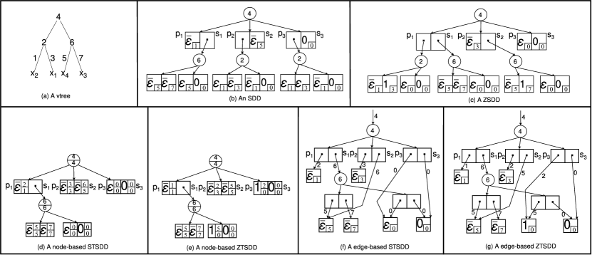
Figure 1: The vtree and the SDD, ZSDD and TSDD representations of the combination set $\{\!\{x_{1},\!x_{2},\!x_{3},\!x_{4}\},\!\{x_{2},\!x_{3},\!x_{4}\},\!\{x_{1},\!x_{3},\!x_{4}\},\!\{x_{1},\!x_{4}\}\!\}$.

Throughout this paper, we use lower case letters (e.g., $x_{1},x_{2}$) for variables, and bold upper case letters (e.g., $\mathbf{X},\mathbf{Y}$) for sets of variables. For a variable $x$, we use $\overline{x}$ to denote the negation of $x$. A literal is a variable or a negated one. A truth assignment over $\mathbf{X}$ is a mapping $\sigma:\mathbf{X}\mapsto\{0,1\}$. We let $\Sigma_{\mathbf{X}}$ be the set of truth assignments over $\mathbf{X}$. We say $f$ is a Boolean function over $\mathbf{X}$, which is a mapping: $\Sigma_{\mathbf{X}}\mapsto\{0,1\}$. We use $\mathbf{1}$ (resp. $\mathbf{0}$) for the Boolean function that maps all assignments to $1$ (resp. $0$). A combination $\widetilde{\mathbf{X}}$ on $\mathbf{X}$ is a subset of $\mathbf{X}$. Every combination $\widetilde{\mathbf{X}}$ corresponds to exactly one truth assignment $\sigma$, that is, $x\in\widetilde{\mathbf{X}}$ iff $\sigma(x)=1$. A combination set $\mathbf{Q}$ over $\mathbf{X}$ is a collection of combinations on $\mathbf{X}$. It was shown that every combination set can be transformed into a Boolean function, and vice versa [8, 17]. The operations on combination sets include: union $\cup$, intersection $\cap$, difference $\setminus$, orthogonal join $\sqcup$ and change [17]. The definitions of the above operations are illustrated in Table I. We use $\mathbf{U}_{\mathbf{X}}$ for the universe set of combinations on $\mathbf{X}$. For example, $\mathbf{U}_{\{x_{1},x_{2}\}}=\{\{x_{1},x_{2}\},\{x_{1}\},\{x_{2}\},\emptyset\}$. We remark that $\mathbf{U}_{\emptyset}=\{\emptyset\}$.

TABLE I: Operations on combination sets.

Operation	Description	Definition
$\mathbf{Q}\cap\mathbf{Q}^{\prime}$	intersection	$\{\widetilde{\mathbf{X}}\mid\widetilde{\mathbf{X}}\in\mathbf{Q}\text{ and }\widetilde{\mathbf{X}}\in\mathbf{Q}^{\prime}\}$
$\mathbf{Q}\cup\mathbf{Q}^{\prime}$	union	$\{\widetilde{\mathbf{X}}\mid\widetilde{\mathbf{X}}\in\mathbf{Q}\text{ or }\widetilde{\mathbf{X}}\in\mathbf{Q}^{\prime}\}$
$\mathbf{Q}\setminus\mathbf{Q}^{\prime}$	difference	$\{\widetilde{\mathbf{X}}\mid\widetilde{\mathbf{X}}\in\mathbf{Q}\text{ and }\widetilde{\mathbf{X}}\notin\mathbf{Q}^{\prime}\}$
$\mathbf{Q}\sqcup\mathbf{Q}^{\prime}$	orthogonal join	$\{\widetilde{\mathbf{X}}\cup\widetilde{\mathbf{X}}^{\prime}\mid\widetilde{\mathbf{X}}\in\mathbf{Q}\text{ and }\widetilde{\mathbf{X}}^{\prime}\in\mathbf{Q}^{\prime}\}$
${\tt Change}(\mathbf{Q},x)$	change	$\{\widetilde{\mathbf{X}}\cup\{x\}\mid\widetilde{\mathbf{X}}\in\mathbf{Q}\text{ and }x\notin\widetilde{\mathbf{X}}\}\cup$
		$\{\widetilde{\mathbf{X}}\setminus\{x\}\mid\widetilde{\mathbf{X}}\in\mathbf{Q}\text{ and }x\in\widetilde{\mathbf{X}}\}$

Let $\mathbf{X}$ and $\mathbf{Y}$ be two disjoint and non-empty sets of variables. We say the set $\{(\mathbf{P}_{1},\mathbf{S}_{1}),\cdots,(\mathbf{P}_{n},\mathbf{S}_{n})\}$ is an $(\mathbf{X},\mathbf{Y})$-decomposition of a combination set $\mathbf{Q}$, iff $\mathbf{Q}=[\mathbf{P}_{1}\sqcup\mathbf{S}_{1}]\cup\cdots\cup[\mathbf{P}_{n}\sqcup\mathbf{S}_{n}]$ where every $\mathbf{P}_{i}$ (resp. $\mathbf{S}_{i}$) is a combination set over $\mathbf{X}$ (resp. $\mathbf{Y}$). A decomposition is compressed iff $\mathbf{S}_{i}\neq\mathbf{S}_{j}$ for $i\neq j$. An $(\mathbf{X},\mathbf{Y})$-decomposition is called an $(\mathbf{X},\mathbf{Y})$-partition, iff (1) every $\mathbf{P}_{i}$ is non-empty, (2) $\mathbf{P}_{i}\cap\mathbf{P}_{j}=\emptyset$ for $i\neq j$, and (3) $\mathbf{P}_{i}\cup\cdots\cup\mathbf{P}_{n}=\mathbf{U}_{\mathbf{X}}$.

A vtree is a full binary tree whose leaves are labeled by variables, which generalizes variable orders. For a vtree $\mathbf{T}$, we use $v(\mathbf{T})$ for the set of variables appearing in leaves of $\mathbf{T}$, and $\mathbf{T}_{l}$ and $\mathbf{T}_{r}$ for the left and right subtrees of $\mathbf{T}$ respectively. There is a special leaf node labeled by $0$ that can be considered as a child of any vtree node and $v(0)=\emptyset$. The notation $\mathbf{T}^{1}\preccurlyeq\mathbf{T}^{2}$ denotes that $\mathbf{T}^{1}$ is a subtree of $\mathbf{T}^{2}$ and $\mathbf{T}^{1}\prec\mathbf{T}^{2}$ means that $\mathbf{T}^{1}$ is a proper subtree.

Based the notion of vtrees, a combination set can be graphically represented by a structured decomposable diagram[18].

Definition 1

A structured decomposable diagram is a pair $(\mathbf{T},\alpha)$ where $\mathbf{T}$ is a vtree and $\alpha$ is recursively defined as follows

• $\alpha$ is a terminal node labeled by one of the four symbols: $\mathbf{1}$, $\mathbf{0}$, $\varepsilon$ and $\bar{\varepsilon}$, and $\mathbf{T}$ is any vtree.

• $\alpha$ is a decomposition node $\{(p_{1},s_{1}),\cdots,(p_{n},s_{n})\}$ satisfying the following conditions:

  1. each $p_{i}$ is a structured decomposable diagram $(\mathbf{T}_{i}^{1},\beta)$ where $\mathbf{T}_{i}^{1}\preccurlyeq\mathbf{T}_{l}$;

  2. each $s_{i}$ is a structured decomposable diagram $(\mathbf{T}_{i}^{2},\gamma)$ where $\mathbf{T}_{i}^{2}\preccurlyeq\mathbf{T}_{r}$.

Every pair $(p_{i},s_{i})$ of a decomposition node is called an element where $p_{i}$ is called a prime and $s_{i}$ is called a sub.

We hereafter provide two ways to interpret a structured decomposable diagram $(\mathbf{T}^{2},\alpha)$ as a combination set, which we call standard and zero-suppressed semantics. Since the standard semantics depends on an extra vtree $\mathbf{T}^{1}$, it is a mapping from structured decomposable diagrams and vtrees into combination sets.

Definition 2

Let $\mathbf{T}^{1}$ be a vtree and $(\mathbf{T}^{2},\alpha)$ be a structured decomposable diagram where $\mathbf{T}^{2}\preccurlyeq\mathbf{T}^{1}$. The standard semantics $\langle\mathbf{T}^{1},(\mathbf{T}^{2},\alpha)\rangle_{s}$ is recursively defined as follows:

• $\langle\mathbf{T}^{1},(\mathbf{T}^{2},\mathbf{1})\rangle_{s}=\mathbf{U}_{\mathbf{T}^{1}}$ and $\langle\mathbf{T}^{1},(\mathbf{T}^{2},\mathbf{0})\rangle_{s}=\emptyset$;

• $\langle\mathbf{T}^{1},(\mathbf{T}^{2},\varepsilon)\rangle_{s}=\mathbf{U}_{v(\mathbf{T}^{1})\setminus v(\mathbf{T}^{2})}$ and $\langle\mathbf{T}^{1},(\mathbf{T}^{2},\bar{\varepsilon})\rangle_{s}=\mathbf{U}_{v(\mathbf{T}^{1})\setminus v(\mathbf{T}^{2})}\sqcup(\mathbf{U}_{v(\mathbf{T}^{2})}\setminus\{\emptyset\})$;

• $\langle\mathbf{T}^{1},(\mathbf{T}^{2},\{(p_{1},s_{1}),\cdots,(p_{n},s_{n})\})\rangle_{s}=\mathbf{U}_{v(\mathbf{T}^{1})\setminus v(\mathbf{T}^{2})}\sqcup\left[\bigcup\limits_{i=1}\limits^{n}(\langle\mathbf{T}_{l}^{2},p_{i}\rangle_{s}\sqcup\langle\mathbf{T}_{r}^{2},s_{i}\rangle_{s})\right]$.

The standard semantics $\langle\mathbf{T}^{1},(\mathbf{T}^{2},\alpha)\rangle_{s}$ contains two combination sets. The main combination set is based on $\mathbf{T}^{2}$ and $\alpha$. The four terminal nodes $\mathbf{1}$, $\mathbf{0}$, $\varepsilon$ and $\bar{\varepsilon}$ represent $\mathbf{U}_{v(\mathbf{T}^{2})}$, $\emptyset$, $\{\emptyset\}$ and $\mathbf{U}_{v(\mathbf{T}^{2})}\setminus\{\emptyset\}$, respectively. The decomposition node $\{(p_{1},s_{1}),\cdots,(p_{n},s_{n})\}$ denotes the combination set that is the union of the orthogonal join of $\langle p_{i}\rangle_{s}$ and $\langle s_{i}\rangle_{s}$ for every pair $(p_{i},s_{i})$. The auxiliary combination set is the universe set over $v(\mathbf{T}^{1})\setminus v(\mathbf{T}^{2})$. The standard semantics is the orthogonal join of main and auxiliary combination sets. For example, the combination set of $(\mathbf{T}^{1},\mathbf{T}^{2},\mathbf{1})$ is $\mathbf{U}_{v(\mathbf{T}^{2})}\sqcup\mathbf{U}_{v(\mathbf{T}^{1})\setminus v(\mathbf{T}^{2})}$, and hence being $\mathbf{U}_{v(\mathbf{T}^{1})}$.

The zero-suppressed semantics $\langle\mathbf{T}^{1},(\mathbf{T}^{2},\alpha)\rangle_{z}$ is only the main combination set, which can be easily defined. For example, $\langle\mathbf{T}^{1},(\mathbf{T}^{2},\{(p_{1},s_{1}),\cdots,(p_{n},s_{n})\})\rangle_{z}=\bigcup\limits_{i=1}\limits^{n}(\langle p_{i}\rangle_{s}\sqcup\langle s_{i}\rangle_{s})$. We introduce the extra vtree $\mathbf{T}^{1}$ in the zero-suppressed semantics in accordance with the standard semantics though it is not required for the zero-suppressed semantics.

Based on the standard semantics, we impose some restrictions on structured decomposable diagram and obtain the definition of sentenial decision diagram (SDD).

Definition 3

A structured decomposable diagram $(\mathbf{T},\alpha)$ is a sentenial decision diagram, if one of the following holds:

1. $\alpha$ is a terminal node labeled by $\mathbf{1}$ or $\mathbf{0}$, and $\mathbf{T}=0$.

2. $\alpha$ is a terminal node labeled by $\varepsilon$ or $\bar{\varepsilon}$, and $\mathbf{T}$ is a leaf node.

3. $\alpha$ is a decomposition node $\{(p_{1},s_{1}),\cdots,(p_{n},s_{n})\}$, and all of the following hold:

   • $\langle\mathbf{T}_{l},p_{i}\rangle_{s}\neq\emptyset$ for $1\leq i\leq n$;

   • $\langle\mathbf{T}_{l},p_{i}\rangle_{s}\cap\langle\mathbf{T}_{l},p_{j}\rangle_{s}=\emptyset$ for $i\neq j$;

   • $\bigcup\limits_{i=1}^{n}\langle\mathbf{T}_{l},p_{i}\rangle_{s}=\mathbf{U}_{v(\mathbf{T}_{l})}$.

The definition of zero-suppressed sentenial decision diagram (ZSDD) is the same as SDD, except that (1) we require $\mathbf{T}$ to be the special vtree $0$ when $\alpha$ is a terminal node labeled by $\varepsilon$; (2) the vtree $\mathbf{T}$ can be any leaf node when $\alpha$ is labeled by $\mathbf{1}$; (3) we use the zero-suppressed semantics for the decomposition node.

An SDD can be transformed to an equivalent one with smaller size by the following the standard compressness and trimming rules.

• Standard compression rule (S-compression rule): if $\langle\mathbf{T}_{r},s_{i}\rangle_{s}=\langle\mathbf{T}_{r},s_{j}\rangle_{s}$, then replace $(\mathbf{T},\{(p_{1},s_{1}),\cdots,(p_{i},s_{i}),\\ \cdots,(p_{j},s_{j}),\cdots,(p_{n},s_{n})\})$ with $(\mathbf{T},\{(p_{1},s_{1}),\cdots,(p^{\prime},s_{i}),\\ \cdots,(p_{n},s_{n})\})$ where $\langle\mathbf{T}_{l},p^{\prime}\rangle_{s}=\langle\mathbf{T}_{l},p_{i}\rangle_{s}\cup\langle\mathbf{T}_{l},p_{j}\rangle_{s}$.

• Standard trimming rule (S-trimming rule):

  1. replace the diagram $(\mathbf{T},\{(p,s)\})$ by the diagram $s$.

  2. if $\langle\mathbf{T}_{r},s_{1}\rangle_{s}=\mathbf{U}_{v(\mathbf{T}_{r})}$ and $\langle\mathbf{T}_{r},s_{2}\rangle_{s}=\emptyset$, then replace the diagram $(\mathbf{T},\{(p_{1},s_{1}),(p_{2},s_{2})\})$ by the diagram $p_{1}$.

The S-compression rule combines two elements $(p_{i},s_{i})$ and $(p_{j},s_{j})$ when $s_{i}$ and $s_{j}$ denotes the same combination set. The two S-trimming rules aim to remove the universe set over a subset of variables in a decomposition node. By repeatedly applying the S-compression and trimming rules, we can create the unique SDD.

Similarly, we can define the zero-suppressed compression and trimming rules for ZSDD.

• Zero-suppressed compression rule (Z-compression rule): if $\langle\mathbf{T}_{r},s_{i}\rangle_{z}=\langle\mathbf{T}_{r},s_{j}\rangle_{z}$, then replace $(\mathbf{T},\{(p_{1},s_{1}),\cdots,(p_{i},s_{i}),\\ \cdots,(p_{j},s_{j}),\cdots,(p_{n},s_{n})\})$ with $(\mathbf{T},\{(p_{1},s_{1}),\cdots,(p^{\prime},s_{i}),\\ \cdots,(p_{n},s_{n})\})$ where $\langle\mathbf{T}_{l},p^{\prime}\rangle_{z}=\langle\mathbf{T}_{l},p_{i}\rangle_{z}\cup\langle\mathbf{T}_{l},p_{j}\rangle_{z}$.

• Zero-suppressed trimming rule (Z-trimming rule):

  1. if $\langle\mathbf{T}_{l},p_{1}\rangle_{z}=\{\emptyset\}$ (resp. $\langle\mathbf{T}_{r},s_{1}\rangle_{z}=\{\emptyset\}$) and $\langle\mathbf{T}_{r},s_{2}\rangle_{z}=\emptyset$, then replace the diagram $(\mathbf{T},\{(p_{1},s_{1}),(p_{2},s_{2})\})$ by the diagram $s_{1}$ (resp. $p_{1}$);

  2. if $\langle\mathbf{T}_{r},s\rangle_{z}=\emptyset$, then replace the diagram $(\mathbf{T},\{(p,s)\})$ by the diagram $s$;

The Z-compression rule is similar to the S-compression rule except that it uses the zero-suppressed semantics. The two Z-trimming rules seek to eliminate $\{\emptyset\}$. We acquire the canonical representation via utilizing the Z-trimming rule on ZSDDs.

Example 1

Fig. 1(a) shows the vtree $\mathbf{T}$ where its left subtree $\mathbf{T}_{l}$ involves $\mathbf{X}:\{x_{1},x_{2}\}$ while its right one $\mathbf{T}_{r}$ involves $\mathbf{Y}:\{x_{3},x_{4}\}$. Fig. 1(b) depicts an SDD representing the combination set $\mathbf{Q}=\{\{x_{1},x_{2},x_{3},x_{4}\},\{x_{2},x_{3},x_{4}\},\{x_{1},x_{3},x_{4}\},\{x_{1},x_{4}\}\}$ based on $\mathbf{T}$. The $(\mathbf{X},\mathbf{Y})$-partition of $\mathbf{Q}$ contains three elements: $(\overbrace{\{\{x_{1},x_{2}\},\{x_{2}\}\}}^{\mathbf{P}_{1}},\overbrace{\{\{x_{3},x_{4}\}\}}^{\mathbf{S}_{1}})$, $(\overbrace{\{\{x_{1}\}\}}^{\mathbf{P}_{2}},\overbrace{\{\{x_{3},x_{4}\},\{x_{4}\}\}}^{\mathbf{S}_{2}})$ and $(\overbrace{\{\emptyset\}}^{\mathbf{P}_{3}},\overbrace{\emptyset}^{\mathbf{S}_{3}})$. Each combination subset $\mathbf{P}_{i}$ (resp. $\mathbf{S}_{i}$) corresponds to the node $p_{i}$ (resp. $s_{i}$) of the SDD. The ZSDD representation for $\mathbf{Q}$ with smaller nodes than the SDD one is shown in Fig. 1(c). ∎

III Tagged Sentential Decision Diagrams

In this section, we will first provide a general structure, namely extended structured decomposable diagram (ESDD), that is, the syntactic definition for TSDDs, and then with two different semantics, that are, a mapping from ESDDs to combination sets. The ESDD with the standard semantics is called standard TSDD (STSDD) while it is called zero-suppressed TSDD (ZTSDD) under the zero-suppressed semantics. We also present the trimming rules for STSDD so as to reduce the size of STSDD and obtain the canonicity theorem of STSDDs. Finally, we provide two implementations for TSDDs: node-based and edge-based. Hence, we obtain four versions of TSDDs.

III-A The Syntax and semantics

In order to facilitate combining two types of trimming rules, we first provide a general structure, namely extended structured decomposable diagram (ESDD).

(a) A terminal node

(b) A decomposition node

Figure 2: Two types of nodes of ESDDs

Definition 4

An ESDD is a tuple $(\mathbf{T}^{1},\mathbf{T}^{2},\alpha)$ s.t. $\mathbf{T}^{2}\preccurlyeq\mathbf{T}^{1}$, which is recursively defined as:

• $\alpha$ is a terminal node labeled by one of the four symbols: $\mathbf{1}$, $\mathbf{0}$, $\varepsilon$ and $\bar{\varepsilon}$;

• $\alpha$ is a decomposition node $\{(p_{1},s_{1}),\cdots,(p_{n},s_{n})\}$ satisfying the following:

  • each $p_{i}$ is an ESDD $(\mathbf{T}^{3},\mathbf{T}^{4},\beta)$ where $\mathbf{T}^{4}\preccurlyeq\mathbf{T}^{3}\prec\mathbf{T}^{2}$;

  • each $s_{i}$ is an ESDD $(\mathbf{T}^{5},\mathbf{T}^{6},\gamma)$ where $\mathbf{T}^{6}\preccurlyeq\mathbf{T}^{5}\prec\mathbf{T}^{2}$.

An ESDD $F=(\mathbf{T}^{1},\mathbf{T}^{2},\alpha)$ consists of three components: the primary vtree $\mathbf{T}^{1}$, the secondary vtree $\mathbf{T}^{2}$ and the terminal (or decomposition) node $\alpha$. As seen in Fig. 2(a), when $\alpha$ is a terminal node, the above three components are represented by a square where $\alpha$ is shown in the left side of the square, $\mathbf{T}^{1}$ in the upper-right corner and $\mathbf{T}^{2}$ in the lower-right corner. When $\alpha$ is a decomposition node, the primary and secondary vtrees are displayed as a circle with outgoing edges pointing to the elements as shown in Fig. 2(b). Each element $(p_{i},s_{i})$ is represented by a paired box where the left box represents the prime $p_{i}$ and the right box stands for the sub $s_{i}$. We use $pv(F)$ for the primary vtree of $F$ and $sv(F)$ for the secondary vtree. The size of $\alpha$, denoted by $|\alpha|$, is the sizes of all of its decompositions.

To interpret ESDDs, we provide the semantics, that is, a mapping from ESDDs into combination sets.

Definition 5

Let $(\mathbf{T}^{1},\mathbf{T}^{2},\alpha)$ be an ESDD. The standard semantics $\lVert(\mathbf{T}^{1},\mathbf{T}^{2},\alpha)\rVert_{s}$ is recursively defined as:

• $\lVert(\mathbf{T}^{1},\mathbf{T}^{2},\mathbf{1})\rVert_{s}=\mathbf{U}_{v(\mathbf{T}^{1})}$ and $\lVert(\mathbf{T}^{1},\mathbf{T}^{2},\mathbf{0})\rVert_{s}=\emptyset$;

• $\lVert(\mathbf{T}^{1},\mathbf{T}^{2},\varepsilon)\rVert_{s}=\mathbf{U}_{v(\mathbf{T}^{1})\setminus v(\mathbf{T}^{2})}$ and $\lVert(\mathbf{T}^{1},\mathbf{T}^{2},\bar{\varepsilon})\rVert_{s}=\mathbf{U}_{v(\mathbf{T}^{1})\setminus v(\mathbf{T}^{2})}\sqcup(\mathbf{U}_{v(\mathbf{T}^{2})}\setminus\{\emptyset\})$;

• $\lVert(\mathbf{T}^{1},\mathbf{T}^{2},\{(p_{1},s_{1}),\cdots,(p_{n},s_{n})\})\rVert_{s}=\mathbf{U}_{v(\mathbf{T}^{1})\setminus v(\mathbf{T}^{2})}\sqcup\left[\bigcup\limits_{i=1}\limits^{n}(\lVert p_{i}\rVert_{s}\sqcup\lVert s_{i}\rVert_{s})\right]$.

Since every ESDD involves an extra vtree $\mathbf{T}^{1}$ compared to structured decision diagrams, the standard semantics for ESDDs is similar to structured decision diagrams (cf. Definition 2).

A standard tagged sentential decision diagram (STSDD) is an ESDD with the following constraints.

Definition 6

An ESDD $(\mathbf{T}^{1},\mathbf{T}^{2},\alpha)$ is an STSDD, if one of the following holds:

• $\alpha$ is a terminal node labeled by $\mathbf{0}$ and $\mathbf{T}^{1}=\mathbf{T}^{2}=0$.

• $\alpha$ is a terminal node labeled by $\varepsilon$ and $\mathbf{T}^{2}=0$.

• $\alpha$ is a terminal node labeled by $\bar{\varepsilon}$ and $\mathbf{T}^{2}$ is a leaf node.

• $\alpha$ is a decomposable node $\{(p_{1},s_{1}),\cdots,(p_{n},s_{n})\}$ and $\{(\lVert p_{1}\rVert_{s},\lVert s_{1}\rVert_{s}),\cdots,(\lVert p_{n}\rVert_{s},\lVert s_{n}\rVert_{s})\}$ is an $(\mathbf{X},\mathbf{Y})$-partition where $\mathbf{X}=v(\mathbf{T}^{2}_{l})$ and $\mathbf{Y}=v(\mathbf{T}^{2}_{r})$.

We remark that we use the terminal node $\varepsilon$ instead of $\mathbf{1}$ in STSDDs since $\lVert(\mathbf{T}^{1},\mathbf{T}^{2},\mathbf{1})\rVert_{s}=\lVert(\mathbf{T}^{1},0,\varepsilon)\rVert_{s}$ for any vtrees $\mathbf{T}^{1}$ and $\mathbf{T}^{2}$.

III-B Canonicity

We hereafter design the standard tagged compression and trimming rules for reducing the size of STSDD and obtaining the canonicity property of STSDDs.

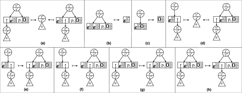
Figure 3: Trimming rules for STSDD

• Standard tagged compression rule (ST-compression rule):
  if $\lVert s_{i}\rVert_{s}=\lVert s_{j}\rVert_{s}$, then replace $(\mathbf{T}^{1},\mathbf{T}^{2},\{(p_{1},s_{1}),\cdots,(p_{i},s_{i}),\cdots,(p_{j},s_{j}),\cdots,(p_{n},s_{n})\})$ with $(\mathbf{T}^{1},\mathbf{T}^{2},\{(p_{1},s_{1}),\cdots,(p_{i}^{\prime},s_{i}),\cdots,(p_{n},s_{n})\})$ where $\lVert p_{i}^{\prime}\rVert_{s}=\lVert p_{i}\rVert_{s}\cup\lVert p_{j}\rVert_{s}$.

• Standard tagged trimming rule (ST-trimming rule) (Fig 3):

  1. if $p_{1}=(\mathbf{T}^{2},\mathbf{T}^{3},\alpha)$, $\lVert s_{1}\rVert_{s}=\{\emptyset\}$ and $\lVert s_{2}\rVert_{s}=\emptyset$, or $\lVert p_{1}\rVert_{s}=\{\emptyset\}$, $s_{1}=(\mathbf{T}^{2},\mathbf{T}^{3},\alpha)$ and $\lVert s_{2}\rVert_{s}=\emptyset$, then replace $(\mathbf{T}^{1},\mathbf{T}^{1},\{(p_{1},s_{1}),(p_{2},s_{2})\})$ with $(\mathbf{T}^{2},\mathbf{T}^{3},\alpha)$;

  2. if $\lVert p_{1}\rVert_{s}=\lVert s_{1}\rVert_{s}=\{\emptyset\}$, $\lVert s_{2}\rVert_{s}=\emptyset$ and $\mathbf{T}^{2}$ is $\mathbf{T}^{1}_{l}$ or $\mathbf{T}^{1}_{r}$, then replace $(\mathbf{T}^{1},\mathbf{T}^{2},\{(p_{1},s_{1}),$ $(p_{2},s_{2})\})$ with $(\mathbf{T}^{3},0,\varepsilon)$, where $\mathbf{T}^{3}\!=\!\mathbf{T}^{1}_{l}$ when $\mathbf{T}^{2}\!=\!\mathbf{T}^{1}_{l}$ and $\mathbf{T}^{3}\!=\!\mathbf{T}^{1}_{r}$ when $\mathbf{T}^{2}\!=\!\mathbf{T}^{1}_{r}$.

  3. if $p=(\mathbf{T}^{2}_{l},0,\varepsilon)$ and $\lVert s\rVert_{s}=\emptyset$, then replace $(\mathbf{T}^{1},\mathbf{T}^{2},\{(p,s)\})$ with $(0,0,\mathbf{0})$.

  4. if $p_{1}=(\mathbf{T}^{2}_{l},\mathbf{T}^{3},\alpha)$, $s_{1}=(\mathbf{T}_{r}^{2},0,\varepsilon)$ and $\lVert s_{2}\rVert_{s}=\emptyset$ (resp.
     $p=(\mathbf{T}^{2}_{l},0,\varepsilon)$ and $s=(\mathbf{T}^{2}_{r},\mathbf{T}^{3},\alpha)$), then replace $(\mathbf{T}^{1},\mathbf{T}^{2}_{r},\{((0,0,\varepsilon),s_{1}),(p_{2},(0,0,\mathbf{0}))\})$ (resp. $(\mathbf{T}^{1},\mathbf{T}^{2},\{(p,s)\})$) with $(\mathbf{T}^{1},\mathbf{T}^{3},\alpha)$;

  5. if $p_{1}=(\mathbf{T}^{2}_{l},0,\varepsilon)$, $s_{1}=(\mathbf{T}^{3},\mathbf{T}^{4},\alpha)$ and $\mathbf{T}^{3}\preccurlyeq(\mathbf{T}^{2}_{r})_{l}$, then
     replace $(\mathbf{T}^{1},\mathbf{T}^{2},\{(p_{1},s_{1})\})$ with $(\mathbf{T}^{1},\mathbf{T}^{2}_{r},\{(s_{1},(0,0,\varepsilon)),\\ (p_{2},(0,0,\mathbf{0}))\})$ where $\lVert p_{2}\rVert_{s}=\mathbf{U}_{(\mathbf{T}^{2}_{r})_{l}}\setminus\lVert s_{1}\rVert_{s}$;

  6. if $p_{1}=(\mathbf{T}^{2}_{l},0,\varepsilon)$, $s_{1}=(\mathbf{T}^{3},\mathbf{T}^{4},\alpha)$ and $\mathbf{T}^{3}\preccurlyeq(\mathbf{T}^{2}_{r})_{r}$, then
     replace $(\mathbf{T}^{1},\mathbf{T}^{2},\{(p_{1},s_{1})\})$ with $(\mathbf{T}^{1},\mathbf{T}^{2}_{r},\{((0,0,\varepsilon),s_{1}),\\ (p_{2},(0,0,\mathbf{0}))\})$ where $\lVert p_{2}\rVert_{s}=\mathbf{U}_{(\mathbf{T}^{2}_{r})_{l}}\setminus\{\emptyset\}$;

  7. if $p_{1}=(\mathbf{T}^{3},\mathbf{T}^{4},\alpha)$, $s_{1}=(\mathbf{T}_{r}^{2},0,\varepsilon)$, $\lVert s_{2}\rVert_{s}=\emptyset$ and $\mathbf{T}^{3}\preccurlyeq(\mathbf{T}^{2}_{l})_{l}$,then replace $(\mathbf{T}^{1},\mathbf{T}^{2},\{(p_{1},s_{1}),(p_{2},s_{2})\})$ with $(\mathbf{T}^{1},\!\mathbf{T}_{l}^{2},\!{(p_{1},(0,0,\varepsilon)),\!(p_{3},\!s_{2})})$ where $\!\lVert p_{3}\rVert_{s}\!=\!\mathbf{U}_{(\mathbf{T}^{2}_{l})_{l}}\!\setminus\lVert p_{1}\rVert_{s}$;

  8. if $p_{1}=(\mathbf{T}^{3},\mathbf{T}^{4},\alpha)$, $s_{1}=(\mathbf{T}_{r}^{2},0,\varepsilon)$, $\lVert s_{2}\rVert_{s}=\emptyset$ and $\mathbf{T}^{3}\preccurlyeq(\mathbf{T}^{2}_{l})_{r}$, then replace $(\mathbf{T}^{1},\mathbf{T}^{2},\{(p_{1},s_{1}),(p_{2},s_{2})\})$ with $(\mathbf{T}^{1},\!\mathbf{T}^{2}_{l},\!\{((0,0,\varepsilon),\!p_{1}),(p_{3},\!s_{2})\})$ where $\!\lVert p_{3}\rVert_{s}\!=\!\mathbf{U}_{(\mathbf{T}^{2}_{l})_{l}}\!\setminus\!\{\emptyset\}$.

The goal of ST-compression rule is to combine elements with the same subs. The ST-trimming rules are shown in Fig. 3. Rules (a) and (b) are used to eliminate the sub-diagram representing the set $\{\emptyset\}$ whereas rules (c) – (h) aim to reduce the sub-diagram denoting the universe set over a subset of variables. A STSDD is compressed (resp. trimmed), if no ST-compression (resp. trimming) rule can be applied in it. We hereafter state the important property of compressed and trimmed STSDDs.

Theorem 1

Given a vtree $\mathbf{T}$ over $\mathbf{X}$, for any combination set $\mathbf{Q}$ over $\mathbf{X}$, there is a unique compressed and trimmed STSDD $(\mathbf{T}^{1},\mathbf{T}^{2},\alpha)$ s.t. $\mathbf{T}^{1}\preccurlyeq\mathbf{T}$ and $\lVert(\mathbf{T}^{1},\mathbf{T}^{2},\alpha)\rVert_{s}=\mathbf{Q}$.

Thanks to the additional vtree and the above trimming rules, STSDD has compactness advantages over both SDD and ZSDD.

Example 2

We continue to Example 1. The combination set $\mathbf{Q}$ in SDD, ZSDD and STSDD representations are shown in Fig. 1(b) – (d), respectively. The combination subsets $\mathbf{P}_{1}$, $\mathbf{S}_{2}$ and $\mathbf{S}_{3}$ can be represented as terminal nodes in SDD while $\mathbf{P}_{2}$, $\mathbf{P}_{3}$ and $\mathbf{S}_{3}$ can be in ZSDD. Hence, the combination set has SDD and ZSDD representations of size $9$. All of the above $5$ combination subsets are represented by terminal nodes in STSDD. The STSDD representation, in comparison, is only $5$ in size smaller than SDD and ZSDD. ∎

III-C Zero-suppressed Variant

In a STSDD $(\mathbf{T}^{1},\mathbf{T}^{2},\alpha)$, S-trimming rules are applied from the primary vtree $\mathbf{T}^{1}$ to the secondary one $\mathbf{T}^{2}$ and Z-trimming rules are applied from the secondary vtree $\mathbf{T}^{2}$ to the primary vtree of each of the terminal node $\alpha$, or the prime $p_{i}$ and the sub $s_{i}$ of the decomposition node $\alpha$. We hereafter define a variant of STSDD by reversing the order of trimming rules, that is, Z-trimming rules are implied first and S-trimming rules second.

Definition 7

Let $(\mathbf{T}^{1},\mathbf{T}^{2},\alpha)$ be an ESDD. The zero-suppressed semantics $\lVert(\mathbf{T}^{1},\mathbf{T}^{2},\alpha)\rVert_{z}$ is recursively defined as:

• $\lVert(\mathbf{T}^{1},\mathbf{T}^{2},\mathbf{1})\rVert_{z}=\mathbf{U}_{v(\mathbf{T}^{2})}$ and $\lVert(\mathbf{T}^{1},\mathbf{T}^{2},\mathbf{0})\rVert_{z}=\emptyset$;

• $\lVert(\mathbf{T}^{1},\mathbf{T}^{2},\varepsilon)\rVert_{z}=\{\emptyset\}$ and $\lVert(\mathbf{T}^{1},\mathbf{T}^{2},\bar{\varepsilon})\rVert_{z}=\mathbf{U}_{v(\mathbf{T}^{2})}\setminus\{\emptyset\}$;

• $\lVert(\mathbf{T}^{1},\mathbf{T}^{2},\{(p_{1},s_{1}),\cdots,(p_{n},s_{n})\})\rVert_{z}=\\ \bigcup\limits_{i=1}\limits^{n}\left[\mathbf{U}_{v(\mathbf{T}^{2})\setminus(pv(p_{i})\cup pv(s_{i}))}\sqcup\lVert p_{i}\rVert_{z}\sqcup\lVert s_{i}\rVert_{z}\right]$.

When $\alpha$ is the terminal node, the zero-suppressed semantics is only the main combination set of $\alpha$. When $\alpha$ is the decomposition node, besides the main combination set, the zero-suppressed semantics contains an extra combination set, that is, the universal set of $v(\mathbf{T}^{2})\setminus(pv(p_{i})\cup pv(s_{i}))$ for each element $(p_{i},s_{i})$.

Based on the zero-suppressed semantics, we provide the zero-suppressed variant of TSDD, namely zero-suppressed TSDD (ZTSDD).

Definition 8

An ESDD $(\mathbf{T}^{1},\mathbf{T}^{2},\alpha)$ is an ZTSDD, if one of the following holds:

• $\alpha$ is a terminal node labeled by $\mathbf{0}$ and $\mathbf{T}^{1}=\mathbf{T}^{2}=0$.

• $\alpha$ is a terminal node labeled by $\mathbf{1}$ and $\mathbf{T}^{2}=0$.

• $\alpha$ is a terminal node labeled by $\bar{\varepsilon}$ and $\mathbf{T}^{2}$ is a leaf node.

• $\alpha$ is a decomposable node $\{(p_{1},s_{1}),\cdots,(p_{n},s_{n})\}$ and $\{(\lVert p_{1}\rVert_{z},\lVert s_{1}\rVert_{z}),\cdots,(\lVert p_{n}\rVert_{z},\lVert s_{n}\rVert_{z})\}$ is an $(\mathbf{X},\mathbf{Y})$-partition where $\mathbf{X}=v(\mathbf{T}^{2}_{l})$ and $\mathbf{Y}=v(\mathbf{T}^{2}_{r})$.

We remark that the terminal node $\varepsilon$ is omitted in ZTSDD due to the fact that $\lVert(\mathbf{T}^{1},\mathbf{T}^{2},\varepsilon)\rVert_{z}=\lVert(\mathbf{T}^{1},0,\mathbf{1})\rVert_{z}$ for any vtrees $\mathbf{T}^{1}$ and $\mathbf{T}^{2}$. In addition, ZTSDD is a canonical form for combination set by applying zero-suppressed tagged compression and trimming rules.

Fig. 1(e) shows the ZTSDD for representing the example. Since ZTSDD both enjoy the advantages of SDD and ZSDD, it has smaller size $5$ than SDD and ZSDD, which is the same as STSDD. We remark that ZTSDDs and STSDDs in general have different sizes for representing the same combination set given the same vtree.

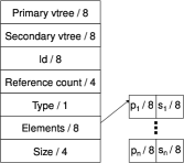
(a) Node-based TSDD node

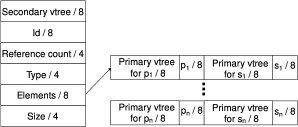
(b) Edge-based TSDD node

Figure 4: Two implementations for TSDDs

III-D Edge-based Variant

In Definition 6, both the primary vtree $\mathbf{T}^{1}$ and the secondary one $\mathbf{T}^{2}$ are kept in each TSDD node. Such TSDD node is called node-based TSDD node. We now introduce the edge-based variant of TSDD. The main distinctions between node-based and edge-based TSDD are: (1) Each edge-based TSDD node only includes the secondary vtree $\mathbf{T}^{2}$ and the terminal/decomposition node $\alpha$; (2) Each element of a decomposition node consists of not only the prime $p$ and the sub $s$ but also two vtrees $\mathbf{T}_{p}$ and $\mathbf{T}_{s}$ that are the primary vtrees of $p$ and $s$, respectively; (3) There is an extra edge pointing to the root node denoting the primary vtree of the root node.

The main data structures of node-based TSDDs and edge-based TSDDs are shown in Fig. 4, respectively. Suppose that the TSDD node has $n$ pairs of primes and subs. We remark that $n=0$ when the node is a terminal node. In the node-based TSDDs, each node requires at least $41+16n$ bytes: $8$ bytes for the pointer to the primary vtree, $8$ bytes for the pointer to the secondary vtree, $8$ bytes for the id of the node in the unique table that ensures no two equivalent TSDD nodes are stored, $4$ bytes for the reference count that is used to garbage collection, $1$ byte for the type of this node: terminal node or decomposition node, $8$ bytes for the pointer to a singly-linked list of pairs of primes nd subs, and $4$ bytes for the number of elements. The node of edge-based TSDD has the similar data structure with node-based TSDD. However, each edge-based TSDD node do not have the primary vtree and each element has two additional primary vtrees for the prime and the sub. The size of a edge-based node is $33+32n$.

Fig. 1(f) and (g) show the edge-based STSDD and ZTSDD representations for the same example. Node-based STSDD representation for $\mathbf{Q}$ needs $449$ bytes whereas that of edge-based one requires $432$ bytes. Due to this sharing mechanism, edge-based variant consumes less memory than node-based one when numerous nodes share the same secondary vtree and terminal (or decomposable) node. Otherwise, node-based variant is a data structure occupying less memory space for storing TSDDs.

IV Operations on STSDD

In this section, we will design the algorithms of STSDDs for achieving the five operations on combination sets. We first introduce a normalization algorithm that serves as the basis of the above algorithms, and then introduce a unified algorithm that accomplishes the three operations: intersection, union and difference, and followed by two algorithms for orthogonal join and change operations.

IV-A Apply

The normalization rules can be considered as a reverse of trimming rules. There are two types of normalization rules. Given a vtree $\mathbf{T}^{3}$ s.t. $\mathbf{T}^{1}\preccurlyeq\mathbf{T}^{3}$, the first one is to transform a STSDD $(\mathbf{T}^{1},\mathbf{T}^{2},\alpha)$ into an equivalent one $(\mathbf{T}^{3},\mathbf{T}^{4},\beta)$, denoted by ${\tt Normalize1}((\mathbf{T}^{1},\mathbf{T}^{2},\alpha),\mathbf{T}^{3})$.

1. if $\mathbf{T}^{1}=\mathbf{T}^{3}$, then $\mathbf{T}^{4}=\mathbf{T}^{2}$ and $\beta=\alpha$.

2. if $\mathbf{T}^{1}\prec\mathbf{T}^{3}_{l}$, then $\mathbf{T}^{4}=\mathbf{T}^{3}$ and $\beta=\{((\mathbf{T}^{1},\mathbf{T}^{2},\alpha),(0,0,\varepsilon)),\\ (p,(0,0,\mathbf{0}))\}$ where $\lVert p\rVert_{s}=\mathbf{U}_{\mathbf{T}^{3}_{l}}\setminus\lVert(\mathbf{T}^{1},\mathbf{T}^{2},\alpha)\rVert_{s}$.

3. if $\mathbf{T}^{1}\prec\mathbf{T}^{3}_{r}$, then $\mathbf{T}^{4}=\mathbf{T}^{3}$ and $\beta=\{((0,0,\varepsilon),(\mathbf{T}^{1},\mathbf{T}^{2},\alpha)),\\ (p,(0,0,\mathbf{0}))\}$ where $\lVert p\rVert_{s}=\mathbf{U}_{\mathbf{T}^{3}_{l}}\setminus\{\emptyset\}$.

The second type of normalization rules takes a STSDD $(\mathbf{T}^{1},\mathbf{T}^{2},\alpha)$ and a vtree $\mathbf{T}^{4}$ where $\mathbf{T}^{2}\preccurlyeq\mathbf{T}^{4}\preccurlyeq\mathbf{T}^{1}$ as input, and outputs the resulting STSDD, denoted by ${\tt Normalize2}((\mathbf{T}^{1},\mathbf{T}^{2},\alpha),\mathbf{T}^{4})$, with the same combination set as $(\mathbf{T}^{1},\mathbf{T}^{2},\alpha)$.

1. if $\mathbf{T}^{2}=\mathbf{T}^{4}$, then $\mathbf{T}^{3}=\mathbf{T}^{1}$ and $\beta=\alpha$.

2. if $\mathbf{T}^{2}\prec\mathbf{T}^{4}_{l}$, then $\mathbf{T}^{3}=\mathbf{T}^{1}$ and $\beta=\{((\mathbf{T}^{4}_{l},\mathbf{T}^{2},\alpha),(\mathbf{T}^{4}_{r},0,\varepsilon)),\\ (p,(0,0,\mathbf{0}))\}$ where $\lVert p\rVert_{s}=\mathbf{U}_{\mathbf{T}^{4}_{l}}\setminus\lVert(\mathbf{T}^{1},\mathbf{T}^{2},\alpha)\rVert_{s}$.

3. if $\mathbf{T}^{2}\!\prec\!\mathbf{T}^{4}_{r}$, then $\mathbf{T}^{3}\!=\!\mathbf{T}^{1}$ and $\beta=\{((\mathbf{T}^{4}_{l},0,\varepsilon),\!(\mathbf{T}^{4}_{r},\mathbf{T}^{2},\alpha))\}$.

Input : $F$: a STSDD $(\mathbf{T}^{1},\mathbf{T}^{2},\alpha)$;

$G$: a STSDD $(\mathbf{T}^{3},\mathbf{T}^{4},\beta)$;

$\circ$: an operator on combination sets ($\cap$, $\cup$ or $\setminus$).

Output : $H$: The resulting STSDD $(\mathbf{T}^{5},\mathbf{T}^{6},\gamma)$.

1

2if Some cases are satisfied then  return predefined results ;

3

4if ${\tt Cache}(F,G,\circ)\neq nil$ then  return ${\tt Cache}(F,G,\circ)$ ;

5

6if $\mathbf{T}^{1}$ and $\mathbf{T}^{3}$ are incomparable then

7       $\mathbf{T}^{5}\leftarrow{\tt Lca}(\mathbf{T}^{1},\mathbf{T}^{3})$ and $\mathbf{T}^{6}\leftarrow\mathbf{T}^{5}$

8       $F^{\prime}\leftarrow{\tt Normalize1}(F,\mathbf{T}^{5})$ and $G^{\prime}\leftarrow{\tt Normalize1}(G,\mathbf{T}^{5})$

9 else if $\mathbf{T}^{1}\prec\mathbf{T}^{3}$ then

10       $\mathbf{T}^{5}\leftarrow\mathbf{T}^{3}$ and $\mathbf{T}^{6}\leftarrow\mathbf{T}^{3}$

11       $F^{\prime}\leftarrow{\tt Normalize1}(F,\mathbf{T}^{5})$ and $G^{\prime}\leftarrow{\tt Normalize2}(G,\mathbf{T}^{6})$

12 else if $\mathbf{T}^{3}\prec\mathbf{T}^{1}$ then

13       $\mathbf{T}^{5}\leftarrow\mathbf{T}^{1}$ and $\mathbf{T}^{6}\leftarrow\mathbf{T}^{1}$

14       $F^{\prime}\leftarrow{\tt Normalize2}(F,\mathbf{T}^{6})$ and $G^{\prime}\leftarrow{\tt Normalize1}(G,\mathbf{T}^{5})$

15 else

16       $\mathbf{T}^{5}\leftarrow\mathbf{T}^{1}$ and $\mathbf{T}^{6}\leftarrow{\tt Lca}(\mathbf{T}^{2},\mathbf{T}^{4})$

17       $F^{\prime}\leftarrow{\tt Normalize2}(F,\mathbf{T}^{6})$ and $G^{\prime}\leftarrow{\tt Normalize2}(G,\mathbf{T}^{6})$

18

19$\gamma\leftarrow\emptyset$

20foreach element $(p_{i},s_{i})$ of $F^{\prime}$ do

21       foreach element $(q_{j},r_{j})$ of $G^{\prime}$ do

22             $p\leftarrow{\tt Apply}(p_{i},q_{j},\cap)$

23             if $\lVert p\rVert_{s}\neq\emptyset$ then

24                   $s\leftarrow{\tt Apply}(s_{i},r_{j},\circ)$

25                   add element $(p,s)$ to $\gamma$

26                  

27            

28      

29

30$H\leftarrow{\tt Trim}({\tt Compress}(\mathbf{T}^{5},\mathbf{T}^{6},\gamma)))$

31${\tt Cache}(F,G,\circ)\leftarrow H$

return $H$

Algorithm 1 Apply$(F,G,\circ)$

The Apply algorithm, illustrated in Algorithm 1, aims to compute the binary operation $\circ$ on two STSDDs $F:(\mathbf{T}^{1},\mathbf{T}^{2},\alpha)$ and $G:(\mathbf{T}^{3},\mathbf{T}^{4},\beta)$ where $\circ$ is one of the three operations on combination sets: intersection ($\cap$), union ($\cup$) or difference ($\setminus$). For some simple cases, we can directly return the predefined results (line 1). For example, if $F=(0,0,\mathbf{0})$ and $\circ=\cup$, then the resulting STSDD $H$ is $G$. Now we consider the case where $\alpha$ and $\beta$ are decomposition nodes. In general, $\mathbf{T}^{1}\neq\mathbf{T}^{2}$ and $\mathbf{T}^{3}\neq\mathbf{T}^{4}$. Therefore, it is necessary to convert $F$ and $G$ into their equivalent STSDD $F^{\prime}$ and $G^{\prime}$ with the same primary vtree $\mathbf{T}^{5}$ and secondary vtree $\mathbf{T}^{6}$ via normalization rules (lines 3 – 14). If $\mathbf{T}^{1}$ and $\mathbf{T}^{3}$ are incomparable, then both $\mathbf{T}^{5}$ and $\mathbf{T}^{6}$ are the least common ancestor of $\mathbf{T}^{1}$ and $\mathbf{T}^{3}$. The transformed STSDDs $F^{\prime}$ and $G^{\prime}$ can be obtained via the first type of normalization rules. The other cases can be handled similarly. Let $F^{\prime}=(\mathbf{T}^{5},\mathbf{T}^{6},\{(p_{1},s_{1}),\cdots,(p_{n},s_{n})\})$ and $G^{\prime}=(\mathbf{T}^{5},\mathbf{T}^{6},\{(q_{1},r_{1}),\cdots,(q_{m},r_{m})\})$. It is easily verified that $H=(\mathbf{T}^{5},\mathbf{T}^{6},\gamma)$ where $\gamma=\{(p_{i}\cap q_{j},s_{i}\circ r_{j})\mid 1\leq i\leq n\text{ and }1\leq j\leq m\text{ and }p_{i}\cap q_{j}\neq\emptyset\}$ (lines 16 – 21). Finally, compressing and trimming rules will be performed on $H$ to gain the canonicity property (line 22). In addition, we use the cache table to avoid the recomputation on the same TSDDs and operation (lines 2 & 23). Let $n$ be the number of subvtrees of $\mathbf{T}^{5}$, and $|\alpha|$ and $|\beta|$ the size of $\alpha$ and $\beta$, respectively. The Apply algorithm runs in $O(n\cdot|\alpha|\cdot|\beta|)$ without the compression rules. When we consider compressing TSDDs, the time complexity is exponential in $|\alpha|$ and $|\beta|$ in the worst case. The above time complexity result of the Apply algorithm still holds for SDDs. It however was demonstrated in [19] that compiling any combination set into compressed SDDs is significantly more efficient than without compressed SDDs. The application of compression rules results in a canonical form of SDDs and hence stipulating that no two SDDs representing the same combination set are stored in the unique table, and facilitating caching in practice. As an extension to SDDs, TSDDs have many characteristics in common with SDDs. We focus on only compressed TSDDs in the remaining of this paper.

Input : $F$: a STSDD $(\mathbf{T}^{1},\mathbf{T}^{2},\alpha)$;

$G$: a STSDD $(\mathbf{T}^{3},\mathbf{T}^{4},\beta)$;

Output : $H$: The resulting STSDD.

1

2if $F=(0,0,\mathbf{0})$ or $G=(0,0,\mathbf{0})$ then  return $(0,0,\mathbf{0})$ ;

3  /* $\lVert F\rVert_{s}=\emptyset$ or $\lVert G\rVert_{s}=\emptyset$ */

4if $F=(0,0,\varepsilon)$ then  return $G$ ;

5  /* $\lVert F\rVert_{s}=\{\emptyset\}$ */

6if $G=(0,0,\varepsilon)$ then  return $F$ ;

7  /* $\lVert G\rVert_{s}=\{\emptyset\}$ */

8$\mathbf{T}\leftarrow$ the least common ancestor of $\mathbf{T}^{1}$ and $\mathbf{T}^{3}$

9if $\mathbf{T}^{1}\preccurlyeq\mathbf{T}_{l}$ then

10       $\tilde{F}\leftarrow$ an STSDD s.t. $\lVert\tilde{F}\rVert_{s}=\mathbf{U}_{\mathbf{T}_{l}}\setminus\lVert F\rVert_{s}$

11       $H\leftarrow{\tt Trim}((\mathbf{T},\mathbf{T},\{(F,G),(\tilde{F},(0,0,\mathbf{0}))\}))$

12 else

13       $\tilde{G}\leftarrow$ an STSDD s.t. $\lVert\tilde{G}\rVert_{s}=\mathbf{U}_{\mathbf{T}_{l}}\setminus\lVert G\rVert_{s}$

14       $H\leftarrow{\tt Trim}((\mathbf{T},\mathbf{T},\{(G,F),(\tilde{G},(0,0,\mathbf{0}))\}))$

15

return $H$

Algorithm 2 OrthogonalJoin($F$, $G$)

Input : $F$: a STSDD $(\mathbf{T}^{1},\mathbf{T}^{2},\alpha)$;

$x$: a variable.

Output : $G$: The resulting STSDD.

1

2$\mathbf{T}^{3}\leftarrow$ the leaf node labeled by $x$

3

4if $F=(0,0,\varepsilon)$ then  return $(\mathbf{T}^{3},\mathbf{T}^{3},\bar{\varepsilon})$ ;

5  /* $\lVert F\rVert_{s}=\{\emptyset\}$ */

6if $F=(\mathbf{T}^{3},\mathbf{T}^{3},\bar{\varepsilon})$ then  return $(0,0,\varepsilon)$ ;

7  /* $\lVert F\rVert_{s}=\{\{x\}\}$ */

8if $F=(0,0,\mathbf{0})$ or $F=(\mathbf{T}^{3},0,\varepsilon)$ then  return $F$ ;

9  /* $\lVert F\rVert_{s}=\emptyset$ or $\lVert F\rVert_{s}=\{\{x\},\emptyset\}$ */

10if $\mathbf{T}^{3}\prec\mathbf{T}^{1}$ and $\mathbf{T}^{3}$ is not a subvtree of $\mathbf{T}^{2}$ then  return $F$ ;

11 if ${\tt Cache}(F,x,{\tt Change})\neq nil$ then  return ${\tt Cache}(F,x,{\tt Change})$ ;

12

13if $\mathbf{T}^{1}$ and $\mathbf{T}^{3}$ are incomparable then

14       $G\leftarrow{\tt OrthogonalJoin}(F,(\mathbf{T}^{3},\mathbf{T}^{3},\bar{\varepsilon}))$

15 else if $\mathbf{T}^{3}=\mathbf{T}^{2}$ then

16       $\mathbf{T}^{2}_{p}\leftarrow$ the parent node of $\mathbf{T}^{2}$

17      if $\mathbf{T}^{2}=(\mathbf{T}^{2}_{p})_{l}$ then

18             $H\leftarrow$ an STSDD s.t. $\lVert H\rVert_{s}=\mathbf{U}_{(\mathbf{T}^{2}_{p})_{l}}\setminus\{\emptyset\}$

19            $G\leftarrow(\mathbf{T}^{1},\mathbf{T}^{2}_{p},\{((0,0,\varepsilon),((\mathbf{T}^{2}_{p})_{r},0,\varepsilon)),(H,(0,0,\mathbf{0}))\})$

20       else  /* $\mathbf{T}^{2}=(\mathbf{T}^{2}_{p})_{r}$ */

21             $G\leftarrow(\mathbf{T}^{1},\mathbf{T}^{2}_{p},\{(((\mathbf{T}^{2}_{p})_{l},0,\varepsilon),(0,0,\varepsilon))\})$

22      

23 else  /* $\mathbf{T}^{3}\prec\mathbf{T}^{2}$ */

24       $\gamma\leftarrow\emptyset$

25       foreach element $(p_{i},s_{i})$ of $\alpha$ do

26             if $\mathbf{T}^{3}\preccurlyeq\mathbf{T}^{2}_{l}$ then

27                   add element $({\tt Change}(p_{i},X),s_{i})$ to $\gamma$

28             else  /* $\mathbf{T}^{3}\preccurlyeq\mathbf{T}^{2}_{r}$ */

29                   add element $(p_{i},{\tt Change}(s_{i},X))$ to $\gamma$

30            

31       $G\leftarrow(\mathbf{T}^{1},\mathbf{T}^{2},\gamma)$

32

33$G\leftarrow{\tt Trim}(G)$

34${\tt Cache}(F,x,{\tt Change})\leftarrow G$

return $G$

Algorithm 3 Change($F$, $x$)

TABLE II: The comparison among SDDs, ZSDDs, NSTSDDs, NZTSDDs, ESTSDDs and EZTSDDs over $4$ categories of benchmarks

Benchmarks	SDD		ZSDD		NSTSDD		NZTSDD		ESTSDD		EZTSDD
	size	time	size	time	size	time	size	time	size	time	size	time	best size
Words-Binary-Compact	1,562,787	100.735	922,405	34.884	935,605	23.289	636,393	41.198	937,770	41.463	1,005,408	60.207	636,393
Words-Binary-ASCII	2,356,875	110.015	1,610,952	64.302	1,602,317	38.075	802,562	65.870	1,683,324	78.939	1,780,959	98.862	802,562
Words-OneHot-Compact	19,205,734	755.775	593,762	26.218	593,624	18.800	706,927	68.202	593,766	28.809	706,968	86.394	593,624
Words-OneHot-ASCII	46,281,905	2,472.188	594,124	27.261	594,100	16.834	707,912	61.939	594,126	31.508	707,914	80.362	594,100
Passwords-Binary-Compact	-	-	3,488,141	339.656	3,440,014	369.770	3,464,514	437.667	3,488,592	755.580	3,834,894	767.570	3,440,014
Passwords-Binary-ASCII	-	-	5,664,643	764.867	5,579,382	711.813	5,733,694	721.128	5,732,059	1,337.874	6,061,272	1,336.517	5,579,382
Passwords-OneHot-Compact	-	-	2,243,018	266.236	2,243,016	265.143	2,663,610	1,620.616	2,243,018	457.473	2,663,610	1,965.936	2,243,016
Passwords-OneHot-ASCII	-	-	2,258,146	257.638	2,258,216	284.455	2,681,843	1,052.822	2,258,146	512.400	2,681,843	1,190.616	2,258,146
8-Queens-Binary	1,336	0.045	858	0.092	830	0.083	960	0.065	854	0.068	952	0.07	830
9-Queens-Binary	4,696	0.185	3,001	0.311	2,897	0.332	3,398	0.193	3,052	0.302	3,422	0.216	2,897
10-Queens-Binary	6,017	2.263	6,839	1.013	6,222	0.664	6,568	1.617	7,450	0.794	8,168	0.692	6,222
11-Queens-Binary	32,835	6.668	21,314	30.874	19,441	2.246	20,453	8.654	19,826	140.624	19,123	21.130	19,123
12-Queens-Binary	118,925	30.833	102,345	26.736	81,192	11.592	117,215	20.406	97,545	2,247.166	89,546	54.305	81,192
13-Queens-Binary	666,910	52.210	433,856	5,061.758	35,2637	160.228	511,928	124.993	466,128	1,171.961	48,6257	241.812	35,2637
14-Queens-Binary	2,610,502	556.376	1,871,878	5,943.739	1,554,825	682.726	2,340,878	450.193	2,134,480	511.551	2,371,137	366.242	1,554,825
8-Queens-OneHot	2,691	0.178	953	0.266	763	0.167	832	0.144	730	0.147	837	0.208	730
9-Queens-OneHot	12,526	0.359	3,213	0.549	2,616	0.344	3,170	0.301	2,604	0.349	3,171	0.338	2,604
10-Queens-OneHot	24,542	0.903	7,213	1.517	6,677	3.525	7,462	1.368	6,520	4.481	7,467	1.099	6,520
11-Queens-OneHot	95,390	4.049	22,729	15.659	21,340	19.492	25,780	4.614	21,585	138.004	26,015	40.781	21,340
12-Queens-OneHot	376,669	77.366	98,148	168.901	94,134	798.095	100,139	182.361	91,622	798.389	115,873	117.148	91,622
13-Queens-OneHot	2,096,517	231.321	431,436	92.528	409,525	677.2	491,912	279.847	416,729	974.899	523,479	278.24	409,525
14-Queens-OneHot	8,604,470	623.433	1,923,847	4,313.754	1,863,942	3,102.857	2,348,386	620.163	1,822,922	1,111.114	2,348,381	603.111	1,822,922
AutoFlight-PT-06a	2,276	167.958	-	-	855	5060.282	1,228	254.188	889	7,185.497	-	-	855
Dekker-PT-015	606	5.094	3,562	216.347	408	7.699	393	5.665	418	7.349	399	5.949	393
DiscoveryGPU-PT-14a	1,188	3,758.586	-	-	372	627.382	-	-	496	1,681.220	739	6,228.986	372
DLCround-PT-04a	1,016	49.017	734	742.783	463	157.861	547	16.599	514	335.422	571	16.350	463
FlexibleBarrier-PT-12a	-	-	-	-	445	2,447.236	732	2,924.438	474	2,282.550	-	-	445
IBM319-PT-none	3,013	3.606	726	16.185	837	19.177	810	11.799	873	9.773	-	-	810
LamportFastMutEx-PT-4	43,597	418.267	-	-	11,087	1,131.252	24,759	614.258	4,241	843.778	7,210	204.395	4,241
MAPKbis-PT-5320	558	64.483	771	1,997.135	-	-	415	86.565	-	-	372	66.46	372
NeoElection-PT-3	6,039	29.293	-	-	2,395	3,800.556	1,908	148.984	-	-	1,882	83.911	1,882
NQueens-PT-08	243,080	170.705	-	-	229,506	2,136.447	271,281	173.608	193,757	1,290.575	316,199	240.006	193,757
ParamProductionCell-PT-4	322,645	1,214.601	-	-	-	-	7,755	1,764.348	-	-	20,939	797.247	7,755
Peterson-PT-2	3,477	4.727	1,821	24.098	2,207	38.392	1,128	9.160	1,737	48.345	1,164	19.055	1,128
Philosophers-PT-000010	1,330	2.420	755	114.018	6,165	39.386	496	1.365	221	7.882	505	1.540	221
Raft-PT-03	375	1.955	432	2.423	234	1.314	292	1.937	239	1.462	314	1.508	234
Railroad-PT-010	2,462	6.619	16,033	694.707	1,191	20.191	1,249	8.802	1,352	8.949	-	-	1,191
ResAllocation-PT-R020C002	1,876	228.02	-	-	1,334	2,935.194	1,162	658.513	965	1,564.616	808	186.662	808
Referendum-PT-020	413	1.598	267	328.033	173	1.497	258	3.005	238	1.689	224	1.458	173
RwMutex-PT-r0020w0010	829	0.918	797	2.007	455	4.042	586	1.377	52,032	5,796.452	465	1.831	455
SafeBus-PT-03	3,113	1.525	6,871	7.664	1,565	1.829	2,152	2.520	1,360	2.596	1,543	2.104	1,360
SharedMemory-PT-000010	2,339	3.768	1,746	11.448	809	3.592	1,414	6.219	680	3.438	739	10.231	680
SimpleLoadBal-PT-10	16,136	1,040.229	-	-	-	-	5,365	499.745	-	-	85,566	5,353.878	5,365
9symml	27,119	80.097	22,152	2,102.474	19,729	23.757	24,399	120.719	22,520	585.506	16,442	100.958	16,442
alu2	-	-	-	-	-	-	13,658	573.479	-	-	13,208	1,219.279	13,208
apex6	-	-	-	-	-	-	1,166,371	5,573.009	-	-	-	-	1,166,371
apex7	7,800	13.541	8,688	17.721	20,022	173.013	5,958	18.721	-	-	12,972	37.326	5,958
b9	8,096	9.849	19,066	121.499	24,115	696.112	18,192	18.052	69,642	210.751	12,719	20.033	12,719
C432	11,190	9.503	-	-	-	-	12,990	205.840	17,113	101.410	30,777	69.729	12,990
C499	294,686	1,560.059	-	-	-	-	-	-	-	-	-	-	-
c8	19,656	49.683	66,069	972.876	19,681	177.154	15,849	67.920	14,644	29.474	17,382	76.453	14,644
count	4,027	2.018	4,126	3.008	5,175	6.823	6,051	7.400	199,478	248.969	2,864	6.569	2,864
example2	9,246	18.161	9,925	54.859	8,597	204.963	11,172	31.125	19,650	27.535	18,079	64.686	8,597
frg1	137,905	60.219	-	-	-	-	200,455	1,501.116	190,457	3,129.121	121,959	638.711	121,959
lal	8,540	4.178	8,172	48.631	40,712	266.991	5,978	9.787	12,061	8.583	75,768	40.378	5,978
mux	2,071	0.884	8,588	6.445	5,272	3.578	1,718	1.701	1,788	0.895	3,339	1.995	1,718
sct	8,078	6.147	71,845	90.752	39,136	89.677	7,529	9.910	15,638	11.557	7,777	9.230	7,529
term1	100,589	371.290	-	-	-	-	126,324	554.553	-	-	3,500,493	4,524.447	126,324
ttt2	24,619	53.182	-	-	29,290	526.672	17,382	123.076	19,868	201.311	32,908	224.050	17,382
unreg	3,973	2.256	4,178	2.297	8,188	7.457	3,782	3.724	24,445	11.645	3,850	4.620	3,782
vda	-	-	-	-	-	-	17,338	652.971	-	-	-	-	17,338
x4	36,364	272.750	-	-	-	-	24,667	316.670	-	-	25,358	439.805	24,667
c1908	85,725,495	5,324.091	-	-	-	-	-	-	-	-	-	-	-
c432	11,647	25.205	-	-	-	-	19,277	21.255	126,779	1516.911	117,939	117.537	19,277
c499	131,517	29.554	-	-	-	-	245,306	81.118	307,962	297.176	160,305	70.929	160,305
s1196	-	-	-	-	-	-	-	-	-	-	174,796	1631.269	174,796
s1238	96,122	1,169.499	-	-	-	-	-	-	-	-	-	-	-
s1494	-	-	-	-	-	-	-	-	-	-	210,342	3,330.731	210,342
s298	3,864	2.860	4,177	2.326	9,880	87.201	3,631	5.504	4,979	5.565	4,110	3.872	3,631
s344	3,819	2.676	5,047	5.611	7,114	11.225	4,380	4.612	6,285	8.446	4,296	5.904	4,296
s349	4,291	3.715	5,760	3.233	7,047	10.201	9,364	6.520	3,856	7.049	6,783	7.731	3,856
s382	5,326	3.631	6,017	7.018	5,725	8.781	3,374	11.541	-	-	4,182	7.822	3,374
s386	8,920	5.996	25,225	85.237	78,638	892.482	10,193	9.641	27,644	49.346	9,369	10.551	9,369
s400	4,319	4.152	5,988	5.581	5,397	10.359	4,694	22.990	13,059	9.187	40,038,280	3,738.312	4,694
s420	4,888	5.019	9,711	13.000	5,958	11.267	18,836	24.126	10,050	165.934	5,030	7.952	5,030
s444	4,955	3.894	6,656	6.771	4,359	5.135	4,615	16.479	7,049	235.753	3,898	6.436	3,898
s510	21,173	16.945	-	-	-	-	13,440	15.398	-	-	23,496	57.638	13,440
s526N	8,247	10.277	-	-	-	-	7,088	16.894	-	-	-	-	7,088
s526	7,100	6.656	31,253	459.766	14,385	69.232	6,361	7.607	-	-	6,891	18.935	6,361
s641	11,581	12.924	51,062	113.329	21,219	103.634	18,208	384.775	71,137	72.105	16,758	24.438	16,758
s713	20,526	11.598	56,896	773.796	45,448	371.679	33,829	29.134	-	-	27,558	28.119	27,558
s832	28,080	59.900	-	-	-	-	31,081	704.611	-	-	21,719	175.599	21,719
s838.1	10,108	24.724	12,307	56.800	17,204	71.095	8,136	49.535	-	-	-	-	8,136
s838	13,493	30.427	22,807	54.466	15,442	124.552	15,836	204.722	-	-	23,702	108.166	15,442
s953	119,689	326.609	-	-	-	-	-	-	-	-	251,112	1,564.516	251,112

IV-B Orthogonal Join and Change

We begin by introducing the algorithm for orthogonal join, illustrated in Algorithm 2. Assume that we are given two STSDDs $F=(\mathbf{T}^{1},\mathbf{T}^{2},\alpha)$ and $G=(\mathbf{T}^{3},\mathbf{T}^{4},\beta)$. Algorithm 2 requires that $F$ and $G$ are orthogonal, that is, $\mathbf{T}^{1}$ and $\mathbf{T}^{3}$ are incomparable. The resulting STSDD is also the empty set, if one of the STSDDs $F$ and $G$ is the empty set $\emptyset$ (line 1). In the case where $F$ (resp. $G$) denotes the combination set $\{\emptyset\}$, the outcome is $G$ (resp. $F$) (lines 2 & 3). In general, we let $\mathbf{T}$ be the least common ancestor of $\mathbf{T}^{1}$ and $\mathbf{T}^{3}$. If $\mathbf{T}^{1}$ is a subvtree of the left child of $\mathbf{T}$, then the result STSDD $H$ is $(\mathbf{T},\mathbf{T},\{(F,G),(\tilde{F},(0,0,\mathbf{0}))\})$ where $\lVert\tilde{F}\rVert_{s}=\mathbf{U}_{\mathbf{T}_{l}}\setminus\lVert F\rVert_{s}$ (lines 5 – 7). The opposite direction can be similarly handled (lines 8 – 10). Algorithm 2 runs in a constant time.

Another basic operation for combination set is change. It takes a STSDD $F$ and a variable $x$ as inputs, and outputs a STSDD $G$ s.t. $\lVert G\rVert_{s}={\tt Change}(\lVert F\rVert_{s},x)$. Let $\mathbf{T}^{3}$ be the leaf vtree node with the label $x$. We first consider three special cases. If $F$ denotes the combination set $\{\emptyset\}$, then the resulting STSDD $G$ represents $\{\{x\}\}$, and vice versa (lines 2 & 3). If one of the following three cases hold: (1) $F=(0,0,\mathbf{0})$; or (2) $F=(\mathbf{T}^{3},0,\varepsilon)$; or (3) $\mathbf{T}^{3}\prec\mathbf{T}^{1}$ and $\mathbf{T}^{3}$ is not a subtree of $\mathbf{T}^{2}$, then the change operation do not modify the input STSDD $F$ (lines 4 & 5). In the case where $\mathbf{T}^{1}$ and $\mathbf{T}^{3}$ are incomparable, then the change of $F$ by $x$ is the orthogonal join of the two STSDDs $F$ and $(\mathbf{T}^{3},\mathbf{T}^{3},\bar{\varepsilon})$. If none of the above cases holds, then $\mathbf{T}^{3}\preccurlyeq\mathbf{T}^{2}$. We analyze the following two cases: $\mathbf{T}^{3}=\mathbf{T}^{2}$ and $\mathbf{T}^{3}\prec\mathbf{T}^{2}$. In the case where $\mathbf{T}^{3}=\mathbf{T}^{2}$, we construct $G$ as $(\mathbf{T}^{1},\mathbf{T}^{2}_{p},\{((0,0,\varepsilon),((\mathbf{T}^{2}_{p})_{r},0,\varepsilon)),(H,(0,0,\mathbf{0}))\})$ where $H$ denotes the complement of $\{\emptyset\}$ if $\mathbf{T}^{2}$ is the left child of its parent $\mathbf{T}^{2}_{p}$ (lines 9 – 13); and as $(\mathbf{T}^{1},\mathbf{T}^{2}_{p},\{(((\mathbf{T}^{2}_{p})_{l},0,\varepsilon),(0,0,\varepsilon))\})$ if $\mathbf{T}^{2}$ is the right child of $\mathbf{T}^{2}_{p}$ (lines 14 & 15). In the case where $\mathbf{T}^{3}\prec\mathbf{T}^{2}$, $\alpha$ must be a decomposition node. We recursively apply the change operation on the prime $p_{i}$ of elements of $\alpha$ if $\mathbf{T}^{3}\preccurlyeq\mathbf{T}^{2}_{l}$ (lines 19 & 20), and on the sub $s_{i}$ if $\mathbf{T}^{3}\preccurlyeq\mathbf{T}^{2}_{r}$ (lines 21 & 22). Finally, we use the trimming rules on $G$ (line 24). The algorithm uses the cache table to avoid the recomputation on the same STSDD and variable (lines 6 & 25) and runs in linear time w.r.t. $|F|$.

V Experimental Results

In this section, we compare four variants of TSDDs against SDDs and ZSDDs with respective to their compactness in four categories of benchmarks: dictionary, $n$-queens problems, safe petri nets and digital circuits. For convenience, NSTSDD, NZTSDD, ESTSDD, and EZTSDD are the abbreviations for node-based STSDD, node-based ZTSDD, edge-based STSDD, and edge-based ZTSDD, respectively. We implemented an efficient TSDD package with the proposed algorithms in C language. We have also devised minimization algorithm for TSDDs via so as to searching a good vtree and integrate this algorithm into our package because the size of TSDDs is sensitive to the vtree. Due to the space limit, we do not present minimization algorithm in this paper, which will be clarified in future work. All experiments were carried out on a machine equipped with an Intel Core i7-8086K 4GHz CPU and 64GB RAM. Table II shows the experimental results of 6 decision diagrams for 85 test cases across 4 benchmark categories on size and time. The columns “size” denotes the size of compiled decision diagrams and “time” the overall compilation runtime in seconds. The smallest sizes among six decision diagrams are highlighted in bold font. The last column shows the smallest size among 4 variants of TSDDs. The entry “-” denotes a failed compilation due to the timeout of 2 hours.

The dictionaries we use are the English words in file /usr/shar/dict/words on MacOS system with $235,886$ words of length up to $24$ from $54$ symbols and the password list with $979,247$ words of length up to $32$ from $79$ symbols [20]. A dictionary will be encoded in two ways: binary and one-hot. We consider two sets of symbols: the compact form consisting of the symbols only found in the dictionary, and the ASCII form consisting of all 128 characters. We can compile all of the $8$ test cases of dictionaries in ZSDDs and $4$ variants of TSDDs. However, SDD compilation fails in the password dictionary. In addition, ZSDDs and TSDDs have a significant size advantage over SDDs. Especially for words in one-hot encoding, NSTSDDs and ESTSDDs have over 96% fewer size than SDDs. This is because the zero-suppressed trimming rule has a tremendous benefit to reduce the size of decision diagrams for dictionaries. Finally, NSTSDD performs the best in $6$ out of $8$ test cases and hence being an efficient representation for dictionaries in terms of time.

The $n$-Queens problem aims to place $n$ queens in such a manner on an $n\times n$ chessboard that no two queens can attack each other by being in the same row, column or diagonal. We also have two ways (one-hot and binary) to encode this problem. Firstly, one of the variants of TSDDs is the most compact representation in 13 out of 14 test cases. This indicates that combining two trimming rules can result in a smaller decision diagram than using one trimming rule. Secondly, compilations in SDDs, NZTSDDs and EZTSDDs are more effective than the other three. However, the size of SDD representation is obviously larger than others. Specifically, $13$- and $14$-Queens problems in one-hot encoding are of size 2,096,517 and 8,604,470 that are approximately 5.12 and 4.62 times larger than NSTSDDs, respectively. Finally, ZSDD compilation is time-consuming, especially, $13$- and $14$-Queens problem in binary encoding take 5,061 and 5,943 seconds longer than NZTSDDs by high factors of 40.50 and 13.20, respectively.

Petri nets are a popular graphical modeling tool for representing and analyzing concurrent systems. A Petri net is safe iff there is at most one token in each one of its places. We utilize decision diagrams to denote the set of reachable states of safe Petri net. The Petri net benchmark comes from the 2018 Model Checking Contest (https://mcc.lip6.fr/2018/). As for the size, one of the variants TSDDs performs the best in $20$ out of $21$ test cases. In particular, for the two large test cases: NQueens-PT-08 and ParamProductionCell-PT-4, the minimal size among TSDDs are 20.3% and 97.6% smaller than the size of SDDs. Moreover, ZSDDs fails in compilation of the above two test cases.

The final benchmark we consider is digital circuits. We use the test cases from the three sets of LGSynth89, iscas85, and iscas89 benchmarks that are widely used in CAD community. We only present the test cases if (1) at least one decision diagrams is successfully created within the timeout of 2 hours, and (2) at least one decision diagrams has size of more than 5,000. It can be observed that NZTSDD and EZTSDD together are able to compile the 5 test cases: alu2, apex6, vda, s1196 and s1494 while other decision diagrams cannot. SDDs can successfully compile the 2 test cases: C499 and c1908 which the others fails. Regarding on size, TSDDs are the most compact representation in 26 out of 42 test cases, with 1 cases in NSTSDD, 15 cases in NZTSDD, 2 cases in EZTSDD and 8 cases in ESTSDD. SDDs provide the most succinct representation in 16 test cases. ZSDD-representation is not the smallest one in any test case. Apart from the size, we can see that TSDD compilation is comparatively slower than SDD compilation. This is because the underlying data structure of TSDD is more complicated than SDD and the minimization algorithm for TSDD needs more time. However, finding a decision diagram with smaller size is of utmost importance. First, keeping decision diagrams compact improves the effectiveness of subsequent Boolean operations. Secondly, the size of decision diagrams is crucial for specific application. For example, BDD-based logic synthesis generates electronic circuit of fewer size with smaller decision diagrams [21, 22]. Therefore it is worthy to spend extra time in producing more compact decision diagrams.

In summary, we can observe that no single decision diagram dominates all categories of benchmarks in terms of size and compilation time. TSDDs are a significant representation of Boolean functions as an important addition to SDDs and ZSDDs,

VI Conclusion

In this paper, we design four variants of TSDDs that mixes standard and zero-suppressed trimming rules. We divide TSDDs into STSDDs and ZTSDDs according to the order of trimming rules. The former requires the standard trimming rules to be applied first, and the latter requires the zero-suppressed trimming rules to be utilized first. In addition, we provide two approaches to implementing TSDDs: node-based and edge-based. Node-based implementation stores both primary vtree and secondary vtree in a TSDD node, and edge-based implementation store primary vtree as an edge pointing to a TSDD node. Therefore, we obtain four different kinds of TSDDs: node-based STSDDs, node-based ZTSDDs, edge-based STSDDs and edge-based ZTSDDs. We design their syntax and semantics and provide design three algorithms: Apply, OrthogonalJoin and Change for STSDDs to implement the corresponding operations over combination sets. We finally conduct experiments on four benchmarks, which confirms that TSDDs are a more compact form compared to SDDs and ZSDDs.

References

- [1] R. E. Bryant, “Graph-Based Algorithms for Boolean Function Manipulation,” IEEE Transactions on Computers, vol. 100, no. 8, pp. 677–691, 1986.
- [2] S. Thijssen, S. K. Jha, and R. Ewetz, “COMPACT: Flow-Based Computing on Nanoscale Crossbars With Minimal Semiperimeter and Maximum Dimension,” IEEE Transactions on Computer Aided Design of Integrated Circuits and Systems, vol. 41, no. 11, pp. 4600–4611, 2022.
- [3] R. Matsuo and S. Minato, “Space and Power Reduction in BDD-based Optical Logic Circuits Exploiting Dual Ports,” in Proceedings of 2022 Design, Automation & Test in Europe Conference & Exhibition (DATE-2022), 2022, pp. 1071–1076.
- [4] J. Zhang, W. Qi, T. Tian, and Z. Wang, “Further Results on the Decomposition of an NFSR Into the Cascade Connection of an NFSR Into an LFSR,” IEEE Transactions on Information Theory, vol. 61, no. 1, pp. 645–654, 2015.
- [5] D. Knichel, P. Sasdrich, and A. Moradi, “SILVER - Statistical Independence and Leakage Verification,” in Proceedings of the 26th International Conference on the Theory and Application of Cryptology and Information Security (ASIACRYPT-2020), ser. Lecture Notes in Computer Science. Springer, 2020, vol. 12491, pp. 787–816.
- [6] A. Mahzoon and R. Drechsler, “Late Breaking Results: Polynomial Formal Verification of Fast Adders,” in Proceedings of the 58th ACM/IEEE Design Automation Conference (DAC-2021), 2021, pp. 1376–1377.
- [7] C. Wei, Y. Tsai, C. Jhang, and J. R. Jiang, “Accurate bdd-based unitary operator manipulation for scalable and robust quantum circuit verification,” in Proceedings of the 59th ACM/IEEE Design Automation Conference (DAC-2022), 2022, pp. 523–528.
- [8] S. Minato, “Zero-Suppressed BDDs for Set Manipulation in Combinatorial Problems,” in Proceedings of the 30th International Design Automation Conference (DAC-1993), 1993, pp. 272–277.
- [9] T. van Dijk, R. Wille, and R. Meolic, “Tagged BDDs: Combining Reduction Rules from Different Decision Diagram Types,” in Proceedings of the 17th International Conference on Formal Methods in Computer-Aided Design (FMCAD-2017). IEEE, 2017, pp. 108–115.
- [10] R. E. Bryant, “Chain Reduction for Binary and Zero-Suppressed Decision Diagrams,” Journal of Automated Reasoning, vol. 64, p. 1361–1391, 2020.
- [11] J. Babar, C. Jiang, G. Ciardo, and A. Miner, “CESRBDDs: binary decision diagrams with complemented edges and edge-specified reductions,” International Journal on Software Tools for Technology Transfer, vol. 24, p. 89–109, 2022.
- [12] C. E. Shannon, “A Symbolic Analysis of Relay and Switching Circuits,” Transactions of the American Institute of Electrical Engineers, vol. 57, no. 12, pp. 713–723, 1938.
- [13] K. Pipatsrisawat and A. Darwiche, “New Compilation Languages Based on Structured Decomposability,” in Proceedings of the 23rd AAAI Conference on Artificial Intelligence (AAAI-2008), 2008, pp. 517–522.
- [14] A. Darwiche, “SDD: A New Canonical Representation of Propositional Knowledge Bases,” in Proceedings of the 22nd International Joint Conference on Artificial Intelligence (IJCAI-2011), 2011, pp. 819–826.
- [15] S. Bova, “SDDs Are Exponentially More Succinct than OBDDs,” in Proceedings of the 30th AAAI Conference on Artificial Intelligence (AAAI-2016), 2016, pp. 929–935.
- [16] A. Choi and A. Darwiche, “Dynamic Minimization of Sentential Decision Diagrams,” in Proceedings of the 27th AAAI Conference on Artificial Intelligence (AAAI-2013), 2013, pp. 187–194.
- [17] M. Nishino, N. Yasuda, S. ichi Minato, and M. Nagata, “Zero-Suppressed Sentential Decision Diagrams,” in Proceedings of the 30th AAAI Conference on Artificial Intelligence (AAAI-2016), 2016, pp. 1058–1066.
- [18] L. Fang, B. Fang, H. Wan, Z. Zheng, L. Chang, and Q. Yu, “Tagged Sentential Decision Diagrams: Combining Standard and Zero-suppressed Compression and Trimming Rules,” in Proceedings of the 38th IEEE/ACM International Conference on Computer-Aided Design (ICCAD-2019), 2019, pp. 1–8.
- [19] G. V. den Broeck and A. Darwiche, “On the Role of Canonicity in Knowledge Compilation,” in Proceedings of the 29th AAAI Conference on Artificial Intelligence (AAAI-2015), 2015, pp. 1641–1648.
- [20] R. E. Bryant, “Supplementary Material on Chain Reduction for Binary and Zero-Suppressed Decision Diagrams,” http://www.cs.cmu.edu/ bryant/bdd-chaining.html, 2020.
- [21] R. Wille and R. Drechsler, “BDD-Based Synthesis of Reversible Logic for Large Functions,” in Proceedings of the 46th Annual Design Automation Conference (DAC-2009), 2009, p. 270–275.
- [22] L. Amarú, P.-E. Gaillardon, and G. D. Micheli, “BDS-MAJ: A BDD-Based Logic Synthesis Tool Exploiting Majority Logic Decomposition,” in Proceedings of the 50th Annual Design Automation Conference (DAC-2013), 2013.