Low-Rank Solution Operator for Forced Linearized Dynamics with Unsteady Base Flows

Abstract

Understanding the linear growth of disturbances due to external forcing is crucial for flow stability analysis, flow control, and uncertainty quantification. These applications typically require a large number of forward simulations of the forced linearized dynamics, often in a brute-force fashion. When dealing with simple steady-state or periodic base flows, there exist powerful and cost-effective solution operator techniques. Once constructed, these operators can be used to determine the response to various forcings with negligible computational cost. However, these methods are not applicable to problems with arbitrarily time-dependent base flows. This paper develops and investigates reduced-order modeling with time-dependent bases (TDBs) to build low-rank solution operators for forced linearized dynamics with arbitrarily time-dependent base flows. In particular, we use forced optimally time-dependent decomposition (f-OTD), which extracts the time-dependent correlated structures of the flow response to various excitations. We also demonstrate that in the case of a steady-state mean flow subject to harmonic forcing, the f-OTD subspace converges to the dominant resolvent analysis modes. The demonstration includes four cases: a toy model, the Burgers equation, the 2D temporally evolving jet, and two-dimensional decaying isotropic turbulence. In these cases, we demonstrate the utility of the low-rank operator for (i) identifying the excitation that leads to maximum amplification, and (ii) reconstructing the full-state flow without incurring additional cost.

1 Introduction

Identifying the most responsive forcings and receptive states is a powerful tool for modeling, controlling, and gaining a deeper physical understanding of fluid flows $\big{(}$[1, 2, 3, 4]$\big{)}$. Numerous experimental $\big{(}$[5, 6, 7]$\big{)}$ and theoretical studies $\big{(}$[8, 9, 10]$\big{)}$ have been conducted to characterize how a flow responds to external forcing. Finding the most responsive forcings and the most receptive states in a brute force manner is computationally prohibitive, even for moderately sized dynamical systems. The response of a forced linear dynamical system is described by

$$\dot{\mathbf{v}}=\mathbf{L}\mathbf{v}+\mathbf{f},\quad t\in I=[0,T],$$ (1)

where $\dot{(\sim)}\equiv\big{(}d(\sim)/dt\big{)}$ denotes the derivative with respect to time and $I=[0,T]$ denotes the time interval, $\mathbf{v}(t):I\rightarrow\mathbb{C}^{n}$ is the state vector, $\mathbf{L}(t):I\rightarrow\mathbb{R}^{n\times n}$ is the matrix of linear dynamics obtained by linearizing the nonlinear dynamics around the instantaneous base flow, and $\mathbf{f}(t):I\rightarrow\mathbb{C}^{n}$ represents the external forcing and $\mathbb{C}$ denotes the complex numbers. We consider homogeneous initial disturbances, $\mathbf{v}(0)=\mathbf{0}$, for all problems considered in this work, as our interest lies in the disturbance growth due to external forcing rather than initial conditions. Building the solution operator for any forcing $\mathbf{f}(t)$ is a daunting task as $\mathbf{f}(t)$ belongs to a high-dimensional space. A time-discrete approximation of $\mathbf{f}(t)$ belongs to the space of $\Omega=\mathbb{C}^{n}\times\mathbb{R}^{m}$, where $m$ is the number of time steps used for discretizing the temporal domain. For high-dimensional dynamical systems, $n$ is very large, e.g., $n\sim\mathcal{O}(10^{9})$ and $m\sim\mathcal{O}(10^{3})$. As a result, in practice, the response of Eq. 1 is considered for a subset of $\Omega$. One common subset of forcing is in the form of

$$\mathcal{S}=\{\mathbf{f}(t)=\hat{\mathbf{f}}h(t):\hat{\mathbf{f}}\in\mathbb{C}^{n}\mbox{(variable)}\ \mbox{and}\ h(t)\mbox{(fixed)}\},$$

where $h(t):I\rightarrow\mathbb{C}$ is a prescribed temporal coefficient and $\hat{\mathbf{f}}\in\mathbb{C}^{n}$ is the coefficient vector. The dimension of the response of Eq. 1 for this subset is the size of the complex vector $\hat{\mathbf{f}}$, which is equal to $2n$ – accounting for real and imaginary parts of vector $\hat{\mathbf{f}}$. A brute force approach for building a solution operator for the class of forcing specified by $\mathcal{S}$ requires solving Eq. 1 with $d$ independent vectors $\hat{\mathbf{f}}$. However, for high-dimensional dynamical systems, this approach is computationally prohibitive both in terms of floating point operation costs as well as storage costs.

Resolvent analysis provides an efficient method to identify the most responsive forcings and receptive states of a linear forced dynamical system described by Eq. (1) when the forcing takes a harmonic form $h(t)=e^{i\omega t}$ and $\mathbf{L}$ is time-invariant $\big{(}$[11, 12, 13]$\big{)}$. Here, $\omega$ denotes the forcing frequency. In this case, the solution to Eq. (1) takes the form $\mathbf{v}(t)=\hat{\mathbf{v}}e^{i\omega t}$ and can be expressed as $\hat{\mathbf{v}}=\hat{\mathbf{H}}_{\omega}\hat{\mathbf{f}}$, where $\hat{\mathbf{v}}\in\mathbb{C}^{n}$, $\hat{\mathbf{H}}_{\omega}=(i\omega\mathbf{I}-\mathbf{L})^{-1}\in\mathbb{C}^{n\times n}$ is the resolvent operator, and $\mathbf{I}$ is the $n\times n$ identity matrix. Resolvent analysis has shown its versatility and effectiveness in various applications $\big{(}$[14, 15, 16, 17, 18, 19]$\big{)}$.

In the context of resolvent analysis, the analytical expression for $\hat{\mathbf{H}}_{\omega}$ can be derived when the matrix $\mathbf{L}$ is time-invariant, i.e., when $\mathbf{L}$ is obtained by linearizing the nonlinear dynamics around the steady-state base flow or the time-averaged flow. Because the base flow is time-invariant, the ensuing analysis cannot capture the interactions across various frequencies $\big{(}$[20]$\big{)}$. This is particularly important for transitional flows, where a steady base flow cannot be assumed. For transitional flows, important information of a highly transitory nature of the base flow is lost when the time average state of the system is considered. These limitations have motivated the extension of the resolvent analysis to periodic base flows through what is coined as the harmonic resolvent $\big{(}$[20, 21]$\big{)}$.

Our objective is to develop a low-rank approximation of the solution operator for arbitrarily time-dependent base flows. This involves working with the arbitrarily time-dependent matrix $\mathbf{L}(t)$, which is obtained by linearizing the nonlinear flow evolution equations around the instantaneous base flow. To this end, we propose a cost-effective approach to construct a low-rank approximation of the solution operator in the form of:

$$\mathbf{v}(t)\approx\mathbf{H}^{t}_{\mathcal{S}}(\mathbf{f}(t)),$$ (2)

where $\mathbf{H}^{t}_{\mathcal{S}}(\sim)$ is a time-dependent low-rank approximation to the solution operator of the forced linearized dynamics that maps any $\mathbf{f}\in\mathcal{S}$ to the perturbation space ($\mathbb{C}^{n}$). Here, $\mathcal{S}$ denotes a subset of forcings, for which the solution operator $\mathbf{H}^{t}_{\mathcal{S}}(\sim)$ is built. For example, $\mathcal{S}$ may be the set of forcings in the form $\mathbf{f}(t)=\hat{\mathbf{f}}h(t)$ where $h(t)$ is harmonic, i.e., $h(t)=e^{i\omega t}$ or localized, i.e., $h(t)=e^{-(t-t_{0})^{2}/\sigma^{2}}$ for some $t_{0},\sigma>0$.

Our approach is to develop a low-rank approximation for $\mathbf{H}^{t}_{\mathcal{S}}(\sim)$ based on forced optimally time-dependent (f-OTD) $\big{(}$[22]$\big{)}$ decomposition. The f-OTD decomposition is the extension of OTD approximation $\big{(}$[23]$\big{)}$ and it was originally developed $\big{(}$[22]$\big{)}$ for computing sensitivities in dynamical systems. The OTD and f-OTD decompositions have been utilized for many applications including the computation of finite-time Lyapunov exponents $\big{(}$[24]$\big{)}$, detection of the edge of chaos in dynamical systems $\big{(}$[25]$\big{)}$, prediction of bursting phenomena in high-dimensional dynamical systems $\big{(}$[26]$\big{)}$, control and linear instabilities $\big{(}$[27, 28, 29]$\big{)}$, and skeletal kinetics $\big{(}$[30, 31]$\big{)}$.

The OTD and f-OTD belong to a wider class of low-rank approximation methods used for matrix differential equations (MDEs) that rely on time-dependent bases (TDBs), where the solution of MDE is evolved on a manifold of low-rank matrices. These TDB-based approximations originated in quantum chemistry and were utilized to solve high-dimensional Schrödinger equation $\big{(}$[32]$\big{)}$. In $\big{(}$[33]$\big{)}$, such techniques were presented for general MDEs under the name of dynamical low-rank approximation (DLRA). The dynamically orthogonal (DO) decomposition is another TDB-based method, tailored for solving stochastic partial differential equations $\big{(}$[34]$\big{)}$. Both DO and f-OTD techniques adopt a two-matrix factorization ($\mathbf{V}\approx\mathbf{U}\mathbf{Y}^{T}$) for the full-rank matrix, while DLRA leverages a three-matrix factorization ($\mathbf{V}\approx\mathbf{U}\bm{\Sigma}\mathbf{Z}^{T}$). See Section 2 for the notation used here. As demonstrated in [35, Theorem 2.2], two-matrix and three-matrix factorization methods are equivalent. TDB-based approximations have been applied to various applications such as turbulent combustion $\big{(}$[36]$\big{)}$ and kinetics equations $\big{(}$[37, 38]$\big{)}$. Recently, a new methodology was presented for a cost-effective and stable time integration of nonlinear MDEs on low-rank matrix manifolds based on oblique projections $\big{(}$[39]$\big{)}$.

The structure of this paper is as follows: In Section 2, we develop the f-OTD methodology for constructing low-rank solution operators for the forced linearized dynamics. In Section 3, we demonstrate the capability of f-OTD on several examples, including a toy model, 1D Burgers equation, 2D temporally evolving jet, and 2D turbulent flow. Finally, we discuss the main findings and provide concluding remarks in Section 4.

2 Methodology

2.1 Matrix differential equations for the operator evolution

In this section, we formulate the evolution of the disturbance due to different forcings as an MDE. To this end, we consider the semi-discretized system where the governing equations are discretized in space. We consider a nonlinear dynamical system in the form of:

$$\dot{\mathbf{u}}=\mathbf{g}(\mathbf{u},t),\quad t\in I=[0,T],$$ (3)

where $\mathbf{u}(t):I\rightarrow\mathbb{R}^{n}$ represents the state of the dynamical system and $\mathbf{g}(\mathbf{u},t):\mathbb{R}^{n}\times I\rightarrow\mathbb{R}^{n}$ is a nonlinear function of the state. We denote the solution of Eq. 3 with the initial condition $\mathbf{u}(t=0)=\mathbf{u}_{0}$ and we denote the state of the trajectory at time $t$ by $\mathbf{u}(t)$. We consider the problem of the nonlinear dynamics prescribed by Eq. 3 subject to infinitesimal forcing. The resulting disturbance $\mathbf{v}$ satisfies the linear equation of variations:

$$\dot{\mathbf{v}}=\mathbf{L}\big{(}\mathbf{u},t\big{)}\mathbf{v}+\mathbf{f},\quad\mathbf{v}(0)=\mathbf{0},$$ (4)

where, $\mathbf{v}(t):I\rightarrow\mathbb{R}^{n}$ is the state of the disturbance, $\mathbf{L}(\mathbf{u},t):\mathbb{R}^{n}\times I\rightarrow\mathbb{R}^{n\times n}$, is the matrix of the Jacobin of the vector field $\mathbf{g}(\mathbf{u},t)$, i.e., $\mathbf{L}_{ij}=\dfrac{\partial\mathbf{g}_{i}}{\partial\mathbf{u}_{j}},i,j=1,\dots,n$, and $\mathbf{f}(t):I\rightarrow\mathbb{R}^{n}$ is the forcing vector. Eq. 4 describes the effect of external forcing. The external forcing can represent free-stream turbulence, wall roughness, or neglected terms, such as nonlinear terms $\big{(}$[40]$\big{)}$. We consider cases where $\mathbf{f}$ belongs to a class of forcing: $\mathbf{f}\in\mathcal{S}$ with the dimension $d$, i.e., $d=\mbox{dim}(\mathcal{S})$. Therefore, any forcing in the subset $\mathcal{S}$ can be determined with a set of $d$ coordinates and a set of basis vectors for $\mathcal{S}$:

$$\mathbf{f}=\sum_{j=1}^{d}y_{j}\mathbf{f}_{j},\quad\forall\mathbf{f}\in\mathcal{S},$$ (5)

where $\mathbf{f}_{j}\in\mathbb{R}^{n}$ constitute a set of independent basis vectors for $\mathcal{S}$, i.e., $\mathcal{S}=\mbox{span}(\mathbf{f}_{1},\mathbf{f}_{2},\dots,\mathbf{f}_{d})$ and $y_{j}\in\mathbb{R}$ are the coordinates. To investigate the response of Eq. 4 for any $\mathbf{f}\in\mathcal{S}$ we cast Eq. 4 as an MDE:

$$\dot{\mathbf{V}}=\mathbf{L}\big{(}\mathbf{u},t\big{)}\mathbf{V}+\mathbf{F},\quad\mathbf{V}(0)=\mathbf{0},$$ (6)

where $\mathbf{F}=[\mathbf{f}_{1},\mathbf{f}_{2},\dots,\mathbf{f}_{d}]\in\mathbb{R}^{n\times d}$ is the matrix of time-dependent independent forcings and $\mathbf{V}=[\mathbf{v}_{1},\mathbf{v}_{2},\dots,\mathbf{v}_{d}]\in\mathbb{R}^{n\times d}$ is the matrix of corresponding disturbances. We refer to Eq. 6 as the full-order model (FOM). Any column of $\mathbf{V}(t)$ contains the disturbances of all state variables for a single forcing and each row of $\mathbf{V}(t)$ contains the disturbances of a single state variable for all forcings. Each column of MDE 6 can be solved independently of other columns while each row of MDE 6 is dependent to other rows and therefore each row cannot be solved independently. We refer to the state spanned by the columns of $\mathbf{V}(t)$ as the state space and to the state spanned by the rows of $\mathbf{V}(t)$ as the forcing space.

The solution of FOM given by Eq. 6 can be written as:

$$\mathbf{V}(t)=\int_{0}^{t}\Phi_{\tau}^{t}\mathbf{F}(\tau)d\tau,$$ (7)

where $\Phi_{\tau}^{t}\in\mathbb{R}^{n\times n}$ is the fundamental solution operator and its evolution is governed by homogeneous disturbance evolution equation given by:

$$\dot{\Phi}_{\tau}^{t}=\mathbf{L}\big{(}\mathbf{u},t\big{)}\Phi_{\tau}^{t},\quad\Phi_{\tau}^{\tau}=\mathbf{I},\quad t\geq 0,$$ (8)

where $\mathbf{I}\in\mathbb{R}^{n\times n}$ is the identity matrix. Since the MDE given by Eq. 6 is linear, the disturbance state for any $\mathbf{f}\in\mathcal{S}$ is given by:

$$\mathbf{v}(t)=\big{(}\int_{0}^{t}\Phi_{\tau}^{t}\mathbf{F}(\tau)d\tau\big{)}\mathbf{y},$$ (9)

where $\mathbf{y}=[y_{1},y_{2},\dots,y_{d}]^{T}\in\mathbb{R}^{d}$ is the coordinate of forcing $\mathbf{f}$ in the basis $\mathbf{F}=[\mathbf{f}_{1},\mathbf{f}_{2},\dots,\mathbf{f}_{d}]$. We define the operator $\mathbf{H}^{t}_{\mathcal{S}}$ as follows:

$$\mathbf{H}^{t}_{\mathcal{S}}(\sim)=\big{(}\int_{0}^{t}\Phi_{\tau}^{t}\mathbf{F}(\tau)d\tau\big{)}\big{(}\sim\big{)},$$ (10)

where $\mathbf{H}^{t}_{\mathcal{S}}(\sim):\mathbb{R}^{d}\rightarrow\mathbb{R}^{n}$. To calculate the response of any forcing $\mathbf{f}\in\mathcal{S}$ using the solution operator $\mathbf{H}^{t}_{\mathcal{S}}$, $\mathbf{f}$ must be first expressed in forcing basis coordinate system according to Eq. 5. This is expressed as: $\mathbf{f}=\mathbf{F}\mathbf{y}$. The coordinate vector $\mathbf{y}$ is the input to the operator $\mathbf{H}^{t}_{\mathcal{S}}(\sim)$. The output of the operator $\mathbf{H}^{t}_{\mathcal{S}}$ is the state of the disturbance, i.e., $\mathbf{v}(t)=\mathbf{H}^{t}_{\mathcal{S}}(\mathbf{y})$. The operator $\mathbf{H}^{t}_{\mathcal{S}}$ is an instantaneously linear operator that varies smoothly with time to adapt in response to changes in the state of the disturbances. In this view, the operator $\mathbf{H}^{t}_{\mathcal{S}}$ is a time-dependent matrix, and computing this operator is equivalent to computing $\mathbf{V}(t)$. However, solving the FOM is computationally prohibitive, since both $n$ and $d$ are very large for most practical fluid dynamics applications.

2.2 On-the fly low-rank approximation with f-OTD

We present a novel application of low-rank approximation for MDE based on time-dependent subspaces to approximate the solution of the FOM given by MDE 6. In particular, we formulate a low-rank approximation based on f-OTD. The f-OTD formulation seeks to approximate the solution of the FOM with a rank-$r$ matrix:

$$\mathbf{V}(t)\approx\mathbf{U}(t)\mathbf{Y}(t)^{T},$$ (11)

where $\mathbf{U}(t)=[\mathbf{u}_{1}(t),\mathbf{u}_{2}(t),\dots,\mathbf{u}_{r}(t)]\in\mathbb{R}^{n\times r}$ is matrix of the f-OTD modes and $\mathbf{Y}(t)=[\mathbf{y}_{1}(t),\mathbf{y}_{2}(t),\dots,\mathbf{y}_{r}(t)]\in\mathbb{R}^{d\times r}$ is the matrix of f-OTD coefficient. The f-OTD modes are instantaneously orthonormal, i.e, ${\mathbf{u}_{i}(t)}^{T}{\mathbf{u}_{j}(t)}=\delta_{ij}$ and they represent a low-rank time-dependent basis for the columns of matrix $\mathbf{V}(t)$. The matrix $\mathbf{Y}(t)$ represents a low-rank time-dependent basis for the rows of matrix $\mathbf{V}(t)$, which corresponds to the forcing space. In the f-OTD formulation, the columns of $\mathbf{Y}(t)$ are not orthogonal to each other.

Because the f-OTD is a low-rank approximation, it cannot satisfy the FOM (Eq. 6). Therefore, the f-OTD expansion satisfies the MDE 6 with a residual. To this end, a variational principle is utilized, which seeks to minimize this residual by optimally evolving the f-OTD components ${\mathbf{U}(t)}$ and ${\mathbf{Y}(t)}$ as shown below

$$\mathcal{F}\big{(}\dot{\mathbf{U}},\dot{\mathbf{Y}}\big{)}=\bigg{\|}\frac{d\big{(}\mathbf{U}{\mathbf{Y}}^{T}\big{)}}{dt}-\mathbf{L}\mathbf{U}\mathbf{Y}^{T}-\mathbf{F}\bigg{\|}^{2}_{F},$$ (12)

where $\|\sim\|_{F}$ denotes the Frobenius norm. The dependence of matrices on $t$ and $\mathbf{u}$ is dropped for brevity. The above variational principle is subject to the orthonormality constraints of the spatial modes, i.e., ${\mathbf{U}}^{T}{\mathbf{U}}=\mathbf{I}$. The control parameters for the above function are $\dot{\mathbf{U}}$ and $\dot{\mathbf{Y}}$. The orthonormality constraints can be enforced via the Lagrange multipliers. To this end, we first take a time derivative of the orthonormality constraints:

$$\dot{\mathbf{u}}_{i}^{T}{\mathbf{u}_{j}}+{\mathbf{u}_{i}}^{T}{\dot{\mathbf{u}}_{j}}=0.$$ (13)

We denote $\mathbf{\Psi}_{ij}:={\mathbf{u}_{i}}^{T}\dot{\mathbf{u}}_{j}$. It is clear from the above equation that $\mathbf{\Psi}=[\mathbf{\psi}_{ij}]\in\mathbb{R}^{r\times r}$ is an arbitrary skew-symmetric matrix, $\big{(}\mathbf{\Psi}^{T}=-\mathbf{\Psi}\big{)}$. Incorporating the orthonormality condition into the variational principle leads to an unconstrained optimization problem as follows:

$$\mathbf{\mathcal{G}}(\dot{\mathbf{U}},\dot{\mathbf{Y}},\lambda) =\left\|\frac{d(\mathbf{U}\mathbf{Y}^{T})}{dt}-\mathbf{L}\mathbf{U}\mathbf{Y}^{T}-\mathbf{F}\right\|_{F}^{2}+\sum_{i,j=1}^{r}\lambda_{ij}\big{(}\mathbf{u}_{i}^{T}\mathbf{u}_{j}-\mathbf{\psi}_{ij}\big{)},$$ (14)

where $\lambda_{ij}(t)$ with $i,j=1,\dots,r$ are Lagrange multipliers. The procedure for derivation of the optimality conditions is provided in $\big{(}$[22]$\big{)}$. From the first-order optimality conditions of the unconstrained functional, the closed-form evolution equation for $\mathbf{U}$ and $\mathbf{Y}$ are derived. These equations are:

$$\dot{\mathbf{U}} =\mathbf{L}\mathbf{U}-\mathbf{U}\mathbf{L}_{r}+\big{(}\mathbf{F}\mathbf{Y}-\mathbf{U}\mathbf{U}^{T}\mathbf{F}\mathbf{Y}\big{)}{\mathbf{C}}^{-1},\quad\mathbf{U}(t_{0})=\mathbf{U}_{0},$$ (15)

$$\dot{\mathbf{Y}} =\mathbf{Y}\mathbf{L}_{r}^{T}+\mathbf{F}^{T}\mathbf{U},\quad\mathbf{Y}(t_{0})=\mathbf{Y}_{0},$$ (16)

where $\mathbf{C}=\mathbf{Y}^{T}\mathbf{Y}\in\mathbb{R}^{r\times r}$ is the reduced covariance matrix, and $\mathbf{L}_{r}=\mathbf{U}^{T}{\mathbf{L}\mathbf{U}}\in\mathbb{R}^{r\times r}$ is the reduced linear operator. We refer to f-OTD as an “on-the-fly" low-rank approximation because it does not require the offline data generation commonly needed in data-driven reduced-order modeling. Instead, the matrix $\mathbf{V}(t)$ is solved directly in its low-rank form, i.e., by evolving $\mathbf{U}(t)$ and $\mathbf{Y}(t)$. The f-OTD subspaces are initialized by first solving the FOM for one $t_{0}=\Delta t$ and then computing the first $r$ singular vectors of $\mathbf{V}(t_{0})\approx\mathbf{U}(t_{0})\bm{\Sigma}(t_{0})\mathbf{Z}^{T}(t_{0})$, where $\mathbf{U}(t_{0})\in\mathbb{R}^{n\times r}$ is used as the initial condition for the f-OTD modes and $\mathbf{Y}(t_{0})=\mathbf{Z}(t_{0})\bm{\Sigma}(t_{0})$, where $\bm{\Sigma}(t_{0})\in\mathbb{R}^{r\times r}$ and $\mathbf{Z}(t_{0})\in\mathbb{R}^{d\times r}$ are the matrices of singular values and right singular vectors, respectively. In the case of very large-scale dynamical systems, one can determine the initial conditions for the f-OTD matrices by a targeted sparse sampling of the FOM, which decreases the computational costs $\big{(}$[39]$\big{)}$.

One way to interpret the f-OTD evolution equations is the following: Eq. 15 determines the evolution of a time-dependent subspace in the phase space of the dynamics and Eq. 16 is the ROM obtained by the orthogonal projection of the FOM onto the time-evolving subspace $\mathbf{U}$. The above constrained minimization problem can be alternatively solved using Riemannian optimization, where the solution of MDE 6 is constrained on a rank-$r$ manifold. This will lead to the dynamical low-rank approximation for MDEs $\big{(}$[33]$\big{)}$, which results in an equivalent low-rank approximation to the f-OTD formulation. The evolution Eqs. 15 & 16 are presented for generic dynamical systems. The f-OTD evolution equations for the incompressible Naiver-Stokes equations are derived in Appendix A.

Note that $\mathbf{L}_{r}$ is time-dependent, even when $\mathbf{L}$ is not, due to the time-dependence of $\mathbf{U}$. The OTD equations can be derived from the f-OTD equations by setting $\mathbf{F}$ to $\mathbf{0}$. As demonstrated in $\big{(}$[23]$\big{)}$, for a homogeneous linearized flow (where $\mathbf{F}=\mathbf{0}$) with a constant $\mathbf{L}$, the subspace $\mathbf{U}$ initially captures the nonnormal growth in early disturbance evolution and eventually converges asymptotically to the rank-$r$ subspace spanned by the $r$ most unstable eigenvectors of $\mathbf{L}$. Furthermore, as shown in $\big{(}$[24]$\big{)}$, when $\mathbf{L}$ is time-variant, the subspace $\mathbf{U}$ converges exponentially to the eigenvectors of the Cauchy–Green strain tensor that corresponds to the most intense finite-time instabilities.

2.2.1 Computational cost

In the practical applications, $n\sim\mathcal{O}(10^{9})$ and $d\sim\mathcal{O}(10^{3})-\mathcal{O}(10^{9})$ and therefore, solving the FOM is computationally prohibitive due to input/output (I/O) and memory requirements as well as the floating point operations costs, which scales at least with $O(nd)$. Eq. 15 can be simplified to: $\dot{\mathbf{u}}_{i}=\mathbf{L}\mathbf{u}_{i}+\mathbf{r}_{i},\ i=1,\dots,r$. The computational cost of evolving this equation is the same as solving $r$ samples of Eq. 4, i.e., $\mathcal{O}(rn)$. Eq. 15 is a thin MDE and the computation cost of solving this equation is $\mathcal{O}(rs)$. The right-hand side of the f-OTD evolution equations requires computing $\mathbf{U}^{T}\mathbf{F}$ and $\mathbf{F}\mathbf{Y}$, which are both $\mathcal{O}(rdn)$. If the forcing is sparse, for example, if the forcing is localized at the boundaries, this cost can become negligible. When $\mathbf{F}$ is a dense matrix, the cost of computing these matrix-matrix multiplications can be reduced to $\mathcal{O}(r(n+d)$ using oblique projections and sparse sampling $\big{(}$[41, 39]$\big{)}$.

2.2.2 Mode ranking and the canonical form

The f-OTD modes and the forcing coefficient can be ranked based on their significance. This is achieved through the eigen-decomposition of the reduced correlation matrix: $\mathbf{C}(t)\mathbf{R}(t)=\mathbf{R}(t)\bm{\Lambda}(t)$, where the matrix $\mathbf{R}(t):I\rightarrow\mathbb{R}^{r\times r}$ and $\bm{\Lambda}(t)=\mbox{diag}(\lambda_{1}(t),\dots,\lambda_{r}(t))$ are respectively the eigenvector and eigenvalues of $\mathbf{C}(t)$ matrix. The eigenvalues of the correlation matrix are nonnegative, i.e., $\lambda_{i}(t)\geq 0$ since $\mathbf{C}$ is a positive symmetric matrix and $\mathbf{R}(t)$ is an orthonormal matrix. The eigenvalues of $\mathbf{C}(t)$ can be ranked such that ${\lambda}_{1}(t)\geq{\lambda}_{2}(t)\geq...\geq{\lambda}_{r}(t)\geq 0$. It is straightforward to show that $\sigma_{i}(t)=\lambda_{i}^{1/2}(t)$ are the singular values of the matrix $\mathbf{U}(t)\mathbf{Y}(t)^{T}$. The f-OTD modes and modal coefficients can be rotated by disturbance energy (${\sigma}_{i}^{2}$) in descending order as follows:

$$\mathbf{\tilde{Y}}(t)=\mathbf{Y}(t)\mathbf{R}(t)\bm{\Sigma}^{-1}(t),\quad\quad\mathbf{\tilde{U}}(t)=\mathbf{U}(t)\mathbf{R}(t).$$ (17)

where $\bm{\Sigma}(t)=\mbox{diag}(\sigma_{1}(t),\dots,\sigma_{r}(t))$ is the matrix of singular values, $\mathbf{\tilde{Y}}(t)$ and $\mathbf{\tilde{U}}(t)$ are referred to as the bio-orthonormal (BO) form of the reduction, i.e., $\mathbf{\tilde{U}}(t)^{T}\mathbf{\tilde{U}}(t)=\mathbf{I}$ and $\mathbf{\tilde{Y}}(t)^{T}\mathbf{\tilde{Y}}(t)=\mathbf{I}$, where $\mathbf{I}\in\mathbb{R}^{r\times r}$ is the identity matrix. We note that the BO form {$\mathbf{\tilde{Y}}(t)$, $\bm{\Sigma}(t)$,$\mathbf{\tilde{U}}(t)$} and {$\mathbf{U}(t)$ ,$\mathbf{Y}(t)$} are equivalent, i.e., $\mathbf{\tilde{U}}(t)\bm{\Sigma}(t){\mathbf{\tilde{Y}}}(t)^{T}={\mathbf{U}(t)}{\mathbf{Y}}(t)^{T}$.

2.2.3 Low-rank solution operator

In this section, we provide an operator interpretation of the f-OTD decomposition. We consider the MDE 6 with a homogeneous initial condition, i.e., $\mathbf{V}(t=0)=\mathbf{0}$. The low-rank operator for the MDE 6 is given by:

$$\mathbf{H}^{t}_{\mathcal{S}}(\sim)=\tilde{\mathbf{U}}(t)\bm{\Sigma}(t)\tilde{\mathbf{Y}}(t)^{T}(\sim),$$ (18)

The input of the operator $\mathbf{H}^{t}_{\mathcal{S}}:\mathbb{R}^{d}\rightarrow\mathbb{R}^{n}$ are the forcing coordinates $\mathbf{y}\in\mathbb{R}^{d}$ and the output of the operator is the state of the disturbance $\mathbf{v}\in\mathbb{R}^{n}$. The above operator constructed by f-OTD is an approximation to the operator given by Eq. 10. The above operator can be useful for a number of fluid dynamics problems. We highlight two of the key applications here:

(i) Surrogate modeling: The low-rank operator can serve as a rapid surrogate model to estimate responses to any forcing in $\mathcal{S}$. This is especially useful in receptivity analysis and uncertainty quantification. Once $\mathbf{H}^{t}_{\mathcal{S}}$ has been constructed, it allows for estimating responses to new forcings with minimal computational expense.

(ii) Optimal forcing: Operator $\mathbf{H}^{t}_{\mathcal{S}}$ can be readily employed to find the most amplified forcing since it is factorized in the SVD form. The maximum disturbance energy is obtained by:

$$G(t)=\max_{\mathbf{y}\neq\mathbf{0}}\dfrac{\|\mathbf{v}(t)\|^{2}_{2}}{\|\mathbf{y}\|^{2}_{2}}=\max_{\mathbf{y}\neq\mathbf{0}}\dfrac{\|\mathbf{H}^{t}_{\mathcal{S}}(\mathbf{y})\|^{2}_{2}}{\|\mathbf{y}\|^{2}_{2}}=\|\tilde{\mathbf{U}}(t)\bm{\Sigma}(t)\tilde{\mathbf{Y}}(t)^{T}\|^{2}_{2}=\sigma^{2}_{1}(t).$$ (19)

Moreover, the first right and left singular vectors of $\mathbf{H}_{\mathcal{S}}^{t}$ can yield which $\mathbf{f}\in\mathcal{S}$ yields the maximum amplification, and the state of the optimal disturbance, respectively. Specifically, the coefficient of the optimal forcing that achieves the highest amplification at a given time $t^{*}$ is represented by the vector $\mathbf{y}^{*}=\tilde{\mathbf{y}}_{1}(t^{*})$. The corresponding optimal forcing is denoted as $\mathbf{f}^{*}=\mathbf{F}\tilde{\mathbf{y}}_{1}(t^{*})$, and the state of the optimal disturbance can be expressed as $\mathbf{v}^{*}=\sigma_{1}(t^{*})\tilde{\mathbf{u}}_{1}(t^{*})$.

3 Demonstration cases

In this section, we demonstrate the utility of f-OTD for various example problems.

3.1 Toy model

In the first example, we consider a three-dimensional nonlinear ordinary differential equation derived from the reduced-order modeling of laminar flow around a circular cylinder $\big{(}$[42]$\big{)}$. The toy model is represented by the following system of equations:

$$\dot{u}_{1} =\mu u_{1}-\gamma u_{2}-\alpha u_{1}u_{3}-\beta u_{1}u_{2},$$

$$\dot{u}_{2} =\gamma u_{1}+\mu u_{2}-\alpha u_{2}u_{3}+\beta u_{1}^{2},$$

$$\dot{u}_{3} =-\alpha u_{3}+\alpha(u_{1}^{2}+u_{2}^{2}).$$

This reduced-order model corresponds to a periodically time-varying base flow and was recently analyzed using harmonic resolvent analysis $\big{(}$[20]$\big{)}$. In our demonstration, we aim to show that a rank-1 f-OTD approximation (i.e., $r=1$) can accurately recover the most dominant direction of the forced linearized system instantaneously. Performing linearization of the above reduced-order model around the harmonically time-varying base state yields:

$$\mathbf{L}=\begin{bmatrix}\mu-\alpha{u}_{3}-\beta{u}_{2}&&-\gamma-\beta{u}_{1}&&-\alpha{u}_{1}\\ \gamma+2\beta{u}_{1}&&\mu-\alpha{u}_{3}&&-\alpha{u}_{2}\\ 2\alpha{u}_{1}&&2\alpha{u}_{2}&&-\alpha\end{bmatrix},\quad\mathbf{V}=\begin{bmatrix}\vline&\vline\\ \mathbf{v}_{1}&\mathbf{v}_{2}\\ \vline&\vline\end{bmatrix},\quad\mathbf{F}=\begin{bmatrix}\sin(\omega t)&0\\ 0&\cos(\omega t)\\ 0&0\end{bmatrix}.$$

The matrix $\mathbf{L}\in\mathbb{R}^{n\times n}$, which represents the linearized system, is time-dependent due to its dependence on the current state of the system. The vector $\mathbf{v}_{i}$ is the response of the linearized system to the external forcing $\mathbf{f}_{i}(t)$, and $\mathbf{F}=[\mathbf{f}_{1}(t),\mathbf{f}_{2}(t)]\in\mathbb{R}^{n\times 2}$ is the matrix of external forcing, consisting of periodic signals at the frequency $\omega$. The chosen external forcing in our setup is similar to that employed in $\big{(}$[20]$\big{)}$.

To illustrate the utility of f-OTD, we choose a rank-1 f-OTD subspace ($r=1$) to approximate the response with a full-rank ($d=2$). We integrate the nonlinear dynamical systems for $12T$, where $T=\dfrac{2\pi}{\omega}$ and $\omega=0.98$. Here, $T$ and $\omega$ are the limit cycle period and frequency of the nonlinear dynamical system, respectively. Next, we solve the FOM with two different forcings for one time step to obtain $\mathbf{V}(t_{0})$, where $t_{0}=\Delta t=10^{-2}$. We then perform the SVD on $\mathbf{V}(t_{0})$ to obtain the truncated rank-1 approximation of $\mathbf{V}(t_{0})$, i.e., $\mathbf{V}(t_{0})\approx\sigma_{1}(t_{0})\tilde{\mathbf{u}}_{1}(t_{0})\tilde{\mathbf{y}}_{1}(t_{0})^{T}$. We then initializes the rank-1 f-OTD subspace as follows: $\mathbf{u}_{1}(t_{0})=\tilde{\mathbf{u}}_{1}(t_{0})$ and $\mathbf{y}_{1}(t_{0})=\sigma_{1}(t_{0})\tilde{\mathbf{y}}_{1}(t_{0})$. For the time integration of f-OTD equations, we use the explicit fourth-order Runge–Kutta method (RK4). The ground truth is also obtained by solving FOM for $\mathbf{V}(t)=[\mathbf{v}_{1}(t),\mathbf{v}_{2}(t)]$.

The best time-dependent rank-$r$ approximation of the FOM solution is obtained by performing the SVD $\mathbf{V}(t)$ at each time step and truncating to rank $r$. Comparing the f-OTD rank-$r$ approximation against the rank-$r$ approximation obtained by performing SVD is an appropriate way to measure the accuracy of f-OTD. Figure LABEL:fig:ToyModel_SVD depicts the temporal evolution of the singular values of the FOM and f-OTD. The Figure shows that $\sigma_{1}(t)$ is two orders of magnitude greater than $\sigma_{2}(t)$, justifying approximating the disturbance matrix with a rank-1 approximation. Furthermore, we observe that the singular value obtained from f-OTD with rank-1 reduction agrees well with the most dominant singular value of the FOM. The panels in Figure LABEL:fig:ToyModel_Pert show a comparison between the components of the first sensitivity vector $\mathbf{v}_{1}(t)=[v_{11}(t),v_{12}(t),v_{13}(t)]^{T}$ obtained from the f-OTD reconstruction and the FOM. The f-OTD reconstruction of the first two components (${v}_{11}(t)$ and ${v}_{12}(t)$) agree well with those obtained from the FOM — in both the early transient growth stage as well the asymptotic saturation. However, a relatively larger error is observed for ${v}_{13}(t)$ in comparison to the other two components. This observation can be explained by recognizing that ${v}_{13}(t)$ is one order of magnitude smaller than ${v}_{11}(t)$ and ${v}_{12}(t)$, and roughly speaking, for the optimal rank-1 approximation of the sensitivities, more precise representation of ${v}_{11}(t)$ and ${v}_{12}(t)$ is preferable to ${v}_{13}(t)$. This toy example demonstrates that f-OTD performs well when the base flow exhibits periodicity.

3.2 Relationship between f-OTD and resolvent analysis

The purpose of this demonstration is to establish a connection between the f-OTD low-rank approximation and resolvent analysis. To this end, we consider the linearized Burgers equation subject to harmonic forcing. We demonstrate that the rank-$r$ f-OTD subspace asymptotically approximates the subspace obtained by the rank-$r$ SVD truncation of the resolvent operator. For this purpose, we consider the 1-D Burgers equation expressed as follows:

$${\partial{{u_{b}}}\over{\partial t}}+\frac{1}{2}{\partial{u^{2}_{b}}\over{\partial x}}=\nu{\partial^{2}{u_{b}}\over{\partial x^{2}}},\quad x\in[0,L],$$ (20)

where the base flow is denoted by ${u_{b}}={u_{b}}(x,t)$, $L=2\pi$ is the length of the domain, and the viscosity is given by $\nu=0.02$. We consider the initial condition ${u_{b}}(x,0)=\dfrac{1}{s\sqrt{2\pi}}\exp({-(x-\pi)^{2}/2s^{2}})$ with $s=0.15$.

Since our goal is to compare f-OTD with resolvent analysis, we linearized the Burgers equation around a time-invariant state. Specifically, we consider the time-averaged solution of Eq. 20:

$$\overline{u}_{b}(x)=\frac{1}{T}\int_{0}^{T}u_{b}(x,t)dt.$$ (21)

To investigate the amplification of disturbances around $\overline{u}_{b}(x)$, we consider the linear evolution equation for Burgers equation given by:

$${\partial{v_{i}}\over{\partial t}}=L(v_{i})+f_{i},$$ (22)

where $L(v_{i}):=-\dfrac{\partial(\overline{u}_{b}v_{i})}{\partial x}+\nu\dfrac{\partial^{2}v_{i}}{\partial x^{2}}$ denotes the linearized Burgers operator. The discretized representation of the linear operator is a time-invariant matrix. The harmonic forcing is described by

$$f_{i}(x,t)=\mathbf{\delta}(x-x_{i})\exp(j\omega t),\quad i=1,2,\dots,d,$$ (23)

where ${x_{i}}$ represent the grid points. The forcing basis functions, $\mathbf{\delta}(x-x_{i})$, are defined as $\mathbf{\delta}(x-x_{i})=0$ when $x\neq x_{i}$ and $\mathbf{\delta}(x-x_{i})=1$ when $x=x_{i}$. Here, $\omega=\dfrac{2\pi}{T}$ signifies the frequency with $T=2$ being the period, and $d$ denotes the number of external excitations. We use $d=n$ independent forcings, implying that the number of forcings equals the dimension of the system. The parameterization of the forcing space as given by Eq. 23 ensures that the f-OTD coefficient vectors ($\mathbf{y}_{i}\in\mathbb{R}^{n}$) are defined on the same grid as the state vectors.

For the spatial discretization of the Burgers equation, FOM, and f-OTD equations, we use the Fourier spectral method with $n=256$ Fourier modes. For the temporal discretization, we use the exponential time-differencing fourth-order Runge-Kutta method $\big{(}$[43]$\big{)}$ with a time step of $0.01$. We first solve the Burgers equation for one period ($T$). The mean state ($\overline{u}_{b}(x)$) is computed as the mean of $u_{b}(x,t)$ during this period. We solve the f-OTD equations using $\overline{u}_{b}(x)$ in the linearized operator. The f-OTD modes and coefficients are initialized by selecting the first $r$ dominant modes from the FOM solution at the final time step of the period.

We now explain how f-OTD can be compared to resolvent analysis. While the f-OTD equations are solved in the temporal domain, the resolvent analysis is performed in the frequency domain. To facilitate this comparison, we convert the f-OTD reconstructed solution ($\mathbf{U}(t)\mathbf{Y}(t)^{T}$) into the frequency domain using the Fast Fourier Transform (FFT). The FFT is applied to each column of the $\mathbf{U}(t)\mathbf{Y}(t)^{T}$ matrix. Additionally, f-OTD is solved as an initial-value problem capturing both the transient evolution of the disturbance and its asymptotic behavior. As resolvent analysis is typically interpreted in terms of asymptotic behavior, we focus on comparing the f-OTD response after long-time integration. To this end, we solve the f-OTD evolution equations for 16 units of time. This duration ensures that the f-OTD reconstructed solution achieves a statically converged state. Due to the absence of significant separation between the resolvent singular values, a relatively large f-OTD rank of $r=80$ is chosen. Therefore, $\mathbf{U}$ and $\mathbf{Y}$ are both of size $256\times 80$ and $\mathbf{H}^{t}_{\mathcal{S}}=\mathbf{U}(t)\mathbf{Y}(t)^{T}$ is a rank-80 approximation of instantaneous solution operator. We then apply FFT to each column of $\mathbf{H}^{t}_{\mathcal{S}}$ to obtain a frequency domain solution operator, which is denoted as $\hat{\mathbf{H}}_{\mathcal{S}}(\omega)$. The temporal solution of the f-OTD asymptotically converged to a harmonic behavior with the same frequency as $\omega$. We use the f-OTD solution during the last two periods to compute $\hat{\mathbf{H}}_{\mathcal{S}}(\omega)$.

The fifteen leading singular values of $\hat{\mathbf{H}}_{\mathcal{S}}(\omega)$ are compared against those obtained from resolvent analysis in Figure LABEL:fig:Burgers_SVD_RA. The results indicate that the asymptotical solution of the f-OTD subspace the and resolvent analysis agree well with one another. In Figure LABEL:fig:Burgers_U_RA, we compare the first dominant response and forcing modes obtained from resolvent analysis and the f-OTD approximation. In particular, the first left and right singular vectors of the resolvent operator and those obtained from f-OTD are shown. Excellent agreement between these singular vectors is observed. This example demonstrates the connection between f-OTD and resolvent analysis. These modes also agree very well with those of the resolvent analysis. One might be able to rigorously establish a connection between f-OTD and resolvent analysis by analyzing the f-OTD response to a harmonically forced time-invariant linear system — similar to the results that showed the asymptotic convergence of OTD modes ($\mathbf{F}=\mathbf{0}$) to the least unstable subspace of $\mathbf{L}$ [23, Theorem 2.3]. However, such mathematical development is beyond the scope of the current study.

3.3 Temporally evolving jet

In this section, we demonstrate the capability of f-OTD for a transient flow with an arbitrary time-dependent base flow. We consider the temporally mixing layer, which is a classic example of transient disturbance growth and has been extensively studied. See for example $\big{(}$[44, 45]$\big{)}$. The transient evolution of the mixing layer exhibits time-varying dynamics, transient nonnormal growth, and vortex pairing, all of which make it a compelling test case for the f-OTD demonstration. A schematic representation of the mixing layer can be seen in Figure 2. It is important to note that throughout the period under consideration ($0\leq t\leq 30$), the base flow exhibits arbitrary time dependence. Additionally, the flow experiences a transition due to vortex pairing.

3.3.1 Problem setup

The evolution of the base flow is governed by the incompressible Navier-Stokes equations. The f-OTD evolution equations are presented in Appendix A. Eqs. 30-31 are subject to periodic boundary conditions in $x$ and $y$ directions. The computational domain extends from $x=0$ to $x=L$ and from $y=0$ to $y=H$, with both $L$ and $H$ being equal to 1. For enhanced visualization, the contour plots are displayed over a domain with a length of $2L$. The initial velocity is given by $U_{b}(x,y,t_{0})=\bar{U}(y)+U^{\prime}(x,y)$, where $\bar{U}$ is the initial velocity profile and $U^{\prime}$ is divergence-free fluctuation velocity field to trigger transition from laminar to an unsteady flow. The norm of $U^{\prime}$ is four orders smaller than $\bar{U}$. The velocity profile $\bar{U}(y)=(\bar{u}_{b}(y),0)$ is defined as:

$$\bar{u}_{b}=\frac{U_{m}}{2}\left(\tanh\left(\frac{y-y_{s}}{\delta}\right)-\tanh\left(\frac{y-y_{e}}{\delta}\right)-1\right),$$

where $\delta=0.01$, $y_{s}=2.5$, $y_{e}=1.5$, $U_{m}=1$, and $D=4$ are used in this study. The jet is centered in the middle. We consider a Reynolds number given by $Re=U_{m}H/\nu=10^{4}$. The forced linearized Navier-Stokes equations that govern the evolution of disturbances due to external forcing as well as the f-OTD equations for the incompressible Navier-Stokes equations are given in Appendix A. Eqs. 32-33 constitute the FOM in this demonstration.

The two-dimensional incompressible Navier-Stokes equations, FOM, and the evolution equations for f-OTD are solved using the Fourier spectral method, employing $N_{x}=N_{y}=2^{7}$ Fourier modes in each direction. For temporal advancement, we utilize a fourth-order Runge-Kutta scheme with a time step of $\Delta t=3.125\times 10^{-3}$. To initialize the time-varying base flow, we integrate the incompressible Navier-Stokes equations for 25 time units. Subsequently, the solution from the final time step is taken as the initial condition for the base flow. Figure 2 depicts the base flow evolution at various time instances.

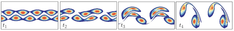
Figure 2: Schematic of the temporally evolving jet. The evolution of the base flow at different time instances ($t_{1}=12$, $t_{2}=15$, $t_{3}=18$, $t_{4}=21$).

3.3.2 Harmonic forcing

To generate the localized forcing, we introduce the following expressions:

$$\tilde{f}_{x}(x,y) =\frac{I(y)}{\beta}\sin(\alpha y)\cos(\beta x),$$ (24)

$$\tilde{f}_{y}(x,y) =-\dfrac{I(y)}{\alpha}\sin(\beta x)\cos(\alpha y),$$ (25)

where $I(y)=\tanh\Big{(}\dfrac{(y-y_{s})}{\delta}\Big{)}-\tanh\Big{(}\dfrac{(y-y_{e})}{\delta}\Big{)}$ serves as the indicator function that localizes the forcing within the region defined by $y_{s}\leq y\leq y_{e}$ and different forcings are generated by varying $\alpha$ and $\beta$. The vector field $(\tilde{f}_{x},\tilde{f}_{y})$ is not divergence-free due to the multiplication of $I(y)$ by each component. We map this vector field to a divergence-free vector field using the projection function $\phi$, which is obtained by solving $\nabla^{2}\phi=\nabla\cdot\tilde{f}$ and updating the vector field using the following relations:

$$f_{x}(x,y,t) =c(\tilde{f}_{x}(x,y)-\frac{\partial\phi}{\partial x})\sin(\omega t),$$ (26)

$$f_{y}(x,y,t) =c(\tilde{f}_{y}(x,y)-\frac{\partial\phi}{\partial y})\sin(\omega t).$$ (27)

It is easy to verify that the vector field $(f_{x},f_{y})$ is divergence-free. Here, the coefficient $c$ determines the energy spectrum of each force component and is given by $c=2\pi/(k_{x}+k_{y})$, where $k_{x}=\alpha/2\pi$ and $k_{y}=\beta/2\pi$. We consider a total of $d=144$ external excitations by varying the wave numbers $k_{x}=[1,2,\dots,12]$ and $k_{y}=[1,2,\dots,12]$. We consider the tensor product of these sets and generate $d=144$ forcings. The temporal forcing frequency is denoted by $\omega$, and for all the forcings considered in this problem, we set $\omega=0.37$. This excitation frequency is identified as one of the dominant frequencies in the nonlinear base flow.

The space-time discretization of the f-OTD equation is identical to that of the FOM. To initialize the f-OTD modes and modal coefficients, we solve the FOM for one time step for all $d=144$ forcings. We construct a matrix of the FOM solution, wherein the matrix has $2N_{x}N_{y}=2^{15}$ rows, corresponding to the total number of grid points times two for the two components of velocity, and $d=144$ columns, with each column representing the response to each forcing. We then perform SVD on this matrix and set the rank-$r$ matrix SVD-truncated matrix as the initial condition for the f-OTD subspace. For very large dynamical systems, the initial condition for the f-OTD matrices can be computed through a targeted sparse sampling of the FOM to reduce computational costs $\big{(}$[39]$\big{)}$.

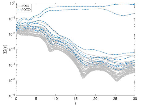
Figure 3: Temporally evolving jet: Comparison of the dominant normalized singular values obtained from FOM and f-OTD.

Figure 3 displays a comparison of normalized singular values between FOM and f-OTD. To compute the normalized singular values, we divide the instantaneous singular value from f-OTD and FOM by the total sum of the FOM singular values at each time instance. We solve the f-OTD equations with a rank of $r=8$, and Figure 3 illustrates that the largest singular values are accurately approximated by f-OTD. The dimensionality of this system varies over time, as observed by the clustering of singular values at the beginning ($0\leq t\leq 5$) where many modes are required to approximate the FOM. As the flow evolves, two time-dependent f-OTD modes become dominant—growing by two to three orders of magnitude larger than the other modes. The dominance of the first two singular values suggests that the response to various forcings can be accurately approximated with a low-rank approximation based on time-dependent bases.

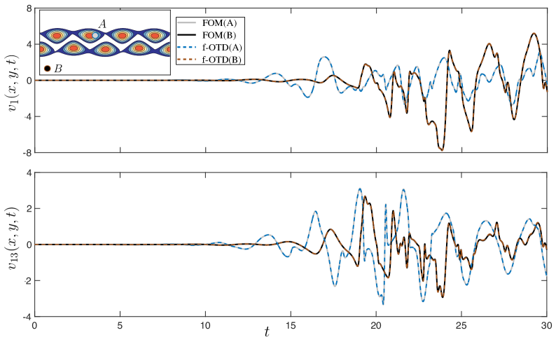
Figure 4: Temporally evolving jet: Comparison of the temporal evolution of the perturbation velocity at two probe locations of $(x_{A},y_{A})=(0.39,0.59)$ and $(x_{B},y_{B})=(0.10,0.12)$.

Figure 4 demonstrates the efficacy of f-OTD reduction in reconstructing the disturbance field when there is a strong cross-frequency interaction between the forcing frequency and the base flow. We examine two distinct excitations, $v_{1}$ and $v_{13}$, corresponding to wavenumbers $(k_{x},k_{y})=(1,1)$ and $(k_{x},k_{y})=(2,1)$, respectively. The figure presents a comparison of the temporal evolution of the f-OTD reconstructed response and the FOM at two different locations, $A$ and $B$, with coordinates $(x_{A},y_{A})=(0.39,0.59)$ and $(x_{B},y_{B})=(0.10,0.12)$. The disturbance exhibits transitional multi-frequency behavior, attributable to the cross-frequency interactions between the harmonic forcing frequency and the arbitrarily time-dependent base flow. It is observed that f-OTD low-rank approximation captures this evolution accurately.

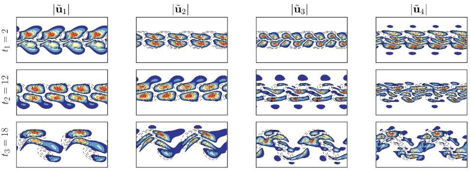
Figure 5: Temporally evolving jet: The first four dominant left singular vectors of the f-OTD low-rank solution operator at different times (dashed line shows the base flow’s vorticity). The f-OTD modes are energetically ranked in descending order.

Figure 5 displays snapshots of the first four dominant f-OTD spatial modes at different time instances, sorted by their singular values from the most dominant to the least dominant modes. The dashed lines show the contours of vorticity for the base flow. The first two modes are associated with the dominant singular values, $\sigma_{1}(t)$ and $\sigma_{2}(t)$, and exhibit similar structures. The dominant modes capture the largest structures, while the lower modes extract finer structures. It is also evident that the f-OTD modes evolve instantaneously with the base flow.

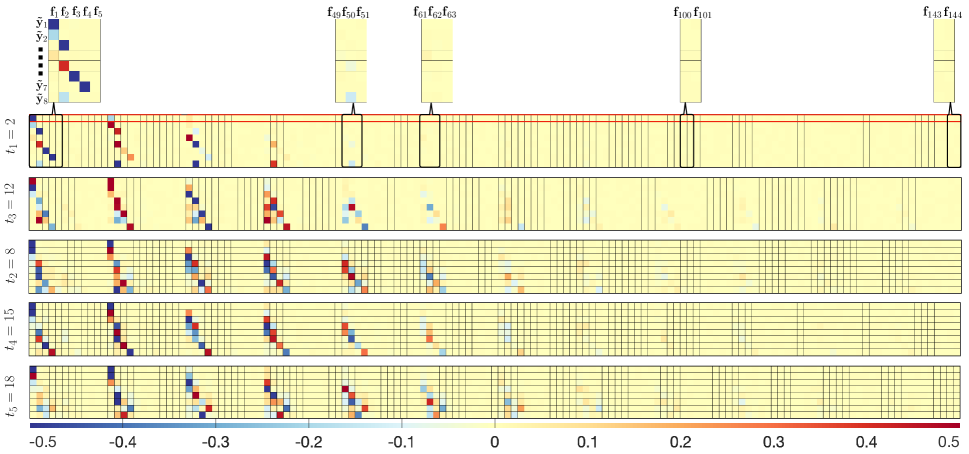
Figure 6: Temporally evolving jet: The first eight dominant right singular vectors ($\mathbf{\tilde{Y}}^{T}(t)$) of the f-OTD low-rank solution operator at different times.

Figure 6 shows the time evolution of the orthonormalized modal coefficients $\mathbf{\tilde{Y}}(t)^{T}$. Each row approximates a right singular vector of the solution operator, while each column represents the contribution of each excitation to different modes. As time progresses, the modal coefficients evolve, capturing the time-dependent contribution of different forces to the f-OTD low-rank subspace. For example, at $t_{1}=2$, the first row ($\mathbf{\tilde{y}}_{1}^{T}$) shows that among all $144$ excitations, $\mathbf{f}_{1}$ and $\mathbf{f}_{13}$, associated with wave numbers $(k_{x},k_{y})=(1,1)$ and $(2,1)$ respectively, have the most significant contributions. However, the third row ($\mathbf{\tilde{y}}_{3}^{T}$), associated with $\sigma_{3}$, demonstrates the dominant contributions of $\mathbf{f}_{2}$ and $\mathbf{f}_{14}$. The modal coefficients contain rich insights into the excitations and can be exploited for physical or dynamical understanding.

We utilize the low-rank approximation of the solution operator based on f-OTD to determine the optimal forcing without incurring additional computational costs. In particular, we seek to identify the forcing $\mathbf{f}\in\mathcal{S}$ whose response achieves maximum amplification at $t=t^{*}$ among all forcings in $\mathcal{S}$. As demonstrated in Section 2.2.3, the optimal forcing is obtained from $\mathbf{f}^{*}=\mathbf{F}\mathbf{\tilde{y}}_{1}(t^{*})$, leading to maximal amplification at the designated time $t^{*}$. To obtain the optimal perturbation vector, we solved Eq. 4 with the forcing $\mathbf{f}=\mathbf{F}\mathbf{\tilde{y}}_{1}(t^{*})$. To underscore the significance of the optimal forcing vector $\mathbf{\tilde{y}}_{1}(t^{*})$, we solved Eq. 4 for a random excitation, $\mathbf{f}_{\text{Rand}}=\mathbf{F}\mathbf{y}_{\text{Rand}}$, where $\|\mathbf{y}_{\text{Rand}}\|$=1. In Panel 7a, we compare the evolution of disturbance energy resulting from these two different external forcings. The gray line represents the maximum possible amplification $G_{\text{max}}(t)=\sigma_{1}^{2}(t)$, which signifies the maximal energy that any $\mathbf{f}\in\mathcal{S}$ can achieve; it can be regarded as the envelope of perturbation energy for all $\mathbf{f}=\mathbf{F}\mathbf{y}$ where $\|\mathbf{y}\|=1$. It is evident that the response to the optimal forcing, shown by the dashed black line, reaches the envelope ($\sigma^{2}_{1}$) at $t^{*}$, shown by a blue circle, after which its energy decays. In contrast, the energy of the random excitation experiences growth but remains roughly one to two orders of magnitude smaller than the maximum possible amplification.

To demonstrate the capability of f-OTD as a rapid surrogate model, we obtain state disturbance due to the optimal forcing using the operator:

$$\mathbf{v}^{*}(t)=\mathbf{H}^{t}_{\mathcal{S}}(\mathbf{\tilde{y}}_{1}(t^{*}))=\tilde{\mathbf{U}}(t)\bm{\Sigma}(t)\tilde{\mathbf{Y}}(t)^{T}(\mathbf{\tilde{y}}_{1}(t^{*})).$$

Note that $\mathbf{\tilde{y}}_{1}(t^{*})$ is not a time-dependent vector. The energy of this solution is shown with cross-marker symbols, which matches well with the disturbance obtained by solving Eq. 4, which is the ground truth in this setting.

Panels 7b-e illustrate the structures of these excitations and their corresponding responses at time $t^{*}$. The x-component of the response to the forcing is shown in panels (7c and 7e). The optimal forcing in Panel 7b exhibits a significant presence in the shear layer and is influenced by lower wave numbers. In panels 7c and 7e we observe that the flow responses share similar structures, however, they have completely different magnitudes. The fact that the disturbance resulting from the random forcing has a shape similar to that of the optimal disturbance is because $\mathbf{y}_{\text{Rand}}$ has a small projection onto the optimal $\mathbf{\tilde{y}}_{1}(t^{*})$. Given that this direction in the forcing space grows significantly faster than other directions, its response ultimately dominates the shape of the disturbance.

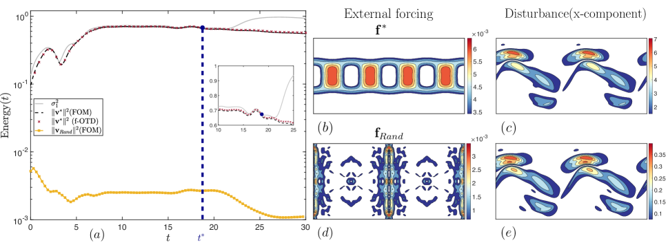
Figure 7: Temporally evolving jet: Comparison between optimal forcing and a random forcing within the forcing space. At time $t^{*}=18.75$, the magnitude of the optimal and random forcing with their corresponding responses are displayed.

l

3.4 Two-dimensional decaying isotropic turbulence

To demonstrate the effectiveness of the f-OTD low-rank approximation, we consider the two-dimensional decaying turbulent flow. This flow is chosen due to its complex dynamics, highly unsteady and time-dependent base flows, and chaotic nature $\big{(}$[46]$\big{)}$. Furthermore, we introduce non-harmonic forcings, which is equivalent to considering forcings composed of a broad spectrum of frequencies. The simulations are conducted using the same numerical methods as those explained in Section 3.3. The computational domain is a square with length $L=2\pi$ and is discretized with a $128\times 128$ grid. The flow fields are initialized using the Taylor-Green vortex $\big{(}$[47]$\big{)}$.

We consider global divergence-free external excitations that are global in space but localized in time. The external forcing is defined as:

$$f_{x}(x,y,t) =\frac{c}{\beta}\sin(\alpha y)\cos(\beta x)g(t),$$ (28)

$$f_{y}(x,y,t) =-\dfrac{c}{\alpha}\sin(\beta x)\cos(\alpha y)g(t).$$ (29)

where $\alpha=\dfrac{2\pi k_{x}}{L}$, $\beta=\dfrac{2\pi k_{y}}{L}$ and $c=\dfrac{1}{(s(k_{x}-1)+k_{y})^{1.35}}$ is the forcing spectrum. Here, $k_{x}$ and $k_{y}$ are the wave numbers ranging from $1$ to $s=10$. The localized temporal function is defined as $g(t)=\exp\left(-(t-t_{0})^{2}/\sigma^{2}\right)$, where $\sigma$ controls the duration of the activation, and $t_{0}$ determines the time of activation. For this study, we set $\sigma$ to 0.8 and $t_{0}$ to 4. The total number of external excitations considered is $d=100$, and using a subspace size of $r=10$ for the f-OTD reduction yields satisfactory results.

Figure LABEL:fig:2D_Turbulent_Error presents a comparison of the reconstruction error between f-OTD ($e(t)$) and the optimal low-rank approximation ($e_{u}(t)$) with a rank of $10$. The error ($e_{u}(t)$) counts as the lower bound for the f-OTD error, representing the minimum error achievable by any rank-$10$ approximation. We calculate the relative error percentage as $\%\text{Error}=\dfrac{e(t)}{\lVert V(t)\rVert_{F}}\times 100$. Over time, we observe that the f-OTD error is larger than the optimal error due to f-OTD losing interactions with unresolved modes. However, the magnitude of the error is of the same order as that of the optimal error. In summary, the maximum error from f-OTD is approximately $\%7.5$, and it gradually decreases over time. Figure LABEL:fig:2D_Turbulent_SVD illustrates the evolution of the first $32$ normalized singular values for both FOM and f-OTD.

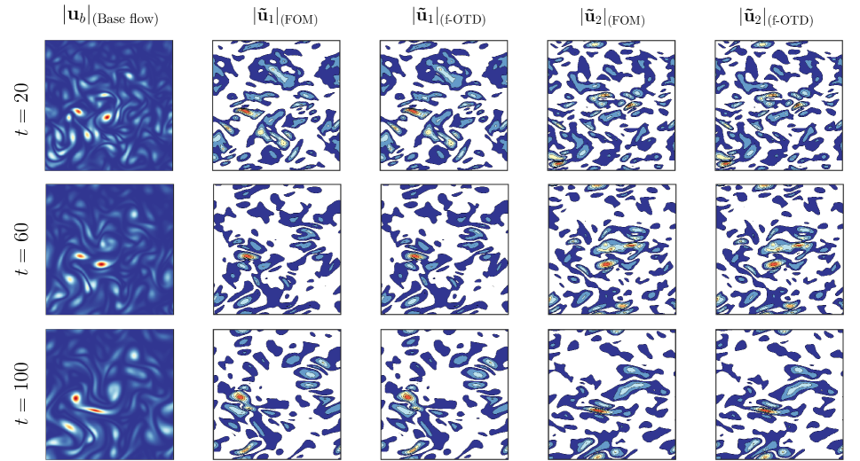
Figure 9: 2D Turbulent flow: Evolution of the first two dominant f-OTD with FOM over time.

Figure 9 shows the time-dependent evolution of the first two dominant f-OTD modes in canonical form. It is readily apparent that the dominant structures extracted by f-OTD are in good agreement with those obtained from the SVD of FOM, which necessitates solving for all $d=100$ samples. Additionally, the modes evolve in concert with the base flow. These results validate the accuracy of f-OTD modes in capturing the most significant structures directly from the dynamical system.

4 Conclusion

Analysis of linear disturbance growth due to external forcing is crucial for flow stability, control, and uncertainty quantification. However, when the base flow is arbitrarily time-dependent, the computational tools effective for analyzing steady-state base flows become either inadequate or too computationally prohibitive to use. To this end, we present a methodology to build low-rank solution operators for the linear evolution of disturbance for problems with unsteady base flows. The solution operator is a time-dependent matrix whose evolution equation is governed by forced linearized dynamics. The formulation is based on the forced optimally time-dependent decomposition (f-OTD), in which the solution operator is approximated by the multiplication of two skinny time-dependent matrices. Using a variational principle, evolution equations for these two matrices are derived. The f-OTD low-rank approximation is equivalent to the dynamical low-rank approximation and similarly constrains the solution of the matrix differential equation to a manifold of low-rank matrices.

We demonstrate the utility of the developed methodology through several case studies. These demonstrations show how the methodology can identify the optimal forcing and employ the operator as an effective surrogate model. We also show the connection between the presented methodology and the resolvent analysis. In particular, we show when applied to the steady-state mean flow, the presented low-rank approximation asymptotically converges to that of the resolvent analysis.

Two mathematical developments are of interest for future studies: (i) rigorously proving the connection between the asymptotic behavior of f-OTD and resolvent analysis; (ii) developing a rank-adaptive f-OTD methodology that determines the rank of the low-rank approximation at each time instant, based on the accuracy requirements of the solution operator. accuracy requirements of the solution operator.

Appendix A f-OTD derivation for incompressible Navier–Stokes

In this section, we present the f-OTD evolution equations for the incompressible Navier-Stokes equations. The incompressible Navier-Stokes equations govern the evolution of the base flow as shown below:

$$\frac{\partial{U_{b}}}{\partial t}+({U_{b}}\cdot){\nabla U_{b}} =-{\nabla p}_{b}+\frac{1}{Re}\nabla^{2}{U_{b}},$$ (30)

$${\nabla}\cdot{U_{b}} =0,$$ (31)

where ${U_{b}}(x,y,t)$ is the velocity vector field with components ${U_{b}}(x,y,t)=(u_{b}(x,y,t),v_{b}(x,y,t))$, and ${p}_{b}(x,y,t)$ is the pressure field. The evolution equation for disturbance $v_{i}(x,y,t)$ is given by

$$\frac{\partial v_{i}}{\partial t} =\mathcal{L}_{NS}(v_{i})-\nabla p_{i}+f_{i}$$ (32)

$${\nabla}\cdot{v_{i}} =0,$$ (33)

where $\mathcal{L}_{NS}(\sim)$ is the linearized Navier-Stokes operator given by

$$\mathcal{L}_{NS}(v_{i})=-(U_{b}\cdot\nabla)v_{i}-(v_{i}\cdot\nabla)U_{b}+\frac{1}{Re}\nabla^{2}v_{i},\quad i=1,2,\dots,d$$ (34)

and $f_{i}(x,y,t)$ is the external forcing. The matrix $\mathbf{L}$ and vector $\mathbf{f}_{i}$ in the f-OTD evolution equations are the discrete representation of $\mathcal{L}_{NS}$ and $f_{i}(x,y,t)$, respectively. For incompressible Navier-Stokes equation, each f-OTD mode is a vector field, that is, $u_{i}=(u_{x_{i}},u_{y_{i}})$, for $i=1,\ldots,r$. The f-OTD modes are orthonormal with respect to the following inner product:

$$\big{<}u_{i},u_{j}\big{>}=\int\int(u_{x_{i}}u_{x_{j}}+u_{y_{i}}u_{y_{j}})\,dx\,dy,\quad\quad\|u\|=\big{<}u,u\big{>}^{1/2}.$$

The induced norm is also defined above. Moreover, the f-OTD vector field must be divergence-free to ensure that any f-OTD reconstructed field is also divergence-free. Therefore, $\nabla\cdot u_{i}=0$. To enforce the divergence-free condition, we use the projection method. Below, we explain the steps for the time integration for the f-OTD equations for an explicit Euler scheme:

1. Solve Eq. 15, in which $\mathbf{L}$ is the discrete representation of $\mathcal{L}_{NS}$ operator given by Eq. 34.

   $$\hat{\mathbf{U}}^{k+1}=\mathbf{U}^{k}+\Delta t\big{(}\mathbf{L}^{k}\mathbf{U}^{k}-\mathbf{U}^{k}\mathbf{L}^{k}_{r}+\big{(}\mathbf{F}^{k}\mathbf{Y}^{k}-\mathbf{U}^{k}\mathbf{U}^{k^{T}}\mathbf{F}^{k}\mathbf{Y}^{k}\big{)}{\mathbf{C}}^{k^{-1}}\big{)},$$ (35)

   where the solution at time step $k$ is denoted with a superscript $(\sim)^{k}$ and $\Delta t$ is the time advancement magnitude. For an efficient implementation of the above step, it is important to note that the matrix $\mathbf{L}$ does not need to be explicitly formed; rather, what is required is the action of $\mathbf{L}$ on vector fields.

2. Note that the pressure gradient is not included in the linearized operator, and as a result, the columns of $\hat{\mathbf{U}}^{k+1}$, denoted by $\hat{\mathbf{u}_{i}}^{k+1}$, are not divergence-free. In this step, we use the projection method to project $\hat{\mathbf{u}_{i}}^{k+1}$ onto a divergence-free vector field:

   $$\mathbf{D}\mathbf{G}\bm{\phi}^{k+1}_{i} =\mathbf{D}\hat{\mathbf{u}_{i}}^{k+1},\quad i=1,2,\dots,r,$$

   $$\mathbf{u}_{i}^{k+1} =\hat{\mathbf{u}_{i}}^{k+1}-\mathbf{G}\bm{\phi}^{k+1}_{i}$$

   where $\mathbf{D}\in\mathbb{R}^{n\times 2n}$ and $\mathbf{G}\in\mathbb{R}^{2n\times n}$ are the discrete representations of the gradient and divergence operators, respectively.

3. In the last step, we advance the evolution equation for the f-OTD coefficients using the divergence-free f-OTD modes: $\mathbf{U}^{k+1}=[\mathbf{u}_{1}^{k+1},\mathbf{u}_{2}^{k+1},\dots,\mathbf{u}_{r}^{k+1}]$.

   $$\mathbf{Y}^{k+1}=\mathbf{Y}^{k}+\Delta t\big{(}\mathbf{Y}^{k}\mathbf{L}_{r}^{k^{T}}+\mathbf{F}^{k^{T}}\mathbf{U}^{k}\big{)}.$$ (36)

We use the fourth-order Runge-Kutta scheme for the time integration of the f-OTD equations. Time advancement of every stage of the Runge-Kutta scheme is analogous to the explicit Euler explained above.

References

- [1] Brian F Farrell. Optimal excitation of baroclinic waves. Journal of Atmospheric Sciences, 46(9):1193–1206, 1989.
- [2] Paolo Luchini and Alessandro Bottaro. Adjoint equations in stability analysis. Annual Review of fluid mechanics, 46:493–517, 2014.
- [3] Pedram Hassanzadeh and Zhiming Kuang. The linear response function of an idealized atmosphere. part i: Construction using green’s functions and applications. Journal of the Atmospheric Sciences, 73(9):3423–3439, 2016.
- [4] Wei Ran, Armin Zare, MJ Philipp Hack, and Mihailo R Jovanović. Stochastic receptivity analysis of boundary layer flow. Physical Review Fluids, 4(9):093901, 2019.
- [5] M Matsubara and P Henrik Alfredsson. Disturbance growth in boundary layers subjected to free-stream turbulence. Journal of fluid mechanics, 430:149–168, 2001.
- [6] Jens HM Fransson, Masaharu Matsubara, and P Henrik Alfredsson. Transition induced by free-stream turbulence. Journal of Fluid Mechanics, 527:1–25, 2005.
- [7] Pierre Ricco, Edmond J Walsh, Flavio Brighenti, and Donald M McEligot. Growth of boundary-layer streaks due to free-stream turbulence. International Journal of Heat and Fluid Flow, 61:272–283, 2016.
- [8] RG Jacobs and PA Durbin. Simulations of bypass transition. Journal of Fluid Mechanics, 428:185–212, 2001.
- [9] Luca Brandt, Philipp Schlatter, and Dan S Henningson. Transition in boundary layers subject to free-stream turbulence. Journal of Fluid Mechanics, 517:167–198, 2004.
- [10] ME Goldstein. Effect of free-stream turbulence on boundary layer transition. Philosophical Transactions of the Royal Society A: Mathematical, Physical and Engineering Sciences, 372(2020):20130354, 2014.
- [11] Beverley J McKeon and Ati S Sharma. A critical-layer framework for turbulent pipe flow. Journal of Fluid Mechanics, 658:336–382, 2010.
- [12] Lloyd N Trefethen, Anne E Trefethen, Satish C Reddy, and Tobin A Driscoll. Hydrodynamic stability without eigenvalues. Science, 261(5121):578–584, 1993.
- [13] Mihailo R Jovanović and Bassam Bamieh. Componentwise energy amplification in channel flows. Journal of Fluid Mechanics, 534:145–183, 2005.
- [14] F Gómez, HM Blackburn, Murray Rudman, AS Sharma, and BJ35103181422 McKeon. A reduced-order model of three-dimensional unsteady flow in a cavity based on the resolvent operator. Journal of Fluid Mechanics, 798, 2016.
- [15] Sean Symon, Denis Sipp, Peter J Schmid, and Beverley J McKeon. Mean and unsteady flow reconstruction using data-assimilation and resolvent analysis. AIAA Journal, 58(2):575–588, 2020.
- [16] Benjamin Herrmann, Peter J Baddoo, Richard Semaan, Steven L Brunton, and Beverley J McKeon. Data-driven resolvent analysis. Journal of Fluid Mechanics, 918, 2021.
- [17] Shervin Bagheri, Luca Brandt, and Dan S Henningson. Input–output analysis, model reduction and control of the flat-plate boundary layer. Journal of Fluid Mechanics, 620:263–298, 2009.
- [18] R Moarref, MR Jovanović, JA Tropp, AS Sharma, and BJ McKeon. A low-order decomposition of turbulent channel flow via resolvent analysis and convex optimization. Physics of Fluids, 26(5):051701, 2014.
- [19] Ethan Pickering, Georgios Rigas, Oliver T Schmidt, Denis Sipp, and Tim Colonius. Optimal eddy viscosity for resolvent-based models of coherent structures in turbulent jets. Journal of Fluid Mechanics, 917:A29, 2021.
- [20] Alberto Padovan, Samuel E Otto, and Clarence W Rowley. Analysis of amplification mechanisms and cross-frequency interactions in nonlinear flows via the harmonic resolvent. Journal of Fluid Mechanics, 900, 2020.
- [21] Alberto Padovan and Clarence W Rowley. Analysis of the dynamics of subharmonic flow structures via the harmonic resolvent: Application to vortex pairing in an axisymmetric jet. Physical Review Fluids, 7(7):073903, 2022.
- [22] Michael Donello, Mark H Carpenter, and Hessam Babaee. Computing sensitivities in evolutionary systems: a real-time reduced order modeling strategy. SIAM Journal on Scientific Computing, 44(1):A128–A149, 2022.
- [23] H Babaee and TP Sapsis. A minimization principle for the description of modes associated with finite-time instabilities. Proceedings of the Royal Society A: Mathematical, Physical and Engineering Sciences, 472(2186):20150779, 2016.
- [24] Hessam Babaee, Mohamad Farazmand, George Haller, and Themistoklis P Sapsis. Reduced-order description of transient instabilities and computation of finite-time lyapunov exponents. Chaos: An Interdisciplinary Journal of Nonlinear Science, 27(6):063103, 2017.
- [25] Miguel Beneitez, Yohann Duguet, Philipp Schlatter, and Dan S Henningson. Edge manifold as a lagrangian coherent structure in a high-dimensional state space. Physical Review Research, 2(3):033258, 2020.
- [26] Mohammad Farazmand and Themistoklis P Sapsis. Dynamical indicators for the prediction of bursting phenomena in high-dimensional systems. Physical Review E, 94(3):032212, 2016.
- [27] Antoine Blanchard and Themistoklis P Sapsis. Stabilization of unsteady flows by reduced-order control with optimally time-dependent modes. Physical Review Fluids, 4(5):053902, 2019.
- [28] J Simon Kern, Miguel Beneitez, Ardeshir Hanifi, and Dan S Henningson. Transient linear stability of pulsating poiseuille flow using optimally time-dependent modes. Journal of Fluid Mechanics, 927, 2021.
- [29] Yonghong Zhong, Alireza Amiri-Margavi, Hessam Babaee, and Kunihiko Taira. Optimally time-dependent mode analysis of vortex gust-airfoil wake interactions. Bulletin of the American Physical Society, 2022.
- [30] Yinmin Liu, Hessam Babaee, Peyman Givi, Harsha K. Chelliah, Daniel Livescu, and Arash G. Nouri. Skeletal reaction models for methane combustion. Fuel, 357:129581, 2024.
- [31] AG Nouri, H Babaee, P Givi, HK Chelliah, and Daniel Livescu. Skeletal model reduction with forced optimally time dependent modes. Combustion and Flame, 235:111684, 2022.
- [32] M. H. Beck, A. Jäckle, G. A. Worth, and H. D. Meyer. The multiconfiguration time-dependent Hartree (MCTDH) method: a highly efficient algorithm for propagating wavepackets. Physics Reports, 324(1):1–105, 1 2000.
- [33] O. Koch and C. Lubich. Dynamical low-rank approximation. SIAM Journal on Matrix Analysis and Applications, 29(2):434–454, 2017/04/02 2007.
- [34] T.P. Sapsis and P.F.J. Lermusiaux. Dynamically orthogonal field equations for continuous stochastic dynamical systems. Physica D: Nonlinear Phenomena, 238(23-24):2347–2360, 2009.
- [35] P. Patil and H. Babaee. Real-time reduced-order modeling of stochastic partial differential equations via time-dependent subspaces. Journal of Computational Physics, 415:109511, 2020.
- [36] D. Ramezanian, A. G. Nouri, and H. Babaee. On-the-fly reduced order modeling of passive and reactive species via time-dependent manifolds. Computer Methods in Applied Mechanics and Engineering, 382:113882, 2021.
- [37] L. Einkemmer and C. Lubich. A low-rank projector-splitting integrator for the vlasov–poisson equation. SIAM Journal on Scientific Computing, 40(5):B1330–B1360, 2023/08/15 2018.
- [38] Kusch, J. and Stammer, P. A robust collision source method for rank adaptive dynamical low-rank approximation in radiation therapy. ESAIM: M2AN, 57(2):865–891, 2023.
- [39] M. Donello, G. Palkar, M. H. Naderi, D. C. Del Rey Fernández, and H. Babaee. Oblique projection for scalable rank-adaptive reduced-order modelling of nonlinear stochastic partial differential equations with time-dependent bases. Proceedings of the Royal Society A: Mathematical, Physical and Engineering Sciences, 479(2278):20230320, 2023/10/19 2023.
- [40] P. J. Schmid. Nonmodal stability theory. Annu. Rev. Fluid Mech., 39:129–162, 2007.
- [41] M. H. Naderi and H. Babaee. Adaptive sparse interpolation for accelerating nonlinear stochastic reduced-order modeling with time-dependent bases. Computer Methods in Applied Mechanics and Engineering, 405:115813, 2023.
- [42] B.R. Noack, K. Afanasiev, M. Morzynski, G. Tadmor, and F. Thiele. A hierarchy of low-dimensional models for the transient and post-transient cylinder wake. Journal of Fluid Mechanics, 497(-1):335–363, 2003.
- [43] Aly-Khan Kassam and Lloyd N Trefethen. Fourth-order time-stepping for stiff pdes. SIAM Journal on Scientific Computing, 26(4):1214–1233, 2005.
- [44] George Broze and Fazle Hussain. Nonlinear dynamics of forced transitional jets: temporal attractors and transitions to chaos. In Nonlinear Instability of Nonparallel Flows, pages 459–473. Springer, 1994.
- [45] Cristobal Arratia, CP Caulfield, and J-M Chomaz. Transient perturbation growth in time-dependent mixing layers. Journal of Fluid Mechanics, 717:90–133, 2013.
- [46] Javier Jiménez. Monte carlo science. Journal of Turbulence, 21(9-10):544–566, 2020.
- [47] Ville Vuorinen and K Keskinen. Dnslab: A gateway to turbulent flow simulation in matlab. Computer Physics Communications, 203:278–289, 2016.