XMM-Newton - NuSTAR monitoring campaign of the Seyfert 1 galaxy IC 4329A

We present the results of a joint XMM-Newton and NuSTAR campaign on the active galactic nucleus (AGN) IC 4329A, consisting of 9 $\times$ 20 ks XMM-Newton observations, and 5 $\times$ 20 ks NuSTAR observations within nine days, performed in August 2021. Within each observation, the AGN is not very variable, with the fractional variability never exceeding 5%. Flux variations are observed between the different observations, on timescales of days, with a 30% ratio between the minimum and the maximum 2–10 keV flux. These variations follow the softer-when-brighter behavior typically observed in AGN. In all observations, a soft excess is clearly present. Consistently with previous observations, the X-ray spectra of the source exhibit a cut-off energy between 140 and 250 keV, constant within the error in the different observations. We detected a narrow iron K$\alpha$ line consistent with being constant during the monitoring, and likely originating in a distant neutral medium. We do not find evidence of a broad component of the iron line, suggesting that the inner disk does not produce strong reflection. We find that the reflection component is weak ($R_{\rm max}=0.009\pm 0.002$). We also found the presence of a warm absorber component together with an ultra-fast outflow. Looking at their energetic, these outflows have enough mechanical power to exercise a significant feedback impact on the AGN surrounding environment.

1 Introduction

Active Galactic Nuclei (AGN) are extremely luminous, compact objects located at the center of massive galaxies. They are powered by accretion of gas onto the central supermassive black hole (SMBH, $M_{\rm BH}>10^{5}$ $M_{\odot}$; Salpeter 1964; Ho 2008). The X-ray emission of AGN is due to high-energy processes occurring in the so-called hot corona, which contains high-energy electrons and is located near the SMBH (Haardt & Maraschi 1991; Haardt et al. 1994, 1997; Merloni 2003; Fabian et al. 2009; Zoghbi et al. 2012; De Marco et al. 2013). The hot electrons interact with thermal UV/optical photons emitted by the accretion disc through inverse-Compton scattering, which boosts the energy of the photons into the X-ray band. This process produces a broad power law continuum in the X-ray spectrum with a cutoff at high energy (e.g., Sunyaev & Titarchuk 1980; Haardt & Maraschi 1993). Cold circumnuclear materials, such as the optically thick accretion disc and/or the molecular torus, absorb and reprocess the X-rays, which results in a feature in the X-ray spectrum known as Compton reflection, which peaks at around $\sim 30$ keV (Pounds et al. 1990; George & Fabian 1991). Additionally, the reflection process produces absorption and emission lines, such as the prominent FeK$\alpha$ emission line at 6.4 keV (Nandra & Pounds 1994), which are the result of photoelectric absorption and fluorescence (Matt et al. 1997).

IC 4329A is a bright nearby (z=0.01598, Koss et al. 2022) AGN and it is classified in the optical as a Seyfert 1.5 galaxy (Oh et al. 2022). It is located at the center of an edge-on host galaxy, with a dust lane passing through the nucleus. It shows also a dusty lukewarm absorber in the UV band (i.e. $T\sim 3\times 10^{4}$ K, Crenshaw & Kraemer 2001), characterized by saturated UV absorption lines (C IV, N V) near the systemic velocity of the host galaxy, likely responsible for reddening both the continuum and the emission lines. The black hole mass of IC 4329A is $M_{\rm BH}=6.8^{+1.2}_{-1.1}\times 10^{7}M_{\odot}$ (Bentz et al. 2023) and its Eddington ratio is $\lambda_{\rm Edd}=L_{\rm bol}/L_{\rm Edd}=0.17$. This was computed using the bolometric luminosities calculated from the intrinsic luminosities in the 14–150 keV range, as shown in Ricci et al. 2017, with a bolometric correction of 8 (Koss et al. 2022).

IC 4329A has been extensively studied in the X-ray band in the last decades by all major X-rays satellites including Einstein (Petre et al. 1984; Holt et al. 1989), EXOSAT (Singh et al. 1991), Ginga (Piro et al. 1990), ASCA/RXTE (Done et al. 2000), BeppoSAX (Perola et al. 2002; Dadina 2007), Chandra (McKernan & Yaqoob 2004; Shu et al. 2010a), XMM-Newton (Steenbrugge et al. 2005; Nandra et al. 2007; Mehdipour & Costantini 2018), INTEGRAL (Beckmann et al. 2006), Swift/BAT (Winter et al. 2009; Ricci et al. 2017), Suzaku (Mantovani et al. 2014) NuSTAR (Brenneman et al. 2014a, b), AstroSat (Tripathi et al. 2021; Dewangan et al. 2021). It has a 2–10 keV flux that ranges between $8.1\times 10^{-11}$ $\rm erg\,\rm cm^{-2}\,\rm s^{-1}$ (Winter et al. 2009) and $1.8\times 10^{-9}$ $\rm erg\,\rm cm^{-2}\,\rm s^{-1}$ (Shu et al. 2010a). The past BeppoSax, ASCA+RXTE INTEGRAL and Swift/BAT observations of IC 4329A placed a rough constraints on the high-energy cut-off respectively at $E_{\rm c}\geq 180$ keV (Perola et al. 2002), $E_{\rm c}=150-390$ keV (Done et al. 2000), $E_{\rm c}=60-300$ keV (Molina et al. 2013) and $E_{\rm c}>190$ keV (Ricci et al. 2017). The NuSTAR hard X-ray spectrum of this AGN is characterized by a power law with a photon-index of $\Gamma=1.73\pm 0.01$ and a high-energy cut-off at $E_{\rm c}=186\pm 14$ keV (Brenneman et al. 2014b). Past analysis showed also the presence of a neutral reflection component with a reflection fraction of $R_{\rm refl}=0.42\pm 0.02$ (Mantovani et al. 2014).

This source is well known to exhibit the presence of a strong Fe K$\alpha$ line (Piro et al. 1990). The Fe K$\alpha$ line in IC 4329A shows a narrow core at $6.4$ keV consistent with being produced by low-ionization material either in the outer accretion disc, in the broad line region, or in the torus. The narrow core component of the Fe K$\alpha$ shows also variability on timescales of weeks to months (Fukazawa et al. 2016; Andonie et al. 2022). From the analysis of the ASCA, RXTE, BeppoSAX, Suzaku and NuSTAR observations (Done et al. 2000; Dadina 2007; Brenneman et al. 2014b; Mantovani et al. 2014) the presence of a broad component was reported, most likely produced in the inner part of the accretion disc, and blurred by general relativistic effects. In other works (e.g. McKernan & Yaqoob 2004; Markowitz et al. 2006; Nandra et al. 2007; Tripathi et al. 2021) the observations suggest a modest or weak broad iron line indicating that X–ray reflection from the inner disk is weak in this source. Analysing the Suzaku and NuSTAR observations of IC 4329A with a relativistic reflection model, Ogawa et al. (2019) inferred a very low reflection fraction ($R\sim 3.2\times 10^{-3}$).

IC 4329A also shows the presence of an ionized warm absorber component with $\log(\xi/\rm erg\,\rm s^{-1}\,\rm cm)$ in the range of $-1.37$ and $2.7$ (Steenbrugge et al. 2005) and also a highly ionised, i.e. $\log(\xi/\rm erg\,\rm s^{-1}\,\rm cm)$ $=5.34\pm 0.94$, ultra fast outflowing component (UFO, Tombesi et al. 2015), with outflow velocity $v/c=0.098\pm 0.004$. The presence of this component was first detected by Markowitz et al. (2006) and then confirmed by Tombesi et al. (2011).

Recently IC 4329A has been observed by the Imaging X-ray Polarimetry Explorer (IXPE) for $\sim 500$ ks. From these observations it appears that the source shows a $1\sigma$ confidence limit on polarization degree of $3.3\%\pm 1.1\%$ and a polarisation angle of $78^{\circ}\pm 10^{\circ}$, consistent with being aligned with the radio jet (Ingram et al. 2023; Pal et al. 2023). These finding favour coronal geometries which are more asymmetric and possibly outflowing. However the coronal geometry is unconstrained within $3\sigma$ confidence level.

Here we present the results of the analysis of the X-ray broad-band spectra from the simultaneous XMM-Newton and NuSTAR observations of IC 4329A. These observations are part of a joint millimeter/X-ray study of this nearby source, which also includes observations from Swift (10 observations), NICER (20 observations) and from the Atacama Large Millimeter/submillimeter Array (ALMA, 10 observations). The aim of the campaign is to study the relation between the 100 GHz and X-ray continuum in AGN, and to test the idea that the mm continuum is associated to self-absorbed synchrotron emission from the X-ray corona (e.g., Laor & Behar 2008; Inoue & Doi 2014), as suggested by the recent discovery of a tight correlation between the X-ray luminosity and the 100 GHz (Ricci et al. 2023) and 200 GHz (Kawamuro et al. 2022) luminosities of nearby AGN. Since this paper is focused on the high-resolution X-ray spectroscopy of IC 4329A, we will not include Swift and NICER data, which will be presented, together with the results of ALMA campaign in a dedicated forthcoming paper (Shablovinskaya et al., in prep).

The paper is organized as follows: in Sect. 2, we present the dataset analysed in this work; in Sect. 3 and Sect. 4 we describe the timing and spectral data analysis processes respectively; in Sect. 5 we discuss the results of our analysis which are summarized in Sect. 6. Standard cosmological parameters (H=70 km s${}^{-1}\rm Mpc^{-1}$, $\Omega_{\Lambda}$=0.73 and $\Omega_{m}$=0.27) are adopted.

2 Data and Data Reduction

Table 1: Summary of the 2021 XMM-Newton and NuSTAR observations of IC 4329A.

Telescope	Obs. ID	Start Date	Exp.
		yyyy-mm-dd	ks
XMM-Newton	0862090101	2021-08-10	22.2
NuSTAR	60702050002	2021-08-10	20.6
XMM-Newton	0862090201	2021-08-11	17
XMM-Newton	0862090301	2021-08-12	24
NuSTAR	60702050004	2021-08-12	21.1
XMM-Newton	0862090401	2021-08-13	20
XMM-Newton	0862090501	2021-08-14	22.5
NuSTAR	60702050006	2021-08-14	19.8
XMM-Newton	0862090601	2021-08-15	17.9
XMM-Newton	0862090701	2021-08-16	23
NuSTAR	60702050008	2021-08-16	18.7
XMM-Newton	0862090801	2021-08-17	19.5
XMM-Newton	0862090901	2021-08-18	21.3
NuSTAR	60702050010	2021-08-18	18
XMM-Newton	0862091001	2021-08-19	21.3

The dataset analysed in this work consists of nine X-ray Multi-Mirror Mission (XMM-Newton, Jansen et al. 2001) observations five of which have been performed simultaneously with the Nuclear Spectroscopic Telescope Array (NuSTAR, Harrison et al. 2013). Details on the duration and exposure of the observations are reported in Table 1.

2.1 XMM-Newton data reduction

IC 4329A has been observed once per day for ten consecutive days (from 2021-08-10 to 2021-08-19) by XMM-Newton (P.I. C. Ricci) during the XMM-Newton AO 19. The XMM-Newton observations have been performed with the European Photon Imaging Camera (EPIC hereafter) detectors, and with the Reflection Grating Spectrometer (RGS hereafter; den Herder et al. 2001). The EPIC cameras were operated in small window and thin filter mode. The observation n. 0862090401 is not included in the analysis since, due to a problem in the ground segment, the EPIC-pn exposure was lost.

The EPIC-pn camera (Strüder et al. 2001) event lists are extracted with the epproc and emproc tools of the standard System Analysis Software (SAS v.18.0.0; Gabriel et al. 2004). The MOS detectors (Turner et al. 2001) and the RGS were not considered because, due to the lower statistics of their spectra, they do not add information to the analysis.

The choice of the optimal time cuts for flaring particle background and of the source and background extraction radii were performed via an iterative process which maximizes the signal-to-noise ratio (SNR) as in Piconcelli et al. (2004). The resulting optimal extraction radius was $30\arcsec$ and the background spectra were extracted from source-free circular regions with radii of $\sim$ $50\arcsec$ for the EPIC-pn for each observations. Response matrices and auxiliary response files were generated using the SAS tools rmfgen and arfgen, respectively. EPIC-pn spectra were binned in order to over-sample the instrumental energy resolution by a factor larger than three and to have no less than 20 counts in each background-subtracted spectral channel. No significant pile-up affected the EPIC data, as indicated by the SAS task epatplot. EPIC-pn light curves were extracted by using the same circular regions for the source and the background as the spectra.

2.2 NuSTAR data reduction

The five NuSTAR observations have been performed, simultaneously with five XMM-Newton observations, during NuSTAR AO 7 (P.I. C. Ricci). NuSTAR telescope observed the source with its two coaligned X-ray telescopes Focal Plane Modules A and B (FPMA and FPMB, respectively).

The NuSTAR high-level products were obtained using the NuSTAR Data Analysis Software (NuSTARDAS) package (v2.1.1) within the heasoft package (version 6.29). Cleaned event files (level 2 data products) were produced and calibrated using standard filtering criteria with the nupipeline task, and the latest calibration files available in the NuSTAR calibration database (CALDB 20220802). For both FPMA and FPMB the radii of the circular region used to extract source and background spectra were both $75\arcsec$; no other bright X-ray source is present within $75\arcsec$ from IC 4329A, and no source was present in the background region. The low-energy (0.2–5 keV) effective area issue for FPMA (Madsen et al. 2020) does not affect our observations, since no low-energy excess is found in the spectrum of this detector. The spectra were binned in order to over-sample the instrumental resolution by at least a factor of 2.5 and to have a SNR greater than 3 in each spectral channel. Light curves are extracted using the nuproducts task, adopting the same circular regions as the spectra.

3 Timing analysis

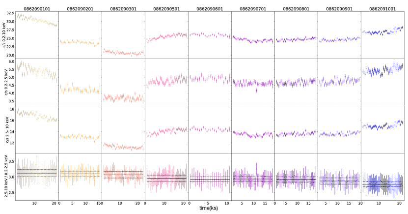
Figure 1: XMM-Newton EPIC-pn light curves (background subtracted) in the 0.2–10 keV, 0.2–2.5 keV and in the 2.5–10 keV are shown in the top, top-middle and bottom-middle panels, respectively. In the bottom panels, the ratios between the XMM-Newton EPIC-pn background subtracted light curves in the 2.5–10 keV and 0.2–2.5 keV energy bands are reported. All the light curves are extracted using a binning time of 500 s. Black solid and dashed lines indicate the average and the standard error of the mean, respectively.

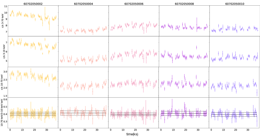
Figure 2: NuSTAR FPMA+B background subtracted light curve in the 3–70 keV. 3–10 keV and 10–70 keV energy ranges are shown in the top, top-middle and bottom-middle panels, respectively. In the bottom panels the ratios between the NuSTAR NuSTAR background subtracted light curves in the 10–70 keV and 3–10 keV energy bands are reported. All the light curves are extracted using a binning time of 500 s. Black solid and dashed lines indicate the average and the standard error of the mean respectively.

During the monitoring, IC 4329A varied within some observations. However, these variations do not affect the ratio between the flux in the 2.5–10 keV and the 0.2–2.5 keV band, (¡ 15%, see bottom panels of Fig. 1).

We looked at the variability spectra of the XMM-Newton EPIC-pn observations of IC 4329A using one of the common estimators for X-ray variability: the fractional variability F_var (Vaughan et al. 2004; Papadakis 2004; McHardy et al. 2006; Ponti et al. 2012; Matzeu et al. 2016, 2017; De Marco et al. 2020). The F_var, i.e. the square root of the normalized excess variance ($\sigma^{2}_{\rm NXS}$ Nandra et al. 1997a; Edelson et al. 2002; Vaughan et al. 2003), is the difference between the total variance of the light curve and the mean squared error that is normalised for the average of the number of flux measurements squared. Being N the number of good time intervals in a light curve, and $x_{i}$ and $\sigma_{i}$ respectively the flux and the error in each interval, F_var is defined (Vaughan et al. 2003) as:

$$F_{\rm var}=\sqrt{\sigma^{2}_{\rm NXS}}=\sqrt{\frac{S^{2}-\overline{\sigma^{2}}}{\overline{x_{i}}^{2}}}$$ (1)

Where: $S^{2}=\frac{1}{N-1}\sum_{i=1}^{N}[(x_{i}-\overline{x_{i}})^{2}]$ is the sample variance, i.e. the integral of the power spectral density (PDS) between two frequencies, and $\overline{\sigma^{2}}=\frac{1}{N}\sum_{i=1}^{N}[\sigma_{i}^{2}]$ is the mean square error.

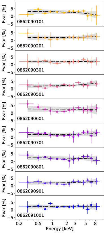
Figure 3: Fractional variability spectra for the XMM-Newton EPIC-pn observations of IC 4329A as in Table 1. The spectra of this campaign are characterised by a mostly flat shape, with the fractional variability which never exceeds the 5%. The dotted dashed black lines are the linear regressions while the shaded regions represent the combined 3$\sigma$ error on the slope and normalisation.

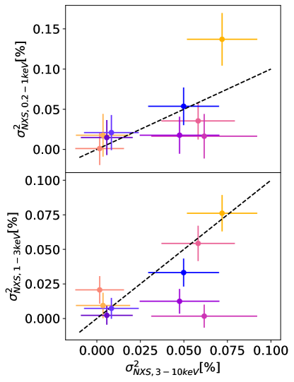
Figure 4: Top panel: soft (0.2–1 keV) vs hard (3–10 keV) $\sigma_{\rm NXS}^{2}$. Bottom panel: medium(1–3 keV) vs hard (3–10 keV) $\sigma_{\rm NXS}^{2}$. The values are calculated for the XMM-Newton EPIC-pn observations of IC 4329A as in Table 1. The black dashed lines represent the one-to-one relation. The color code for different observations is the same as in Fig. 3.

We computed F_var for each observation using the background-subtracted EPIC-pn light curves in different energy bands using a temporal bin of 1000 s on a timescale of 20 ks. The errors are computed using Eq. B2 of Vaughan et al. (2003). The resulting F_var spectra of each observation are shown in Fig. 3. To study the behaviour of the variability spectra, we used the linmix code, a hierarchical Bayesian model for fitting a straight line to data with errors in both the x and y directions (Kelly 2007). To perform the fitting we used a linear model of the data using the following fitting relation:

$$F_{\rm var}=\alpha\times E+\beta$$ (2)

We found the behaviour of the variability spectra of this campaign to be nearly flat, with a correlation coefficient $\rho_{\rm Pearson}$ spanning between -0.05 and 0.05.

The different spectral component observed in AGN can lead to spectral variability in different energy bands as each of them can dominate in a certain energy band. For example the primary power law component or the reflection component are dominant in the hard energy band (3–10 keV, Haardt & Maraschi 1991, 1993; Haardt & Matt 1993) while soft-excess and warm-absorbers (WA) can dominate the soft (0.2–1 keV, Bianchi et al. 2009) and medium (1–3 keV, Blustin et al. 2005; Tombesi et al. 2013) energy bands. We therefore calculated the $\sigma_{\rm NXS}^{2}$ from the 0.2–1 keV (soft), 1–3 keV (medium) and 3–10 keV (hard) light curves, to get a complete picture of the X-ray variability of IC 4329A, and we compared these values in Fig. 4. The $\sigma_{\rm NXS}^{2}$ in the soft, medium and hard energy band for the XMM-Newton observations of IC 4329A in this campaign, in general, are very low. They are below 0.1% in all the observations except for the $\sigma^{2}_{\rm NXS}$ in the soft energy band of the Obs.ID 0862090101 (0.15%). Looking at the $\sigma^{2}_{\rm NXS,1-3\,keV}$ vs $\sigma^{2}_{\rm NXS,3-10\,keV}$ values, they are located in the vicinity or slightly below the one-to-one relation. The same is for the $\sigma^{2}_{\rm NXS,0.2-1\,keV}$ vs $\sigma^{2}_{\rm NXS,3-10\,keV}$ values except again for Obs.ID 0862090101 which is located above the one-to-one relation. This could also be related to the small peak of the variability spectrum of this observation at around 0.5 keV. Thus, overall IC 4329A shows very weak variations. Our analysis shows that the soft-excess and/or warm absorber components variations are weaker than those of the primary continuum and/or reflection component on the timescale of 20 ks except for the Obs.ID 0862090101 in which most likely the soft-excess or the absorbing components are more variable on timescales less than $\sim 20$ ks with respect to the continuum, in agreement with what expected for type 1 AGN (Ponti et al. 2012; Tortosa et al. 2023).

Looking at the NuSTAR light curves, no spectral variations($<10$ %) are found in the ratio between the 3–10 and 10–70 keV count rates (see bottom panels of Fig. 2).

Since the hardness ratios of both XMM-Newton and NuSTAR observations do not show strong changes within each pointing (see Sect. 3), we decided to use the time-averaged spectrum for the forthcoming spectral analysis, to improve spectral statistics.

4 Spectral analysis

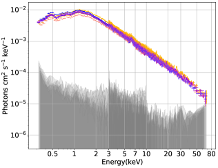
Figure 5: Background-subtracted XMM-Newton EPIC-pn and NuSTAR FPMA-B spectra and the corresponding background levels (shaded regions). The simultaneous XMM-Newton and NuSTAR observations are reported with the same color. The color code for different observations is the same as in Fig. 3. This color code is applied throughout the paper.

We performed the spectral analysis using the xspec v.12.12.1 software package (Arnaud 1996). The spectra obtained by the two NuSTAR modules (FPMA and FPMB) are fitted simultaneously, with a cross-normalization constant typically less than 5% (Madsen et al. 2015).

Errors and upper/lower limits are calculated using $\Delta\chi^{2}$ = 2.71 criterion (corresponding to the 90% confidence level for one parameter), unless stated otherwise.

The Galactic column density at the position of the source ($N_{\rm H}=4.1\times 10^{20}\rm cm^{-2}$, HI4PI Collaboration et al. 2016) is always included in the fits, and it is modeled with the tbabs component (Wilms et al. 2000) in xspec, with $N_{\rm H}$ kept frozen to the quoted value. We also assumed Solar abundances, unless stated otherwise.

Fig. 5 shows the background subtracted EPIC pn (0.3–10 keV), and FPMA-B spectra (3–75 keV), plotted with the corresponding X-ray background. In all figures, the spectra have been corrected for the effective area of each detector.

4.1 XMM-Newton data analysis

We started our spectral analysis with the 2022 EPIC-pn XMM-Newton spectra (in the 0.3–10 keV range). We fitted the spectra separately, adopting a fitting model which was based on past literature results. The model is composed of a neutral absorption component at the redshift of the source, a WA component (Steenbrugge et al. 2005) and an UFO component (Markowitz et al. 2006; Tombesi et al. 2011), xspec model: tbabs * ztbabs * mtable(WAcomp) * mtable(UFOcomp) * (bbody + powerlaw + zgauss + zgauss). The two latter components are modelled with detailed grids computed using the photoionization code xstar (Kallman & Bautista 2001), with an input spectral energy distribution described by a power law with a photon index of $\Gamma=2$. These tables consider standard solar abundances from Asplund et al. (2009), and take into account absorption lines and edges for all the metals characterized by an atomic number $Z\leq 30$. Considering the typical values of turbulent velocity for WAs (Laha et al. 2014), we used a table computed considering a turbulent velocity of 100 $\rm km\,s^{-1}$ for the WA and a table computed considering a turbulent velocity of 1000 $\rm km\,s^{-1}$ for the UFO. We added a black-body component to take into account any weak underlying soft X-ray spectral feature, as the soft excess. The primary continuum is modelled by a simple power law. Since we are focusing on the XMM-Newton energy band range, we did not include reflection features at this stage. Two Gaussian lines are included, to represent the iron K$\alpha$ and K$\beta$ lines. The line widths of both lines are free to vary, as well as their centroid energies. The fits obtained using this model are very good (see left panels of Fig. 6). The values of the Fe K$\alpha$ line parameters are shown in Table 2. The line width of the Fe K$\beta$ line is $\sim 80-90$ eV because it is fitting a blend of lines which could include also Fe xxvi . The line width of the Fe K$\alpha$ line in some observations is unconstrained, and we found only upper limits. In all observations, the line width of the K$\alpha$ line is always below $100$ eV. This suggests that if there is a broad component of the Fe K$\alpha$ line it was not detectable during our X-ray monitoring campaign.

Table 2: Details of the iron K$\alpha$ line parameters from the analysis of the XMM-Newton observations. The flux of the Fe K$\alpha$ line is given in unit of $\rm erg\,\rm cm^{-2}\,\rm s^{-1}$ .

Obs.ID	E[keV]	$\sigma$[eV]	EW [eV]	$\log(F)$
0862090101	$6.39\pm 0.03$	$<92$	$64\pm 12$	$-12.12\pm 0.08$
0862090201	$6.36\pm 0.02$	$65_{-32}^{+99}$	$96\pm 15$	$-12.03\pm 0.08$
0862090301	$6.36\pm 0.01$	$93_{-17}^{+132}$	$112\pm 18$	$-12.02\pm 0.07$
0862090501	$6.37\pm 0.02$	$<82$	$46\pm 9$	$-12.30\pm 0.08$
0862090601	$6.36\pm 0.02$	$81_{-42}^{+122}$	$115\pm 23$	$-11.97\pm 0.10$
0862090701	$6.38\pm 0.02$	$<48$	$81\pm 19$	$-12.09\pm 0.12$
0862090801	$6.38\pm 0.02$	$87_{-54}^{+114}$	$104\pm 26$	$-12.01\pm 0.07$
0862090901	$6.35\pm 0.03$	$69_{-35}^{+132}$	$78\pm 29$	$-12.14\pm 0.11$
0862091001	$6.39\pm 0.02$	$99_{-66}^{+131}$	$108\pm 31$	$-11.99\pm 0.07$

In the soft energy band (0.3–2 keV) we found the presence of a moderate soft excess component with temperatures ranging from kT${}_{\rm BB}=47\pm 15$ eV to kT${}_{\rm BB}=75\pm 6$ eV and a neutral absorption component at the redshift of the source with $N_{\rm H}=(2.67\pm 0.07)\times 10^{21}\,$cm^-2 over the 9 XMM-Newton observations. We also confirmed the presence of two X-ray ionized absorbing components, consistent with previous studies (Steenbrugge et al. 2005; Markowitz et al. 2006; Tombesi et al. 2011). These components are constant within their uncertainties during the monitoring. We found for the X-ray wind with turbulent velocity 100 $\rm km\,s^{-1}$, identified with a warm absorber, an average column density $N_{\rm H}=(1.49\pm 0.16)\times 10^{21}\,$cm^-2 , an average ionization fraction $\log(\xi/\rm erg\,\rm s^{-1}\rm cm)=1.30\pm 0.07$ and an average observed redshift of the absorption components z=$-0.011\pm 0.005$. The component with turbulent velocity 1000 $\rm km\,s^{-1}$, identified with a UFO, shows an average column density $N_{\rm H}=(1.97\pm 0.82)\times 10^{21}\,$cm^-2, an average ionization fraction $\log(\xi/\rm erg\,\rm s^{-1}\rm cm)=2.69\pm 0.03$ and an average z=$-0.177\pm 0.016$.

4.2 NuSTAR data analysis

Before analysing the broadband spectra, we first focused on the primary emission and on its reflected component using NuSTAR FPMA+B spectra (in the 3–75 keV range). During the fitting process, we left the NuSTAR FPMB cross-calibration constant free to vary. Again we composed a model following those presented in the literature (e.g. Brenneman et al. 2014a, b). We modeled the primary X-ray continuum with the cutoffpl model in xspec, which includes a power law with high energy exponential cut-off, and the reprocessed emission using the standard neutral reflection model xillver version [1.4.3] with $\log(\xi)$ fixed to zero (García et al. 2013) (xspec model: tbabs*(cutoffpl+ xillver)). The cut-off energy, $E_{\rm c}$, and the photon index, $\Gamma$, of the xillver component are linked those of the cutoffpl and the reflection fraction, $R_{\rm refl}$, is forced to be negative. With these settings, xillver reproduces only the reflection component. The disk inclination angle was fixed to a value of $60^{\circ}$ (Brenneman et al. 2014b). The data are very well reproduced by the model, the ratio between data and model are shown in the central panels of Fig. 6, in which we reported also the $\chi^{2}_{r}$ = $\chi^{2}$/degrees of freedom (dof). In this analysis, we found a photon index of the primary power law ranging from $\Gamma=1.67\pm 0.04$ to $\Gamma=1.74\pm 0.03$, and a cut-off value $E_{\rm c}=145-180$ keV in agreement with previous studies (e.g., Brenneman et al. 2014b). However, respect to the results obtained by Brenneman et al. (2014b), we found a significantly lower value for the reflection fraction, R${}_{\rm refl}=0.008-0.01$, similar to that found by the analysis of Suzaku and NuSTAR observations of IC 4329A by Ogawa et al. (2019). Together with the result of our analysis of the Fe K$\alpha$ line with the XMM-Newton observations, which shows faint broad features (see Sect. 4.1), this suggests that the reflection from the inner disk is weak.

We also tested the scenario in which the Fe K$\alpha$ emission is slightly broadened by relativistic effects and it is coming from the accretion disk by substituting the xillver component with the relxill component (García et al. 2014; Dauser et al. 2014), which takes into account ionised relativistic reflection from an accretion disk illuminated by a hot corona. This model resulted in a significantly worse fit ($\chi^{2}_{r}\sim 1.4-1.7$). Moreover, we were not able to constrain the black hole spin in any of the NuSTAR observations of this campaign, finding just a lower limit of $a\gtrsim 0.1$.

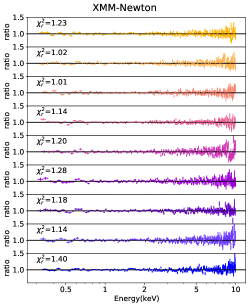
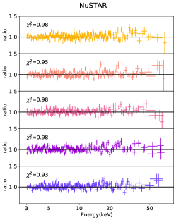
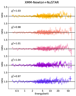
Figure 6: Data/model ratio for the EPIC-pn XMM-Newton observations (left panels), FPMA+B NuSTAR observations (central panels) and the X-ray broad-band observations (right panels) of IC 4329A when the best fitting model is applied in each case, see Sect. 4.

4.3 Broad-band data analysis

Table 3: Best fitting parameters for the X-ray broad-band XMM-Newton plus NuSTAR spectra of IC 4329A. Errors are at 90% confidence levels.

Model	Parameter	Obs.ID
		0862090101	0862090301	0862090501	0862090701	0862090901
		60702050002	60702050004	60702050006	60702050008	60702050010
Model A	$\frac{\chi^{2}}{\rm dof}=\chi^{2}_{r}$	1.03	0.98	1.01	1.04	0.97
cutoffpl	$\Gamma$	$1.71\pm 0.01$	$1.65\pm 0.02$	$1.71\pm 0.02$	$1.73\pm 0.02$	$1.77\pm 0.02$
cutoffpl	$E_{\mathrm{cut}}$(keV)	$163^{+55}_{-35}$	$140^{+56}_{-75}$	$220^{+89}_{-45}$	$249^{+70}_{-92}$	$228^{+57}_{-41}$
xillver	R refl	$0.006\pm 0.001$	$0.008\pm 0.002$	$0.006\pm 0.001$	$0.009\pm 0.002$	$0.009\pm 0.001$
xillver	A Fe	$3.41^{+1.09}_{-0.89}$	$3.72^{+2.46}_{-1.31}$	$3.77^{+1.30}_{-1.17}$	$3.1^{+1.28}_{-0.53}$	$1.91^{+1.24}_{-0.81}$
Model B1	$\frac{\chi^{2}}{\rm dof}=\chi^{2}_{r}$	1.06	1.002	1.03	1.06	1.005
cutoffpl	$\Gamma$	$1.75\pm 0.02$	$1.71\pm 0.01$	$1.73\pm 0.01$	$1.74\pm 0.02$	$1.81\pm 0.02$
cutoffpl	$E_{\mathrm{cut}}$(keV)	$>214$	$>171$	$>210$	$>245$	$>305$
mytorus	$N_{\rm H,tor}[10^{23}\rm cm^{-2}]$	$2.84\pm 0.63$	$2.78\pm 0.95$	$2.67\pm 0.48$	$2.32\pm 0.84$	$2.48\pm 0.65$
Model B2	$\frac{\chi^{2}}{\rm dof}=\chi^{2}_{r}$	1.07	1.01	1.06	1.11	1.006
RXTorusD	$\Gamma$	$1.73\pm 0.01$	$1.70\pm 0.02$	$1.73\pm 0.04$	$1.76\pm 0.01$	$1.76\pm 0.01$
RXTorusD	$N_{\rm H,tor}[10^{23}\rm cm^{-2}]$	$2.13^{+0.83}_{-0.38}$	$3.70\pm 0.51$	$2.34\pm 0.36$	$5.10\pm 0.56$	$3.57\pm 0.76$
RXTorusD	$i({\rm deg})$	$44.91\pm 0.98$	$44.66\pm 1.25$	$44.04\pm 1.66$	$44.83\pm 0.77$	$45.00\pm 0.34$
RXTorusD	$r/R$	$0.69\pm 0.02$	$0.69\pm 0.01$	$0.69\pm 0.02$	$0.69\pm 0.01$	$0.69\pm 0.03$
Model C	$\frac{\chi^{2}}{\rm dof}=\chi^{2}_{r}$	1.05	0.98	0.99	1.04	0.98
xillverCp	$\Gamma$	$1.77\pm 0.01$	$1.76\pm 0.03$	$1.80\pm 0.02$	$1.80\pm 0.01$	$1.82\pm 0.02$
xillverCp	kTe(keV)	$78^{+32}_{-26}$	$75^{+54}_{-61}$	$>135$	$>175$	$>175$
xillverCp	R refl	$<3.37$	$1.45\pm 0.62$	$<0.82$	$0.16\pm 0.04$	$<0.96$
xillverCp	A Fe	$>3.74$	$>1.59$	$1.01^{+0.85}_{-0.25}$	$0.87^{+0.63}_{-0.16}$	$<0.50$
xillverCp	$\log(N_{\rm H,disk}/\rm cm^{-2})$	$18.01^{+1.57}_{-0.64}$	$19.18^{+0.69}_{-1.09}$	$<16.20$	$<17.21$	$>15.03$
F${}_{2-10}(10^{-11}$ $\rm erg\,\rm cm^{-2}\,\rm s^{-1}$ )		$11.04\pm 0.24$	$7.79\pm 0.53$	$9.09\pm 0.29$	$8.64\pm 0.36$	$8.49\pm 0.27$

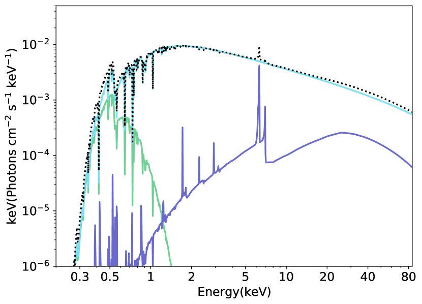
Figure 7: Model A (see Sect. 4.3). The black dotted line represents the total model, which is composed of the primary X-ray emission (light blue line), the reprocessed component (dark blue line) and the soft excess component (green line). Absorption and emission features are included in the model.

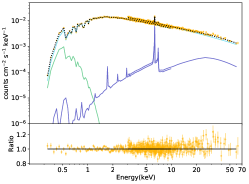
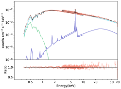
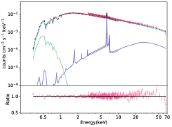
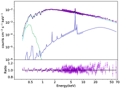
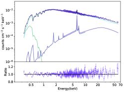
Figure 8: Unfolded data plus fitting model (upper panels) and ratio residuals (lower panels) for the X-ray broad-band observations of IC 4329A when the best fitting model is applied. We show all the model components as in Fig. 7, see Sect. 4 for more details.

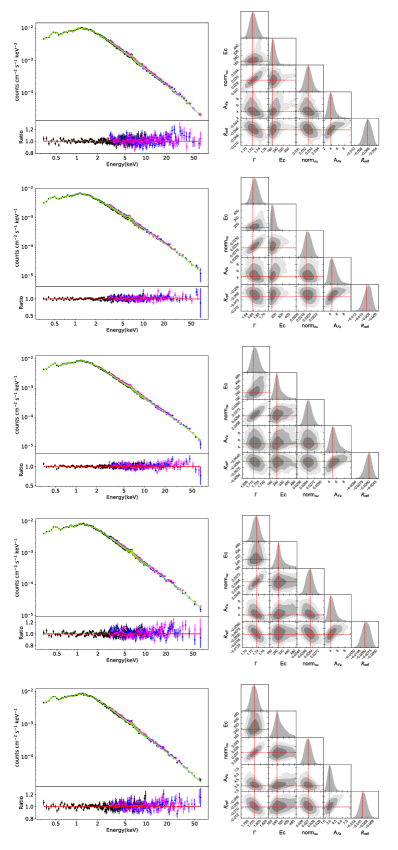
Figure 12: Left panels: data, fitting model and residuals ratio for XMM-Newton EPIC-pn (black) and NuSTAR FPMA (blue) and FPMB (magenta) spectra of the simultaneous observations of IC 4329A when Model A (see Sect. 4.3) is applied to the data. Right panels: 68%, 90% and 99% contour plots resulting from the MCMC analysis of the Model A applied to the broad-band XMM-Newton and NuSTAR 0.3–75 keV spectra of IC 4329A. We show the outputs for photon index ($\Gamma$), cut-off energy ($E_{\mathrm{cut}}$[keV]), NuSTAR normalization (nor$M_{\rm nu}$ [ph/keV/cm²/s]), iron abundance ($A_{\rm Fe}$), and reflection fraction ($R_{\rm refl}$). We reported from top to bottom the Obs.ID:086209101+60702050002,086209103+60702050004,086209105+60702050006,086209107+60702050008,086209109+60702050010.

Finally, we extended the analysis to include the whole 0.3–10 keV XMM-Newton EPIC-pn spectrum and the 3–75 keV NuSTAR FPMA/FPMB spectra for the simultaneous observations (see Table 1). For the spectral fitting we used the following xspec model: tbabs * ztbabs * mtable(WAcomp) * mtable(UFOcomp) * (bbody + cutoffpl + xillver) (hereafter Model A, see Fig. 7) which is the combination of the previous models. The data/model ratio of this analysis and the resulting $\chi^{2}_{r}$ are shown in the right panels of Fig. 6. We show data, fitting model and residuals ratio for all the simultaneous XMM-Newton and NuSTAR observations in Fig. 12.

Even if from the analysis of the XMM-Newton data the Fe K$\alpha$ line does not seems to be broad, we carried out additional tests to confirm this result. The xillver model accounts for the narrow Fe K$\alpha$ emission line so we included Gaussian line, for a broad component. Indeed this component was not necessary as its normalisation was unconstrained, and we only found an upper limit of $\sim 10^{-7}$ ph cm^-2 s^-1 in all the observations, with an upper limit on the equivalent width in the range of 5–10 eV. We reported the best fitting parameters for the X-ray primary continuum ($\Gamma$ and E_c) and the reflection component (A_Fe and R_refl) in Table 3.

The very low value of the reflection fraction and the faint broad component of the Fe K$\alpha$ line in the fit of the broad-band spectra give strength to the hypothesis in which the disk reflection is weak and the narrow iron K$\alpha$ signature is coming from distant material (see Sect. 5.2). To further test this scenario, we replaced the xillver with the mytorus model (Murphy & Yaqoob 2009), to reproduce the reflection from distant neutral material (Model B1). The inclination angle of the torus was fixed at 30^∘. To reproduce the Compton-scattered continuum we used a table in which the termination energy is fixed by default in the Model and is 160 keV, the closest value to the cut-off energy found with Model A. To reproduce the fluorescent line spectra we used another table with line centroid offset $E_{\rm off}=0$ keV and with the same termination energy as the previous one. The column densities of the scattered and line components were linked and free to vary. The normalisation of the scattered and line components were tied to the normalization of the primary continuum, i.e. the standard mytorus configuration (the so-called ’coupled’ reprocessor; see e.g. Yaqoob 2012). The assumed geometry corresponds to a covering fraction of 0.5.

The statistical significance of the fits with Model B1 is similar to that of Model A. We found a value for the average column density of the torus of $2.6\times 10^{23}$ cm^-2 consistent within the errors with the results obtained for all the observations of this campaign (see Table 3). The photon index values obtained for the primary continuum are consistent within the errors with those obtained with Model A but we were not able to constrain the cut-off energies, most likely because of the degeneracies among the parameters. Moreover, mytorus does not include a cut-off energy but a termination energy which is fixed to be 160 keV. We reported the best-fitting parameters of Model B1 in Table 3.

Additionally, we also tested the reflected emission from a dusty torus with variable covering fraction (Model B2) using the RXTorusD model (Paltani & Ricci 2017; Ricci & Paltani 2023), the first torus model to consider dusty gas. In these tables the cutoff energy is fixed to 200 keV, which is a value consistent with the value of $E_{\rm c}$ we found in IC 4329A (See Table 3). The level of statistical significance observed in the fits using Model B2 is comparable to that observed using Model B1. Also the values of the photon index and the equatorial column density of the torus are comparable within the errors with the ones of Model B (see Table 3). With Model B2 we were able to measure the inner-to-outer radius ratio of the torus, i.e. $r/R=0.69\pm 0.02$, and the viewing angle $i\sim 45^{\circ}$. These values were constant among the observations. All the parameters values are reported in Table 3.

The results obtained with Model A, B1 and B2 are consistent with the iron K$\alpha$ line originating from neutral Compton-thin ($N_{H}=10^{22}-10^{23}$ cm^-2) material which does not produce a prominent Compton reflection.

We searched for possible degeneracies between the fitting parameters in Model A, performing Monte Carlo Markov Chain (MCMC) using the xspec-emcee tool. This is an implementation of the emcee code (Foreman-Mackey et al. 2013), to analyze X-ray spectra within xspec. We used 50 walkers with 10000 iterations each, burning the first 1000. The walkers started at the best fit values found in xspec, following a Gaussian distribution in each parameter, with the standard deviation set to the delta value of that parameter. In the right panels of Fig. 12 the contour plots are shown, resulting from the MCMC analysis of the Model A applied to the broad-band 0.3–75 keV spectra of IC 4329A.

To directly measure the coronal temperature parameter we used the xillverCp versions of the xillver tables (Model C). This model assumes that the primary emission is due to the Comptonization of thermal disc photons in a hot corona and the reflection spectrum is calculated by using a more physically motivated primary continuum, implemented with the analytical Comptonization model nthcomp (Zdziarski et al. 1996; Życki et al. 1999), instead of a simple cut-off power law. The seed photon temperature is fixed at 50 eV by default in this model. This value is consistent with the maximum disk temperature expected for a source with $M_{\rm BH}=6.8^{+1.2}_{-1.1}\times 10^{7}M_{\odot}$ (Bentz et al. 2023) (i.e. $T_{\rm Wien}=32\pm 10$ eV). As reported in Table 3, we were able to constrain the coronal temperature just for two observations. The electron temperature of the corona is thought to be related to the spectral cut-off energy, $E_{c}\sim 2-3\times kT_{\rm e}$ (Petrucci et al. 2000, 2001). Assuming this relation, the values we obtained with Model C for the electron temperature of the corona are consistent with the cut-off values that we obtained with Model A.

4.4 Re-analysis of the past observations

Table 4: Summary of the previous XMM-Newton , NuSTAR and Suzaku observations of IC 4329A.

Telescope	Obs. ID	Start Date	Exp
		yyy-mm-dd	ks
XMM-Newton	0101040401	2001-01-31	13.9
XMM-Newton	0147440101	2003-08-06	136.1
Suzaku	0702113010	2007-08-01	25.4
Suzaku	0702113020	2007-08-06	30.6
Suzaku	0702113030	2007-08-11	26.9
Suzaku	0702113040	2007-08-16	24.2
Suzaku	0702113050	2007-08-20	24.0
NuSTAR	60001045002	2012-08-12	162.4
Suzaku	0707025010	2012-08-13	117.4
XMM-Newton	08800760801	2018-01-08	16.4

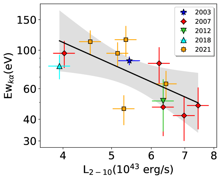
Figure 9: Top panel: The equivalent width (EW_Kα) of the neutral iron line plotted against 2–10 keV X-ray luminosity ($L_{\rm 2-10}$). The black lines is the linear regressions while the shaded black regions represent the combined 3$\sigma$ error on the slope and normalisation.

Table 5: Best fitting parameters of the primary continuum and details of the iron K$\alpha$ line parameters for the analysis of the spectra of IC 4329A from the past XMM-Newton and Suzaku observations as in Table 4. Errors are at 90% confidence levels. The FeK$\alpha$ flux and the 2–10 keV flux are given in unit of $\rm erg\,\rm cm^{-2}\,\rm s^{-1}$ .

Obs.ID	kTBB[keV]	$\Gamma$	$E_{\rm FeK\alpha}$[keV]	$\sigma_{\rm FeK\alpha}$[eV]	EWFeKα [eV]	$\log(F_{K\alpha})$	$\log(F_{2-10})$	$\chi^{2}_{r}$
0101040401	$0.08\pm 0.01$	$1.68\pm 0.08$	-	-	-	-	$-9.46\pm 0.55$	0.97
0147440101	$0.42^{*}\pm 0.01$	$1.71\pm 0.01$	$6.35\pm 0.04$	$96\pm 17$	$87\pm 5$	$-12.12\pm 0.03$	$-10.03\pm 0.01$	1.74
0702113010	$0.08\pm 0.05$	$1.84\pm 0.01$	$6.38\pm 0.03$	$115\pm 32$	$84\pm 20$	$-11.98\pm 0.07$	$-9.97\pm 0.03$	1.04
0702113020	$0.03\pm 0.02$	$1.88\pm 0.02$	$6.40\pm 0.02$	$82\pm 12$	$48\pm 12$	$-12.32\pm 0.07$	$-9.89\pm 0.01$	1.10
0702113030	$0.07\pm 0.01$	$1.77\pm 0.01$	$6.37\pm 0.04$	$71\pm 6$	$42\pm 12$	$-12.08\pm 0.08$	$-9.92\pm 0.03$	1.08
0702113040	$0.07\pm 0.01$	$1.85\pm 0.01$	$6.39\pm 0.04$	$78\pm 4$	$47\pm 15$	$-12.15\pm 0.10$	$-9.96\pm 0.04$	1.06
0702113050	$0.06\pm 0.01$	$1.74\pm 0.01$	$6.36\pm 0.05$	$67\pm 10$	$96\pm 21$	$-12.41\pm 0.12$	$-10.16\pm 0.01$	1.04
0707025010	$0.06\pm 0.02$	$1.75\pm 0.01$	$6.36\pm 0.06$	$77\pm 14$	$51\pm 27$	$-12.04\pm 0.03$	$-9.96\pm 0.01$	1.10
08800760801	$0.11\pm 0.05$	$1.63\pm 0.03$	$6.39\pm 0.03$	$<140$	$81\pm 13$	$-11.91\pm 0.03$	$-10.17\pm 0.24$	0.93

^∗ The higher value of the kT_BB of this Obs.ID is not related to the variability of the soft excess but it is most likely due to the higher $N_{H}$ value of the UFO component (see Table  6 that could drive the black body shape of the soft excess).

To better understand the origin of the Fe K$\alpha$ line, the evolution of the spectral parameters of the primary continuum and of the soft energy components (e.g., soft-excess or outflowing components) we compared the results of our campaign with those obtained by previous observations of IC 4329A (see Table 4). This was done by re-analysing the archival XMM-Newton (2001, 2003, 2018), NuSTAR (2012) and Suzaku (2007, 2012) data. In Fig. 10 we show the 2–10 keV flux of IC 4329A during the years including the literature values from observations carried out in the past four decades. During this period, the 2–10 keV flux of IC 4329A has changed by a factor $\sim 2.1$. The highest state was in 2001 when the flux was F${}_{\rm 2-10}=1.75\times 10^{-10}$ $\rm erg\,\rm cm^{-2}\,\rm s^{-1}$ while in 2001 the source reached the lowest state with F${}_{\rm 2-10}=8.15\times 10^{-11}$ $\rm erg\,\rm cm^{-2}\,\rm s^{-1}$ , $\sim 70$% lower than the value of 2007.

We applied the same fitting approach outlined in Sect. 4.1 to the archival XMM-Newton observations and to the 2007 Suzaku observations, while we used Model A (see Sect. 4.3) to fit the simultaneous NuSTAR and Suzaku observations of 2012.

The continuum emission of all the past XMM-Newton observations and of the Suzaku observations of 2007 is well fitted by a power law and a black-body component, the latter being included to take into account the soft excess. The simultaneous NuSTAR and Suzaku observations of 2012 are well fitted by Model A (see Sect. 4.3). From the analysis of these simultaneous observations we found a primary power law characterized by a photon index $\Gamma=1.74\pm 0.01$ and an exponential cut-off at E${}_{c}=173\pm 13$ keV in agreement with what was found by Brenneman et al. (2014b). We also found an iron abundance A${}_{\rm Fe}=1.08\pm 0.22$ and a low value of the reflection fraction: R${}_{\rm refl}=0.009\pm 0.004$, in agreement with the results obtained from our monitoring campaign (see Sect. 4.3 and Table 3). We report the values of the best fitting parameters of the primary continuum for the XMM-Newton and Suzaku observation in Table 5. Data, fitting models and residuals ratio are shown in Fig. 12. Moreover, all these observations, as well as the Suzaku observation from 2012, show the presence of a WA and an UFO components, except the XMM-Newton observation from 2001, for which the presence of ionized absorbers could not be assessed due to the low SNR. The values of the parameters of these components are reported in Table 6. Since during the 2007 Suzaku monitoring (5 observations, each $\sim 5$ ks long) the spectral parameters values are constant within the errors, we report the average values. For a consistent analysis we also applied to the XMM-Newton observation of 2003 the same model as in Tombesi et al. 2011 (i.e., a power law component absorbed by Galactic column density and a xstar table with the turbulent velocity of 1000 $\rm km\,s^{-1}$ to the 4–10 keV band). We found values similar to those reported in Tombesi et al. 2011: $N_{H}=(1.69\pm 0.23)\times 10^{22}$ cm^-2, $\log(\xi/\rm erg\,\rm s^{-1}\rm cm)=4.23\pm 0.82$, $v_{\rm w}/c=0.095\pm 0.004$.

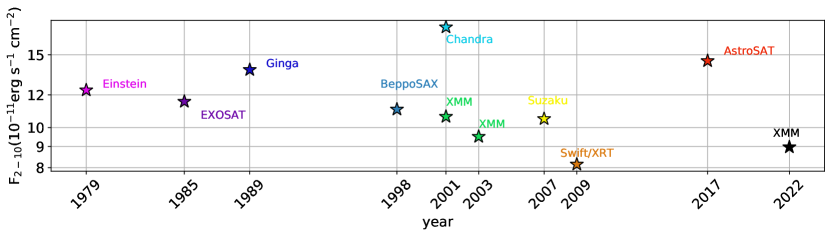
Figure 10: The historical 2–10 keV light curve of IC 4329A as observed with various X-ray satellites. In chronological order: Einstein, 1979 (Holt et al. 1989); EXOSAT, 1985 (Singh et al. 1991); Ginga, 1989 (Piro et al. 1990); BeppoSAX, 1998 (Dadina 2007); Chandra, 2001 (Shu et al. 2010a); XMM-Newton 2001, 2003 (Nandra et al. 2007); Suzaku , 2007 (Mantovani et al. 2014); Swift/XRT, 2007 (Winter et al. 2009); AstroSat, 2017 (Tripathi et al. 2021); XMM-Newton 2022, medium flux of the observations analysed in this work.

Additionally, we found the values of the equivalent width (EW_Kα) of the FeK$\alpha$ line obtained from the old observation and from the observations of the 2021 campaign, to be inversely correlated with the X-ray luminosity in the 2–10 keV band. Fitting these two parameters with a linear regression we found a marginally significant ($2.8\sigma$) anti-correlation with Pearson correlation coefficient $\rho=-0.664$ (see Fig. 9). This trend is known as the ‘X-ray Baldwin’ or ‘Iwasawa-Taniguchi’ effect (hereafter ‘IT effect’) (Iwasawa & Taniguchi 1993). This inverse correlation is similar to the classical ’Baldwin effect’, in which the equivalent width of the [C IV] $\lambda$1550 emission line is inversely correlated with the UV continuum luminosity (Baldwin 1977). The IT effect has been found in a large sample of different objects studied with different instruments (Page et al. 2004; Jiang et al. 2006; Bianchi et al. 2007; Shu et al. 2010b; Ricci et al. 2014). Several explanations have been proposed for the IT effect: the decrease in covering factor of the material forming the FeK$\alpha$ line (Page et al. 2004; Ricci et al. 2013), the dependency from the luminosity of the ionisation state of the material which produce the line (Nandra et al. 1997b; Nayakshin 2000), the variability related to the non-simultaneous reaction to flux changes of the continuum of the reprocessing material (Jiang et al. 2006). One notable distinction we found in the re-analysis of the past observations of IC 4329A is the lack of a distinct broad component of the iron line. Excluding the XMM-Newton observation of 2001 in which it was not possible to detect the FeK$\alpha$ line for the low SNR ratio of the observation, the other observations show a low value for both the line width and equivalent width of the broad component of the FeK$\alpha$ (see Table 5).

5 Discussion

5.1 Spectral Variability

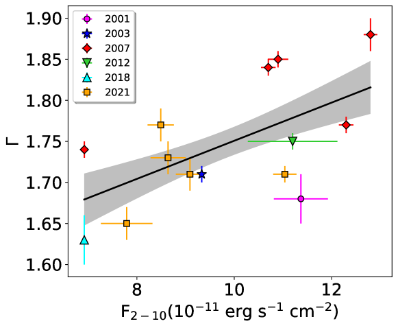
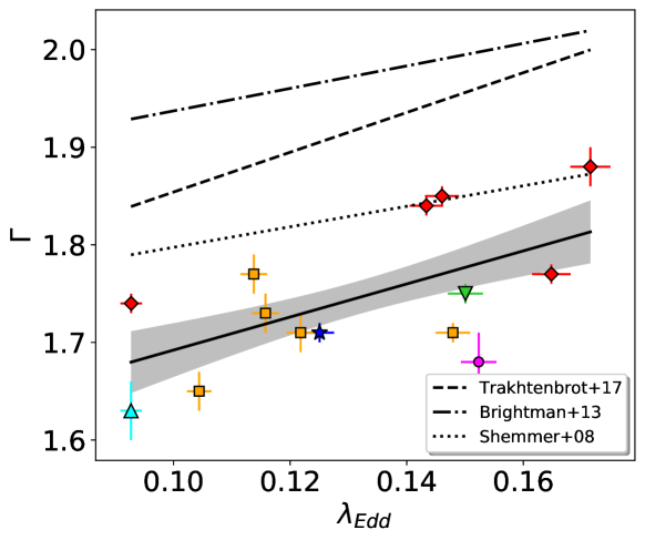
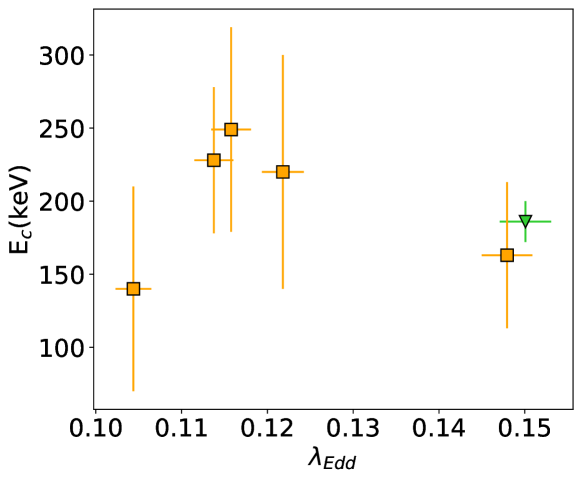
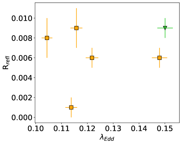
Figure 11: Top panels: $\Gamma$ vs F${}_{\rm 2-10\,keV}$ (left) and $\Gamma$ vs $\lambda_{\rm Edd}$ (right) relation for IC 4329A. The black lines is the linear regressions while the shaded black regions represent the combined 1$\sigma$ error on the slope and normalisation. On the right panel the dotted, dotted dashed and dashed lines represent respectively the relations from Shemmer et al. (2008), Brightman et al. (2013) and Trakhtenbrot et al. (2017). Bottom left panel: E_c vs $\lambda_{\rm Edd}$. Bottom right panel: R_refl vs $\lambda_{\rm Edd}$. The plots include the data from our campaign and data obtained from archival XMM-Newton , NuSTAR and Suzaku observations. E_c and R_refl can not be measured if there are just XMM-Newton data available. The Eddington ratio are computed using the bolometric luminosity estimated using the bolometric correction to the 2–10 keV X-ray luminosity ($\kappa_{2-10}$) from Lusso et al. (2010)

The continuum 2–10 keV flux of IC 4329A showed fluctuations over the past 43 years (Fig. 10) and we also observed significant variability during our campaign. In fact the maximum value of the observed 2–10 keV flux in our monitoring is $\sim$30% larger than the minimum observed value (see Table  3). Consequently, we aimed to investigate whether the spectral properties of the sources are connected to the flux level of the source. The photon index of the power law shows some evidence for variability between the different observations. Including the values from archival observations, we found that $\Gamma$ shows a moderate correlation with the 2–10 keV flux with a Pearson correlation coefficient of 0.63 corresponding to a $1-P_{\rm value}$ of 98%, see top left panel of Fig. 11. This is in agreement with the softer-when-brighter behavior typically observed in AGN (Sobolewska & Papadakis 2009; Trakhtenbrot et al. 2017). Specifically, it has been found that as the 2–10 keV flux increases, the photon index tends to become steeper (Shemmer et al. 2006). This could be related to changes in the physical conditions of the accretion disk as the flux increases (Haardt & Maraschi 1991), or to the effect of pair production in the X-ray corona (Ricci et al. 2018).

Several studies during the past decades have shown that $\Gamma$ is strongly correlated with $\lambda_{\rm Edd}$ (Lu & Yu 1999; Wang et al. 2004; Shemmer et al. 2006, 2008; Brightman et al. 2013; Trakhtenbrot et al. 2017). We checked the presence of this correlation between the values of the photon index of IC 4392A found in our monitoring and from archival observations, with the Eddington ratio computed using the bolometric luminosity estimated using the bolometric correction to the 2–10 keV X-ray luminosity ($\kappa_{2-10}$) from Lusso et al. (2010). We found a moderate $\Gamma$ vs $\lambda_{\rm Edd}$ correlation (Pearson correlation coefficient $\rho_{\rm corr}=0.62$, corresponding to a $1-P_{\rm value}$ of 97%, see top right panel of Fig. 11). The linear regression has a slope value of $1.69\pm 0.80$ which is consistent within the errors with the values expected from the literature (e.g. Shemmer et al. 2008; Brightman et al. 2013; Trakhtenbrot et al. 2017) but with a lower normalisation value: $1.52\pm 0.11$.

This result implies that IC 4329A fits well the picture in which the mass accretion rate is responsible for driving the physical conditions of the AGN corona, responsible for the shape of the X-ray spectrum. Therefore the cut-off energy is expected to show a correlation with the 2–10 keV flux/luminosity and with the Eddington ratio. In Tortosa et al. (2018) we did not find a clear evidence of a significant correlation between $E_{\rm c}$ and $\lambda_{\rm Edd}$ in the sample of bright AGN observed at the time with NuSTAR . However, the sample was still small, and did not allow the exclusion of the existence of this kind of relation. Ricci et al. (2018), using the values from the BASS X-ray catalogue (Ricci et al. 2017), found a negative correlation in the $E_{\rm c}$ vs $\lambda_{\rm Edd}$ relation suggesting that the Eddington ration is the main parameter driving the cut-off energy in AGN. The high energy cut-off values of IC 4329A are marginally different among the observations, but still consistent within the errors with previous literature values (Brenneman et al. 2014b) and with the median values of bright nearby AGN (Ricci et al. 2018). We do not observe a clear correlation in this monitoring between this parameter and $\lambda_{\rm Edd}$ (see lower panels of Fig. 11).

Among the different observations of our campaign, the reflection fraction is consistent with being constant within the errors (see lower right panel of Fig. 11). This parameter shows a very low value, consistent with what has been observed in the analysis of Suzaku and NuSTAR observations of IC 4329A by Ogawa et al. (2019). This result, in addition to our analysis of the Fe K$\alpha$ line based on XMM-Newton observations, which shows faint broad features (see Sect. 4.1), suggests that the reflection from the inner disk is weak. This interpretation is further supported by the fact that the narrow features of the iron line seen in the XMM-Newton observations are consistent with being associated to emission from distant neutral material.

IC 4329A shows also a clear presence of a moderate soft excess component. However this component does not vary among the observations. It has a temperature ranging from kT${}_{\rm BB}=68\pm 5$ eV to kT${}_{\rm BB}=75\pm 6$ eV, consistent within the error among the observations of this campaign and with the temperature found analysing the archival observations (see Table  4). The flux of the soft excess component is constant among the observations of our campaign, being $(2.31-2.89)\pm 0.75\times 10^{-4}$ ph cm^-2 s^-1.

5.2 The Fe K$\boldsymbol{\alpha}$ line

The central energy of the Gaussian line in our analysis is always consistent, within the errors, with low-ionization or neutral material among all the observations of this campaign (see Table2). In fact, IC 4329A is well known to exhibit the presence of a strong Fe K$\alpha$ line (Piro et al. 1990) with a narrow core at $6.4$ keV. A broad component, most likely produced in the inner part of the accretion disc and blurred by general relativistic effects, has been found in some X-ray observations (Done et al. 2000; Dadina 2007; Brenneman et al. 2014b; Mantovani et al. 2014). Our modelling of the observations of this campaign and of the past archival observations does not need a relativistic broad component of the Fe K$\alpha$ line.

Using the mean value of the measured $\sigma_{\rm FeK\alpha}$, without considering the upper limits (see Table 2) we computed a full width at half-maximum (FWHM) of the iron K$\alpha$ line: FWH$M_{\rm FeK\alpha}=907\pm 132$ $\rm km\,/s$. With this value, we estimated the radius of the iron K$\alpha$ line emission, assuming that the line width represents the Keplerian velocity emitting material, using the following equation:

$$R_{\rm FeK\alpha}=\frac{G\,M_{\rm BH}}{v^{2}}$$ (3)

where $G$ is the gravitational constant and $M_{\rm BH}$ is the central supermassive black hole mass (Netzer 1990; Peterson et al. 2004) and assuming a spherical geometry and an isotropic velocity distribution which results in the assumption of $v=\sqrt{3}/2v_{\rm FWHM}$. We obtained $R_{\rm FeK\alpha}=0.48\pm 0.14$ pc. As in Nandra (2006); Gandhi et al. (2015), we can compare the radial position of the iron K$\alpha$ line emitting region with the optical BLR radius R_Hβ, inferred from H$\beta$ reverberation studies, and with the value of the dust sublimation radius R_sub (i.e., inner radius of the dusty torus, Nenkova et al. 2008). R_sub is defined as:

$$R_{\rm sub}=0.4\left(\frac{L_{\rm bol}}{10^{45}\rm{ergs^{-1}}}\right)^{0.5}\left(\frac{1500\,K}{T_{\rm sub}}\right)^{2.6}[pc]$$ (4)

where $L_{\rm bol}$ is the bolometric luminosity and $T_{\rm sub}$ is the dust sublimation temperature, assumed to be the sublimation temperature of graphite grains ($T\sim 1500$ K, Kishimoto et al. 2007). Considering a bolometric luminosity of $\log(L_{\rm bol}/\rm erg\,s^{-1})=45.04$ (Koss et al. 2017), we obtain R${}_{\rm sub}=0.42$ pc while R${}_{\rm H\beta}=0.012$ pc from both Bentz et al. 2009, 2023. Looking at these values, the bulk of the Fe K$\alpha$ emission line of IC 4329A appears to likely originate in the dusty torus. This finding is also consistent with the value of the dust-continuum size ($0.14\pm 0.01$ pc) found by Gravity Collaboration et al. (2023).

5.3 X-ray outflows

Table 6: Spectral parameters, velocity, upper and lower limits on the radial location and upper limits on the energetic parameters for each X-ray absorber during the years.

$v_{\rm turb}=100$ $\rm km\,s^{-1}$	2003	2007	2012	2018	2021
$N_{\rm H}(10^{21}\rm cm^{-2})$	$1.35\pm 0.01$	$1.42\pm 0.16$	$1.03\pm 0.37$	$1.75\pm 0.72$	$1.49\pm 0.16$
$\log(\xi/\rm erg\,\rm s^{-1}\rm cm)$	$1.28\pm 0.08$	$1.54\pm 0.08$	$1.78\pm 0.03$	$1.70\pm 0.67$	$1.30\pm 0.07$
$z_{\rm obs}$	$-0.003\pm 0.001$	$-0.016\pm 0.011$	$-0.025\pm 0.009$	$-0.024\pm 0.056$	$-0.011\pm 0.005$
$v_{\rm w}/c$	$0.02\pm 0.01$	$0.03\pm 0.01$	$0.04\pm 0.01$	$0.04\pm 0.05$	$0.03\pm 0.05$
$r_{\mathrm{min}}[10^{-2}\mathrm{pc}]$	$1.18\pm 0.01$	$0.63\pm 0.04$	$0.38\pm 0.01$	$0.40\pm 0.01$	$0.88\pm 0.03$
$r_{\mathrm{max}}[\mathrm{pc}]$	$1586\pm 13$	$828\pm 93$	$657\pm 236$	$465\pm 164$	$1372\pm 147$
$\dot{M}_{\rm max}/\dot{M}_{\rm acc}$	0.38	0.24	0.13	0.24	0.30
$\dot{p}_{\rm max}/\dot{p}_{\rm rad}$	0.80	1.27	1.21	1.38	1.56
$\dot{K}_{\rm max}/L_{\rm b,out}$	0.76	2.04	2.49	2.78	2.12
Pnull	2.15E-6	3.25E-7	4.63E-5	2.74E-5	4.39E-6
$v_{\rm turb}=1000$ $\rm km\,s^{-1}$	2003	2007	2012	2018	2021
$N_{\rm H}(10^{21}\rm cm^{-2})$	$6.68\pm 0.19$	$2.58\pm 0.04$	$2.29\pm 0.22$	$1.49\pm 0.02$	$1.97\pm 0.82$
$\log(\xi/\rm erg\,\rm s^{-1}\rm cm)$	$2.44\pm 0.05$	$2.15\pm 0.09$	$2.15\pm 0.03$	$2.02\pm 0.11$	$2.69\pm 0.03$
$z_{\rm obs}$	$-0.083\pm 0.001$	$-0.076\pm 0.011$	$-0.086\pm 0.010$	$-0.094\pm 0.020$	$-0.177\pm 0.016$
$v_{\rm w}/c$	$0.102\pm 0.001$	$0.094\pm 0.011$	$0.105\pm 0.011$	$0.114\pm 0.022$	$0.207\pm 0.019$
$r_{\mathrm{min}}[10^{-4}\mathrm{pc}]$	$6.19\pm 0.13$	$7.22\pm 0.16$	$5.82\pm 0.12$	$4.97\pm 0.19$	$1.50\pm 0.28$
$r_{\mathrm{max}}[\mathrm{pc}]$	$55.27\pm 3.91$	$11.94\pm 1.73$	$126.12\pm 12.16$	$261.48\pm 3.52$	$42.28\pm 17.60$
$\dot{M}_{\rm max}/\dot{M}_{\rm acc}$	0.77	0.44	0.30	0.20	0.39
$\dot{p}_{\rm max}/\dot{p}_{\rm rad}$	1.63	2.72	3.38	5.35	3.78
$\dot{K}_{\rm max}/L_{\rm b,out}$	8.34	12.92	17.85	30.54	39.32
Pnull	9.56E-8	5.34E-9	2.13E-9	7.26E-8	1.42E-8

During the fitting process we took into account ionized absorption by including two xstar tables, as outlined in Sect. 4.1. The resulting parameters for the absorption components obtained by our analysis of the 2021 campaign, together with the results obtained for the archival observations, are listed in Table 6.

Following the same approach outlined in different studies (e.g. Tombesi et al. 2013; Serafinelli et al. 2019; Tortosa et al. 2022), we computed upper and lower bounds on the radial position of the absorbers. The lower limit on the radial location of the outflows can be placed by estimating the radius at which the observed velocity equals the escape velocity: $r_{\mathrm{min}}=2GM_{\rm BH}v^{-2}$. The upper limit is placed using the definition of the ionization parameter $\xi=L_{\rm ion}/nr^{2}$ (Tarter et al. 1969) where $L_{\rm ion}$ is the unabsorbed ionizing luminosity emitted by the source between 1 Ryd and 1000 Ryd (1 Ryd = 13.6 eV), $n$ is the number density of the absorbing material and $r$ is the distance from the central source. To apply this definition we need to assume that the thickness of the absorber does not exceed the distance from the SMBH, thus that the absorbers are somewhat compact (Crenshaw & Kraemer 2012; Tombesi et al. 2013): $r_{\mathrm{max}}=L_{\mathrm{ion}}N_{\rm H}^{-1}\xi^{-1}$ with $N_{\rm H}$ and $\xi$ respectively the column density and the ionization fraction of the absorber. We computed the ionizing luminosity using the luminosity task in xspec on the unabsorbed best fit spectral model (see Sect. 4 and Sect. 4) between 13.6 eV and 13.6 keV for all the observations.

The values of the estimated radial location of the absorber components in IC 4329A are reported in Table 6. Comparing these values with the literature it is possible to see that the outflow component with turbulent velocity 100 $\rm km\,s^{-1}$ (hereafter Wind 1) shows the typical upper and lower limits of the distance of the WAs for the type 1 Seyfert galaxies (Tombesi et al. 2013) while the outflow component with turbulent velocity 1000 $\rm km\,s^{-1}$ (hereafter Wind 2) is within the range of the average locations of ultra-fast outflows ($\sim 3\times 10^{-4}-3\times 10^{-2}$ pc, see Tombesi et al. 2012).

Regarding the outflow energetics, we computed the mass outflow rate: $\dot{M}_{\rm out}=4\pi rN_{\rm H}\mu m_{p}C_{g}v_{\rm w}$ (Crenshaw & Kraemer 2012), where $r$ is the radial location of the absorber, $N_{\rm H}$ is the equivalent hydrogen column density, $\mu$ is the mean atomic mass per proton (= 1.4 for solar abundances), $m_{p}$ is the mass of the proton, $C_{\rm g}$ is the global covering factor ($\simeq 0.5$, Tombesi et al. 2010) and $v_{\rm w}$ is the radial-velocity centroid. It is interesting to compare this quantity with the mass accretion rate of the source (see Table 6). The typical value of the mass outflow rate for sources accreting below or close to the Eddington limit is $\dot{M}_{\rm out}\gtrsim 5-10\%\dot{M}_{\rm acc}$, for both UFOs and slower outflows (Tombesi et al. 2012). Both X-ray absorbers are in agreement with this scenario in which the mechanical power is enough to exercise a significant feedback impact on the surrounding environment.

We computed also the value of the momentum rate of the outflow, that is the rate at which the outflow transports momentum into the environment of the host galaxy: $\dot{p}=\dot{M}_{\rm out}v_{w}$. This quantity is compared in Table 6 with the momentum of the radiation of the source, which is defined as the ratio between the observed luminosity and the speed of light, thus for IC 4329A, it is: $\log(\dot{p}_{\rm rad}/\rm erg\,\rm cm^{-1})=35.58$. Outflows accelerated through the continuum radiation pressure are expected to have a $\dot{p}_{\rm out}/\dot{p}_{\rm rad}\gtrsim 1$ (King & Pounds 2015). The median value of this ratio for UFOs is $\sim 0.96$ after the relativistic correction and $\sim 0.64$ without the relativistic corrections (Luminari et al. 2020). The values of $\dot{p}_{\rm out}/\dot{p}_{\rm rad}$ we found for IC 4329A are in the range between $0.80$ and $5.35$. This suggests that radiation pressure is the mechanism accelerating the material to the escape velocity.

The last parameter we computed was the instantaneous kinetic power of the outflow: $\dot{K}=\frac{1}{2}\dot{M}_{\rm out}v_{w}^{2}$, and we compared it with the outflowing observed bolometric luminosity of the source. Tombesi et al. (2012) showed that in order to have a significant feedback impact in the environment surrounding an AGN, a minimum ratio between the mechanical power of the outflow and the bolometric luminosity of $\sim 0.3\%$ for UFOs and $\sim 0.8\%$ for WAs is required. Looking at the values found for IC 4329A, the source fits well in this scenario in which the outflowing winds can impress a strong feedback.

6 Conclusions

Here we have presented the detailed broad-band analysis of the simultaneous XMM-Newton - NuSTAR monitoring of the Seyfert 1 galaxy IC 4329A carried out in 2021. In summary the results of our analysis are the following:

• Our spectral analysis shows that the X-ray broad-band spectra of IC 4329A from the 2021 X-ray monitoring campaign are well fitted by a model which included a soft excess component, a warm absorber (WA) and an ultrafast outflow (UFO), primary emission modelled by a power law with a cut-off at high energy and a distant neutral reflection component accounting for the narrow Fe fluorescence (see Fig. 7 and Sect. 4).

• The soft-excess or warm absorber components variations are weaker than those of the primary continuum on timescales less than 20 ks.

• We do not find significant variations in the XMM-Newton and NuSTAR hardness ratios of the source (less than 10%, see Fig. 1,2 and Sect. 3) within the single observations ($\sim 20$ ks). The variability spectra of IC 4329A during the campaign is nearly flat (see Fig. 3). The analysis of the excess variance values of the observations of this monitoring also suggests that, overall, IC 4329A shows very weak spectral variations (see Fig. 4).

• We found a photon index of the primary power law ranging from $\Gamma=1.65\pm 0.02$ to $\Gamma=1.77\pm 0.02$, and a cut-off value $E_{\rm c}=140-250$ keV in agreement with the results of Brenneman et al. (2014b). However, respect to the results from Brenneman et al. (2014b), we found a lower value for the reflection fraction, R${}_{\rm refl}=0.006-0.009$, as found by the analysis of Suzaku and NuSTAR observations of IC 4329A by Ogawa et al. (2019). Together with the very faint broad component of the Fe K$\alpha$ (see Sect. 4.1), this suggests that the reflection from the inner disk is weak.

• We do not find the presence of a broad component of the iron K$\alpha$ line in IC 4329A. The presence of this component, attributed to relativistic effects, has been a matter of debate in the past decades. It was reported in the analysis of past ASCA, RXTE, BeppoSAX, Suzaku and NuSTAR observations (Done et al. 2000; Dadina 2007; Brenneman et al. 2014b; Mantovani et al. 2014) while other other works (e.g. McKernan & Yaqoob 2004; Markowitz et al. 2006; Nandra et al. 2007; Tripathi et al. 2021) reported a modest or weak broad iron line indicating that X–ray reflection from the inner disk is weak in this source. Our findings are in agreements with the latter.

• Small spectral changes are observed, following the softer-when-brighter behaviour typically observed in unobscured AGN. This is most likely related to changes in the physical conditions of the accretion flow (see Sect. 5.1). In fact, we found a statistically significant $\Gamma$ vs $\lambda_{\rm Edd}$ correlation (see upper right panel of Fig. 11), indicating that the Eddington ratio may drive the physical conditions of the X-ray emitting corona.

• We estimated the distance from the SMBH of the iron K$\alpha$ line emitting region from the mean FWHM of the line. We find that the Fe K$\alpha$ emission line of IC 4329A is consistent with originating in the dusty torus (see Sect. 5.2).

• From the analysis of the XMM-Newton and NuSTAR observations of IC 4329A from this campaign and from archival data, we found the presence of X-ray outflows composed by two phases, one ultrafast outflow and one warm absorber with lower velocity (see Sect. 5.3). From the energetic of these X-ray winds we conclude that both components are powered by radiation-pressure and that they could exert a significant feedback impact on the surrounding environment.

Appendix A Spectra