Environmental Quenching of Low Surface Brightness Galaxies near Milky Way mass Hosts

Abstract

Low Surface Brightness Galaxies (LSBGs) are excellent probes of quenching and other environmental processes near massive galaxies. We study an extensive sample of LSBGs near massive hosts in the local universe that are distributed across a diverse range of environments. The LSBGs with surface-brightness $\mu_{\rm eff,g}>24.2\,\rm{mag\,arcsec}^{-2}$ are drawn from the Dark Energy Survey Year 3 catalog while the hosts with masses $9.0<{\rm log}(\mathcal{M}_{\star}/M_{\odot})<11.0$ comparable to the Milky Way and the Large Magellanic Cloud are selected from the z0MGS sample. We study the projected radial density profiles of LSBGs as a function of their color and surface brightness around hosts in both the rich Fornax-Eridanus cluster environment and the low-density field. We detect an overdensity with respect to the background density, out to 2.5 times the virial radius for both hosts in the cluster environment and the isolated field galaxies. When the LSBG sample is split by $g-i$ color or surface brightness $\mu_{\rm eff,g}$, we find the LSBGs closer to their hosts are significantly redder and brighter, like their high surface-brightness counterparts. The LSBGs form a clear “red sequence” in both the cluster and isolated environments that is visible beyond the virial radius of the hosts. This suggests a pre-processing of infalling LSBGs and a quenched backsplash population around both host samples. However, the relative prominence of the “blue cloud" feature implies that pre-processing is ongoing near the isolated hosts compared to the cluster hosts.

DES-2023-0789 FERMILAB-PUB-23-743

1 Introduction

Low-surface brightness galaxies (LSBGs) are fainter in terms of their surface brightness relative to the brightness of the night-sky (for a review see Impey & Bothun, 1997). This fundamental characteristic (McGaugh et al., 1995) rendered it difficult to completely survey their population at the surface brightness limit of older surveys (Dalcanton et al., 1997). This means that there remains a vast potential for discovery, characterization, and understanding of how they fit in existing models of galaxy formation and evolution. Starting from pioneering works (e.g. Sandage & Binggeli (1984); Ferguson (1989); McGaugh & Bothun (1994); de Blok et al. (2001); Paturel et al. (2003)), samples of LSBGs are now larger and extend deeper with the technological leaps that has been enabled by digital surveys. Expansive catalogs of such objects (Ferrarese et al., 2012; Muñoz et al., 2015; Greco et al., 2018; Tanoglidis et al., 2021) have been observed using the CFHT-MegaCam, Dark Energy Survey (DES, The Dark Energy Survey Collaboration, 2005) and the Hyper-Suprime Cam Strategic Survey Program (HSC-SSP, Aihara et al., 2018).

These LSBGs constitute a heterogenous population with diversity in both effective radii and luminosity (see Figure 12 in Greco et al. (2018)). For example, LSBGs which have sizes similar to classical dwarf spheroidal (dSph) galaxies contain the subset of ultra-faint dwarfs (UFDs) (Simon, 2019) that have extremely low luminosity. LSBGs also include outliers in surface brightness of more extended galaxies, like the ultra-diffuse dwarf galaxies (UDGs) (van Dokkum et al., 2015; Koda et al., 2015; Román & Trujillo, 2017; Mihos et al., 2017). Furthermore, all of these objects have been found across a range of environments ranging from those in the Local Group (e.g. Cerny et al., 2022; Collins et al., 2022) to those in clusters (e.g. van Dokkum et al., 2015; Mihos et al., 2015; Koda et al., 2015) and fields (e.g. Sand et al., 2022). The ubiquity of these galaxies lead us to question how they might have evolved, if their environments played a role in shaping them and if their evolution differ from that of their brighter counterparts.

Satellite galaxies are shaped by virtue of their close proximity to massive host galaxies that can alter the satellites’ gas, stellar and dark matter components (e.g. Peng et al., 2010; Hirschmann et al., 2014). This causes the morphologies of satellites to differ from other low mass field galaxies, e.g., the bimodal color distribution of bright satellites (Strateva et al., 2001; Baldry et al., 2004; Balogh et al., 2004; Baldry et al., 2006; Blanton & Moustakas, 2009). The optical band primarily traces the distribution of stars in a galaxy, which in turn is responsible for its morphology. A crucial way in which the host can alter the stellar component of the satellite is quenching, wherein the galaxy’s reservoir of cold gas is removed on account of dynamical interaction with the host.

The low mass, low surface brightness satellites of massive central hosts have also been particularly well surveyed around the Milky Way (MW) and Andromeda (e.g. McConnachie, 2012), Local Volume (ELVES, Carlsten et al., 2021) and MW analogs (SAGA, Geha et al., 2017). Such studies have resulted in a good understanding of how the process of quenching operates for dwarf satellites inside cluster and group environments (Wetzel et al., 2013, 2014) as well as MW sized halos (Samuel et al., 2022b; Font et al., 2022; Pan et al., 2022). Among the various processes at play it is believed that ram-pressure stripping (Gunn & Gott, 1972) by the dense gas of the host is essential in quenching satellites.

At this point a question arises about the extent up to which a massive host can influence the evolution of a dwarf , i.e., classifying one as a satellite or field galaxy. Based on the relative abundances of quenched and star-forming galaxies, it is reasonable to call the dwarfs beyond 1.5 Mpc from massive hosts as the field population (Geha et al., 2012). Whereas satellites, bound to the host halo are located within the virial radius, which for a MW analogous host is $\sim 200$ kpc. Between these two scales of hostcentric distances, quenching of galaxies that would classically be classified as neither satellite nor field galaxies, deserve more attention (Wang et al., 2009; Wetzel et al., 2014). Quenched galaxies which are situated outside the virial radius have been found near cluster mass hosts (Balogh et al., 2000), and for less massive systems as well (Simpson et al., 2018). Cosmological simulations show that their quenching took place during their pericentric passages and they currently are outside the virial radius by virtue of their eccentric orbits (Gill et al., 2005; Ludlow et al., 2009; Wang et al., 2009; Fillingham et al., 2018; Benavides et al., 2021; Diemer, 2021).

Galaxies beyond the virial radius of more massive hosts can be split into populations$-$ the backsplash galaxies that previously made a pericenter passage inside the virial radius and the infalling galaxies which are on their first infall (Bakels et al., 2021). The latter can be subject to pre-processing (Roberts & Parker, 2017) when accreted as a low mass group among various other modes of quenching driven by the environment of the host and the two galaxy types resemble each other (Knebe et al., 2011). Henceforth in this work we will use the term “associated galaxies" Ludlow et al. (2009) to collectively refer to these two populations that interact with the massive hosts yet would not be classified as satellites.

Contemporary studies of associated galaxies have been biased in favor of those which are bright and exist in high density environment like clusters. However, a picture is emerging wherein LSBGs potentially represent a large proportion of the associated galaxies (Applebaum et al., 2021; Román et al., 2021; Karachentsev & Kaisina, 2022) with signatures of quenching around those near massive galaxies observed as well (Tanoglidis et al., 2021; Prole et al., 2021; Zaritsky et al., 2022; Greene et al., 2022b). Since we understand that LSBGs may have diverse modes of formation and subsequent evolution (Dalcanton et al., 1997; Martin et al., 2019; Kado-Fong et al., 2021), it is imperative that we study quenching of LSBGs beyond the virial region of massive galaxies for it can inform us how they fit in the scheme of galaxy evolution. A better understanding can also shed light on the dark matter (Adhikari et al., 2022) and baryonic physics (Di Cintio et al., 2017).

This paper particularly focuses on how environmental quenching (Fillingham et al., 2018) affects LSBGs. We use the Y3 DES catalog of 23790 LSBGs (Tanoglidis et al., 2021) and investigate how they cluster with respect to 2034 host galaxies in the local universe with masses in the range of Large Magellanic Cloud (LMC) to the Milky Way that are drawn from the z = 0 Multiwavelength Galaxy Synthesis (z0MGS) catalog of Leroy et al. (2019). We associate LSBGs with hosts through their projected separations which enables us to identify populations of satellite and associated LSBGs. Studying their photometric properties after statistically subtracting any background contribution, we are able to characterize these LSBGs. In order to explore the environment dependency of quenching, we divide the hosts into those that live in the Fornax-Eridanus cluster region and those that are isolated in the field. Using radial density profiles and color-surface brightness distributions, we identify the signatures of quenching beyond the virial radius of the hosts and we contrast them between these two environments.

In §2 we describe the LSBG sample and its properties. In §3 we describe how we select the host sample of z0MGS galaxies, classify them according to their environments and connect them to the LSBG sample. In §4 we detail our analysis and results. Ultimately in §5 we put these findings in the context of current understanding of galaxy evolution and make some suggestions for further work.

2 Low-surface Brightness Galaxies and their Properties

2.1 Sample

For this work, we use the Shadows in the Dark sample (Tanoglidis et al., 2021) of LSBGs that was derived from the DES Y3 data. This constitutes the most extensive catalog both in number and area, with 23790 objects spread over 5000 deg² of the DES footprint. Since we intend to cross-correlate with host galaxies in the local universe, a large area of the survey footprint is preferred. The fact that the LSB nature of these objects limit the depth of the sample, the large footprint of DES is appropriate in maximizing this volume.

In Shadows in the Dark, LSBGs were selected using cuts in the g-band half-light radius $2.5^{\prime\prime}<r_{1/2,g}<20^{\prime\prime}$ and mean surface-brightness $24.2<\mu_{\rm eff,g}<28.8\,\rm{mag\,arcsec}^{-2}$. In the size-luminosity space, as seen in Figure 15 of Tanoglidis et al. (2021), this sample overlaps with the dwarf galaxies in the Next Generation Fornax Survey (NGFS) catalog (Muñoz et al., 2015). This overlap shows that our LSBG sample consists of the type of dwarf galaxies we are interested in$-$ namely low redshift LSBGs that are satellites and associated galaxies around more massive galaxies.

The completeness of the Shadows in the Dark sample was established in Kado-Fong et al. (2021) by comparing the surface brightness distribution with the HSC sample Greco et al. (2018), which is deeper and has well defined completeness. Beyond $\mu_{\rm eff,g}>25.75\,\rm{mag\,arcsec}^{-2}$, the completeness of the DES sample falls below that of the HSC sample (see Figure 2 of Kado-Fong et al. (2021)), which establishes this as the limit of its 80% completeness. Tanoglidis et al. (2021) matched this sample to the Fornax Deep Survey (FDS) catalog (Venhola et al., 2017) of dwarfs with the same cuts on surface brightness and size as the DES sample applied and determined the completeness in the Fornax region $\sim 66\%$. They also found that the cuts in the LSBG angular sizes used to define the sample is biased towards the selection of more distant LSBGs with large physical galaxies. The same choice of size cuts also imply that the catalog is incomplete in terms of the extended UDGs and most of the member LSBGs have sizes comparable to classical dwarfs.

2.2 Photometric properties

The photometric parameters for each LSBG is derived in Tanoglidis et al. (2021) from Sérsic fits made using galfitm (Peng et al., 2002; Häußler et al., 2013). The effective radius $R_{\rm eff}$ of the LSBGs in this catalog is the semi major exis $a$ of the isophotal ellipse that contains half of the flux from the Sérsic model. However, the mean surface brightness $\mu_{\rm eff}$ is defined as the average light inside the circularized effective radius that is the geometric mean of both axes of the ellipse, $\sqrt{a\ b}$. We use the $\mu_{\rm eff}$ parameter rather than the central surface brightness $\mu_{0}$ because the latter is often biased by the presence of nuclear star clusters (Somalwar et al., 2020; Carlsten et al., 2022b)

The color bimodality that is a feature of bright galaxies is also seen in the case of LSBGs, as indepedently demonstrated by Greco et al. (2018) and Tanoglidis et al. (2021). They fit the $g-i$ color distributions for each of their samples with pairs of Gaussians and show that the “red" and “blue" sub-samples can be separated with appropriately chosen color thresholds. The values of the $g-i$ color thresholds are 0.64 and 0.60 respectively with the offset being the result of the DES sample being dominated by blue LSBGs. Furthermore, the blue LSBGs tend to be brighter in terms of their $\mu_{\rm eff,g}$ compared to the red LSBGs. We investigate this result further in the color-surface-brightness (CSB) distribution (Cellone et al., 1994; Zaritsky et al., 2022) of our sample shown in Figure 1. Here we search for patterns that can be associated with the stellar populations of the LSBGs. The one-dimensional distributions of each parameter are also shown in the top and right histogram.

The broadband $g-i$ color and $\mu_{\rm eff,g}$ represent two parameters that are explicitly distance independent at low redshifts, which motivates us to explore their joint parameter space. However we note that the $g-i$ color can be affected by extinction while completeness of the sample is limited towards large $\mu_{\rm eff,g}$. As seen in Figure 7a in Tanoglidis et al. (2021), the angular size of the red and blue LSBGs appear to be distributed similarly. However we also note that the red LSBGs are more common in the extended lower surface brightness region. This appears as a digression from the absence of a correlation between color and surface brightness of LSBGs noted by Bothun et al. (1997). According to Tanoglidis et al. (2021) this can be alievated if the size-luminosity relations for red and blue galaxies in SDSS (Shen et al., 2003) are extrapolated to low luminosities. This would mean that the red galaxies are larger, resulting in a lower surface brightness than their blue counterparts.

What we observe in Figure 1 is in agreement with this picture. There is a clear “red sequence" made up of LSBGs with quiescent stellar populations that stretches down to the surface brightness limit of the survey. Alongside, there exists a corresponding star-forming concentration of brighter LSBGs making up the “blue cloud". Unlike the blue cloud, the red sequence is spread out over a large range of surface brightness.

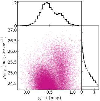
Figure 1: The complete sample of LSBGs from the Y3 DES catalog in color-surface-brightness space is shown along with the histograms along the two axes. Through visual inspection it is apparent that the red and blue LSBGs occupy different loci in this space.

3 Host Galaxy Selection and their Properties

The host galaxies by virtue of their mass exert a dominating influence on the dwarf galaxies around them. Therefore to understand how they quench the nearby LSBG population we begin by carefully selecting a sample based on their mass and environment and then define the boundaries of their halos. We associate LSBGs to them in projection, which makes it necessary to outline the mode of background subtraction that we apply. Here in this section we describe our methods in details.

3.1 Sample

We use the z = 0 Multiwavelength Galaxy Synthesis (z0MGS Leroy et al., 2019) atlas of galaxies in the local universe (distances $D<100$ Mpc) to determine the host sample. This robustly determined catalog is based on ultraviolet, near-infrared, and mid-infrared images from NASA’s Wide-field Infrared Survey Explorer (WISE) and Galaxy Evolution Explorer (GALEX) missions. This catalog contains the stellar mass $\mathcal{M}_{\star}$, star formation rates (SFR) and distance estimates for the galaxies in this work. Their masses cover the LMC to MW mass range we are interested in, making this catalog befitting to use as the host sample in this work.

3.2 Halo Boundary

We define the boundary of the host halo as the virial radius, particularly adopting the definition where this corresponds to the extent within which the density of the halo is 200 times the critical density, $\mathcal{R}_{200}$. For this purpose, we need to calculate the virial mass $M_{200}$ first, which we derive from the stellar masses $\mathcal{M}_{\ast}$ provided in the z0MGS catalog and a stellar-halo mass relation (SHMR) relation. For this purpose we adopt the robust SHMR of Behroozi et al. (2010) that is established through abundance matching. We use the same definition of the halo boundary for the hosts residing in cluster as those in isolated environments.

Having defined the halo boundary, we proceed to define the zones around the halo that will be relevant in this study. Galaxies located at 3D radial distances within $\mathcal{R}_{200}$ are typically considered to be satellite galaxies. The associated population of galaxies we are interested in are located beyond $\mathcal{R}_{200}$ . In this work we follow the prescriptions of Buck et al. (2019); Diemer (2021) and adopt $2.5\mathcal{R}_{200}$ as the outer boundary of the associated region. This limit is appropriate as the properties of the associated galaxies change significantly beyond this extent.

3.3 Host-LSBG association

In order to connect the LSBGs as having interacted with the z0MGS hosts, we require the distance information for the former to match that of the latter. While the distances to the hosts are known, this does not follow for the LSBGs because the dataset we use is based on photometry alone. The classical method of spectroscopically measuring distances (e.g. Geha et al. (2017)) and ascribing satellites, backsplash or infalling galaxies around a host becomes prohibitively expensive in observing time when we focus on the LSBGs among them (e.g., Kadowaki et al., 2021; Goto et al., 2023). The surface brightness fluctuation (SBF) method (Carlsten et al., 2019) has been applied for the purpose of measuring distances to photometry derived catalogs of LSBGs (Carlsten et al., 2019; Casey et al., 2022). However, this method can at best be used to probe distances up to a few Mpc with ground-based observations like the DES (Greco et al., 2021). Given the nature of LSBGs it is time intensive to observe a large sample as well. Therefore, these qualities of our sample render the application of the SBF method unsuitable for this work.

Instead, we use the simple yet commonly used method of associating the LSBGs with the nearest host based on their projected angular separation (van Dokkum et al., 2015; Nierenberg et al., 2011; Wang et al., 2014; van der Burg et al., 2016; Zaritsky et al., 2022; Li et al., 2022). However, this method introduces contamination from background galaxies that needs to be statistically subtracted. We describe this process in the following section.

3.4 Background subtraction

When viewing the distribution of LSBGs associated with hosts in projection on the sky, contamination may arise from what are known as interlopers$-$ galaxies in the foreground or background of the host that appear proximate in projection (Zaritsky, 1992). When estimating the level of this contribution, while doing so “globally" is simpler, this leads to biases arising from the way dark matter structure in the universe has been hierachically formed (White & Rees, 1978) and means that there will be larger numbers of interlopers in and around hosts in high density environments and vice versa. A way to circumvent this is to consider the contamination “locally" (Chen et al., 2006; Wang et al., 2014; Alpaslan & Tinker, 2020; Tinker et al., 2021), wherein the contamination signal is evaluated from annular regions around the hosts in consideration.

In the subsequent analysis, we choose annular regions corresponding to separations of $2.5<\theta/\theta_{200}<4.5$ around the hosts to estimate the projected background density of LSBGs. For a given host, this corresponds to a projected angular area $14\times$ and $2.24\times$ larger than the halo and associated regions. For a constant background density of LSBGs, this implies a $S/N$ of 3.46 and 1.73 respectively. A larger area implies that the background estimate is robust to Poisson fluctuations.

Furthermore, since the z0MGS hosts are selected on the basis of a cut on their projected virial radii $\theta_{200}$, this reduces the background contamination. This is because, given a background density of LSBGs, the number of contaminants would increase with a host subtending a large area on the sky.

3.5 Environment

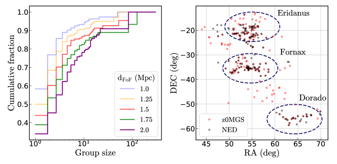
Figure 2: Left: The cumulative fraction of the z0MGS hosts in the DES footprint as a function of their association size for different choices of the linking length $1.0<d_{\rm FoF}<2.0$ Mpc. We choose $d_{\rm FoF}=1.5$ Mpc so that our isolated hosts are robust in terms of their isolation criteria and the clusters hosts are complete in the Fornax region as well. Right: Map of the Fornax region showing the Fornax, Eridanus and Dorado overdensities of galaxies. The red points represent galaxies from the z0MGS catalog making up the four largest FoF groups when using $d_{\rm FoF}=1.5$ Mpc. We compared this with bright galaxies from NED in the same region that have been shown using the gray stars. This shows that our sample of hosts in the cluster environment is complete.

The all-sky z0MGS catalog comprises 15748 members of which 2034 lie within the DES footprint. We employ a Friends Of-Friends (FoF) algorithm to identify regions in the DES footprint with an overdensity of z0MGS galaxies and thereby classify them and the associated LSBGs according to their local environment. FoF algorithms are frequently useful in identifying overdensities in the universe and halo finding in simulations (e.g. Davis et al., 1985; Behroozi et al., 2013). In the context of our work, the FoF algorithm is appropriate in separating out the hosts in the high and low density environments. Compared to works like Yang et al. (2007) which sought to create group catalogs, our application of the FoF algorithm is simpler. For this purpose we utilise the RA, DEC and distance estimates from the host catalog to map out the 3D positions of the galaxies using the astropy.coordinates package. Following this with an appropriately chosen linking length $d_{\rm FoF}$, we identify groups of spatially connected hosts.

Primarily, we want to obtain two samples out of this exercise$-$ a “cluster" sample corresponding to the hosts in the Fornax region and another “isolated" sample which are hosts dwelling in the low-density field. Using Figure 2 we lay out the reasoning behind the value of $d_{\rm FoF}$ used in this work. In the left inset, we plot the cumulative fraction of the z0MGS hosts in the DES footprint as a function of size of the FoF group. The different colored lines show this fraction for various values of $d_{\rm FoF}$ chosen between 1-2 Mpc. This was done to determine the best choice of $d_{\rm FoF}$ with the constraints that this would ensure completeness of the host sample in the Fornax region while keeping the isolated host sample remote from higher density environment. Those FoF groups that were identified as containing single galaxies made up the isolated sample whereas the largest few groups of $\sim 100$ member galaxies were found to be located near the Fornax region. We notice that the primary effect of taking a smaller value of $d_{\rm FoF}$ is to increase the number of isolated hosts and decrease the number of the hosts in the cluster environment. However, we are unable to indefinitely increase the value of $d_{\rm FoF}$ because it tends to an incomplete identification of the cluster hosts.

We attain a balance by taking $d_{\rm FoF}=1.5$ Mpc which is reasonable because it satifies the constraints for both cluster and isolated samples. Out of 2034 galaxies$-$ 195 are in the cluster environment corresponding to the four largest FoF groups, 894 are isolated, and 945 are associated with intermediate sized FoF groups. In the right panel of Figure 2 we show the map of the cluster hosts that we identified using $d_{\rm FoF}=1.5$ Mpc and compare them with member galaxies in the same region obtained from the NASA Extragalactic Database (NED). We find that our cluster sample is reasonably complete around the Fornax, Eridanus and Doradus overdensities and takes into account those galaxies located in the filaments between them. Our choice is consistent with the definition adopted in (Geha et al., 2012; Dickey et al., 2021) wherein galaxies at separations $>1.5$ Mpc are considered isolated. Such a choice of $d_{\rm FoF}=1.5$ Mpc is more conservative than other examples in the literature (e.g. Wang et al. (2014); Brainerd & Samuels (2020)) but it nonetheless enables us to robustly select the sample of isolated hosts.

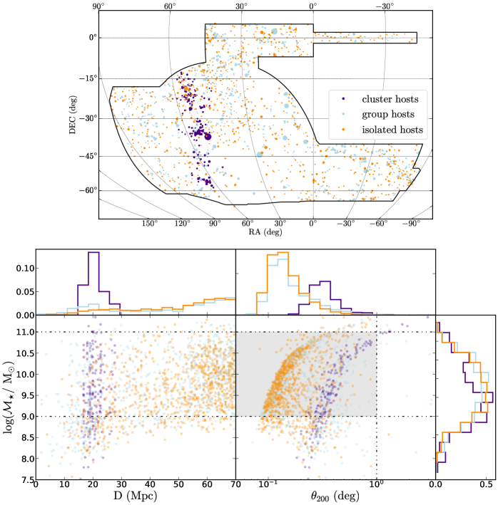
Figure 3: Upper panel: The distribution of z0MGS galaxies in the DES footprint with the colors indigo, light blue and orange depicting those belonging to the cluster, groups and isolated subsamples by the FoF algorithm respectively. The size of each point is proportional to the projected virial radii $\theta_{200}$ of the respective galaxy. Lower left panel: The distribution of these galaxies in $\mathcal{M}_{\star}-D$ stellar mass-distance space. The horizontal dash-dotted lines show the mass cuts that have been adopted in this work $9.0<{\rm log}(\mathcal{M}_{\star}/M_{\odot})<11.0$ with the shaded gray box representing the region of the space from which our sample of hosts are drawn. Lower right panel: The distribution of these galaxies in $\mathcal{M}_{\star}-\theta_{200}$ stellar mass-projected virial radius space. The vertical dash-dotted line is the cut on $\theta_{200}=1.0$ deg that we have adopted here. The histograms show the marginalized distributions for each of the axes.

The respective host samples have been mapped out over the full DES footprint in the upper panel of Fig. 3 whereas the distributions of stellar mass $\mathcal{M}_{\star}$, distance $D$ and projected virial radius $\theta_{200}$ has been plotted in the lower panel of the same. The cluster and the isolated hosts sample have been depicted using indigo and orange colors respectively. Also shown are hosts in intermediate size groups in light blue color although we do not explore their effect on LSBGs further in this work. The cluster hosts in and around Fornax are prominent on the map as well as in the distance histograms. Fornax is the second closest cluster and has been the subject of thorough searches for dwarf galaxies (Caldwell & Bothun, 1987; Ferguson, 1989), with a known presence of a large number of LSBGs (Davies et al., 1988; Caldwell & Bothun, 1987; Muñoz et al., 2015; Venhola et al., 2017). Associated with it is the Eridanus cluster (Gould, 1993; Brough et al., 2006). This association together with Dorado group is part of the larger Southern Supercluster (de Vaucouleurs, 1953; Mitra, 1989) and is identified by the FoF algorithm as a single region. This provides a standard of reference to compare with the LSBGs that dwell in the low density regions of the DES footprint.

These structures together contain the largest number of z0MGS hosts in the footprint and correspondingly an overdensity of LSBGs. In Tanoglidis et al. (2021), while Fornax comes up as two peaks in overdensity associated with Abell S373 located at $18.97\pm 1.33$ Mpc, the Eridanus group is separately designated as the source RXC J0340.1-1835 and is located at a distance of $23.41\pm 1.64$ Mpc (NED).

The z0MGS galaxies that make up the isolated host sample are approximately uniformly distributed across the DES footprint except at the locations of a few voids. Given the criterion for the FoF search used to select these hosts, this means that the nearest massive galaxy is beyond 1.5 Mpc away. This implies that this selection of host galaxies is more isolated in comparision to the MW, M31, M81, IC 342, Maffei 1 and Sculptor in the Local Volume (Karachentsev, 2005).

3.6 Sample cuts

In order to restrict our sample to host galaxies with masses similar to the LMC ($2.7\times 10^{9}M_{\odot}$; van der Marel et al. (2002)) and the Milky Way ($(5.43\pm 0.57)\times 10^{10}M_{\odot}$; McMillan (2017), $(6.08\pm 1.14)\times 10^{10}M_{\odot}$; Licquia & Newman (2015)) we place cuts on the stellar mass such that 10${}^{9}M_{\odot}<\mathcal{M}_{\star}<$ 10${}^{11}M_{\odot}$. We considered using the distance $D$ of these galaxies to restrict the sample of hosts to those situated in the low redshift. The z0MGS sample is incomplete at distances beyond 70 Mpc. Closer by, e.g. within 5 Mpc, the LSBGs are found to be shredded by virtue of the detection pipeline (Tanoglidis et al., 2021).

We instead rely on a cut on the projected virial radius $\theta_{200}$ of the host since reducing the level of background contamination is our main concern. The $\theta_{200}$ is calculated from the host stellar mass using the stellar-halo mass relation (SHMR) in Behroozi et al. (2010) to obtain the physical virial radius projected at the distance $D$. Choosing hosts with a small $\theta_{200}$ lets us mitigate the contamination from foreground/background LSBGs associated with not only nearby hosts projecting a large virial radius but also the distant hosts.

We choose to use an upper limit on the projected virial radius of these hosts $\theta_{200}<1.0$ deg to limit contamination from the background. This limits our sample to 856 host galaxies$-$ 138 in clusters and 718 in isolation. In Fig. 3 we map the host sample selected on the basis of their environment from the z0MGS catalog in the upper panel. We show the distributions in $\mathcal{M}_{\star}-D$ space as well as in $\mathcal{M}_{\star}-\theta_{200}$ space in the lower panels, respectively

Adopting this cut on $\theta_{200}$ can potentially lead to a selection bias against the more massive cluster hosts, as seen in the right panel of Fig. 3. We see that the mode of the $\theta_{200}$ distribution, the cluster hosts have, by virtue of their proximity to us, is larger than the isolated hosts. Therefore imposing the upper limit on $\theta_{200}$ has the result of filtering out a few of the cluster hosts that have $\mathcal{M}_{\star}>10^{10.5}M_{\ast}$.

4 Identification & Characterization of Quenched LSBGs

Having classified the z0MGS hosts according to their environment, we seek to identify and characterize LSBGs around them. We undertake a novel attempt to identify satellite and associated LSBGs around MW and LMC mass isolated hosts and ascertain if quenching has affected them using their color and surface brightness information. The larger goal here being to identify the environmental dependence of the quenching mechanisms$-$ how they might vary between the extremities of cluster and isolated environments. This is a novel investigation of how quenching operates in associated LSBGs. For this purpose we use two distinct yet somewhat parallel methods$-$ the projected surface density profiles around the hosts and the distributions in color surface-brightness (CSB) space.

4.1 Statistical signal of Satellite & Associated galaxies

A way to directly study overdensities of galaxies around massive hosts is to look at their radial distribution through projected surface density profiles (e.g. Nagai & Kravtsov, 2005; van den Bosch et al., 2005; Wang et al., 2014). This motivated Tanoglidis et al. (2021) to look at the radial profiles of LSBGs around density peaks in the DES footprint and which they found are comparable with the radial profiles for bright galaxies in the 2MPZ survey. Using radial profiles, Roberts et al. (in prep.) found overdensities around local universe hosts with LMC and MW masses. We now carry forward this investigation by looking at the projected density profiles of the LSBGs around the more extensive z0MGS host sample.

In order to determine the raw projected density profile, we first find the raw number counts of LSBGs around each host in bins of the angular separation normalized with respect to the projected virial radius, $\theta/\theta_{200}$. The bins cover the range $(0.0,2.5)$. The counts are then normalized with respect to the dimensionless annular area corresponding to the $\theta/\theta_{200}$ of each bin. The choice of using this is motivated by the fact that different hosts have different masses and are situated at different distances, therefore working in dimensionless units enables us to regularize these host-to-host variations. We determine the background contribution to the density profile for each host by selecting an annulus with $2.5<\theta/\theta_{200}<4.5$ and finding the average density of LSBGs in it. We subtract the background density from the raw projected density profile to determine the projected density profile $\Sigma(\theta/\theta_{200})$. We then stack these profiles and calculate the mean and the standard deviation using the bootstrap method wherein we sample among the hosts in 5000 iterations. The standard error on the mean is derived by appropriately normalizing by the square-root of the total number of hosts.

In Figure 4 we plot the density profiles $\Sigma(\theta/\theta_{200})$ according the environment of the z0MGS host. The dashed lines show the level of background density that was subtracted to obtain the profiles. All the shaded regions signify the standard error from the bootstrap method. The extent of the profile for $\theta/\theta_{200}<1$ and $1<\theta/\theta_{200}<2.5$ correspond to the satellite and associated populations, respectively. Since there is possible incompleteness at small radial distances due to blending with the host galaxy (van der Burg et al., 2016; Li et al., 2023) we highlight a conservative approximation of this domain at $\theta/\theta_{200}<0.25$ to show where this effect might be prominent. We performed a visual inspection and found blending effects were limited within this region.

Since we are interested in the clustering of LSBGs around z0MGS hosts with stellar masses in the range of the LMC and MW, we separate the host sample into two bins of $9.0<{\rm log}(\mathcal{M}_{\star}/M_{\odot})<10.0$ and $10.0<{\rm log}(\mathcal{M}_{\star}/M_{\odot})<11.0$ roughly corresponding to the measured stellar mass of each of the objects (van der Marel et al., 2002; McMillan, 2017). The corresponding profiles are depicted using the pink and blue colored lines in Figure 4 with the left and right panels depicting the profiles around hosts in the cluster and isolated environments respectively. We find that the radial profiles in the two mass bins closely resemble each other in both environments with a notable concentration of LSBGs inside the virial radius ($\theta/\theta_{200}<1$). However there is an enhancement in normalization of the profiles as well as the background level for the cluster hosts compared to the isolated hosts which is expected given the high density environment of the former sample.

We tested the statistical significance of our result by comparing the raw number of satellite and associated LSBGs $N_{\rm LSBG}(\theta/\theta_{200})$ with that of mock background LSBGs in the different bins of $\theta/\theta_{200}$. For this we took the projected background density from $2.5<\theta/\theta_{200}<4.5$ and obtained the expected number of mock LSBGs for each annuli of $\theta/\theta_{200}$. This is used as a parameter for a Poisson distribution from which we sample the mock number of LSBGs $N_{\rm mock}(\theta/\theta_{200})$. We calculated 10000 realizations and none produced more counts of $N_{\rm mock}(\theta/\theta_{200})$ than the measured $N_{\rm LSBG}(\theta/\theta_{200})$ except the largest radial bin for LMC analogous hosts in the isolated environment. In those cases the fraction of realizations where the mocks exceeded the measured count was $\sim 0.0012$. This shows that the detection of the overdensities of satellite and associated LSBGs near the z0MGS hosts is robust against contamination from the background.

The phenomena we notice here, when the profiles are differentiated by the host properties, is essentially representative of the same result of hierarchical structure formation (White & Frenk, 1991). This is namely that massive halos and halos in denser regions collapse earlier, leading to richer substructure around the central galaxies harbored in them. Furthermore, the profiles smoothly decay beyond the virial radii of the hosts where the associated LSBGs are located. This shows that the quenching does not simply end at the virial radius and may continue beyond it, thus highlighting the presence of backsplash and infalling LSBGs around these hosts (Ludlow et al., 2009).

We similarly obtain the background subtracted density profiles around hosts analogous to the MW in the mass bin $10.0<{\rm log}(\mathcal{M}_{\star}/M_{\odot})<11.0$, but this time we separate out the LSBGs by their $g-i$ and $\mu_{\rm eff,g}$ values. These profiles are shown in the upper and lower rows of panels in Fig. 5 with the left and right columns showing the profiles around the cluster and isolated hosts, respectively. The LSBGs are separated into a "red" and "blue" populations by their $g-i$ color with a fiducial threshold value of 0.6 mag (Tanoglidis et al., 2021). When separating by their $\mu_{\rm eff,g}$ values into bright and faint populations, we use a threshold of $25.7\,\rm{mag\,arcsec}^{-2}$, which is the mean value of the surface brightness cuts that we employed (see Sec 2).

We find that across both environments the profiles of red LSBGs ($g-i>0.6$) have a higher concentration within the virial radius ($\theta/\theta_{200}<1$) relative to the background level. This occurs with an overall difference in normalization even beyond $\theta/\theta_{200}<1$ with respect to the profiles of its blue ($g-i<0.6$) counterparts. The profiles for the cluster hosts are flatter and the background levels are also larger, especially for the red LSBGs. The profiles for the bright LSBGs ($\mu_{\rm eff,g}>25.7\,\rm{mag\,arcsec}^{-2}$) show a significant overdensity for $\theta/\theta_{200}<1$, although they are lower in normalization compared to the fainter counterparts ($\mu_{\rm eff,g}<25.7\,\rm{mag\,arcsec}^{-2}$) in both types of host environments.

The presence of an overdensity of red LSBGs around these hosts is a signature of quenching of LSBGs taking place in the respective environments (Karunakaran et al., 2022). Noticeably, this is present in hosts in the clusters who themselves make up the substructure of the more massive cluster host as well as the isolated hosts in the low density environment. This shows the ubiquity of MW-like hosts ($10.0<{\rm log}(\mathcal{M}_{\star}/M_{\odot})<11.0$) in shaping LSBG evolution across diverse environments. In order to probe this further we consider the color-surface brightness distributions of satellites and associates separately in the next section.

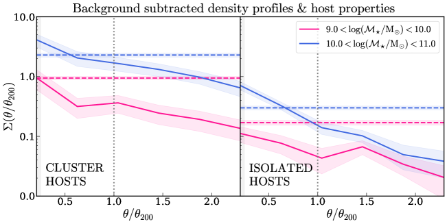
Figure 4: The background subtracted projected surface density profile $\Sigma(\theta/\theta_{200})$ of LSBGs around z0MGS hosts belonging to cluster (left panel) and isolated environments (right panel) with LMC like stellar masses $9.0<{\rm log}(\mathcal{M}_{\star}/M_{\odot})<10.0$ (pink line) and MW-like masses ($10.0<{\rm log}(\mathcal{M}_{\star}/M_{\odot})<11.0$) (blue line). The dashed horizontal lines show the average density of LSBGs at separations of $2.5<\theta/\theta_{200}<4.5$ from the respective sample of hosts, which constitute a measurement of the background level. The colored shaded regions show the uncertainties on the $\Sigma(\theta/\theta_{200})$ estimated using the bootstrap method. The dotted black line is $\theta/\theta_{200}=1$ represents the extent of the typical virial radii of the hosts. The gray shaded region at $\theta/\theta_{200}<0.25$ shows the region where incompleteness of the LSBG sample might arise due to blending with the host galaxies.

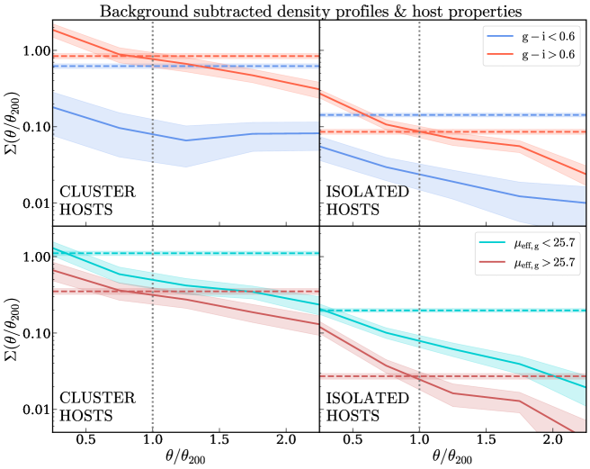
Figure 5: The background subtracted projected surface density profile $\Sigma(\theta/\theta_{200})$ of LSBGs around the z0MGS hosts belonging to cluster (left column) and isolated environments (right column) separated by the $g-i$ color of the LSBGs (upper row) and by their surface brightness $\mu_{\rm eff,g}$ (lower row). The dashed horizontal lines show the average density of LSBGs at separations of $2.5<\theta/\theta_{200}<4.5$, which constitute a measurement of the background level. The colored, shaded regions show the uncertainties on $\Sigma(\theta/\theta_{200})$ estimated using the bootstrap method. The dotted black line is $\theta/\theta_{200}=1$ represents the extent of the typical virial radii of the hosts. The gray shaded region at $\theta/\theta_{200}<0.25$ shows the region where incompleteness of the LSBG sample might arise due to blending with the host galaxies.

4.2 Hess diagrams in Color$-$ Surface Brightness space

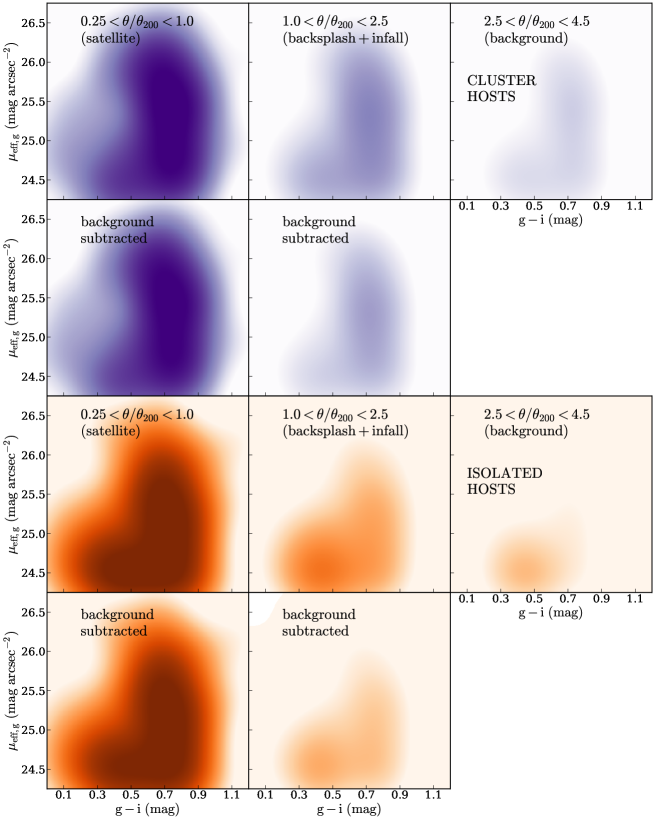
Figure 6: The maps of Kernel Density Estimates (KDE) in the color-surface brightness (CSB) space of LSBGs around hosts with $9.0<{\rm log}(\mathcal{M}_{\star}/M_{\odot})<11.0$ belonging to the environments of clusters (top two rows, blue) and in isolation (bottom two rows, orange) and at different bins of angular separations $\theta$. The bins with $\theta/\theta_{200}<1$ (left) and $1<\theta/\theta_{200}<2.5$ (center) corresponds to populations of satellites and associated galaxies (backsplash+infalling), respectively, whereas the outer bin KDE with $2.5<\theta/\theta_{200}<4.5$ (right, first and third rows) constitutes the basis for measuring the background contamination. The background subtracted KDE (second and fourth rows) reveals a distinct red sequence visible for the satellites LSBGs in both cluster and isolated environments while the associated LSBGs in the latter show a less prominent red sequence and an enhanced blue cloud. These are the patterns of quenching taking place in the respective environments, while the associated LSBGs in the low density environment, are seemingly still undergoing the process of quenching.

We seek to explore the relationship between the photometric and spatial clustering properties further. Here we revisit the color-surface brightness (CSB) distribution of the LSBGs shown in Figure 1. However with the insight gained from Section 4.1, we look to incorporate the spatial density of these objects in their CSB distributions. Working with spatial densities as opposed to using raw counts, enables us to subtract the background contribution from the signal of interest in the CSB space.

For this purpose, the we employ the concept of a Hess diagram. Historically, they have been used to depict the spatial density of stars across regions of color-magnitude space to study globular clusters and dwarf galaxies (Hess, 1924; Gaposchkin, 1948). Although those studies focused on resolved stellar populations and especially the identification of the main sequence, it is essentially parallel to our investigation of the red sequence of quenched LSBGs in the CSB space. We start by determining the probability density of LSBGs in the CSB space. Instead of working with densities computed on discrete 2D bins, we choose the smoothness and continuity of distributions that is guaranteed by using a Kernel Density Estimator (KDE). A Gaussian kernel with bandwidth of 0.1 is used for the KDE, after having renormalized the parameters to the interval $(0,1)$. We ensure that the bandwidth is larger than the typical uncertainty of a point in the CSB space. On the other hand, making the bandwidth arbitrarily large can dissolve features in the CSB distribution.

We show the KDE for the LSBGs in different environments using the Hess diagrams in Fig. 6. The upper half correspond to the cluster and the lower half the isolated environments. For each of these hosts we look at nearby LSBGs and then split their population according to their projected separation from the host $\theta$ normalized by the projected virial radius of the host $\theta_{200}$. Three regions are $\theta/\theta_{200}<1$ for the satellites, $1<\theta/\theta_{200}<2.5$ for the associated galaxies and we use $2.5<\theta/\theta_{200}<4.5$ to estimate the contamination from background objects. The KDEs corresponding to these three regions are displayed in the three columns from left to right. We normalize the KDE with the total angular region of the footprint as considered in each bin. We then subtract the background KDE from the target KDE to give us the KDE shown in the right column.

Fig. 6 shows the background subtracted KDEs for the satellite and associated LSBGs across the two environments, with the darker regions representing a higher density of LSBGs at a given $g-i$ and $\mu_{\rm eff,g}$. The distributions belonging to the satellite and associated regions in the cluster environment show a distinct red sequence at $g-i>0.6$ stretching across $24.5<\mu_{\rm eff,g}<26.5\,\rm{mag\,arcsec}^{-2}$ in both the satellite and associated regions. The distributions near the isolated hosts also show prominent red sequences for both regions. However it is at $\mu_{\rm eff,g}<25.0\,\rm{mag\,arcsec}^{-2}$ where the distributions show an interesting deviation between the environments. We notice an enhanced blue cloud around $0.1<g-i<0.4$ in contrast to the cluster distribution. There is also an enhancement across $0.4<g-i<0.6$ between the two features that is the green valley (Kauffmann et al., 2003).

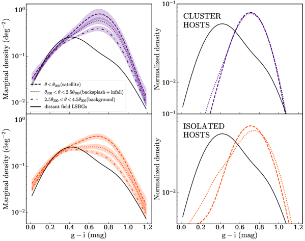
Figure 7: Left: The marginalized KDEs as functions of $g-i$ are shown for the satellite ($0.25<\theta/\theta_{200}<1$), the associated ($1<\theta/\theta_{200}<2.5$) as well as the background ($2.5<\theta/\theta_{200}<4.5$) LSBGs as the dashed, dotted, and dash-dotted lines respectively. The cluster and isolated environments of the LSBGs are coded using blue and orange colors respectively. The black histogram is that of the distant field sample not within $2.5\theta/\theta_{200}$ of a z0MGS host in the footprint. Right: The marginalized KDEs for the satellite and associated from which the background has been subtracted and re-normalized so that the areas under the curves are equal to one. All the color distributions of the satellite and associated galaxies deviate significantly from that of the field sample. They peak at $g-i=0.72$ where there is a notable red excess with respect to the distant field value. This shows that the LSBGs are being quenched by virtue of their environment, near the z0MGS hosts, rather than intrinsic reasons.

4.3 Marginalized Color distributions

To shed more light on the detection of the red sequence, we marginalize these distributions over the surface brightness axis to yield the $g-i$ color distributions for the LSBGs in the various regions and compare with the color distribution for a field sample of LSBGs. This lets us explore the color bimodality aspect of the LSBG distributions as seen in Fig. 1. We plot these distributions in the left panel of Fig. 7 with the right panel showing the same distributions with background subtraction and normalization such that the area under the curves equals to the average number density of the respective sample. We depict both the satellite ($\theta/\theta_{200}<1$) as well as the associated ($1<\theta/\theta_{200}<2.5$) populations as the dashed and dotted lines respectively. The shaded regions represents the uncertainties that have been determined through bootstrap resampling. The dash-dotted line in the left panel show the background ($2.5<\theta/\theta_{200}<4.5$) distributions which is subtracted from the satellite and associated distributions. While the simple marginalized distributions on the left show the number densities of each LSBG population, the normalized distributions on the right enables us to compare their shapes.

The KDE for the $g-i$ distribution of the “distant field" LSBG sample is shown as the black solid line. This sample is conservatively selected by ensuring that these LSBGs are not within 2.5$\theta_{200}$ of any z0MGS galaxy. To mitigate boundary effects we take into account the z0MGS members beyond the footprint as well during the process of selection. The equivalent area in the footprint that is not within 2.5$\theta_{200}$ of any z0MGS galaxy is 1565 deg² which we determined using a Monte Carlo method. The way the distant field sample is selected ensures that these LSBGs are situated in voids at low redshifts. In the latter case, we expect massive, luminous LSBGs to dominate unlike the faint, small LSBGs found near us (Tanoglidis et al., 2021).

We find that all of the LSBGs distributions in the cluster environment show broad peaks with a heavy tail towards the blue side. The distributions peak at $g-i=0.72$. Concerning the LSBGs around the isolated hosts, we find that the peaks of the distributions are significantly more broad. While the satellites have a peak in the distribution close to where the cluster LSBGs peak, the associated LSBGs are more skewed. We find a difference between the satellites and associated LSBGs in both environments from the very blue tail of the distribution $g-i\gtrsim 0.0$. In contrast, the red tails at $g-i\gtrsim 1.0$ show similarity for the two populations in both cases. The distribution of these field LSBGs by inspection is bluer than that for the LSBGs near the z0MGS hosts. All the LSBG distributions show a significant excess near their peaks at $g-i=0.72$ with respect to the field distribution. There is also a notable difference at the red and the blue ends of the distribution except for the case of associated LSBGs of isolated hosts showing a convergence at $g-i\gtrsim 0.4$.

We apply the two sample 1-D Kolmogorov–Smirnov test (K-S test) to test the dissimilarity of the different distributions. Comparing the distributions for the satellite and associated populations, we find a p-value that is $<0.01\%$ in both the cluster and isolated environments. We can therefore reject the null hypothesis that the satellite and associated populations are drawn from the same distribution. It is also interesting to compare these distributions with the field population of LSBGs. We find from the p-value which is $<0.01\%$ that the LSBG populations of satellites and associates near the z0MGS hosts show $g-i$ distributions distinct from each other as well as those selected from out in the field.

5 Discussion

In this work, we measure and characterize LSBG populations in the cluster and isolated environments they are embedded in. We place our key findings from Sec. 4 in context of the contemporary understanding of the field. Our findings can be summarized as follows: 1. We detect an overdensity of red and bright LSBGs in the radial density profiles near z0MGS hosts with a wide range of masses that are situated in both dense and sparse environments in Sec 4.1. 2. We identify a red sequence of LSBGs in their color-surface brightness (CSB) space in Sec 4.2. 3. We find a red-excess with respect to the distant field population in the $g-i$ color distribution of 4.3. These are statistical detections made after correcting for background subtraction and point towards the host galaxies influencing the properties of the LSBGs beyond their virial radius. These results direct us to explore the importance of the connection between hosts and both backsplash and infalling galaxies in Sec. 5.1. Then in Sec. 5.2 we touch upon the theme of environmental quenching like pre-processing in low density environments that is an effect of this connection.

5.1 Backsplash & Infalling Galaxies

Outside the virial radius of a central galaxy, there exists a heterogeneous population of lower mass galaxies. This includes backsplash galaxies which have already completed pericentric passages as well as those on their first infall into the central. The former are expected to be quenched as result of the pericentric passage and to appear as older, redder stellar populations relative to the infalling galaxies and those in the field (Wetzel et al., 2014; Simpson et al., 2018; Ferreras et al., 2023). Echoing Ludlow et al. (2009), we collectively call these galaxies which are located at projected separations of $\theta_{200}<\theta<2.5\theta_{200}$, associated galaxies. The existence of such galaxies show that the spheres of influence of massive centrals extend far beyond their virial radii (e.g. Bahé et al., 2013; Behroozi et al., 2014). Using simulations Bakels et al. (2021) and Borrow et al. (2022) show that out of all the associated galaxies beyond the virial radii of MW-like hosts, the fraction of backsplash galaxies is $\approx 50\%$ between $1-1.2\mathcal{R}_{200}$. The ubiquitousness of these galaxies is pointed out by their presence in a diverse range of environment (Balogh et al., 2000; Wang et al., 2009; Simpson et al., 2018). For example, the Tucana and Cetus galaxies (Sales et al., 2007; Teyssier et al., 2012; Santos-Santos et al., 2022) are dwarf backsplash candidates around the Local Group.

LSBGs are known to constitute a sizeable subset of the low mass galaxies in the vicinity of MW and LMC mass hosts in the Local Volume (Karachentsev & Kaisina, 2022), including those hosts in isolated environments. LSBGs which are on backsplash and infalling orbits around massive central have been observed in simulations (e.g. Applebaum et al., 2021), with backsplash galaxies occasionally found as far as $\approx 5\mathcal{R}_{200}$ from the more massive central (Teyssier et al., 2012; Benavides et al., 2021). In this work we not only detect LSBG populations around z0MGS hosts across different environments, including those with LMC like masses, we demonstrate that the population of red LSBGs extends to at least $2.5\times$ the projected virial radius. These populations are characterized by their relative redness and low surface brightness with respect to LSBGs in the field and indicate they have interacted with the hosts during the course of their backsplash or infall orbits. Our detection of red LSBGs around MW and LMC analogous hosts therefore establishes that LSBGs which also happen to be associated galaxies constitute an important component of the substructure of these hosts.

Our findings highlight the importance of accounting for galaxies at the intersection of LSBGs and associated galaxies in order to gain a complete understanding of the outer extents of the halos of MW and LMC mass galaxies in isolated, group and cluster environments. There have already been challenges to the classical “spherical overdensity” based classical definition of the virial radius with the “splashback” definition (Diemer & Kravtsov, 2014; Adhikari et al., 2014; More et al., 2015). The latter represents the extent of dark matter material at their first apocenter around the host and also changes how we look at subhalos around the hosts (Diemer, 2021). For example, if we defined the halo boundary by the splashback radius rather than the viral radius the associated galaxies considered in this work would now be classified as satellites instead. When galaxies around cluster mass hosts are selected according to their colors and their splashback radius measured from their density profiles (Baxter et al., 2017; Adhikari et al., 2021), it is seen that red galaxies have been in the cluster longer compared to the blue galaxies. While the splashback radii of cluster scale systems have been studied extensively (More et al., 2016), the presence of associated galaxies enable a novel method to probe not only the splashback radii but the structure and composition of the outer halo beyond the virial radius of group scale or isolated systems.

In such associated galaxies, we get a better understanding if their HI gas distribution that is susceptible to removal through ram-pressure stripping (Simpson et al., 2018) can be traced. Dwarf galaxies within the Local Group are known to be deficient in their HI content (Teyssier et al., 2012; Putman et al., 2021). Ever though it is difficult to constrain the HI content of LSBGs given current instrumental sensitivities (Zhou et al., 2022), there is promise for the future with the upcoming WALLABY (Koribalski et al., 2020) and SKA (Dewdney et al., 2009) radio surveys.

On the other hand optical photometry alone is not fruitful either in separating the populations of associated galaxies because there are degeneracies between the observables of quenching between backsplash orbits and pre-processing of the infalling satellites (Knebe et al., 2011). In the Local Group, availability of proper motion measurements (McConnachie et al., 2021; Battaglia et al., 2022) enables us to determine backsplash candidates. Beyond the Local Group, measuring distances using the surface brightness fluctuation (SBF) method has lead to the detection of a backsplash LSBG in Casey et al. (2022) with $\mu_{\rm eff,R}=24.71\,\rm{mag\,arcsec}^{-2}$, $r_{\rm eff}=0.79$ kpc) that is associated with the M81 galaxy as its host. Named dw0910p7326 this galaxy is apparently composed of a quenched old stellar population with an age of $\lesssim 10$ Gyr. Particularly, LSST is poised to improve SBF based distance measurements with higher quality of data within the first few years of its survey (Greco et al., 2021). Tidal removal of dark matter from the outskirts of backsplash LSBGs can also lead to an increase in their subhalo-stellar mass ratio of these objects. Stacking the dark matter density profiles derived from weak lensing (Sifón et al., 2018) is another way to study the orbital histories of the associated LSBGs in a better fashion.

5.2 Quenching

The presence of the red-excess in the $g-i{}$ color distributions for the both the satellite and associated LSBGs around cluster and isolated hosts of MW and LMC masses shows the evidence of environmental quenching (e.g. Fillingham et al., 2018) processing of the LSBGs. The method of background subtraction and consequent comparison with the distant field sample furthermore rules out the role of internal mechanisms of quenching like stellar feedback or reionization (Di Cintio et al., 2017; Hayward & Hopkins, 2017). While LSBGs in dense cluster environments are known to be red (van Dokkum et al., 2015; van der Burg et al., 2016; Bachmann et al., 2021; Zaritsky et al., 2022) with similar processes of quenching have acted on them as those on higher surface brightness galaxies. On the other hand, LSBGs in the field have been observed to be star-forming (Leisman et al., 2017) with only $26\pm 5$ per cent of isolated LSBGs being quiescent (Prole et al., 2021).

To understand the quenching of LSBGs, we also need to know how this is connected to their low surface-brightness nature. Li et al. (2023) found that the quenched fraction of satellite LSBGs around MW analogs matches that of the broader sample of classical dwarfs (Carlsten et al., 2022a). Therefore, the diffuse nature of LSBGs can be explained as some process that “puffs up" hitherto normal sized dwarfs (Li et al., 2023) causing a vertical movement in the mass-size space at fixed stellar mass. This on top of any reduction in luminosity caused due to quenching, should increase the effective surface brightness (which depends on galaxy size and luminosity). Therefore this process should produce a shift in $\mu_{\rm eff,g}$ towards the faint end of the CSB space. Simulations show that this can arise from an internal mechanism like supernovae feedback (Di Cintio et al., 2017) or environmental processes like tidal heating and ram-pressure stripping (Jiang et al., 2019). Antlia 2, Crater 2 (Torrealba et al., 2016, 2019; Ji et al., 2021) AndXIX, AndXXI, AndXXIII (Martin et al., 2016; Collins et al., 2020, 2021), Scl-MM-Dw2 (Mutlu-Pakdil et al., 2022), and NGC 55-dw1 (McNanna et al., 2023) are examples of recently discovered faint, diffuse satellites whose nature can be attributed to intense tidal stripping by their hosts. Furthermore, Sales et al. (2020) and Benavides et al. (2022) show that among the population of satellite UDGs in the group environment, a fraction were field UDGs before infall while the rest became UDGs after infall aided by tidal heating in the host environment. At the same time there might be multiple mechanisms shaping these objects over the course of their lifetimes (Papastergis et al., 2017). According to Kado-Fong et al. (2021) the shapes of LSBGs are a means to distinguish between the various formation theories that is independent of the LSBG environment.

The same processes are known to lead to quenching as well. While tidal heating plays a role in quenching, the effect of ram-pressure stripping becomes stronger with a higher ambient density (Martin et al., 2019). Accordingly, greater ram-pressure stripping is expected to take place closer to the center of the host halo where the density is high. This is the plausible reason for the increase in the quiescent fraction in bright galaxies (Sales et al., 2015; Karunakaran et al., 2022) and LSBGs alike (Greene et al., 2022a; Karunakaran & Zaritsky, 2022). The properties of the infalling galaxy also determines the future state of star formation as more massive systems are more resilient to the quenching processes (Pan et al., 2022; Benavides et al., 2022). Quenching should correspond to a horizontal movement of galaxies from bluer to redder values of $g-i$ in the CSB space.

The sample of LSBGs inside the Fornax-Eridanus cluster provide the best way to probe these processes in depth. The projected radial distributions show that they are bound to the z0MGS hosts in the same environment. This results in what is known as galactic conformity (Weinmann et al., 2006) where red dwarfs cluster strongly with respect to the red hosts. The z0MGS hosts that are in the cluster have been inside this environment longer, implying the satellite and associated LSBGs are also old and quenched. However the same LSBGs also show the effects of being part of the larger cluster scale host as well and thereby shaped by the intercluster medium (ICM). This leads to the radial distributions of cluster LSBGs selected by color being relatively flat and the $g-i$ color distributions of the satellite and associated LSBGs in the cluster environment resembling each other closely. We are interested in seeing how galaxies at different mass scales interact amongst themselves. Since galaxies assemble in the mode of hierachical structure formation, it is likely that their quenching takes place along similar lines. This phenomenon of “hierachical quenching" can be investigated further using low mass cluster substructure (Wang et al., 2023) like the satellite and associated LSBGs we find in this work.

Beyond the extent of the virial radius of the host galaxy, the same processes that contributes to the quenching of satellites acts to deplete the gas reservoirs of infalling dwarfs. For example, the effect of tidal interactions might extend beyond the virial radius as well (Higgs & McConnachie, 2021). Pre-processing involves a population of dwarfs being subjected to ram-pressure stripping within a low-mass group (Roberts & Parker, 2017) followed by their collective accretion on to a MW host (Samuel et al., 2022a, b). The LMC can be held responsible for bringing with it its own population of dwarf galaxies that eventually merged with those of the MW (Deason et al., 2015; Nadler et al., 2020; Patel et al., 2020; Erkal & Belokurov, 2020; D’Souza & Bell, 2021; Jahn et al., 2022; Pace et al., 2022). For example, the backsplash LSBG dw0910p7326 interacted with M81 recently ($\sim 1.5$ Gyr ago) compared to the age of its stellar population suggesting that pre-processing played a role in quenching it (Casey et al., 2022). Alternative mechanisms of environmental quenching of dwarf galaxies include quenching in cosmic sheets (Pasha et al., 2022) and in infall region of galaxy clusters, particularly along filaments (Martínez et al., 2016; Salerno et al., 2022). On the other hand, mergers not only quench galaxy populations but can lead to their diffuse appearances (Wright et al., 2021; Pallero et al., 2022).

Such processes are better investigated around the isolated hosts because they are the highest mass structure in their vicinity. Unlike the cluster LSBGs, we find differences in the properties of the satellite and associated samples namely sharper gradients in their density profile as well as distinct color distributions. Again in line with galactic conformity, these systems are younger and have been assembled recently (Hahn et al., 2007), therefore the LSBGs contained in them have not been well processed like their counterparts inside the cluster. Around these hosts, it is likely that the red sequence/red-excess we are detecting comprises backsplash LSBGs which have properties similar to the satellite LSBGs while the blue cloud and green valley is made up of the infalling LSBGs subject to pre-processing. Nonetheless, such systems will be ideal to probe those mechanisms of environmental quenching disucssed hitherto that can operate beyond the virial radii of the host galaxies.

6 Conclusion

In this work we utilize the full catalog of LSBGs from the Y3 DES catalog, seeking to identify their associations with host galaxies having $9.0<{\rm log}(\mathcal{M}_{\star}/M_{\odot})<11.0$ drawn from the low redshift z0MGS sample. The host sample is sub-divided into cluster and isolated environments based on a Friends Of-Friends algorithm with a linking length of 1.5 Mpc. We use the projected virial radius $\theta_{200}$ to define the boundary of the halo containing the host galaxy and select surrounding LSBGs in terms of its projected separations from the hosts. These galaxies are divided into three bins of projected separation from the hosts: $\theta<\theta_{200}$, $\theta_{200}<\theta<2.5\theta_{200}$ and $2.5\theta_{200}<\theta<4.5\theta_{200}$ that we refer to as the satellite, associated and background samples respectively. Our results are as follows:

• Computing the background subtracted radial density profile, we find that the LSBGs strongly cluster around the z0MGS host galaxies, and this tendency is enhanced around the hosts with MW-like masses and/or in cluster like environments. Redder and brighter LSBGs are more centrally concentrated around the z0MGS hosts relative to the shallower radial profile of the bluer, brighter LSBGs.

• We then use a Kernel Density Estimate of the LSBG samples to construct the equivalent Hess diagrams in color-surface brightness space. After background subtraction, there are well-defined red sequences in both the satellite ($\theta<\theta_{200}$) and associated ($\theta_{200}<\theta<2.5\theta_{200}$) regions in both cluster and isolated environments. The latter environment shows pronounced blue cloud and green valley features that suggest ongoing pre-processing.

• We marginalize these densities along $\mu_{\rm eff,g}$ to generated $g-i$ color distributions of the samples and compare with a distant field sample of LSBGs$-$ not located within $2.5\theta_{200}$ of any z0MGS hosts. There is a clear excess of LSBGs at $g-i\sim 0.7$ with respect to the distant field, as substantiated by comparing using a KS-test.

• These results in combination provide strong support for the existence of quenching in backsplash and infalling LSBGs beyond the classical halo boundary $\theta_{200}$ of the host galaxies. This shows ubiquity of backsplash galaxies across both the environments as well as the importance of pre-processing of infalling galaxies.

Our work casts light on the value of low mass LSBGs in tracing how the environment impacts galaxy evolution of the underlying structure. We see similar quenching signatures in both environments which also shows that the centrals with $9.0<{\rm log}(\mathcal{M}_{\star}/M_{\odot})<11.0$ (Jahn et al., 2022) play an important role in quenching/processing the LSBGs around them.

Investigating systems of either mass scale in the Local Universe beyond the Local Group could herald new discoveries in the field of near-field cosmology. The Legacy Survey of Space and Time (LSST) (Ivezić et al., 2019), promises to push the current detection limits to even lower surface brightness and greater distance, with a great potential of discovery of LSBG systems in the Local Volume Mutlu-Pakdil et al. (2021). Spectroscopic observations can be useful too, e.g., Dragonfly Spectral Line Mapper (Lokhorst et al., 2022) in gaining velocity information that can be used to discern between backsplash and infalling systems. One of the most promising endeavors will be to study the low mass systems using weak lensing in the Merian Survey (Luo et al., 2023).

Author Affiliations

¹ Department of Astronomy, The Ohio State University, Columbus, OH 43210, USA
² Center for Cosmology and Astro-Particle Physics, The Ohio State University, Columbus, OH 43210, USA
³ Department of Physics, The Ohio State University, Columbus, OH 43210, USA
⁴ Institute for Advanced Study, 1 Einstein Drive, Princeton, NJ 08540, USA
⁵ Dartmouth College, Department of Physics and Astronomy, Hanover, NH 03755, USA
⁶ Department of Astronomy and Astrophysics, University of Chicago, Chicago, IL 60637, USA
⁷ Kavli Institute for Cosmological Physics, University of Chicago, Chicago, IL 60637, USA
⁸ Fermi National Accelerator Laboratory, P.O. Box 500, Batavia, IL 60510, USA
⁹ McWilliams Center for Cosmology, Carnegie Mellon University, 5000 Forbes Ave, Pittsburgh, PA 15213, USA
¹⁰ Texas A&M University, College Station, TX 77843, USA
¹¹ Centre for Extragalactic Astronomy, Durham University, South Road, Durham DH1 3LE, UK
¹² Laboratório Interinstitucional de e-Astronomia - LIneA, Rua Gal. José Cristino 77, Rio de Janeiro, RJ - 20921-400, Brazil
¹³ Department of Physics, University of Michigan, Ann Arbor, MI 48109, USA
¹⁴ Institute of Cosmology and Gravitation, University of Portsmouth, Portsmouth, PO1 3FX, UK
¹⁵ Department of Physics & Astronomy, University College London, Gower Street, London, WC1E 6BT, UK
¹⁶ Instituto de Astrofisica de Canarias, E-38205 La Laguna, Tenerife, Spain
¹⁷ Universidad de La Laguna, Dpto. Astrofísica, E-38206 La Laguna, Tenerife, Spain
¹⁸ Institut de Física d’Altes Energies (IFAE), The Barcelona Institute of Science and Technology, Campus UAB, 08193 Bellaterra (Barcelona) Spain
¹⁹ Hamburger Sternwarte, Universität Hamburg, Gojenbergsweg 112, 21029 Hamburg, Germany
²⁰ School of Mathematics and Physics, University of Queensland, Brisbane, QLD 4072, Australia
²¹ Department of Physics, IIT Hyderabad, Kandi, Telangana 502285, India
²² Institute of Theoretical Astrophysics, University of Oslo. P.O. Box 1029 Blindern, NO-0315 Oslo, Norway
²³ Fermi National Accelerator Laboratory, P. O. Box 500, Batavia, IL 60510, USA
²⁴ Instituto de Fisica Teorica UAM/CSIC, Universidad Autonoma de Madrid, 28049 Madrid, Spain
²⁵ University Observatory, Faculty of Physics, Ludwig-Maximilians-Universität, Scheinerstr. 1, 81679 Munich, Germany
²⁶ Center for Astrophysical Surveys, National Center for Supercomputing Applications, 1205 West Clark St., Urbana, IL 61801, USA
²⁷ Department of Astronomy, University of Illinois at Urbana-Champaign, 1002 W. Green Street, Urbana, IL 61801, USA
²⁸ Santa Cruz Institute for Particle Physics, Santa Cruz, CA 95064, USA
²⁹ Center for Astrophysics $|$ Harvard & Smithsonian, 60 Garden Street, Cambridge, MA 02138, USA
³⁰ Australian Astronomical Optics, Macquarie University, North Ryde, NSW 2113, Australia
³¹ Lowell Observatory, 1400 Mars Hill Rd, Flagstaff, AZ 86001, USA
³² George P. and Cynthia Woods Mitchell Institute for Fundamental Physics and Astronomy, and Department of Physics and Astronomy, Texas A&M University, College Station, TX 77843, USA
³³ LPSC Grenoble - 53, Avenue des Martyrs 38026 Grenoble, France
³⁴ Institució Catalana de Recerca i Estudis Avançats, E-08010 Barcelona, Spain
³⁵ Department of Physics, Carnegie Mellon University, Pittsburgh, Pennsylvania 15312, USA
³⁶ Observatório Nacional, Rua Gal. José Cristino 77, Rio de Janeiro, RJ - 20921-400, Brazil
³⁷ Kavli Institute for Particle Astrophysics & Cosmology, P. O. Box 2450, Stanford University, Stanford, CA 94305, USA
³⁸ SLAC National Accelerator Laboratory, Menlo Park, CA 94025, USA
³⁹ Centro de Investigaciones Energéticas, Medioambientales y Tecnológicas (CIEMAT), Madrid, Spain
⁴⁰ Instituto de Física, UFRGS, Caixa Postal 15051, Porto Alegre, RS - 91501-970, Brazil
⁴¹ School of Physics and Astronomy, University of Southampton, Southampton, SO17 1BJ, UK
⁴² Computer Science and Mathematics Division, Oak Ridge National Laboratory, Oak Ridge, TN 37831
⁴³ Cerro Tololo Inter-American Observatory, NSF’s National Optical-Infrared Astronomy Research Laboratory, Casilla 603, La Serena, Chile
⁴⁴ Lawrence Berkeley National Laboratory, 1 Cyclotron Road, Berkeley, CA 94720, USA

References

- Adhikari et al. (2014) Adhikari, S., Dalal, N., & Chamberlain, R. T. 2014, J. Cosmology Astropart. Phys, 2014, 019, doi: 10.1088/1475-7516/2014/11/019
- Adhikari et al. (2021) Adhikari, S., Shin, T.-h., Jain, B., et al. 2021, ApJ, 923, 37, doi: 10.3847/1538-4357/ac0bbc
- Adhikari et al. (2022) Adhikari, S., Banerjee, A., Boddy, K. K., et al. 2022, arXiv e-prints, arXiv:2207.10638. https://arxiv.org/abs/2207.10638
- Aihara et al. (2018) Aihara, H., Arimoto, N., Armstrong, R., et al. 2018, PASJ, 70, S4, doi: 10.1093/pasj/psx066
- Alpaslan & Tinker (2020) Alpaslan, M., & Tinker, J. L. 2020, MNRAS, 496, 5463, doi: 10.1093/mnras/staa1844
- Applebaum et al. (2021) Applebaum, E., Brooks, A. M., Christensen, C. R., et al. 2021, ApJ, 906, 96, doi: 10.3847/1538-4357/abcafa
- Astropy Collaboration et al. (2013) Astropy Collaboration, Robitaille, T. P., Tollerud, E. J., et al. 2013, A&A, 558, A33, doi: 10.1051/0004-6361/201322068
- Astropy Collaboration et al. (2018) Astropy Collaboration, Price-Whelan, A. M., Sipőcz, B. M., et al. 2018, AJ, 156, 123, doi: 10.3847/1538-3881/aabc4f
- Bachmann et al. (2021) Bachmann, A., van der Burg, R. F. J., Fensch, J., Brammer, G., & Muzzin, A. 2021, A&A, 646, L12, doi: 10.1051/0004-6361/202040097
- Bahé et al. (2013) Bahé, Y. M., McCarthy, I. G., Balogh, M. L., & Font, A. S. 2013, MNRAS, 430, 3017, doi: 10.1093/mnras/stt109
- Bakels et al. (2021) Bakels, L., Ludlow, A. D., & Power, C. 2021, MNRAS, 501, 5948, doi: 10.1093/mnras/staa3979
- Baldry et al. (2006) Baldry, I. K., Balogh, M. L., Bower, R. G., et al. 2006, MNRAS, 373, 469, doi: 10.1111/j.1365-2966.2006.11081.x
- Baldry et al. (2004) Baldry, I. K., Glazebrook, K., Brinkmann, J., et al. 2004, ApJ, 600, 681, doi: 10.1086/380092
- Balogh et al. (2004) Balogh, M. L., Baldry, I. K., Nichol, R., et al. 2004, ApJ, 615, L101, doi: 10.1086/426079
- Balogh et al. (2000) Balogh, M. L., Navarro, J. F., & Morris, S. L. 2000, ApJ, 540, 113, doi: 10.1086/309323
- Battaglia et al. (2022) Battaglia, G., Taibi, S., Thomas, G. F., & Fritz, T. K. 2022, A&A, 657, A54, doi: 10.1051/0004-6361/202141528
- Baxter et al. (2017) Baxter, E., Chang, C., Jain, B., et al. 2017, ApJ, 841, 18, doi: 10.3847/1538-4357/aa6ff0
- Behroozi et al. (2010) Behroozi, P. S., Conroy, C., & Wechsler, R. H. 2010, ApJ, 717, 379, doi: 10.1088/0004-637X/717/1/379
- Behroozi et al. (2014) Behroozi, P. S., Wechsler, R. H., Lu, Y., et al. 2014, ApJ, 787, 156, doi: 10.1088/0004-637X/787/2/156
- Behroozi et al. (2013) Behroozi, P. S., Wechsler, R. H., & Wu, H.-Y. 2013, ApJ, 762, 109, doi: 10.1088/0004-637X/762/2/109
- Benavides et al. (2022) Benavides, J. A., Sales, L. V., Abadi, M. G., et al. 2022, arXiv e-prints, arXiv:2209.07539, doi: 10.48550/arXiv.2209.07539
- Benavides et al. (2021) —. 2021, Nature Astronomy, doi: 10.1038/s41550-021-01458-1
- Bertin & Arnouts (1996) Bertin, E., & Arnouts, S. 1996, A&AS, 117, 393, doi: 10.1051/aas:1996164
- Blanton & Moustakas (2009) Blanton, M. R., & Moustakas, J. 2009, ARA&A, 47, 159, doi: 10.1146/annurev-astro-082708-101734
- Borrow et al. (2022) Borrow, J., Vogelsberger, M., O’Neil, S., McDonald, M. A., & Smith, A. 2022, arXiv e-prints, arXiv:2205.10376. https://arxiv.org/abs/2205.10376
- Bothun et al. (1997) Bothun, G., Impey, C., & McGaugh, S. 1997, PASP, 109, 745, doi: 10.1086/133941
- Brainerd & Samuels (2020) Brainerd, T. G., & Samuels, A. 2020, ApJ, 898, L15, doi: 10.3847/2041-8213/aba194
- Brough et al. (2006) Brough, S., Forbes, D. A., Kilborn, V. A., Couch, W., & Colless, M. 2006, MNRAS, 369, 1351, doi: 10.1111/j.1365-2966.2006.10387.x
- Buck et al. (2019) Buck, T., Macciò, A. V., Dutton, A. A., Obreja, A., & Frings, J. 2019, MNRAS, 483, 1314, doi: 10.1093/mnras/sty2913
- Caldwell & Bothun (1987) Caldwell, N., & Bothun, G. D. 1987, AJ, 94, 1126, doi: 10.1086/114550
- Carlsten et al. (2019) Carlsten, S. G., Beaton, R. L., Greco, J. P., & Greene, J. E. 2019, ApJ, 879, 13, doi: 10.3847/1538-4357/ab22c1
- Carlsten et al. (2022a) Carlsten, S. G., Greene, J. E., Beaton, R. L., Danieli, S., & Greco, J. P. 2022a, ApJ, 933, 47, doi: 10.3847/1538-4357/ac6fd7
- Carlsten et al. (2022b) Carlsten, S. G., Greene, J. E., Beaton, R. L., & Greco, J. P. 2022b, ApJ, 927, 44, doi: 10.3847/1538-4357/ac457e
- Carlsten et al. (2021) Carlsten, S. G., Greene, J. E., Greco, J. P., Beaton, R. L., & Kado-Fong, E. 2021, ApJ, 922, 267, doi: 10.3847/1538-4357/ac2581
- Casey et al. (2022) Casey, K. J., Greco, J. P., Peter, A. H. G., & Davis, A. B. 2022, arXiv e-prints, arXiv:2211.00629. https://arxiv.org/abs/2211.00629
- Cellone et al. (1994) Cellone, S. A., Forte, J. C., & Geisler, D. 1994, ApJS, 93, 397, doi: 10.1086/192059
- Cerny et al. (2022) Cerny, W., Simon, J. D., Li, T. S., et al. 2022, arXiv e-prints, arXiv:2203.11788. https://arxiv.org/abs/2203.11788
- Chen et al. (2006) Chen, J., Kravtsov, A. V., Prada, F., et al. 2006, ApJ, 647, 86, doi: 10.1086/504462
- Collins et al. (2022) Collins, M. L. M., Charles, E. J. E., Martínez-Delgado, D., et al. 2022, MNRAS, 515, L72, doi: 10.1093/mnrasl/slac063
- Collins et al. (2020) Collins, M. L. M., Tollerud, E. J., Rich, R. M., et al. 2020, MNRAS, 491, 3496, doi: 10.1093/mnras/stz3252
- Collins et al. (2021) Collins, M. L. M., Read, J. I., Ibata, R. A., et al. 2021, MNRAS, 505, 5686, doi: 10.1093/mnras/stab1624
- Dalcanton et al. (1997) Dalcanton, J. J., Spergel, D. N., Gunn, J. E., Schmidt, M., & Schneider, D. P. 1997, AJ, 114, 635, doi: 10.1086/118499
- Davies et al. (1988) Davies, J. I., Phillipps, S., Cawson, M. G. M., Disney, M. J., & Kibblewhite, E. J. 1988, MNRAS, 232, 239, doi: 10.1093/mnras/232.2.239
- Davis et al. (1985) Davis, M., Efstathiou, G., Frenk, C. S., & White, S. D. M. 1985, ApJ, 292, 371, doi: 10.1086/163168
- de Blok et al. (2001) de Blok, W. J. G., McGaugh, S. S., Bosma, A., & Rubin, V. C. 2001, ApJ, 552, L23, doi: 10.1086/320262
- de Vaucouleurs (1953) de Vaucouleurs, G. 1953, AJ, 58, 30, doi: 10.1086/106805
- Deason et al. (2015) Deason, A. J., Wetzel, A. R., Garrison-Kimmel, S., & Belokurov, V. 2015, MNRAS, 453, 3568, doi: 10.1093/mnras/stv1939
- Dewdney et al. (2009) Dewdney, P. E., Hall, P. J., Schilizzi, R. T., & Lazio, T. J. L. W. 2009, IEEE Proceedings, 97, 1482, doi: 10.1109/JPROC.2009.2021005
- Di Cintio et al. (2017) Di Cintio, A., Brook, C. B., Dutton, A. A., et al. 2017, MNRAS, 466, L1, doi: 10.1093/mnrasl/slw210
- Dickey et al. (2021) Dickey, C. M., Starkenburg, T. K., Geha, M., et al. 2021, ApJ, 915, 53, doi: 10.3847/1538-4357/abc014
- Diemer (2021) Diemer, B. 2021, ApJ, 909, 112, doi: 10.3847/1538-4357/abd947
- Diemer & Kravtsov (2014) Diemer, B., & Kravtsov, A. V. 2014, ApJ, 789, 1, doi: 10.1088/0004-637X/789/1/1
- D’Souza & Bell (2021) D’Souza, R., & Bell, E. F. 2021, MNRAS, 504, 5270, doi: 10.1093/mnras/stab1283
- Erkal & Belokurov (2020) Erkal, D., & Belokurov, V. A. 2020, MNRAS, 495, 2554, doi: 10.1093/mnras/staa1238
- Ferguson (1989) Ferguson, H. C. 1989, AJ, 98, 367, doi: 10.1086/115152
- Ferrarese et al. (2012) Ferrarese, L., Côté, P., Cuillandre, J.-C., et al. 2012, ApJS, 200, 4, doi: 10.1088/0067-0049/200/1/4
- Ferreras et al. (2023) Ferreras, I., Böhm, A., Umetsu, K., Sampaio, V., & de Carvalho, R. R. 2023, MNRAS, doi: 10.1093/mnras/stad001
- Fillingham et al. (2018) Fillingham, S. P., Cooper, M. C., Boylan-Kolchin, M., et al. 2018, MNRAS, 477, 4491, doi: 10.1093/mnras/sty958
- Font et al. (2022) Font, A. S., McCarthy, I. G., Belokurov, V., Brown, S. T., & Stafford, S. G. 2022, MNRAS, 511, 1544, doi: 10.1093/mnras/stac183
- Gaposchkin (1948) Gaposchkin, C. P. 1948, AJ, 53, 193, doi: 10.1086/106093
- Geha et al. (2012) Geha, M., Blanton, M. R., Yan, R., & Tinker, J. L. 2012, ApJ, 757, 85, doi: 10.1088/0004-637X/757/1/85
- Geha et al. (2017) Geha, M., Wechsler, R. H., Mao, Y.-Y., et al. 2017, ApJ, 847, 4, doi: 10.3847/1538-4357/aa8626
- Gill et al. (2005) Gill, S. P. D., Knebe, A., & Gibson, B. K. 2005, MNRAS, 356, 1327, doi: 10.1111/j.1365-2966.2004.08562.x
- Goto et al. (2023) Goto, H., Zaritsky, D., Karunakaran, A., Donnerstein, R., & Sand, D. J. 2023, arXiv e-prints, arXiv:2303.00774, doi: 10.48550/arXiv.2303.00774
- Gould (1993) Gould, A. 1993, ApJ, 403, 37, doi: 10.1086/172181
- Greco et al. (2021) Greco, J. P., van Dokkum, P., Danieli, S., Carlsten, S. G., & Conroy, C. 2021, ApJ, 908, 24, doi: 10.3847/1538-4357/abd030
- Greco et al. (2018) Greco, J. P., Greene, J. E., Strauss, M. A., et al. 2018, ApJ, 857, 104, doi: 10.3847/1538-4357/aab842
- Greene et al. (2022a) Greene, J. E., Danieli, S., Carlsten, S., et al. 2022a, arXiv e-prints, arXiv:2210.14237, doi: 10.48550/arXiv.2210.14237
- Greene et al. (2022b) Greene, J. E., Greco, J. P., Goulding, A. D., et al. 2022b, ApJ, 933, 150, doi: 10.3847/1538-4357/ac7238
- Gunn & Gott (1972) Gunn, J. E., & Gott, J. Richard, I. 1972, ApJ, 176, 1, doi: 10.1086/151605
- Hahn et al. (2007) Hahn, O., Porciani, C., Carollo, C. M., & Dekel, A. 2007, MNRAS, 375, 489, doi: 10.1111/j.1365-2966.2006.11318.x
- Harris et al. (2020) Harris, C. R., Millman, K. J., van der Walt, S. J., et al. 2020, Nature, 585, 357, doi: 10.1038/s41586-020-2649-2
- Häußler et al. (2013) Häußler, B., Bamford, S. P., Vika, M., et al. 2013, MNRAS, 430, 330, doi: 10.1093/mnras/sts633
- Hayward & Hopkins (2017) Hayward, C. C., & Hopkins, P. F. 2017, MNRAS, 465, 1682, doi: 10.1093/mnras/stw2888
- Hess (1924) Hess, R. 1924, Die Verteilungsfunktion der absoluten Helligkeiten in ihrer Abhängigkeit vom Spektrum, ed. H. Kienle (Berlin, Heidelberg: Springer Berlin Heidelberg), 265–275, doi: 10.1007/978-3-642-50764-9_21
- Higgs & McConnachie (2021) Higgs, C. R., & McConnachie, A. W. 2021, MNRAS, 506, 2766, doi: 10.1093/mnras/stab1754
- Hirschmann et al. (2014) Hirschmann, M., De Lucia, G., Wilman, D., et al. 2014, MNRAS, 444, 2938, doi: 10.1093/mnras/stu1609
- Hunter (2007) Hunter, J. D. 2007, Computing in Science and Engineering, 9, 90, doi: 10.1109/MCSE.2007.55
- Impey & Bothun (1997) Impey, C., & Bothun, G. 1997, ARA&A, 35, 267, doi: 10.1146/annurev.astro.35.1.267
- Ivezić et al. (2019) Ivezić, Ž., Kahn, S. M., Tyson, J. A., et al. 2019, ApJ, 873, 111, doi: 10.3847/1538-4357/ab042c
- Jahn et al. (2022) Jahn, E. D., Sales, L. V., Wetzel, A., et al. 2022, MNRAS, 513, 2673, doi: 10.1093/mnras/stac811
- Ji et al. (2021) Ji, A. P., Koposov, S. E., Li, T. S., et al. 2021, ApJ, 921, 32, doi: 10.3847/1538-4357/ac1869
- Jiang et al. (2019) Jiang, F., Dekel, A., Freundlich, J., et al. 2019, MNRAS, 487, 5272, doi: 10.1093/mnras/stz1499
- Kado-Fong et al. (2021) Kado-Fong, E., Petrescu, M., Mohammad, M., et al. 2021, ApJ, 920, 72, doi: 10.3847/1538-4357/ac15f0
- Kadowaki et al. (2021) Kadowaki, J., Zaritsky, D., Donnerstein, R. L., et al. 2021, ApJ, 923, 257, doi: 10.3847/1538-4357/ac2948
- Karachentsev (2005) Karachentsev, I. D. 2005, AJ, 129, 178, doi: 10.1086/426368
- Karachentsev & Kaisina (2022) Karachentsev, I. D., & Kaisina, E. I. 2022, arXiv e-prints, arXiv:2210.11070. https://arxiv.org/abs/2210.11070
- Karunakaran et al. (2022) Karunakaran, A., Sand, D. J., Jones, M. G., et al. 2022, arXiv e-prints, arXiv:2210.03748, doi: 10.48550/arXiv.2210.03748
- Karunakaran & Zaritsky (2022) Karunakaran, A., & Zaritsky, D. 2022, arXiv e-prints, arXiv:2210.00009. https://arxiv.org/abs/2210.00009
- Kauffmann et al. (2003) Kauffmann, G., Heckman, T. M., White, S. D. M., et al. 2003, MNRAS, 341, 54, doi: 10.1046/j.1365-8711.2003.06292.x
- Knebe et al. (2011) Knebe, A., Libeskind, N. I., Knollmann, S. R., et al. 2011, MNRAS, 412, 529, doi: 10.1111/j.1365-2966.2010.17924.x
- Koda et al. (2015) Koda, J., Yagi, M., Yamanoi, H., & Komiyama, Y. 2015, ApJ, 807, L2, doi: 10.1088/2041-8205/807/1/L2
- Koribalski et al. (2020) Koribalski, B. S., Staveley-Smith, L., Westmeier, T., et al. 2020, Ap&SS, 365, 118, doi: 10.1007/s10509-020-03831-4
- Leisman et al. (2017) Leisman, L., Haynes, M. P., Janowiecki, S., et al. 2017, ApJ, 842, 133, doi: 10.3847/1538-4357/aa7575
- Leroy et al. (2019) Leroy, A. K., Sandstrom, K. M., Lang, D., et al. 2019, ApJS, 244, 24, doi: 10.3847/1538-4365/ab3925
- Li et al. (2023) Li, J., Greene, J. E., Greco, J., et al. 2023, arXiv e-prints, arXiv:2302.14108, doi: 10.48550/arXiv.2302.14108
- Li et al. (2022) Li, J., Greene, J. E., Greco, J. P., et al. 2022, arXiv e-prints, arXiv:2210.14994. https://arxiv.org/abs/2210.14994
- Licquia & Newman (2015) Licquia, T. C., & Newman, J. A. 2015, ApJ, 806, 96, doi: 10.1088/0004-637X/806/1/96
- Lokhorst et al. (2022) Lokhorst, D. M., Chen, S., Pasha, I., et al. 2022, in Society of Photo-Optical Instrumentation Engineers (SPIE) Conference Series, Vol. 12182, Ground-based and Airborne Telescopes IX, ed. H. K. Marshall, J. Spyromilio, & T. Usuda, 121821T, doi: 10.1117/12.2629396
- Ludlow et al. (2009) Ludlow, A. D., Navarro, J. F., Springel, V., et al. 2009, ApJ, 692, 931, doi: 10.1088/0004-637X/692/1/931
- Luo et al. (2023) Luo, Y., Leauthaud, A., Greene, J., et al. 2023, arXiv e-prints, arXiv:2305.19310, doi: 10.48550/arXiv.2305.19310
- Martin et al. (2019) Martin, G., Kaviraj, S., Laigle, C., et al. 2019, MNRAS, 485, 796, doi: 10.1093/mnras/stz356
- Martin et al. (2016) Martin, N. F., Ibata, R. A., Lewis, G. F., et al. 2016, ApJ, 833, 167, doi: 10.3847/1538-4357/833/2/167
- Martínez et al. (2016) Martínez, H. J., Muriel, H., & Coenda, V. 2016, MNRAS, 455, 127, doi: 10.1093/mnras/stv2295
- McConnachie (2012) McConnachie, A. W. 2012, AJ, 144, 4, doi: 10.1088/0004-6256/144/1/4
- McConnachie et al. (2021) McConnachie, A. W., Higgs, C. R., Thomas, G. F., et al. 2021, MNRAS, 501, 2363, doi: 10.1093/mnras/staa3740
- McGaugh & Bothun (1994) McGaugh, S. S., & Bothun, G. D. 1994, AJ, 107, 530, doi: 10.1086/116874
- McGaugh et al. (1995) McGaugh, S. S., Bothun, G. D., & Schombert, J. M. 1995, AJ, 110, 573, doi: 10.1086/117543
- McMillan (2017) McMillan, P. J. 2017, MNRAS, 465, 76, doi: 10.1093/mnras/stw2759
- McNanna et al. (2023) McNanna, M., Bechtol, K., Mau, S., et al. 2023, arXiv e-prints, arXiv:2309.04467, doi: 10.48550/arXiv.2309.04467
- Mihos et al. (2017) Mihos, J. C., Harding, P., Feldmeier, J. J., et al. 2017, ApJ, 834, 16, doi: 10.3847/1538-4357/834/1/16
- Mihos et al. (2015) Mihos, J. C., Durrell, P. R., Ferrarese, L., et al. 2015, ApJ, 809, L21, doi: 10.1088/2041-8205/809/2/L21
- Mitra (1989) Mitra, S. 1989, AJ, 98, 1175, doi: 10.1086/115205
- More et al. (2015) More, S., Diemer, B., & Kravtsov, A. V. 2015, ApJ, 810, 36, doi: 10.1088/0004-637X/810/1/36
- More et al. (2016) More, S., Miyatake, H., Takada, M., et al. 2016, ApJ, 825, 39, doi: 10.3847/0004-637X/825/1/39
- Muñoz et al. (2015) Muñoz, R. P., Eigenthaler, P., Puzia, T. H., et al. 2015, ApJ, 813, L15, doi: 10.1088/2041-8205/813/1/L15
- Mutlu-Pakdil et al. (2021) Mutlu-Pakdil, B., Sand, D. J., Crnojević, D., et al. 2021, ApJ, 918, 88, doi: 10.3847/1538-4357/ac0db8
- Mutlu-Pakdil et al. (2022) —. 2022, ApJ, 926, 77, doi: 10.3847/1538-4357/ac4418
- Nadler et al. (2020) Nadler, E. O., Wechsler, R. H., Bechtol, K., et al. 2020, ApJ, 893, 48, doi: 10.3847/1538-4357/ab846a
- Nagai & Kravtsov (2005) Nagai, D., & Kravtsov, A. V. 2005, ApJ, 618, 557, doi: 10.1086/426016
- Nierenberg et al. (2011) Nierenberg, A. M., Auger, M. W., Treu, T., Marshall, P. J., & Fassnacht, C. D. 2011, ApJ, 731, 44, doi: 10.1088/0004-637X/731/1/44
- Pace et al. (2022) Pace, A. B., Erkal, D., & Li, T. S. 2022, ApJ, 940, 136, doi: 10.3847/1538-4357/ac997b
- Pallero et al. (2022) Pallero, D., Gómez, F. A., Padilla, N. D., et al. 2022, MNRAS, 511, 3210, doi: 10.1093/mnras/stab3318
- Pan et al. (2022) Pan, Y., Simpson, C. M., Kravtsov, A., et al. 2022, arXiv e-prints, arXiv:2208.13805. https://arxiv.org/abs/2208.13805
- Papastergis et al. (2017) Papastergis, E., Adams, E. A. K., & Romanowsky, A. J. 2017, A&A, 601, L10, doi: 10.1051/0004-6361/201730795
- Pasha et al. (2022) Pasha, I., Mandelker, N., van den Bosch, F. C., Springel, V., & van de Voort, F. 2022, MNRAS, doi: 10.1093/mnras/stac3776
- Patel et al. (2020) Patel, E., Kallivayalil, N., Garavito-Camargo, N., et al. 2020, ApJ, 893, 121, doi: 10.3847/1538-4357/ab7b75
- Paturel et al. (2003) Paturel, G., Petit, C., Prugniel, P., et al. 2003, A&A, 412, 45, doi: 10.1051/0004-6361:20031411
- Peng et al. (2002) Peng, C. Y., Ho, L. C., Impey, C. D., & Rix, H.-W. 2002, AJ, 124, 266, doi: 10.1086/340952
- Peng et al. (2010) Peng, Y.-j., Lilly, S. J., Kovač, K., et al. 2010, ApJ, 721, 193, doi: 10.1088/0004-637X/721/1/193
- Prole et al. (2021) Prole, D. J., van der Burg, R. F. J., Hilker, M., & Spitler, L. R. 2021, MNRAS, 500, 2049, doi: 10.1093/mnras/staa3296
- Putman et al. (2021) Putman, M. E., Zheng, Y., Price-Whelan, A. M., et al. 2021, ApJ, 913, 53, doi: 10.3847/1538-4357/abe391
- Roberts & Parker (2017) Roberts, I. D., & Parker, L. C. 2017, MNRAS, 467, 3268, doi: 10.1093/mnras/stx317
- Román et al. (2021) Román, J., Castilla, A., & Pascual-Granado, J. 2021, A&A, 656, A44, doi: 10.1051/0004-6361/202142161
- Román & Trujillo (2017) Román, J., & Trujillo, I. 2017, MNRAS, 468, 4039, doi: 10.1093/mnras/stx694
- Salerno et al. (2022) Salerno, J. M., Muriel, H., Coenda, V., et al. 2022, MNRAS, 517, 4515, doi: 10.1093/mnras/stac2980
- Sales et al. (2007) Sales, L. V., Navarro, J. F., Abadi, M. G., & Steinmetz, M. 2007, MNRAS, 379, 1475, doi: 10.1111/j.1365-2966.2007.12026.x
- Sales et al. (2020) Sales, L. V., Navarro, J. F., Peñafiel, L., et al. 2020, MNRAS, 494, 1848, doi: 10.1093/mnras/staa854
- Sales et al. (2015) Sales, L. V., Vogelsberger, M., Genel, S., et al. 2015, MNRAS, 447, L6, doi: 10.1093/mnrasl/slu173
- Samuel et al. (2022a) Samuel, J., Pardasani, B., Wetzel, A., et al. 2022a, arXiv e-prints, arXiv:2212.07518, doi: 10.48550/arXiv.2212.07518
- Samuel et al. (2022b) Samuel, J., Wetzel, A., Santistevan, I., et al. 2022b, MNRAS, 514, 5276, doi: 10.1093/mnras/stac1706
- Sand et al. (2022) Sand, D. J., Mutlu-Pakdil, B., Jones, M. G., et al. 2022, ApJ, 935, L17, doi: 10.3847/2041-8213/ac85ee
- Sandage & Binggeli (1984) Sandage, A., & Binggeli, B. 1984, AJ, 89, 919, doi: 10.1086/113588
- Santos-Santos et al. (2022) Santos-Santos, I. M. E., Navarro, J. F., & McConnachie, A. 2022, arXiv e-prints, arXiv:2207.02229. https://arxiv.org/abs/2207.02229
- Shen et al. (2003) Shen, S., Mo, H. J., White, S. D. M., et al. 2003, MNRAS, 343, 978, doi: 10.1046/j.1365-8711.2003.06740.x
- Sifón et al. (2018) Sifón, C., Herbonnet, R., Hoekstra, H., van der Burg, R. F. J., & Viola, M. 2018, MNRAS, 478, 1244, doi: 10.1093/mnras/sty1161
- Simon (2019) Simon, J. D. 2019, ARA&A, 57, 375, doi: 10.1146/annurev-astro-091918-104453
- Simpson et al. (2018) Simpson, C. M., Grand, R. J. J., Gómez, F. A., et al. 2018, MNRAS, 478, 548, doi: 10.1093/mnras/sty774
- Somalwar et al. (2020) Somalwar, J. J., Greene, J. E., Greco, J. P., et al. 2020, ApJ, 902, 45, doi: 10.3847/1538-4357/abb1b2
- Strateva et al. (2001) Strateva, I., Ivezić, Ž., Knapp, G. R., et al. 2001, AJ, 122, 1861, doi: 10.1086/323301
- Tanoglidis et al. (2021) Tanoglidis, D., Drlica-Wagner, A., Wei, K., et al. 2021, ApJS, 252, 18, doi: 10.3847/1538-4365/abca89
- Teyssier et al. (2012) Teyssier, M., Johnston, K. V., & Kuhlen, M. 2012, MNRAS, 426, 1808, doi: 10.1111/j.1365-2966.2012.21793.x
- The Dark Energy Survey Collaboration (2005) The Dark Energy Survey Collaboration. 2005, arXiv e-prints, astro, doi: 10.48550/arXiv.astro-ph/0510346
- Tinker et al. (2021) Tinker, J. L., Cao, J., Alpaslan, M., et al. 2021, MNRAS, 505, 5370, doi: 10.1093/mnras/stab1576
- Torrealba et al. (2016) Torrealba, G., Koposov, S. E., Belokurov, V., & Irwin, M. 2016, MNRAS, 459, 2370, doi: 10.1093/mnras/stw733
- Torrealba et al. (2019) Torrealba, G., Belokurov, V., Koposov, S. E., et al. 2019, MNRAS, 488, 2743, doi: 10.1093/mnras/stz1624
- van den Bosch et al. (2005) van den Bosch, F. C., Yang, X., Mo, H. J., & Norberg, P. 2005, MNRAS, 356, 1233, doi: 10.1111/j.1365-2966.2004.08407.x
- van der Burg et al. (2016) van der Burg, R. F. J., Muzzin, A., & Hoekstra, H. 2016, A&A, 590, A20, doi: 10.1051/0004-6361/201628222
- van der Marel et al. (2002) van der Marel, R. P., Alves, D. R., Hardy, E., & Suntzeff, N. B. 2002, AJ, 124, 2639, doi: 10.1086/343775
- van Dokkum et al. (2015) van Dokkum, P. G., Abraham, R., Merritt, A., et al. 2015, ApJ, 798, L45, doi: 10.1088/2041-8205/798/2/L45
- Venhola et al. (2017) Venhola, A., Peletier, R., Laurikainen, E., et al. 2017, A&A, 608, A142, doi: 10.1051/0004-6361/201730696
- Virtanen et al. (2020) Virtanen, P., Gommers, R., Oliphant, T. E., et al. 2020, Nature Methods, 17, 261, doi: 10.1038/s41592-019-0686-2
- Wang et al. (2023) Wang, K., Peng, Y., & Chen, Y. 2023, arXiv e-prints, arXiv:2304.06886, doi: 10.48550/arXiv.2304.06886
- Wang et al. (2014) Wang, W., Sales, L. V., Henriques, B. M. B., & White, S. D. M. 2014, MNRAS, 442, 1363, doi: 10.1093/mnras/stu988
- Wang et al. (2009) Wang, Y., Yang, X., Mo, H. J., et al. 2009, ApJ, 697, 247, doi: 10.1088/0004-637X/697/1/247
- Weinmann et al. (2006) Weinmann, S. M., van den Bosch, F. C., Yang, X., & Mo, H. J. 2006, MNRAS, 366, 2, doi: 10.1111/j.1365-2966.2005.09865.x
- Wetzel et al. (2013) Wetzel, A. R., Tinker, J. L., Conroy, C., & van den Bosch, F. C. 2013, MNRAS, 432, 336, doi: 10.1093/mnras/stt469
- Wetzel et al. (2014) —. 2014, MNRAS, 439, 2687, doi: 10.1093/mnras/stu122
- White & Frenk (1991) White, S. D. M., & Frenk, C. S. 1991, ApJ, 379, 52, doi: 10.1086/170483
- White & Rees (1978) White, S. D. M., & Rees, M. J. 1978, MNRAS, 183, 341, doi: 10.1093/mnras/183.3.341
- Wright et al. (2021) Wright, A. C., Tremmel, M., Brooks, A. M., et al. 2021, MNRAS, 502, 5370, doi: 10.1093/mnras/stab081
- Yang et al. (2007) Yang, X., Mo, H. J., van den Bosch, F. C., et al. 2007, ApJ, 671, 153, doi: 10.1086/522027
- Zaritsky (1992) Zaritsky, D. 1992, ApJ, 400, 74, doi: 10.1086/171974
- Zaritsky et al. (2022) Zaritsky, D., Donnerstein, R., Karunakaran, A., et al. 2022, arXiv e-prints, arXiv:2205.02193. https://arxiv.org/abs/2205.02193
- Zhou et al. (2022) Zhou, Y.-F., Sengupta, C., Chandola, Y., et al. 2022, MNRAS, 516, 1781, doi: 10.1093/mnras/stac2344