Random Forest for Dynamic Risk Prediction of Recurrent Events:
A Pseudo-Observation Approach

Abstract

Recurrent events are common in clinical, healthcare, social and behavioral studies. A recent analysis framework for potentially censored recurrent event data is to construct a censored longitudinal data set consisting of times to the first recurrent event in multiple prespecified follow-up windows of length $\tau$. With the staggering number of potential predictors being generated from genetic, -omic, and electronic health records sources, machine learning approaches such as the random forest are growing in popularity, as they can incorporate information from highly correlated predictors with non-standard relationships. In this paper, we bridge this gap by developing a random forest approach for dynamically predicting probabilities of remaining event-free during a subsequent $\tau$-duration follow-up period from a reconstructed censored longitudinal data set. We demonstrate the increased ability of our random forest algorithm for predicting the probability of remaining event-free over a $\tau$ duration follow-up period when compared to the recurrent event modeling framework of Xia et al. (2020) in settings where association between predictors and recurrent event outcomes is complex in nature. The proposed random forest algorithm is demonstrated using recurrent exacerbation data from the Azithromycin for the Prevention of Exacerbations of Chronic Obstructive Pulmonary Disease (Albert et al., 2011).

1 Introduction

Recurrent events are common in healthcare settings, such as exacerbations of pulmonary diseases, or bleeding events for chemotherapy patients, and clinicians would often be interested in predicting the probability of remaining event-free until a patient’s next check-up. In current medical research settings, for instance increasingly used electronic health records (EHR) data, covariates are often high dimensional and highly correlated. A method that can handle both highly correlated data and recurrent events would be of interest to modelers and practitioners.

The majority of literature in recurrent event analysis has been parametric or semi-parametric in nature, with specific modeled relationships between predictors and recurrent event outcomes. Models have been designed for the analysis of recurrent events, gap times, and times-to-first-event across different follow-up windows, each with different assumptions imposed by the modeling paradigms (e.g., Andersen and Gill, 1982; Miloslavsky et al., 2004; Ang et al., 2009; Mao and Lin, 2016; Hengelbrock et al., 2016; Kong et al., 2016; Chan and Wang, 2017a; Liang et al., 2017; Xu et al., 2017; Choi et al., 2017; Chan and Wang, 2017b; Xia et al., 2020; Safari et al., 2023). Such models have interpretable parameter estimates that can inform medical literature, generate hypotheses, and to some degree, predict outcomes. Disadvantages include limits to estimating these same parameters when there are many predictors or co-linearity between important predictors. A few of these papers use pseudo-observation approaches to model recurrent event data (Yokota and Matsuyama, 2019; Xia et al., 2020), an attractive approach that we also consider.

Machine learning methods, and in particular random forest algorithms, have gained widespread acceptance as a method of building predictions based on complex relationships of biomarkers (first proposed by Breiman et al. (1984), applied more recently in statistical literature such as Ishwaran et al. (2004), Wager and Athey (2018), Zhao et al. (2020), Gerber et al. (2021a), Gerber et al. (2021b), and reviewed in Hu and Szymczak (2023)). These algorithms naturally accommodate non-canonical relationships between covariates and outcomes, an attractive feature in an age of increasingly high-dimensional data where a traditional modeler cannot realistically find all the interactions, higher-order covariates and non-linear patterns that may be predictive of an outcome. By using information across different sets of covariates within each of the generated trees of a random forest, a modeler can side-step several traditional pitfalls of parametric and semi-parametric models: (1) multicolinearity of predictors and (2) limited ability to include a large number of covariates. In particular, Zhao et al. (2020) showed that for a single event time, imposing a censored longitudinal data structure introduced by Tayob and Murray (2015) and incorporating ideas from pseudo-observation literature, random forest regression can address complex relationships between covariates and outcomes for dynamic prediction of event-free periods.

In our manuscript we incorporate ideas from pseudo-observation literature in the recurrent events setting (Yokota and Matsuyama, 2019; Xia et al., 2020), and literature using censored longitudinal data structures for recurrent event data (Xia et al., 2020; Xia and Murray, 2019). Drawing from the strengths of these approaches, this manuscript develops a novel random forest dynamic prediction model for potentially censored recurrent event data. We believe that a random forest prediction algorithm will be particularly well-suited to the large amount of patient-specific data that is now being collected in routine medical practice. To date, we are not aware of any papers that combine recurrent events, dynamic predictions and random forest regression using pseudo-observations.

The rest of this paper is organized as follows. In Section 2, we describe how to transform recurrent event data to a censored longitudinal data framework for analysis using our proposed methods. In Section 3, we review a random forest algorithm applicable to uncensored longitudinal data. In Section 4, we describe how to construct pseudo-observations based on the censored longitudinal data structure, described in Section 2, that can be used with the random forest algorithm developed in Section 3. In Section 5, we present evidence from simulation that demonstrates the ability of our method to successfully capture information inherent in complex relationships between potentially correlated covariates and recurrent event outcomes. We apply our recurrent event random forest algorithm to data from Azithromycin for the Prevention of Exacerbation of COPD (Albert et al., 2011) in Section 6. We conclude with a discussion in Section 7.

2 Notation and Censored Longitudinal Data Structure

For individual $i$, denote recurrent event times $T_{i,1}<T_{i,2}<\ldots$, that are potentially censored by the random variable $C_{i}$, where $C_{i}$ is independent of $T_{i,j}$, $i=1,...,n$, and $j\geq 1$. Observed data for each individual is $X^{*}_{i,j}=\min(T_{i,j},C_{i})$, $i=1,\ldots,n$, and $j\geq 1$. These event times are sometimes converted to gap times between recurrent events $G_{i,j}=T_{i,j+1}-T_{i,j}$, $i=1,2,..n$, $j\geq 1$. A well-known challenge in the analysis of correlated censored gap times is the dependence between gap time random variables, $G_{i,j}$, and corresponding censoring times, $C_{i}-G_{i,j-1}$ (Lin et al., 2000).

One approach to avoiding dependent censoring in analyses of recurrent events was proposed by Tayob and Murray (2015), who transformed correlated recurrent event times into a censored longitudinal data structure. First a series of regularly spaced follow-up window start times are spaced every $a$ units apart, so that follow-up window start times are $\mathcal{T}=\{t_{0},t_{1},t_{2},\ldots\}$, with $t_{j}-t_{j-1}=a$, $j=1,2,\ldots$. Briefly, $\mathcal{T}$ can include window start times that are as close as $a=1$ day apart, if desired. Computational speed of the analysis is usually the limiting factor in choosing $a$. Xia and Murray (2019) found that $a$ equal to one-third of the mean gap time in the control group resulted in capturing 90% of the recurrent events from the original data set in at least one follow-up window. In practice, more frequent follow-up window start times have the potential for more precise estimation, but with diminishing returns once all recurrent events have been captured in at least one follow up window.

In this paper, at each of the pre-specified “check-in time points” in $\mathcal{T}$, we will focus on estimating the probability of remaining recurrent-event-free over a subsequent follow-up window of length $\tau$, where $\tau$ is user-specified and ideally informed by clinical expertise. Although the check-in time points are shared across subjects by design, potential censoring may result in different numbers of effective check-ins; we therefore denote the subject-specific sets of check-in time points by $\{\mathcal{T}_{i}\}_{i=1}^{n}$, where $\mathcal{T}_{i}=\{t_{0},t_{1},...t_{m_{i}}\}$, $t_{m_{i}}<\min\{C_{i},D-\tau\}$, and $D$ is the time of administrative censoring, e.g., indicating the end of study.

We follow Tayob and Murray (2015) and construct the censored longitudinal data that is essential for creating pseudo-observations in Section 4. We repeat the following two steps at all the check-in time points $t\in\mathcal{T}_{i}$, $i=1,\ldots,n$:

• Identify the first recurrent event occurred after $t$ and let $\eta_{i}(t)=\min\{j:X^{*}_{i,j}\geq t,j=1,\ldots,n_{i}\}$ be its index among all the observed recurrent events for subject $i$; also define the residual recurrent-event-free time by $T_{i}(t)=T_{i,\eta_{i}(t)}-t$ with the corresponding censoring random variable $C_{i}(t)=C_{i}-t$, which remains independent of $T_{i}(t)$;

• Construct the observed censored longitudinal data set at time $t$ by $\{X_{i}(t)=X^{*}_{i,\eta_{i}(t)}-t,\delta_{i}(t)=I(X_{i}(t)\leq C_{i}(t)):i=1,2,...n\}$.

Our prediction target can now be formally expressed as $P(T_{i}(t)\geq\tau|Z_{i}(t))$, i.e., at a pre-specified time point $t$, the probability of remaining recurrent-event-free over a subsequent follow-up period of length $\tau$ given covariates $Z_{i}(t)$. In the following, we will occasionally suppress the subscript $i$ and write $P(T(t)\geq\tau|Z(t))$ for ease of presentation.

Figure 1 uses three hypothetical subjects to illustrate the above three steps of converting traditional recurrent event data $\{X^{*}_{i,j},\delta_{i,j}\}$ into the censored longitudinal data format $\{X_{i}(t),\delta_{i}(t):t\in\mathcal{T}_{i}\}$. In Section 4, we will use the constructed censored longitudinal data to create longitudinal pseudo-observations that will be inputs of a random forest algorithm, which we now review.

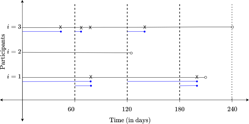
Figure 1: Visualization of recurrent events in both traditional format (black) and censored longitudinal format (blue). Start times of follow-up windows ($\mathcal{T}=\{0,60,120,180\text{ days}\}$, with $a=60$) are highlighted by vertical dashed lines. Traditional observed recurrent event data for individuals $i=1,2,3$ are $\big{\{}\{X^{*}_{1,1}=80,\delta_{1,1}=1\},\{X^{*}_{2,1}=125,\delta_{2,1}=0\},\{X^{*}_{3,1}=48,\delta_{1,1}=1\},\{X^{*}_{3,2}=62,\delta_{1,2}=1\},\{X^{*}_{3,3}=75,\delta_{1,3}=1\},\{X^{*}_{3,4}=147,\delta_{1,4}=1\},\{X^{*}_{3,5}=240,\delta_{1,5}=0\}\big{\}}$ . For these same individuals, the observed censored longitudinal data visualized here is $\big{\{}\{X_{1}(0)=80,\delta_{1}(0)=1\},\{X_{1}(60)=20,\delta_{1}(60)=1\},\{X_{1}(120)=83,\delta_{1}(120)=1\},\{X_{1}(180)=23,\delta_{1}(180)=1\},\big{\{}\{X_{2}(0)=125,\delta_{2}(0)=0\},\{X_{2}(60)=65,\delta_{2}(60)=0\},\{X_{2}(120)=5,\delta_{2}(120)=0\},\big{\{}\{X_{3}(0)=48,\delta_{3}(0)=1\},\{X_{3}(60)=2,\delta_{3}(60)=1\},\{X_{3}(120)=27,\delta_{3}(120)=1\},\{X_{3}(180)=60,\delta_{3}(180)=0\}\big{\}}$. All participants were administratively censored after 8 months (240 days). Participant 2 has no recorded events before $C_{2}$. Additionally, while $X^{*}_{33}$ is technically observed, it is not included in the censored longitudinal data set because it is the second observation in the window, and there is no $t$ such that $X_{i}(t)=X^{*}_{33}$. Besides potential correlation between separate event times seen in the same individual, this data structure induces correlation due to the same event contributing to the final censored longitudinal values in more than one follow-up window. For example, $X^{*}_{12}$ produces two measures in the longitudinal data structure, $X_{1}(120)=83$ and $X_{1}(180)=23$.

3 Random Forest for Uncensored Longitudinal Outcomes: A Review

Regression trees are a popular approach to incorporating multi-way interactions among predictors by finding groups of observations that are similar. A tree is grown in a few steps where at each step a new branch sorts the data leftover from the preceding step into bins based on one of the predictors. The sequential branching slices the space of predictors into rectangular partitions and approximates the true outcome-predictor relationship with the average outcome within each partition. Therefore, to grow a tree is to find bins that best discriminate among the outcomes. The specific predictor and the value split at each branching are chosen to minimize prediction error.

The number of possible trees is combinatorically large and precludes efficient global optimization (the number of binary trees with $K$ leaves is $(2K-3)!!$). Greedy algorithms have been developed to approximate the optimal global tree by myopically optimizing prediction error at the start of each branch. We will focus on binary trees in this paper for their popularity and effectiveness. The loss associated with the prediction error for a branch is often termed “impurity” which measures how similarly the observations behave on either side of the binary split. The branching procedure halts, for example, when the number of observations in a terminal node or the number of terminal nodes reaches respective thresholds. Advantages of a regression tree include invariance to monotonic transformation of predictors, flexible approximation to potentially severe nonlinearities, and the capacity to approximate $L-1$ way interactions for a tree with depth $L$.

To overcome potential overfitting, ensemble methods can be used to combine predictions from many trees into a single prediction. Random forest is such a ensemble regularizer based on Breiman’s bootstrap aggregation (Breiman, 2001), or “bagging,” which averages over multiple predictions obtained from trees grown from multiple bootstrap samples hence stabilizing the overall prediction. Random forest is a variation of bagging designed to further reduce the correlation among trees grown using different bootstrap samples by “dropout” which considers only a randomly drawn subset of predictors for splitting at each potential branch. Such a strategy ensures that early branches for some trees will not always split on predictors that offer the most gain in prediction accuracy. This reduces the correlation among predictions by multiple trees to further improve the variance reduction relative to the standard bagging along with reduced computational cost.

Among the many variants of random forest, we are particularly interested in random forests for longitudinal data, as recurrent event analysis uses data obtained from subjects over time. Adler et al. (2011) proposed an algorithm for tree-based ensemble methods that takes into consideration the dependence structure inherent in longitudinal data analysis. We provide a primer on this specific variation of random forest.

Let $(Y_{i}(t)$, $\bm{Z}_{i}(t))$ be a pair of a continuous outcome and a set of $p$-dimensional covariates, measured at time $t\in\mathcal{T}_{i}$ for $i=1,2,...,n$; here we use ${\mathcal{T}}_{i}$’s introduced in Section 2 with shared measurement timings to align more closely with our construction in Section 4, although the algorithm presented herein is applicable to scenarios with subject-specific measurement timings. In Section 4, we will substitute $Y_{i}(t)$ here with a longitudinal outcome ($\widehat{S}_{i}^{\tau}(t)$) that is constructed based on pseudo-observation technique to overcome censoring. Also note that the $\bm{Z}_{i}(t)$ may include time $t$. The following algorithm assumes $Y_{i}(t)=g\{\bm{Z}_{i}(t)\}+\epsilon_{i}(t)$ with $\mathbb{E}[\epsilon_{i}(t)]=0$ and is designed to estimate $g(\cdot)$ which describes a potentially complex relationship between the outcome and the predictors.

For $b=1,\ldots,B$, we repeat Step 1 and 2 below ($B=500$ is used in this manuscript):

• (Bootstrap): Generate a bootstrap sample $\{(Y_{i}(t),\bm{Z}_{i}(t)),(i,t)\in Bootstrap(b)\}$ from the original data set, where $Bootstrap(b)$ is the $b$-th bootstrap sample; Bootstrap(b) is obtained by first sampling $n$ subjects with replacement, followed by drawing a random check-in time point $t\in\{t_{0},t_{1},...,t_{m_{i}}\}$ for each bootstrapped subject $i$ (Adler et al., 2011). This data from follow-up times selected from individuals in $Bootstrap(b)$ is called bagged, and data not in the sample is called out-of-bag.

• (Grow a tree): Initialize the tree stump by grouping all observations together.

  • (Form split variables) At a potential branching, randomly select $m$ predictors from the $p$ predictors with $m\ll p$; in this paper we use the default choice of $m=\sqrt{p}$ which works well in our simulation and data analysis. Let the randomly selected predictors be $\{Z_{i,s_{1}}(t),\ldots,Z_{i,s_{m}}(t)\}$ at a particular potential branching for bagged observation $(i,t)$ where $(s_{1},\ldots,s_{m})$ are the indices for the subset of $m$ predictors. For ease of presentation, we denote it by $\bm{W}=(W_{1},\ldots,W_{m})$. For a continuous or categorical observed covariate $W_{k}$, construct a grid of all observed values of the covariate, $\tilde{W}_{k}=\{w_{kl},l=1,\ldots,L_{k}\}$. Consider all possible thresholds in $\tilde{W}_{k}$ and their corresponding indicators, $\{I(Z_{i,s_{k}}(t)<w_{kl}),(i,t)\in Bootstrap(b),w_{kl}\in\tilde{W_{k}}\}$ for the a subject $i$ at check-in time $t$ in the bootstrap sample $Boostrap(b)$. These derived indicator functions for continuous and categorical covariates, along with covariates in $\bm{W}$ that were already binary, are potential split variables.

  • (Choose branching): Choosing a covariate among $\bm{W}$ and the split value $w_{kl}$ will result in two daughter nodes, $\{N_{w_{kl},1},N_{w_{kl},0}\}$. Criteria for selecting the best variable and split vary by outcome type and metric of prediction accuracy. For continuous outcomes, the split with minimal sum of squared errors (SSE), is selected, though for other responses types, loss functions such as the Gini Index may be selected. For any particular node split under consideration using covariate $w$, that partitions individuals into two groups ($\{N_{w,0},N_{w,1}\}$) of sizes $n_{w,0}$ and $n_{w,1}$, we minimize the criterion $SSE(w)=\sum_{c=0,1}\sum_{q=1}^{n_{w,c}}(Y_{q}-\overline{Y_{c}})^{2}$, where $\overline{Y_{c}}=\frac{1}{n_{w,c}}\sum_{q=1}^{n_{w,c}}Y_{q,c}=0,1$.

  • (Stopping criteria and prediction from the grown tree) Repeat Step 2a and 2b until one of the following hyperparameters has been met: minimum node size ($\min\{n_{w,c},c=0,1\}$) is set to $40$ in this paper) is reached, or $SSE(w)$ does not decrease any further with more branches. This results in a single binary decision tree. For each terminal node (“leaf”) of the tree $C$, predict $Y_{i}(t)$ by the average of the outcome for observations in leaf $C$. Let the prediction be $\widehat{Y}_{b}(\bm{Z}_{i}(t);\widehat{\bm{\theta}}_{b})$, where $\widehat{\bm{\theta}}_{b}$ is the collection of terminal node predictions in the $b$-th tree.

• (Ensemble prediction by random forest): The final prediction for an individual $i^{\prime}$ with covariates $\bm{Z}_{i^{\prime}}(t)$ is given by the average of all the outputs from $B$ binary decision trees above: $\widehat{Y}_{i^{\prime}}(t)=\frac{1}{B}\sum_{b=1}^{B}\widehat{Y}_{b}(\bm{Z}_{i^{\prime}}(t);\widehat{\bm{\theta}}_{b})$.

Remark 1

The two-stage bootstrapping scheme has a few statistical and computational advantages compared to a scheme that uses all observations within a bootstrapped subject: 1) it samples one observation per subject which makes it likely that different trees are trained by different measures within a subject, although the same subject might be selected; this further reduced the similarity between the fitted trees (Hu and Szymczak, 2023); 2) it makes the algorithm applicable to subjects with different numbers of measures while ensuring that covariates measured on individuals with longer follow-up time do not overpower those who have shorter follow-up periods (Adler et al., 2011).

Permutation tests are applied to the out-of-bag sample to generate $p$-values assessing statistical significance for predictors used within the random forest algorithm while controlling for the remaining predictors. Each variable, $W$, is selected and the values of $W$ in the out-of-bag sample are permuted $d$ times, to obtain $\mathscr{W}_{s}$, $s=1,2,...d$. This breaks their association with $Y(t)$. The out-of-bag samples corresponding to both $\mathscr{W}_{s}$ and $\mathit{W}$ are then passed through the forest to obtain new predictions, $\mathcal{P}_{\mathscr{W},s}$ and $\mathcal{P}_{\mathit{W}}$ respectively. Exploiting the fact that $\dfrac{\frac{1}{d}\sum_{s=1}^{d}(\mathcal{P}_{W}-\mathcal{P}_{\mathscr{W},s})}{\sigma_{\mathscr{W},\mathit{W}}}$ has an asymptotically standard normal distribution, one can then obtain a Wald-type test of variable significance ($\sigma_{\mathscr{W},\mathit{W}}$ is estimated from the permutation distribution of prediction errors).

Random forests for survival data can be evaluated using Harrell’s C-statistic (also called “C-index”), a non-parametric measure of concordance (Harrell et al., 1982). Briefly, the C-statistic compares the predicted risk scores or fit values for any two observations with the actual time-to-event for those two observations. The proportion of observations that are correctly ordered is reported as the C-index. Any model which perfectly orders patients based on some risk score has a C-index of 1, while a model with no predictive power has C-index equal to 0.50.

In the next section we review pseudo-observation methodology that can convert the censored longitudinal data developed in Section 2 into a version that can be used with the above algorithm.

4 Construction of Pseudo-Observations

Pseudo-observations are a variation of jack-knife methodology applicable to censored time-to-event outcomes (Andersen et al., 2003). This technical device has been used successfully for a single time-to-event and recurrent events in manuscripts such as: Andrei and Murray (2007); Hengelbrock et al. (2016); Xia et al. (2020); Zhao et al. (2020). Essentially a pseudo-observation of a censored outcome, once created, can be used in regression contexts as if it was an uncensored outcome. In this section, we will first describe the mechanics of how to create a pseudo-observation for each potentially censored time-to-first event in a follow-up window of length $\tau$ starting at $t$. We will then briefly describe properties of pseudo-observations in the context of the random forest described in Section 3.

In this manuscript, our parameter of interest is survival probability, but we recognize that pseudo-observation is a technique that can be applied to other targets, including $\tau$-restricted mean survival time and hazard estimation. To construct pseudo-observations to be used with our random forest algorithm, we return to the censored longitudinal data structure described in Section 2. We calculate two estimates of the probability of recurrent-event-free in a follow-up window of length $\tau$ beginning at check-in time $t$: $\widehat{P}(X_{i}(t)\geq\tau)$ and $\widehat{P}^{(-i)}(X_{i}(t)\geq\tau)$ via the Kaplan-Meier estimator without conditioning on any covariate information for an individual $i=1,2,...,n(t)$ at risk at time $t$, where $\widehat{P}^{(-i)}(X_{i}(t)\geq\tau)$ is estimated excluding individual $i$. The pseudo-observation for individual $i$ at time $t$ is defined by:

$$\widehat{S}^{\tau}_{i}(t)=n(t)\widehat{P}(X_{i}(t)\geq\tau)-(n(t)-1)\widehat{P}^{(-i)}(X_{i}(t)\geq\tau).$$

To gain intuition behind the use of pseudo-observations, consider the simplest case where there is no censoring. Then, algebraically, $\widehat{P}(T_{i}(t)\geq\tau)=\frac{\sum_{j=1}^{n(t)}I(T_{j}(t)\geq\tau)}{n(t)}$ and $\widehat{P}^{(-i)}(T_{i}(t)\geq\tau)=\frac{\sum_{j\neq i,j=1}^{n(t)}I(T_{j}(t)\geq\tau)}{n(t)-1}$. Here $\widehat{S}_{i}^{\tau}(t)$ reduces to $I(T_{i}(t)\geq\tau)$, so that $E[\widehat{S}_{i}^{\tau}(t)\mid\bm{Z}_{i}(t)]=E[I(T_{i}(t)\geq\tau)|\bm{Z}_{i}(t)]=P(T_{i}(t)\geq\tau|\bm{Z}_{i}(t))$. This property is approximately held when we use Kaplan-Meier estimates for $\widehat{P}(T_{i}(t)\geq\tau)$ and $\widehat{P}^{(-i)}(T_{i}(t)\geq\tau)$ in the independent right-censored case. Andersen et al. (2003) argued that this property enables consistent estimation by directly regressing the pseudo-observations upon covariates. When pseudo-observations of probability of time-to-first-recurrent-events are applied to random forests in Section 3 for prediction, we call the algorithm “RFRE.PO” (short for “Random Forest for Recurrent Events based on Pseudo-Observations”).

5 Simulation Study

In this section, we demonstrate the ability of RFRE.PO to predict $P(T_{i}(t)\geq\tau\mid\bm{Z}_{i}(t))$ in a scenario where the true relationship between $\bm{Z}_{i}(t)$ and $I(T_{i}(t)\geq\tau)$ is many times more complicated than a modeler who tends to depend on main effect terms would anticipate. In this section we first describe Model A, the ad hoc nonlinear Xia, Murray and Tayob (XMT) model (Xia et al., 2020) that perfectly reflects the relationship between $\bm{Z}_{i}(t)$ and $T_{i}(t)$; and the XMT model that only uses main effect terms for the $\bm{Z}_{i}(t)$ in its regression model (Model B). We will then describe details of how data were simulated for our study.

An interesting question arises when considering the covariates used in modeling. We intended to incorporate subject-specific event-history in some form as a covariate and initially worked under the assumption that this covariate would be available even for the first follow-up window. In settings with correlated outcomes, one would expect this to be an important term in a model, and yet many studies do not have such a history variable available as a covariate in the first follow-up window. Hence for each modeling strategy (RFRE.PO, Model A, Model B), we consider availability of three derived historical variable types: (1) none, where there is no history covariate available (2) full, where the history covariate is available for each individual $i$ in each follow-up window starting at $t\in\mathcal{T}_{i}$ or (3) partial, where the history covariate is only recorded for windows beginning at $t>t_{0}$.

The true relationship between recurrent events ($T_{i,1}<T_{i,2}<\ldots$) and patient characteristics (continuous covariates $Z_{1}$, $Z_{2}$, $Z_{4}$, and categorical covariates $Z_{3}$, $Z_{5}$, $Z_{6}$, $Z_{7}$) is designed to be intentionally complex. We generate the recurrent events by simulating and transforming possibly dependent gap-times by Gaussian copula. The recurrent event gap-times marginally follow an exponential distribution with hazard:

$$\lambda_{i}=\exp\{Z_{i2}\sin(Z_{i1}/Z_{i6})-Z_{i3}I(Z_{i2}>2)+Z_{i3}I(Z_{i2}\leq 2)+Z_{i1}Z_{i6}+Z_{i2}^{2}Z_{i4}\}.$$

We simulate $Z_{1}\sim N(0,5)$, $Z_{2}\sim N(2,0.8)$, $Z_{3}+2\sim\text{Poisson}(4)$, $Z_{4}-0.1\sim\text{Beta}(7,1)$, $Z_{5}\in\{0,1,2\}$ with probability $\big{(}\frac{2}{3},\frac{1}{6},\frac{1}{6}\big{)}$, $Z_{6}\in\{-5,-2,2,3\}$ with probability $\big{(}\frac{1}{10},\frac{1}{3},\frac{11}{30},\frac{1}{5}\big{)},$ and $Z_{7}\in\{0,1,2,3\}$ with equal probability. Individuals with simulated hazards outside of the range of $\frac{8}{15}$ and $15$ years are removed from the sample and replaced. We induce correlation among exponentially distributed gap times for each subject $i$ by utilizing the Gaussian copula method as described by Xia et al. (2020), for $\rho=0,0.3,0.6$ or $0.9$. The resultant recurrent event times are converted to a censored longitudinal data format as described in Section 2. Censoring is independently generated from an exponential distribution so that 0%, $23\%$, $45\%$, or $63\%$ of observations are censored before the end of the study.

The censored longitudinal data structure assumes $\mathcal{T}=\{0,\frac{1}{12},\frac{1}{6},...2\text{ years}\}$, and $\tau=\frac{1}{6}$ year. The XMT model estimates $\text{logit}\{E(S^{\tau}_{i}(t))\}$ assuming the relationship $\text{logit}\{E(S^{\tau}_{i}(t))\}=\mathbf{\beta}^{\top}\bm{Z}^{*}_{i}(t)$. For Model A, the ad hoc nonlinear model, $\bm{Z}^{*}_{i}(t)=\{Z_{i2}\sin(Z_{i1}/Z_{i6}),$ $(-1)^{I(Z_{i2}>2)}Z_{i3},$ $Z_{i1}Z_{i6},$ $Z_{i2}^{2}Z_{i4}\}^{\top}$. Note that in Xia et al. (2020), the XMT model was for modeling the restricted mean rather than $\widehat{S}^{\tau}_{i}(t)$; however, their methods extend easily to our case so we keep the same name of “XMT”. Model B (the main effects XMT model) has covariate vector $\bm{Z}^{*}_{i}(t)=\{Z_{i1},$ $Z_{i2},$ $Z_{i3},$ $Z_{i4},$ $Z_{i5},$ $Z_{i6},$ $Z_{i7}\}^{\top}$. A derived historical covariate, not already included in Model A will be added to augmented $\bm{Z}_{i}(t)$ in the full and partial scenarios, $H_{f,i}(t)$ and $H_{p,i}(t)$ respectively. At a particular window start time $t_{k}$, $H_{f,i}(t_{k})=\frac{\sum_{t\in\mathcal{T^{+}}_{i},t<t_{k}}\min\{X_{i}(t),\frac{1}{12}\text{ years}\}}{\sum_{t\in\mathcal{T}^{+}_{i}}I(t<t_{k})}$, and $H_{p,i}(t_{k})=\frac{\sum_{t\in\mathcal{T}_{i},t_{0}<t<t_{k}}\min\{X_{i}(t),\frac{1}{12}\text{ years}\}+\widehat{H}_{p,i}(t_{0})}{\sum_{t\in\mathcal{T}^{+}_{i}}I(t<t_{k})}$, where $\mathcal{T}^{+}_{i}=\{t_{0}-\frac{1}{12}\text{ years}\}\cup\mathcal{T}_{i}$, $\widehat{H}_{p,i}(t_{0})=\min{(\tilde{X}_{i}(t_{0}),\frac{1}{12}\text{ years})}$. $\tilde{X}_{i}(t_{0})$ is multiply imputed from an approximate Exponential($7.5$) distribution, consistent with clinician knowledge of recurrent event rates in the population. Hence results from partial scenarios will be combined across 10 imputed data sets in the partial history setting.

For each of the models described above, as well as RFRE.PO, Table 1 lists the mean and empirical standard deviation of the index of concordance of the algorithms discussed and Figure 2 shows the distribution of the index of concordance of the algorithms discussed. Increasing levels of correlation between recurrent event times are listed from left to right. As one moves down the table and figure, censoring levels increase.

For all levels of censoring, correlation and historical covariate use, excluding the highest correlation level with historical covariate use, Model A (the ad hoc nonlinear XMT model) has the best C-index with varying degrees of superiority to Model B (the main effects XMT model) and RFRE.PO method. The RFRE.PO approach outperforms Model B in all settings, except high correlation with use of covariate history, in which Model B competes with both RFRE.PO and Model A. This suggests that in highly correlated settings, patient history is more important than baseline covariate information.

In the absence of correlation, use of $H_{p}(t)$ in Model B weakens predictive performance, whereas predictive performance is similar for the Model B with $H_{f}(t)$ versus without use of $H_{f}(t)$. The RFRE.PO procedure is able to make large gains in predictive ability from use of $H_{p}(t)$ and $H_{f}(t)$ in the same case with no correlation. Generally, use of $H_{f}(t)$ gives superior predictive performance to use of $H_{p}(t)$ in settings with correlation between recurrent event times. Our summary of the RFRE.PO results is that any use of covariate history in settings with and without correlated recurrent event outcomes is quite important and assists in recovering information from the data as censoring increases.

Table 1: Simulated C-statistics listed as Mean (ESD) for varying prediction algorithms, censoring percentages (none is 0%, light is 23%, moderate is 45%, and heavy is 63%), and gap-time correlations ($\rho=0$, $0.3$, $0.6$, $0.9$). 300 replicates were performed with $n=500$ for each replicate.

	${\rho=0}$	${\rho=0.3}$	${\rho=0.6}$	${\rho=0.9}$
		No Censoring
Model A	0.677 (0.006)	0.672 (0.007)	0.664 (0.008)	0.651 (0.010)
RFRE.PO	0.598 (0.014)	0.589 (0.015)	0.576 (0.016)	0.558 (0.016)
Model B	0.530 (0.007)	0.531 (0.009)	0.531 (0.010)	0.529 (0.011)
Model A with $H_{p}(t)$	0.675 (0.006)	0.674 (0.007)	0.684 (0.007)	0.710 (0.007)
RFRE.PO with $H_{p}(t)$	0.629 (0.007)	0.651 (0.007)	0.683 (0.008)	0.710 (0.008)
Model B with $H_{p}(t)$	0.489 (0.023)	0.582 (0.019)	0.666 (0.011)	0.724 (0.009)
Model A with $H_{f}(t)$	0.676 (0.006)	0.677 (0.006)	0.691 (0.011)	0.712 (0.010)
RFRE.PO with $H_{f}(t)$	0.634 (0.008)	0.658 (0.007)	0.686 (0.009)	0.710 (0.007)
Model B with $H_{f}(t)$	0.519 (0.035)	0.645 (0.035)	0.685 (0.017)	0.731 (0.010)
		Light Censoring
Model A	0.676 (0.006)	0.672 (0.008)	0.665 (0.009)	0.650 (0.011)
RFRE.PO	0.594 (0.014)	0.585 (0.014)	0.574 (0.016)	0.557 (0.016)
Model B	0.530 (0.009)	0.531 (0.009)	0.532 (0.010)	0.530 (0.011)
Model A with $H_{p}(t)$	0.676 (0.007)	0.673 (0.008)	0.681 (0.007)	0.704 (0.008)
RFRE.PO with $H_{p}(t)$	0.628 (0.008)	0.649 (0.008)	0.680 (0.006)	0.707 (0.007)
Model B with $H_{p}(t)$	0.491 (0.025)	0.574 (0.019)	0.659 (0.013)	0.717 (0.011)
Model A with $H_{f}(t)$	0.675 (0.006)	0.677 (0.007)	0.689 (0.010)	0.705 (0.010)
RFRE.PO with $H_{f}(t)$	0.631 (0.008)	0.655 (0.008)	0.684 (0.008)	0.707 (0.008)
Model B with $H_{f}(t)$	0.523 (0.037)	0.642 (0.017)	0.680 (0.019)	0.724 (0.011)
		Moderate Censoring
Model A	0.676 (0.007)	0.672 (0.007)	0.664 (0.009)	0.649 (0.012)
RFRE.PO	0.591 (0.014)	0.584 (0.015)	0.570 (0.015)	0.555 (0.017)
Model B	0.531 (0.009)	0.532 (0.010)	0.531 (0.010)	0.530 (0.012)
Model A with $H_{p}(t)$	0.675 (0.007)	0.672 (0.008)	0.679 (0.008)	0.701 (0.008)
RFRE.PO with $H_{p}(t)$	0.623 (0.009)	0.644 (0.008)	0.676 (0.007)	0.705 (0.007)
Model B with $H_{p}(t)$	0.492 (0.023)	0.565 (0.021)	0.649 (0.015)	0.712 (0.012)
Model A with $H_{f}(t)$	0.675 (0.007)	0.676 (0.007)	0.686 (0.011)	0.700 (0.011)
RFRE.PO with $H_{f}(t)$	0.629 (0.009)	0.653 (0.008)	0.680 (0.009)	0.704 (0.008)
Model B with $H_{f}(t)$	0.528 (0.034)	0.639 (0.016)	0.674 (0.021)	0.718 (0.012)
		Heavy Censoring
Model A	0.676 (0.007)	0.672 (0.009)	0.664 (0.010)	0.649 (0.011)
RFRE.PO	0.586 (0.017)	0.577 (0.016)	0.568 (0.018)	0.551 (0.017)
Model B	0.532 (0.009)	0.532 (0.009)	0.533 (0.012)	0.530 (0.012)
Model A with $H_{p}(t)$	0.674 (0.007)	0.672 (0.009)	0.676 (0.009)	0.695 (0.009)
RFRE.PO with $H_{p}(t)$	0.618 (0.010)	0.640 (0.009)	0.671 (0.008)	0.700 (0.007)
Model B with $H_{p}(t)$	0.492 (0.025)	0.554 (0.022)	0.640 (0.016)	0.703 (0.013)
Model A with $H_{f}(t)$	0.675 (0.007)	0.675 (0.008)	0.684 (0.011)	0.695 (0.012)
RFRE.PO with $H_{f}(t)$	0.625 (0.010)	0.650 (0.009)	0.676 (0.009)	0.700 (0.009)
Model B with $H_{f}(t)$	0.531 (0.032)	0.636 (0.016)	0.668 (0.024)	0.711 (0.014)

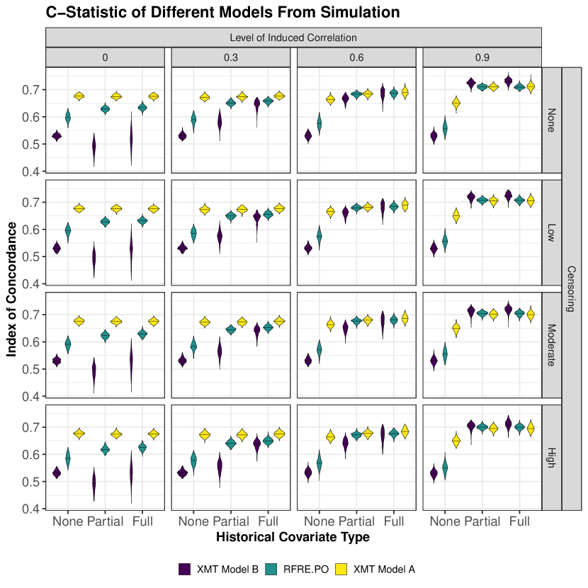
Figure 2: A violin plot of the distributions of the C-statistic of the models under consideration in simulation. Measures of center and spread can be found in Table 1. Within a box, historical covariate information increases from left to right. For partial history information, the distribution for the average C-statistic from $m=10$ imputed data sets is displayed.

6 Prediction of COPD Exacerbations

Chronic obstructive pulmonary disease (COPD) is most often attributed to a smoking history, although cases may also be caused by breathing polluted air such as biomass fuel or industrial chemicals (Safiri et al., 2022). COPD is characterized by periods of relative stability punctuated with episodic exacerbations of coughing, struggling for breath, and/or wheezing. Exacerbations may or may not result in hospitalization, in which case they are called severe. Such exacerbations increase overall disease progression, eventually leading to lung transplantation or death (Seemungal et al., 1998; Donaldson et al., 2002). Therefore, it is of clinical interest to dynamically predict the chances of being exacerbation-free over time.

We apply RFRE.PO to predict the probability of remaining exacerbation-free over a subsequent $\tau=180$ day follow-up period, using data from Azithromycin for the Prevention of COPD (Albert et al., 2011). Azithromycin for the Prevention of COPD was a multi-center clinical trial, aiming to estimate the treatment effect 250mg of oral azithromycin had on reducing exacerbations in COPD patients. Our example is applied to study participants ($n=1035$) who have complete baseline data, as well as longitudinal sleep study variables. Recurrent exacerbations were monitored over the following year. There are 962 covariates measured, including demographic variables, social well-being surveys, sleep quality metrics and clinical characteristics such as FVC, and medication use. There is strong correlation between variables as some are derived from each other, making RFRE.PO an attractive alternative to model-based predictions (see Supplemental Figure LABEL:fig:corrHeatMap). Censored longitudinal data is constructed with $\mathcal{T}=\{0,30,60,...,180\}$ and used for all analyses shown in this section.

Baseline information on the time since the most recent exacerbation was not available. Hence in this study we are in a scenario similar to the partial history scenario in Section 5. In this example, we create two partial history variables, $H_{p_{1}}(t)$ and $H_{p_{2}}(t)$. $H_{p_{1}}(t)$ was assumed to take a categorical form based on whether the participant had an exacerbation in the past zero to 30 days, 31-92 days, 93-182 days, 183 days to 365 days, or finally, if that time was more than 365 days or never. $H_{p_{2}}(t)$ is 100 times the estimated 30-day event rate using all follow-up prior to time $t$ (so as to provide point estimates on a reasonable scale). For the first $H_{p_{1}}(0)$ and $H_{p_{2}}(0)$, multiple imputation was based on event rates in the placebo group for all participants, and Rubin’s rule (Rubin, 1987) was used to combine inference across multiply imputed datasets as appropriate.

For comparison purposes, we present RFRE.PO results alongside results from two XMT models, where XMT models are fit via the geese command from the geepack library in R. The first XMT model (Model 1) uses the same predictors identified in Xia et al. (2020) for this cohort, where these predictors were based on clinical judgement for estimating treatment effect, adjusted for known confounders. The second XMT model (Model 2) is based on Wald forward selection applied to the first multiply imputed data set with $p<0.05$ required for entry; covariates that introduce model instability are discarded from consideration. Prediction algorithms for RFRE.PO and Model 2 were applied to a training cohort (70% of original cohort) and all algorithms were evaluated via the C-statistic in a validation cohort (remaining 30% of original cohort). For any particular multiply imputed validation dataset, standard errors of the C-statistic are calculated via the bootstrap with $b=100$ bootstrap samples. C-statistics for models involving multiply imputed history variables are combined across multiply imputed datasets using Rubin’s rule. Parameter estimates and standard errors for Model 2, which involves the imputed partial history covariates, are combined across multiply imputed validation datasets via Rubin’s Rule. Permutation tests associated with the RFRE.PO algorithm predictors are calculated within the training dataset, using out-of-bag samples as described in Section 3.

For Model 1, where estimation of treatment effect, and not necessarily prediction was the goal, predictors that were identified as important in Xia et al. (2020) were baseline forced expiratory volume in liters (FEV), age in decades (Age10), gender (0 for female, 1 for male), and smoking status at baseline (Smoker):

$$\text{logit}\{E({S}^{\tau}_{i}(t))\}= \beta_{0}+\beta_{1}I(\text{Treatment})_{i}+\beta_{2}(\text{Baseline FEV})_{i}+$$

$$\beta_{3}(\text{Age10})_{i}+\beta_{4}I(\text{Male})_{i}+\beta_{5}I(\text{Smoker})_{i},$$

where parameter estimates are displayed in Supplemental Table LABEL:table:summer-estimates.

Model 2, the Wald forward selection model, is:

$$\text{logit}\{E({S}^{\tau}_{i}(t))\}=\beta_{0}+\beta_{1}I(H_{p_{1}}=\text{Exacerbation in 0 -30 days prior to time }t)_{i}+$$

$$\quad\beta_{2}I(\text{Bronchiectasis diagnosis before time }t)_{i}+\beta_{3}I(\text{Male gender})_{i}+$$

$$\quad\beta_{4}I(\text{Azithromycin group})_{i}+\beta_{5}I(\text{Non-selective beta-blocker use at time }t)_{i}+$$

$$\quad\beta_{6}I(\text{Mixed beta-blocker use at time }t)_{i}+\beta_{7}(\text{FEV}_{1}\text{/FVC \% predicted at time }t)_{i}+$$

$$\quad\beta_{8}(\text{SGRQ symptoms at time }t)_{i}+\beta_{9}I(\text{Supplemental oxygen use at time }t)_{i}+$$

$$\quad\beta_{10}I(\text{Hospitalization one year before study start})_{i}+\beta_{11}H_{p_{2}}(t)_{i}+$$

$$\quad\beta_{12}I(\text{Inhaled corticosteroid and long-acting muscarinic antagonist use at time }t)_{i}+$$

$$\quad\beta_{13}I(\text{Inhaled corticosteroid and long-acting beta-agonist use at time }t)_{i},$$

with parameter estimates displayed in Supplemental Table LABEL:table:wald-estimates.

For the RFRE.PO algorithm, Supplemental Table LABEL:table:perm-tests displays the corresponding p-values of the permutation tests, combined across multiply imputed datasets via Rubin’s rule. Predictors in Supplemental Table LABEL:table:perm-tests had a statistically significant permutation test z-score for at least one of the multiply imputed training datasets. Additional predictors that did not achieve statistical significance via the permutation test, but were used in the RFRE.PO algorithm in some form, are not shown.

Figure 3 displays the Z-scores for predictors included in Models 1 and 2 (validation dataset) or Table LABEL:table:perm-tests (out-of-bag samples from training dataset). As seen in Section 5, history variables were among the most important variables in the RFRE.PO approaches as well as the XMT model selected through Wald Z-score forward selection. While there is overlap between predictors included in the various algorithms, in terms of the C-statistic evaluated in the validation cohort, the RFRE.PO algorithm outperformed both the algorithm based on clinical input (Model 1) and the Wald forward selection model (Model 2) (C-statistic $0.616$ compared to $0.565$ and $0.550$, respectively, see Table 2). A large number of variables that were included in the random forest algorithm had statistical significance at the level of $0.05$ via the permutation test in at least one of the multiply imputed datasets (see Figure 3 for the z-statistic and p-values in Supplemental Table LABEL:table:perm-tests for the predictors deemed important). Statistically significant variables from Model 1 are similarly listed as important RFRE.PO predictors. Variables identified via Wald forward selection in Model 2 are for the most part identified as important variables in the RFRE.PO algorithm. The version of the predictors may vary between these two approaches. For example, variables related to the long-acting muscarinic or bronchodilator, and/or steroid treatment are incorporated in different forms into these models. Similarly, different heart medications are featured in Model 2 (beta-blockers) versus the RFRE.PO algorithm (anti-coagulants). The RFRE.PO algorithm highlights a few variables that were not used in Model 2, including pain level at time $t$ and leukocytosis present at time $t$. The RFRE.PO algorithm has no problem including information from correlated predictors; for instance two included variables measure pain (pain level at time $t$, standardized pain level at time $t$) and two included variables measure general health (general health score at time $t$ standardized general health score at time $t$).

The C-statistic corresponding to Model 1, which benefits from prior clinical knowledge of the causal pathway, validated well. The RFRE.PO random forest algorithm includes predictors, with corresponding split decisions, that minimize squared error of the predictions relative to the observed data. This results in predictor information that is included without rigorous checks for statistical significance, so validation in an independent data set is quite important when using this type of algorithm. Because Model 2 requires statistical significance of all included predictors, its individual predictors already have some theoretical validity built into the selection mechanism. However, with variable power to detect statistical significance of useful predictors, the comparisons with methods that do not require statistical significance will leave Model 2-style strategies at a disadvantage.

The RFRE.PO algorithm is completely agnostic to statistical significance and scientific experience, so long as the squared error within nodes along cut-points decreases. And although it may occasionally include a predictor that is not useful in the validation set (Type I Error analog), it has a much better chance of including predictors that are useful but would not have met statistical significance (akin to a Type II error) in traditional statistical model building environments. If the scientific goal of analysis is prediction, the RFRE.PO approach seems remarkably simple, effective, and reproducible.

Table 2: Comparison of the C-statistics of models fit to the validation set of the Azithromycin in the Prevention of COPD cohort. Models 1 and 2 are fit using the XMT approach. Model 1 is the model selected using clinician input from Xia et al. (2020). Model 2 includes predictors through automated forward selection requiring $p<0.05$ for entry into the model. Missing values in Model 2 and RFRE.PO for time since most recent exacerbation are multiply imputed using the coding scheme described in Section 6. RFRE.PO processes our random forest approach using the same predictors considered in Model 2. C-statistic estimates and standard errors for all methods and models are averaged across results from multiply imputed data with Rubin’s rule applied to bootstrapped ($b=100$) C-statistic standard errors.

Model Name	C-Statistic
	Mean	Standard Error
RFRE.PO	$0.616$	$0.009$
Model 1	$0.565$	$0.009$
Model 2	$0.550$	$0.010$

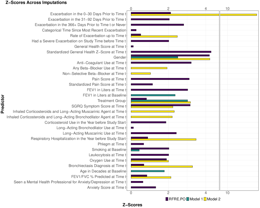
Figure 3: Wald Statistic Z-scores derived from the validation set for predictors that were included in Models 1 (XMT Xia, Murray, Tayob 2020 Model) and 2 (XMT Wald Forward Selection) after adjusting for multiple imputation using Rubin’s Rule, where appropriate, and permutation test Z-scores derived from out-of-bag samples as part of the RFRE.PO algorithm, adjusting for multiple imputation using Rubin’s Rule where appropriate. For the RFRE.PO method, 100 permutations were used in calculating the permutation Z-scores. Note that some Wald forward selection variables lost significance as additional terms were added.

7 Discussion

In this paper we presented a novel method for dynamically estimating probability of event-free survival during different follow-up windows. Using RFRE.PO, we showed the utility of our method in simulation, comparing its performance to traditional longitudinal model fits with an XMT model. In all instances, except for the most highly correlated, RFRE.PO outperformed the main effects XMT model that a traditional modeler might first attempt to fit. In instances of high correlation, RFRE.PO and the main effects model competed with the ad hoc nonlinear XMT model- that is, the perfect model that exactly reflected how the data were simulated.

An attractive feature of random forest applied to longitudinal follow-up windows is that a split based on the follow-up window times can occur and predictors that are more helpful in later follow up times can emerge naturally in importance. We explored recent history prior to the beginning of each follow-up window as a covariate in the algorithm, and found that it was one of the most useful predictors in settings with high correlation between recurrent events.

It is always important when introducing a new piece of methodology to clearly identify research questions that it can and cannot address. Random forest technology in general is aimed towards prediction, and for RFRE.PO, predicting the probability of remaining event-free during subsequent follow-up windows after patient check-ins. In this case, all available predictors that the treating clinician can access are valid and important to use. There is no goal, per sé, of establishing which predictors are statistically significant or have causal relationships with the outcomes. It is likely that some, if not most, of the predictors with high variable importance scores have these features, but metrics assessing statistical significance and causality are not necessarily valid for these algorithms.

In contrast, models such as the XMT model for recurrent event outcomes often have the goal of measuring the impact of a particular predictor or set of predictors on the outcome via an effect size, confidence interval and p-value. In the Azithromycin for Prevention of COPD cohort, the azithromycin effect was the key research question, requiring a measure of statistical significance as part of the drug approval process. Some predictors that would be very helpful in prediction are not allowed in these models assessing treatment effect. For instance, it is well-known that one should not include updates to patient characteristics after treatment has been initiated if these characteristics could have been improved by treatment; doing so would adjust away part of the treatment effect under study. Similarly, clinical trial analyses often require careful adjustment for confounders. If the goal is prediction and not assessment of treatment effect, these same confounders might not be included in the algorithm and in fact may not be helpful relative to other available predictors.

The ability of flexible algorithms like RFRE.PO to sift through large numbers of correlated predictors with complicated relationships to outcomes is an argument for their use over traditional reliance on models such as the XMT model. The growing popularity of machine learning tools is likely to dominate analyses of high-dimensional data, and the RFRE.PO algorithm contributes to this literature as one of the first machine learning methods to be able to make dynamic predictions from recurrent event data.

Data Availability Statement

Code for simulation and data analysis is available at https://github.com/AbigailLoe/RFRE.PO. The data that support the findings in this paper are available from the corresponding author upon reasonable request.

Supporting Information

Web Appendices and Figures referenced and R programs are available with this paper at the Biometrics website on Wiley Online Library.

References

- Adler et al. (2011) Adler, W., Potapov, S., and Lausen, B. (2011). Classification of repeated measurements data using tree-based ensemble methods. Computational Statistics 26, 355–369.
- Albert et al. (2011) Albert, R. K., Connett, J., Bailey, W., Casaburi, R., Cooper, A., Criner, G., Curtis, J., Dransfield, M., Han, M., Lazarus, S., Make, B., Marchetti, N., Martinez, F., Madinger, N., McEvoy, C., Niewoehner, D., Porsasz, J., Price, C., Reily, J., Scanlon, P., Sciurba, F., Scharf, S., Washko, G., Woodruff, P., and Anthonisen, N. (2011). Azithromycin for prevention of exacerbations of copd. New England Journal of Medicine 365, 689–698.
- Andersen and Gill (1982) Andersen, P. K. and Gill, R. D. (1982). Cox’s regression model for counting processes: A large sample study. The Annals of Statistics 10, 1100–1120.
- Andersen et al. (2003) Andersen, P. K., Klein, J. P., and Rosthøj, S. (2003). Generalised linear models for correlated pseudo-observations, with applications to multi-state models. Biometrika 90, 15–27.
- Andrei and Murray (2007) Andrei, A.-C. and Murray, S. (2007). Regression models for the mean of the quality-of-life-adjusted restricted survival time using pseudo-observations. Biometrics 63, 398–404.
- Ang et al. (2009) Ang, Y., Meyerson, L., Tang, Y., and Qian, N. (2009). Statistical methods for the analysis of relapse data in ms clinical trials. Journal of Neurological Sciences 285, 206–211.
- Breiman (2001) Breiman, L. (2001). Random forests. Machine Learning 45, 5–32.
- Breiman et al. (1984) Breiman, L., Freidman, J. H., Olshen, R. A., and Stone, C. J. (1984). CART: Classification and Regression Trees.
- Chan and Wang (2017a) Chan, K. C. G. and Wang, M.-C. (2017a). Semiparametric modeling and estimation of the terminal behavior of recurrent marker processes before failure events. Journal of the American Statistical Association 112, 351–362.
- Chan and Wang (2017b) Chan, K. C. G. and Wang, M.-C. (2017b). Semiparametric modeling and estimation of the terminal behavior of recurrent marker processes before failure events. U.S. National Library of Medicine .
- Choi et al. (2017) Choi, S., Huang, X., Ju, H., and Ning, J. (2017). Semiparametric accelerated intensity models for correlated recurrent and terminal events. Statistica Sinica 27, 625–643.
- Donaldson et al. (2002) Donaldson, G., Seemungal, T., Bhowmik, A., and Wedzicha, J. (2002). Relationship between exacerbation frequency and lung function in chronic obstructive pulmonary disease. Thorax 57, 847–852.
- Gerber et al. (2021a) Gerber, G., Faou, Y. L., Lopez, O., and Trupin, M. (2021a). The impact of churn on client value in health insurance, evaluation using a random forest under various censoring mechanisms. Journal of the American Statistical Association 116, 2053–2064.
- Gerber et al. (2021b) Gerber, G., Faou, Y. L., Lopez, O., and Trupin, M. (2021b). The impact of churn on client value in health insurance, evaluation using a random forest under various censoring mechanisms. Journal of the American Statistical Association 116, 2053–2064.
- Harrell et al. (1982) Harrell, Frank E., J., Califf, R. M., Pryor, D. B., Lee, K. L., and Rosati, R. A. (1982). Evaluating the Yield of Medical Tests. Journal of the American Medical Association 247, 2543–2546.
- Hengelbrock et al. (2016) Hengelbrock, J., Gillhaus, J., Kloss, S., and Leverkus, F. (2016). Safety data from randomized controlled trials: applying models for recurrent events. Pharmaceutical Statistics 15, 315–323.
- Hu and Szymczak (2023) Hu, J. and Szymczak, S. (2023). A review on longitudinal data analysis with random forest. Briefings in Bioinformatics 2, 1–11.
- Ishwaran et al. (2004) Ishwaran, H., Blackstone, E. H., Pothier, C. E., and Lauer, M. S. (2004). Relative risk forests for exercise heart rate recovery as a predictor of mortality. Journal of the American Statistical Association 99, 591–600.
- Kong et al. (2016) Kong, M., Xu, S., Levy, S., and Datta, S. (2016). Gee type inference for clustered sero-inflated negative binomial regression with application to dental caries. Computational Statistics and Data Analysis 85, 54–66.
- Liang et al. (2017) Liang, B., Tong, X., Zeng, D., and Wang, Y. (2017). Semiparametric regression analysis of repeated current status data. Statistica Sinica 27, 1079–1100.
- Lin et al. (2000) Lin, D. Y., Wei, L.-J., Yang, I., and Ying, Z. (2000). Semiparametric regression for the mean and rate functions of recurrent events. Journal of the Royal Statistical Society: Series B (Statistical Methodology) 62, 711–730.
- Mao and Lin (2016) Mao, L. and Lin, D. Y. (2016). Semiparametric regression for the weighted composite endpoint of recurrent and terminal events. U.S. National Library of Medicine .
- Miloslavsky et al. (2004) Miloslavsky, M., Keleş, S., van der Laan, M. J., and Butler, S. (2004). Recurrent events analysis in the presence of time-dependent covariates and dependent censoring. Journal of the Royal Statistical Society. Series B (Statistical Methodology) 66, 239–257.
- Rubin (1987) Rubin, D. B. (1987). Multiple imputation for nonresponse in surveys.
- Safari et al. (2023) Safari, A., Petkau, J., FitzGerald, M. J., and Sadatsafavi, M. (2023). A parametric model to jointly characterize rate, duration, and severity of exacerbations in episodic diseases. BMC Medical Informatics and Decision Making 23, 1–11.
- Safiri et al. (2022) Safiri, S., Carson-Chahhoud, K., Noori, M., Nejadghaderi, S. A., Sullman, M. J. M., Heris, J. A., Ansarin, K., Mansournia, M. A., Collins, G. S., Kolahi, A.-A., and Kaufman, J. S. (2022). Burden of chronic obstructive pulmonary disease and its attributable risk factors in 204 countries and territories, 1990-2019: results from the global burden of disease study 2019. BMJ 378, e069679.
- Seemungal et al. (1998) Seemungal, T., Donaldson, G., Paul, E., Jeffries, D., and Wedzicha, J. (1998). Effect of Exacerbation on quality of life in patients with chronic obstructive pulmonary disease. American Journal of Critical Care Medicine 157, 1418–22.
- Tayob and Murray (2015) Tayob, N. and Murray, S. (2015). Nonparametric tests of treatment effect based on combined endpoints for mortality and recurrent events. Biostatistics 16, 73–83.
- Wager and Athey (2018) Wager, S. and Athey, S. (2018). Estimation and inference of heterogeneous treatment effects using random forests. Journal of the American Statistical Association 113, 1228–1242.
- Xia and Murray (2019) Xia, M. and Murray, S. (2019). Commentary on Tayob and Murray (2014) with a useful update pertaining to study design. Biostatistics 20, 542––545.
- Xia et al. (2020) Xia, M., Murray, S., and Tayob, N. (2020). Regression analysis of recurrent-event-free time from multiple follow-up windows. Statistics in Medicine 39, 1–15.
- Xu et al. (2017) Xu, G., Chiou, S. H., Huang, C.-Y., Wang, M.-C., and Yan, J. (2017). Joint scale-change models for recurrent events and failure time. Journal of the American Statistical Association 112, 794–805.
- Yokota and Matsuyama (2019) Yokota, I. and Matsuyama, Y. (2019). Dynamic prediction of repeated events data based on leanmakring model: application to colorectal liver metastases data. BMC Medical Research Methodology 19, 1–11.
- Zhao et al. (2020) Zhao, L., Murray, S., Mariani, L. H., and Ju, W. (2020). Incorporating longitudinal biomarkers for dynamic risk prediction in the era of big data: A pseudo-observation approach. Statistics in Medicine 39, 3685–3699.