Deep Unlearning: Fast and Efficient Training-free Approach to Controlled Forgetting

Abstract

Machine unlearning has emerged as a prominent and challenging area of interest, driven in large part by the rising regulatory demands for industries to delete user data upon request and the heightened awareness of privacy. Existing approaches either retrain models from scratch or use several finetuning steps for every deletion request, often constrained by computational resource limitations and restricted access to the original training data. In this work, we introduce a novel class unlearning algorithm designed to strategically eliminate an entire class or a group of classes from the learned model. To that end, our algorithm first estimates the Retain Space and the Forget Space, representing the feature or activation spaces for samples from classes to be retained and unlearned, respectively. To obtain these spaces, we propose a novel singular value decomposition-based technique that requires layer wise collection of network activations from a few forward passes through the network. We then compute the shared information between these spaces and remove it from the forget space to isolate class-discriminatory feature space for unlearning. Finally, we project the model weights in the orthogonal direction of the class-discriminatory space to obtain the unlearned model. We demonstrate our algorithm’s efficacy on ImageNet using a Vision Transformer with only $\sim 1.5\%$ drop in retain accuracy compared to the original model while maintaining under $1\%$ accuracy on the unlearned class samples. Further, our algorithm consistently performs well when subject to Membership Inference Attacks showing $7.8\%$ improvement on average across a variety of image classification datasets and network architectures, as compared to other baselines while being $\sim 6\times$ more computationally efficient. Additionally, we investigate the impact of unlearning on network decision boundaries and conduct saliency-based analysis to illustrate that the post-unlearning model struggles to identify class-discriminatory features from the forgotten classes.

1 Introduction

Machine learning has automated numerous applications in various domains, including image processing, language processing, and many others, often surpassing human performance. Nevertheless, the inherent strength of these algorithms, which lies in their extensive reliance on training data, paradoxically presents potential limitations. The literature has shed light on how these models behave as highly efficient data compressors (Tishby & Zaslavsky, 2015; Schelter, 2020), often exhibiting tendencies toward the memorization of full or partial training samples (Arpit, 2017; Bai et al., 2021). Such characteristics of these algorithms raise significant concerns about the privacy and safety of the general population. This is particularly concerning given that the vast training data, typically collected through various means like web scraping, crowdsourcing, user data collection through apps and services, and more, is not immune to personal and sensitive information. The growing awareness of these privacy concerns and the increasing need for safe deployment of these models have ignited discussions within the community and, ultimately, led to some regulations on data privacy, such as Voigt & Von dem Bussche (2017); Goldman (2020). These regulations allow the use of the data with the mandate to delete personal information pertaining to a user if they choose to opt-out from sharing their data. The mere deletion of data from archives is not sufficient due to the memorization behavior of these models. This necessitates machine unlearning algorithms that can remove the influence of requested data or unlearn those samples from the model. A naive approach, involving the retraining of models from scratch, guarantees the absence of information from sensitive samples but is often impractical, especially when dealing with compute intensive State-of-The-Art (SoTA) models like ViT(Dosovitskiy et al., 2020). Further, efficient unlearning poses considerable challenges, as the model parameters do not exhibit a straightforward connection to the training data (Shwartz-Ziv & Tishby, 2017). Moreover, these unlearning algorithms may only have access to a fraction of the original training data, further complicating the unlearning process.

Our work focuses on challenging scenarios of class unlearning and multi-class unlearning (task unlearning) (Golatkar et al., 2020a; 2021). For a class unlearning setup, the primary goal of the unlearning algorithm is to eliminate information associated with a target class from a pretrained model. This target class is referred to as the forget class, while the other classes are called the retain classes. The unlearning algorithm should produce parameters that are functionally indistinguishable to those of a model trained without the target class. The key challenges in such unlearning is three folds (i) pinpointing class-specific information within the model parameters, (ii) updating the weights in a way that effectively removes target class information without compromising the model’s usability on other classes and (iii) demonstrating scalability on large scale dataset with well trained models. The current SoTA for class unlearning (Tarun et al., 2023) shows acceptable accuracy on the retained classes compared to the original model, achieving minimal unlearning times. However, the authors present their results on undertrained models having $\sim 10\%$ lower accuracy for the original model on the entire dataset. The memorization behavior of the model is generally exhibited during the later training stages where the model overfits the training data (Feldman & Zhang, 2020) and it might not be fair to evaluate unlearning when the model is not trained to convergence. Additionally, the results of this work are presented only on small datasets like CIFAR10 and CIFAR100 (Krizhevsky et al., 2009). The practical use of such algorithms may be limited by their performance when applied to well-trained models on large-scale datasets. In this work, we ask the question “Can we unlearn class (or multiple classes) from a well trained model given access to few samples from the training data on a large dataset?”. Having a few samples is particularly interesting if the unlearning algorithms have to efficiently scale to large datasets having many classes to ensure fast and resource efficient unlearning algorithm.

We draw insights from work by Saha et al. (2021) in the domain of continual learning, where the authors use the Singular Value Decomposition (SVD) technique to estimate the gradient space essential for the previous task and restrict future updates in this space to maintain good performance on previous learning tasks. This work demonstrates a few samples ( about 125 samples per task ) are sufficient to obtain a good representation of the gradient space. Our work proposes to strategically eliminate the class discriminatory information by updating the model weights to maximally suppress the activations of the samples belonging to unlearn class. We first estimate the Retain Space and the Forget Space, representing the feature or activation spaces for samples from classes to be retained and unlearned, respectively. We propose a novel singular value decomposition-based technique to obtain these spaces, which requires layer wise collection of network activations from a few samples through the network. We then compute the shared information between these spaces and remove it from the forget space to isolate class-discriminatory feature space for unlearning. Finally, we project the model weights in the orthogonal direction of the class-discriminatory space to obtain the unlearned model. We demonstrate our algorithm on a simple 4 way classification problem with input containing 2 features as shown in Figure LABEL:fig:toy_problem. The decision boundary learnt by the trained model is shown in Figure LABEL:fig:original_decision_boundary while the model unlearning the red class exhibits the decision boundary depicted in Figure LABEL:fig:unlearnt_decision_boundary. The decision boundary for a retrained model is shown if Figure LABEL:fig:retrained This illustration shows that the proposed algorithm redistributes the input space of the class to be unlearnt to the closest classes. The experimental details of this demonstration are provided in Appendix A.1. Our algorithm demonstrates SOTA performance in class unlearning setup with access to very few samples from the training dataset ( less than $4\%$ for all our experiments). As our algorithm relies on very few samples from the train dataset it efficiently scales to large datasets like ImageNet (Deng et al., 2009), where we demonstrate the results using 1500 samples ($0.00117\%$ of the training dataset).

In summary, the contributions of this work are listed as follows,

• We propose a novel Singular Value decomposition based class unlearning algorithm which uses very few samples from the training data and does not rely on gradient based optimization steps. To the best of our knowledge, our work is the first to demonstrate class unlearning results on ImageNet for SoTA transformer based models.

• We evaluate our algorithm on various datasets and with a variety of models and show our algorithm consistently outperforms the State of the Art methods. Additionally, we provide evidence that our model’s behavior aligns with that of a model trained without the forget class samples through membership inference attacks, saliency-based feature analyses and confusion matrix analyses.

• We demonstrate the applicability of our algorithm to two practical scenarios in multi-class unlearning: (i) One-shot Multi-Class unlearning ( or task unlearning) through a single step of multi-class unlearning and (ii) Sequential Multi-Class unlearning through multiple steps of single class unlearning, demonstrating the capability of processing multiple unlearning requests over time.

2 Related Works

Unlearning: Many unlearning algorithms have been introduced in the literature, addressing various unlearning scenarios, including item unlearning (Bourtoule et al., 2021), feature unlearning (Warnecke et al., 2021), class unlearning (Tarun et al., 2023), and task unlearning (Parisi et al., 2019). Some of these solutions make simplifying assumptions on the learning algorithm. For instance, Ginart et al. (2019) demonstrate unlearning within the context of k-mean clustering, Brophy & Lowd (2021) present their algorithm for random forests, Mahadevan & Mathioudakis (2021) and Izzo et al. (2021) propose an algorithm in the context of linear/logistic regression. Further, there have been efforts in literature, to scale these algorithms for convolution layers Golatkar et al. (2020a; b). Note, however, the algorithms have been only demonstrated on small scale problems. In contrast, other works, such as Bourtoule et al. (2021), suggest altering the training process to enable efficient unlearning. This approach requires saving multiple snapshots of the model from different stages of training and involves retraining the model for a subset of the training data, effectively trading off compute and memory for good accuracy on retain samples. Unlike these works our proposed algorithm does not make any assumptions on the training process or the algorithm used for training the original model.

Class Unlearning: The current State-of-the-Art (SoTA) for class unlearning is claimed by Tarun et al. (2023). In their work, the authors propose a three stage unlearning process, where the first stage learns a noise pattern that maximizes the loss for each of the classes to be unlearnt. The Second stage (also called the impair stage) unlearns the class by mapping the noise to the forget class. Finally, if the impair stage is seen to reduce the accuracy on the retained classes, the authors propose to finetune the impaired model on the subset of training data in the repair stage (the third stage). This work presents the results on small datasets with undertrained models and utilizes up to $20\%$ of the training data for the unlearning process. Further, the work by Chundawat et al. (2023) proposes two algorithms which assumes no access to the training samples. Additionally, authors of Baumhauer et al. (2022) propose a linear filtration operator to shift the classification of samples from unlearn class to other classes. These works lose considerable accuracy on the retain class samples and have been demonstrated on small scale datasets like MNIST and CIFAR10. Our work demonstrates results on SoTA Vision transformer models for the ImageNet dataset, showing the effective scaling of our algorithm on large dataset with the model trained to convergence.

Other Related Algorithms : SVD is a well known technique used to constrain the learning in the direction of previously learnt tasks in the continual learning setup Saha et al. (2021); Chen et al. (2022); Saha & Roy (2023). These methods are sample efficient in estimating the gradient space relevant to a task. Recent work by Li et al. (2023) proposes subspace based federated unlearning using SVD. The authors perform gradient ascent in the orthogonal space of input gradient spaces formed by other clients to eliminate the target client’s contribution in a federated learning setup. Such ascent based unlearning is generally sensitive to hyperparameters and is susceptible to catastrophic forgetting on retain samples. As our proposed approach does not rely on such gradient based training steps it is less sensitive to the hyperparameters. Moreover, the techniques could be used on top of our method to further enhance the unlearning performance.

3 Preliminaries

Class Unlearning: Let the training dataset be denoted by $\mathcal{D}_{train}=\{(x_{i},y_{i})\}_{i=1}^{N_{train}}$ consisting of $N_{train}$ training samples where $x_{i}$ represents the network input and $y_{i}$ is the corresponding label. The test dataset be $\mathcal{D}_{test}=\{(x_{i},y_{i})\}_{i=1}^{N_{test}}$ containing $N_{test}$ samples. Consider a function $y=f(x_{i},\theta)$ with the parameters $\theta$ that approximates the mapping of the inputs $x_{i}$ to their respective labels $y_{i}$. In the case of a well-trained deep learning model with parameters $\theta$, there would be numerous samples $(x_{i},y_{i})\in\mathcal{D}_{test}$ for which the relationship $y_{i}=f(x_{i},\theta)$ holds. For a class unlearning task aimed at removing the target class $t$, the training dataset can be split into two partitions, namely the retain dataset $\mathcal{D}_{train\_r}=\{(x_{i},y_{i})\}_{i=1;y_{i}\neq t}^{N}$ and the forget dataset $\mathcal{D}_{train\_f}=\{(x_{i},y_{i})\}_{i=1;y_{i}=t}^{N}$. Similarly the test dataset can be split into these partitions as $\mathcal{D}_{test\_r}=\{(x_{i},y_{i})\}_{i=1;y_{i}\neq t}^{N}$ and $\mathcal{D}_{test\_f}=\{(x_{i},y_{i})\}_{i=1;y_{i}=t}^{N}$. The objective of the class unlearning algorithm is to derive unlearnt parameters $\theta^{*}_{f}$ based on $\theta$, a subset of the retain partition $\mathcal{D}_{train\_sub\_r}\subset\mathcal{D}_{train\_r}$, and a subset of the forget partition $\mathcal{D}_{train\_sub\_f}\subset\mathcal{D}_{train\_f}$. The parameters $\theta^{*}_{f}$ must be functionally indistinguishable from a network with parameters $\theta^{*}$, which is retrained from scratch on the samples of $\mathcal{D}_{\text{train\_r}}$ in the output space. In other words, these parameters must satisfy $f(x_{i},\theta^{*})\simeq f(x_{i},\theta^{*}_{f})$ for $(x_{i},y_{i})\in\mathcal{D}_{\text{test}}$ or $\mathcal{D}_{\text{train}}$.

SVD: A rectangular matrix $A\in\mathbb{R}^{d\times n}$ can be decomposed using SVD as $A=U\Sigma V^{T}$ where $U\in\mathbb{R}^{d\times d}$ and $V\in\mathbb{R}^{n\times n}$ are orthogonal matrices and $\Sigma\in\mathbb{R}^{d\times n}$ is a diagonal matrix containing singular values Deisenroth et al. (2020). The columns of matrix $U$ are the $d$ dimensional orthogonal vectors sorted by the amount of variance they explain for $n$ samples (or the columns) in the matrix $A$. These vectors are also called the basis vectors explaining the column space of A. For the $i^{th}$ vector in $U$, $u_{i}$, the amount of the variance explained is proportional to the square of the $i^{th}$ singular value $\sigma_{i}^{2}$. Hence the percentage variance explained by a basis vector $u_{i}$ is given by $\sigma_{i}^{2}/(\sum_{j=1}^{d}(\sigma_{j}^{2}))$.

4 Unlearning Algorithm

The pseudocode of our approach is presented in Algorithm 1. Consider $l^{th}$ layer of a network given by $x_{o}^{l}=x_{i}^{l}(\theta^{l})^{T}$, where $\theta^{l}$ signifies the parameters, $x_{i}^{l}$ stands for input activations and $x_{o}^{l}$ denotes output activation. Our algorithm aims to suppress the class-discriminatory activations associated with forget class. When provided with a class-discriminatory projection matrix $P_{dis}^{l}$, suppressing this class-discriminatory activation from the input activations gives us $x_{i}^{l}-x_{i}^{l}P_{dis}^{l}$. Post multiplying the parameters with $(I-P_{dis})^{T}$, is mathematically the same as removing class-discriminatory information from $x_{i}^{l}$ as shown in Equation 1. This enables us to modify the model parameters to destroy the class-discriminatory activations given the matrix $P_{dis}^{l}$ and is accomplished by the update_parameter() function in line 13 of Algorithm 1. The rest of this section focuses on optimally computing this class-discriminatory projection matrix $P_{dis}^{l}$.

(1)

Input: $\theta$ is the parameters of the original model; $X_{r}$ and $X_{f}$ is small set of inputs $x_{i}$ sampled independently from $\mathcal{D}_{train\_r}$ and $\mathcal{D}_{train\_f}$ respectively; $\mathcal{D}_{train\_sub\_r}\subset\mathcal{D}_{train\_r}$; $\mathcal{D}_{train\_sub\_f}\subset\mathcal{D}_{train\_f}$; and alpha_r_list and alpha_f_list are is list of hyperparameters $\alpha_{r}$ and $\alpha_{f}$ respectively.
1. procedure Unlearn( $\theta$, $X_{r}$, $X_{f}$, $\mathcal{D}_{train\_sub\_r}$, $\mathcal{D}_{train\_sub\_f}$, alpha_r_list, alpha_f_list )
2.     best_score = get_score($\theta$, $\mathcal{D}_{train\_sub\_r}$, $\mathcal{D}_{train\_sub\_f}$);      $\theta^{*}_{f}=\theta$
3.     $R_{r}$ = get_representation(model, $X_{r}$) //Collect representations of linear
4.     $R_{f}$ = get_representation(model, $X_{f}$) and convolution layers
5.     for each linear and convolution layer $l$ do
6.        $U_{r}^{l}$, $\Sigma_{r}^{l}$ = SVD($R_{r}^{l}$);      $U_{f}^{l}$, $\Sigma_{f}^{l}$ = SVD($R_{f}^{l}$) //Space Estimation for each layer
7.     for each $\alpha_{r}\in$ alpha_r_list do
8.        for each $\alpha_{f}\in$ alpha_f_list do
9.           for each linear and convolution layer $l$ do
10.            $\Lambda_{r}^{l}$ = scale_importance($\Sigma_{r}^{l}$, $\alpha_{r}$);      $\Lambda_{f}^{l}$ = scale_importance($\Sigma_{f}^{l}$, $\alpha_{f}$) //Eqn. 2
11.            $P_{r}^{l}$ = $U_{r}^{l}\Lambda_{r}^{l}$transpose( $U_{r}^{l}$);    $P_{f}^{l}$ = $U_{f}^{l}\Lambda_{f}^{l}$transpose($U_{f}^{l}$)
12.            $P_{dis}^{l}=P_{f}^{l}(I-P_{r}^{l})$ //class discriminatory projection matrix
13.            $\theta_{f}^{l}=$update_parameter($I-P_{dis}^{l}$, $\theta^{l}$ ) //parameter projection for $l^{th}$ layer
14.          score = get_score($\theta_{f}$, $\mathcal{D}_{train\_sub\_r}$, $\mathcal{D}_{train\_sub\_f}$)
15.          if score $>$ best_score do
16.             best_score = score;      $\theta^{*}_{f}=\theta_{f}$
17. return $\theta^{*}_{f}$

Algorithm 1 Pseudocode of Training Free Algorithm for Controlled forgetting

4.1 Class Discriminatory Space

In order to compute the class-discriminatory projection matrix, $P_{dis}^{l}$, we need to estimate the activation space for retain class samples and the forget class samples. These spaces, also referred as the Retain Space ($U_{r}^{l}$) and the Forget Space ($U_{f}^{l}$), are computed using SVD on the accumulated representations for the corresponding samples as elaborated in Section 4.1.1. Subsequently, we scale the basis vectors within their respective spaces using importance scores proportional to the variance explained by each vector. This yields the scaled retain projection matrix $P_{r}^{l}$ and the scaled forget projection matrix $P_{f}^{l}$. These scaled projection matrices are used to compute Class-discriminatory Projection matrix, $P_{dis}^{l}$, as explained in Section 4.1.2.

4.1.1 Space Estimation via SVD on Representations

In this Subsection, we provide the details on Space Estimation given by lines 3-6 of Algorithm 1. We give an in-depth explanation for obtaining the Retain Space, $U_{r}$. We use a small subset of samples from the classes to be retained, denoted as $X_{r}=\{x_{i}\}_{i=1}^{K_{r}}$, where $K_{r}$ represents the number of retain samples. Forget Space ($U_{f}$) is estimated similarly on the samples from the class to be unlearnt, denoted by $X_{f}=\{x_{i}\}_{i=1}^{K_{f}}$ where $K_{f}$ represents the number of samples.

Representation Matrix: To obtain the basis vectors for the Retain Space through SVD, we need to collect the representative information (activations) for each layer in the network and organize them into a representation matrix denoted as $R_{r}^{l}$. We accumulate these representation matrices, $R_{r}^{l}$, for both linear and convolutional layers in a list $R_{r}=[R_{r}^{l}]_{l=1}^{L}$, where $L$ is the number of layers. In the case of linear layer, this matrix is given by $R_{r}^{l}=[(x_{i}^{l})_{i=1}^{K_{r}}]$, which stacks the input activations $x_{i}^{l}$ to obtain a matrix of size $K_{r}\times d^{l}$, where $d^{l}$ is the input dimension of $l^{th}$ linear layer.

A convolutional layer has to be represented as a matrix multiplication to apply the proposed weight update rule. This is done using the unfold operation (Liu et al., 2018) on input activation maps. For a convolutional layer with $C_{i}$ input channels and $k$ as kernel size each sliding window has the size of $C_{i}\times k\times k$. If the output activation, $x_{o}^{l}$, has the resolution of $h_{o}\times w_{o}$, where $h_{o}$ and $w_{o}$ is the height and width of the output activations, then there are $h_{o}w_{o}$ patches of size $C_{i}\times k\times k$ in the input activation $x_{i}^{l}$. The convolution kernel operates on each of these patches in a sliding window fashion to get the values at the corresponding locations in the output map. The unfold operation flattens each of these $h_{o}w_{o}$ patches to get a matrix of size $h_{o}w_{o}\times C_{i}kk$. Now, if we reshape the weight as $C_{i}kk\times C_{o}$ where $C_{o}$ is the output channels, we see that the convolution operation becomes a matrix multiplication between the unfolded matrix and the reshaped weights achieving the intended objective. Hence, the representation matrix for the convolutional layer is given by $R^{l}_{r}=[($unfold($x_{i}^{l}$)${}^{T})_{i=1}^{K_{r}}]$. The representation matrix is obtained by get_representation() function in line 3 of the Alogithm 1.

Space Estimation: We perform SVD on the representation matrices for each layer as shown in line 6 of the Algorithm 1. SVD() function returns the basis vectors $U_{r}^{l}$ that span the activation of the retain samples in $X_{r}$ and the singular values $\Sigma_{r}^{l}$ for each layer $l$. Retain Space $U_{r}=[U_{r}^{l}]_{l=1}^{L}$ is the list of these basis vectors for all the layers.

4.1.2 Projection Space

The basis vectors in the Spaces obtained are orthonormal and do not capture any information about the importance of the basis vector. The information of the significance of the basis vector is given by the corresponding singular value. Hence, we propose to scale the basis vector in proportion to the amount of variance they explain in the input space as presented below.

Importance Scaling: To capture the importance the $i^{th}$ basis vector in the matrix $U$ (or the $i^{th}$ column of $U$), we formulate an diagonal importance matrix $\Lambda$ having the $i^{th}$ diagonal component $\lambda_{i}$ given by Equation 2. Here $\sigma_{i}$ represents the the $i^{th}$ singular value in the matrix $\Sigma$. The parameter $\alpha\in(0,\infty)$ called the scaling coefficient is a hyperparameter that controls the scaling of the basis vectors. When $\alpha$ is set to 1 the basis vectors are scaled by the amount of variance they explain. As $\alpha$ increases the importance score for each basis vector increases and reaches 1 as $\alpha\to\infty$. Similarly decrease in $\alpha$ decreases the importance of the basis vector and goes to 0 as $\alpha\to 0$. This operation is represented by scaled_importance() function in line 10 of the Algorithm 1. It is important to note that without the proposed scaling approach the matrices $P_{r}$ and $P_{f}$ become identity in line 11 of Algorithm 1, as $U$ is an orthonormal matrix. This inturn makes $P_{dis}$ a zero matrix, which means the weight update in line 13 of Algorithm 1 projects weight on identity matrix mathematically restricting unlearning. Hence it is important to use scaling in Line 10 of Algorithm 1

Scaled Projection Matrix ($P$): Say we have Spaces $U_{r}^{l}$ and $U_{f}^{l}$ for a layer with singular values $\Sigma_{r}^{l}$ and $\Sigma_{f}^{l}$ and the scaling coefficients are set to a value of $\alpha_{r}$ and $\alpha_{f}$. We can compute the importance scaling matrices $\Lambda_{r}$ and $\Lambda_{f}$ as per Equation 2. The scaled retain projection matrix, which projects the input activations to the retain space is given by $P_{r}^{l}=U_{r}^{l}\Lambda_{r}^{l}(U_{r}^{l})^{T}$ and the scaled forget projection matrix given by $P_{f}^{l}=U_{f}^{l}\Lambda_{f}^{l}(U_{f}^{l})^{T}$, see line 11 in Algorithm 1.

Class-Discriminatory Projection Matrix ($P_{dis}$): To obtain the unlearn class discriminatory projection matrix, we remove the shared space given by $P_{f}^{l}P_{r}^{l}$ from the forget projection matrix to obtain $P_{dis}^{l}=P_{f}^{l}-P_{f}^{l}P_{r}^{l}$. Alternatively, this can also be written as $P_{dis}^{l}=P_{f}^{l}(I-P_{r}^{l})$. Intuitively, this projects the forget space onto the space that does not contain any information about the retain space, effectively removing the shared information from the forget projection matrix to obtain the discriminatory projection space. Our algorithm introduces two hyperparameters namely $\alpha_{r}$ and $\alpha_{f}$ the scaling coefficients for the Retain Space and the Forget Space respectively. The next Subsection 4.2 presents a discussion on these hyperparameters.

4.2 Hyperparameter search

Our algorithm searches for the optimal hyperparameter values for $\alpha_{r}$ and $\alpha_{f}$ within the predefined lists provided as alpha_r_list and alpha_f_list, respectively. We observe this search is necessary for our algorithm. One intuitive explanation for this is that the unlearning class may exhibit varying degrees of confusion with the retain classes, making it easier to unlearn some classes compared to others, hence requiring different scaling for the retain and forget spaces. We introduce a simple scoring function given below to rank the unlearnt models with different pair of $\alpha_{r}$ and $\alpha_{f}$.

Score: The proposed scoring function given by Equation 3 returns penalized retain accuracy, where $acc_{r}$ and $acc_{f}$ are the accuracy on the $\mathcal{D}_{train\_sub\_r}$ and $\mathcal{D}_{train\_sub\_f}$ respectively. This function returns a low score for a unlearnt model having a high value of $acc_{f}$ or an unlearnt model having low $acc_{r}$. The value of the returned score is high only when $acc_{r}$ is high and $acc_{f}$ is low, which is the desired behavior of the unlearnt model.

Grid Search: Our algorithm begins with the best unlearn model parameters $\theta^{*}_{f}$ as the original model parameters $\theta$. As seen in line 7 and 8 of the Algorithm 1 we do a grid search over all the possible values of $\alpha_{r}$ and $\alpha_{f}$ provided in alpha_r_list and alpha_f_list to obtain the best unlearnt parameters $\theta^{*}_{f}$. Note, we observe that increasing the value of $\alpha_{f}$ decreases the retain accuracy $acc_{r}$ and hence we terminate the inner loop (line 8) to speed up the grid search and have not presented this in the Algorithm 1 for simplicity. Our approach only perform inference and does not rely on computationally intensive gradient based optimization steps (which also require tuning the learning rates) and gets the unlearnt model in a single step for each grid search (over $\alpha_{r}$ and $\alpha_{f}$) leading to a fast and efficient approach.

4.3 Discussion

The speed and efficiency of our approach can be attributed to the design choices. Firstly our method runs inference for very few samples to get the representations $R$. Further, the small sizes of these representation matrices ensure that SVD is fast and computationally cheap. Additionally, the SVD operation for each layer is independent and can be parallelized to further improve speeds. Our approach only performs inference and does not rely on computationally intensive gradient based optimization steps (which also require tuning the learning rates) and gets the unlearnt model in a single step for each grid search (over $\alpha_{r}$ and $\alpha_{f}$) leading to a fast and efficient approach. Additionally, our method has fewer parameters as compared to the gradient based baselines which are sensitive to the choices of optimizer, learning rate, batch size, learning rate scheduler, weight decay, etc. Further, our algorithm can be readily extended to Transformer architectures by applying our algorithm to all the linear layers in the architecture. Note, that we do not change the normalization layers for any architecture as the fraction of total parameters for these layers is insignificant. Further, our algorithm assumes a significant difference in the distribution of forget and retain samples for SVD to find distinguishable spaces. This is true in class unlearning setup, where retain and forget samples come from different non-overlapping classes. However, in the case of unlearning a random subset of training data, this assumption would not hold and our method has limited performance in such a scenario, requiring additional modification for effective unlearning.

5 Experiments

Dataset and Models : We conduct the class unlearning experiments on CIFAR10, CIFAR100 (Krizhevsky et al., 2009) and ImageNet (Deng et al., 2009) datasets. We use the modified versions of ResNet18 (He et al., 2016) and VGG11 (Simonyan & Zisserman, 2014) with batch normalization for the CIFAR10 and CIFAR100 datasets. These models are trained for 350 epochs using Stochastic Gradient Descent (SGD) with the learning rate of 0.01. We use Nesterov (Sutskever et al., 2013) accelerated momentum with a value of 0.9 and the weight decay is set to 5e-4. For the ImageNet dataset, we use the pretrained VGG11 and base version of Vision Transformer with a patch size of 14 (Dosovitskiy et al., 2020) available in the torchvision library.

Comparisons: We benchmark our method against 5 unlearning approaches. Two of these approaches, Retraining (Chundawat et al., 2023) and NegGrad (Tarun et al., 2023) are commonly used in literature. Retraining involves training the model from scratch using the retain partition of the training set, $D_{train\_r}$, and serves as our gold-standard model. In the NegGrad approach, we finetune the model for a few step using gradient ascent on the forget partition of the train set $D_{train\_f}$ with a gradient clipping threshold set at 0.25. This approach ensures good forgetting, however is seen to reduce the model accuracy on the retain partition. We also compare our approach to a stronger version of NegGrad called NegGrad+ proposed by Kurmanji et al. (2023). This algorithm does gradient ascent on the forget samples and gradient descent on the retain samples for 500 steps. A detailed explanation of NegGrad and NegGrad+ with psuedocodes is presented in Appendix A.2 and  LABEL:apx:neggrad_plus respectively. Finally, we compare our work with two SoTA algorithms (Tarun et al., 2023; Kurmanji et al., 2023) to demonstrate the effectiveness of our approach. Discussion on hyperparameters is presented in Appendix LABEL:apx:hyp.

Evaluation: Our experiments evaluate the accuracy on the unlearnt models with the accuracy on retain samples $ACC_{r}$ and the accuracy on the forget samples $ACC_{f}$. In addition, we implement Membership Inference Attack ($MIA$) to distinguish between samples in $\mathcal{D}_{train\_r}$ and $\mathcal{D}_{test\_r}$. We use the confidence scores for the target class and training a Support Vector Machine (SVM) (Hearst et al., 1998) classifier. We report the average model predictions on $\mathcal{D}_{train\_f}$ as the MIA scores in our evaluations. A high value of $MIA$ score for a given sample indicates that it does not belong to the training data. An unlearnt model is expected to match the $MIA$ score of the Retrained model. See Appendix LABEL:apx:mia for details on MIA experiment.

6 Results

Table 1: Results for Single class Forgetting on CIFAR10 and CIFAR100 dataset. (We bold font the row having highest value for $ACC_{r}(100-ACC_{f})MIA$)

	Method	VGG11_BN			ResNet18
		$ACC_{r}(\uparrow)$	$ACC_{f}(\downarrow)$	$MIA(\uparrow)$	$ACC_{r}(\uparrow)$	$ACC_{f}(\downarrow)$	$MIA(\uparrow)$
CIFAR10	Original	$91.58\pm 0.52$	$91.58\pm 4.72$	$0.11\pm 0.08$	$94.89\pm 0.31$	$94.89\pm 2.75$	$0.03\pm 0.03$
	Retraining	$92.58\pm 0.83$	$0$	$100\pm 0$	$94.81\pm 0.52$	$0$	$100\pm 0$
	NegGrad	$81.46\pm 5.67$	$0.02\pm 0.04$	$0$	$69.89\pm 10.23$	$0$	$0$
	NegGrad+	$89.79\pm 1.49$	$0.13\pm 0.16$	$99.93\pm 0.15$	$87.38\pm 1.36$	$0.2\pm 0.33$	$0$
	Tarun et al. (2023)	$89.21\pm 0.84$	$0$	$0$	$92.20\pm 0.72$	$10.89\pm 8.79$	$61.5\pm 25.86$
	Kurmanji et al. (2023)	$46.18\pm 35.376$	$0$	$0$	$80.28\pm 7.31$	$6.4\pm 19.074$	$0$
	Ours	$\textbf{91.77}\pm\textbf{0.69}$	0	$\textbf{98.28}\pm\textbf{5.43}$	$\textbf{94.19}\pm\textbf{0.50}$	$\textbf{0.03}\pm\textbf{0.09}$	$\textbf{95.5}\pm\textbf{14.23}$
CIFAR100	Original	$69.22\pm 0.29$	$67\pm 15.23$	$0.2\pm 0.25$	$76.64\pm 0.13$	$74.3\pm 13.27$	$0.08\pm 0.1$
	Retraining	$68.97\pm 0.40$	$0$	$100\pm 0$	$76.81\pm 0.50$	$0$	$100\pm 0$
	NegGrad	$51.21\pm 6.37$	$0$	$0$	$60.32\pm 7.03$	$0$	$29.98\pm 48.27$
	NegGrad+	$58.66\pm 3.91$	$0$	$0$	$71.37\pm 2.78$	$0$	$100\pm 0$
	Tarun et al. (2023)	$53.94\pm 1.22$	$0$	$0$	$63.387\pm 0.50$	$3.1\pm 5.65$	$0$
	Kurmanji et al. (2023)	$67.073\pm 0.41$	$10.5\pm 18.32$	$84.3\pm 26.76$	$72.54\pm 0.43$	$10.2\pm 16.90$	$89.28\pm 17.18$
	Ours	$\textbf{65.94}\pm\textbf{1.21}$	$\textbf{0.3}\pm\textbf{0.48}$	$\textbf{99.92}\pm\textbf{0.10}$	$\textbf{73.60}\pm\textbf{1.41}$	$\textbf{0.3}\pm\textbf{0.48}$	$\textbf{100}\pm\textbf{0}$

Table 2: Results for Single class forgetting on ImageNet-1k dataset.

Method	Total	VGG11_BN			ViT_B_16
	samples	$ACC_{r}(\uparrow)$	$ACC_{f}(\downarrow)$	$MIA(\uparrow)$	$ACC_{r}(\uparrow)$	$ACC_{f}(\downarrow)$	$MIA(\uparrow)$
Original	-	$68.61\pm 0.02$	$72.6\pm 25.92$	$22.72\pm 22.59$	$80.01\pm 0.037$	$80.6\pm 19.87$	$13.36\pm 12.94$
NegGrad+	32000	$66.37\pm 1.27$	$8.8\pm 11.48$	$96.58\pm 4.40$	$73.76\pm 1.46$	$0$	$99.98\pm 0.05$
Tarun et al. (2023)	9990	$43.5618\pm 0.59$	$0$	$98.96\pm 3.26$	$56.00\pm 3.47$	$38.8\pm 34.074$	$66.67\pm 50$
Kurmanji et al. (2023)	10000	$\textbf{67.29}\pm\textbf{0.34}$	0	$\textbf{99.92}\pm\textbf{0.15}$	$79.23\pm 0.19$	$56\pm 21.56$	$45.47\pm 20.62$
Ours	1499	$66.41\pm 0.60$	$0.6\pm 1.35$	$99.33\pm 0.90$	$\textbf{78.47}\pm\textbf{0.84}$	$\textbf{0.2}\pm\textbf{0.63}$	$\textbf{99.98}\pm\textbf{0.0}5$

Class Forgetting: We present the results for single class forgetting in Table 2 for the CIFAR10 and CIFAR100 dataset. The table presents results that include both the mean and standard deviation across 10 different target unlearning classes. CIFAR10 dataset is accessed for unlearning on each class and CIFAR100 is evaluated for every 10th starting from the first class. The Retraining approach matches the accuracy of the original model on retain samples and has $0\%$ accuracy on the forget samples, which is the expected upper bound. The $MIA$ accuracy for this model is $100\%$ which signifies that MIA model is certain that $\mathcal{D}_{train\_f}$ does not belong to the training data. The NegGrad method shows good forgetting with low $ACC_{f}$, however, performs poorly on $ACC_{r}$ and $MIA$ metrics. The NegGrad algorithm’s performance on retain samples is expected to be poor because it lacks information about the retain samples required to protect the relevant features. Further, this explains why NegGrad+ which performs gradient descent on the retain samples along with NegGrad can maintain impressive performance on retain accuracy with competitive forget accuracy. In some of our experiments, we observe that the NegGrad+ approach outperforms the SoTA benchmarks (Tarun et al., 2023) and (Kurmanji et al., 2023) which suggests the NegGrad+ approach is a strong baseline for class unlearning. Our proposed training free algorithm achieves a better tradeoff between the evaluation metrics when compared against all the baselines. Further, we observe the MIA numbers for our method close to the retrained model and better than all the baselines for most of our experiments. We demonstrate our algorithm easily scales to ImageNet without compromising its effectiveness, as seen in Table 2. Due to the training complexity of the experiments, we were not able to obtain retrained models for ImageNet. We observe that the results on CIFAR10 and CIFAR100 datasets consistently show $ACC_{f}$ to be 0 and the $MIA$ performance to be $100\%$. We, therefore, interpret the model with high $ACC_{r}$, $MIA$, and low $ACC_{f}$ as a better unlearnt model for these experiments. We conduct unlearning experiments on the ImageNet dataset for every 100th class starting from the first class, resulting in a total of 10 experiments. Our algorithm shows less than $1.5\%$ drop in $ACC_{r}$ as compared to the original model while maintaining less than $1\%$ forget accuracy for a well trained SoTA Transformed based model. The MIA scores for our model are nearly $100\%$ indicating that model the MIA model fails to recognize $\mathcal{D}_{train\_f}$ as part of training data. We observe that (Kurmanji et al., 2023) outperforms our method for a VGG11 model trained on ImageNet, however, requires access to $6\times$ more samples and requires more compute than our approach. We present 2 other variants of the proposed algorithm in Appendix LABEL:apx:projection_location.

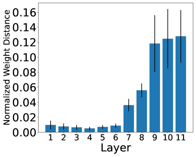
Figure 5: Layer-wise weight change for VGG11 on cifar10 dataset.

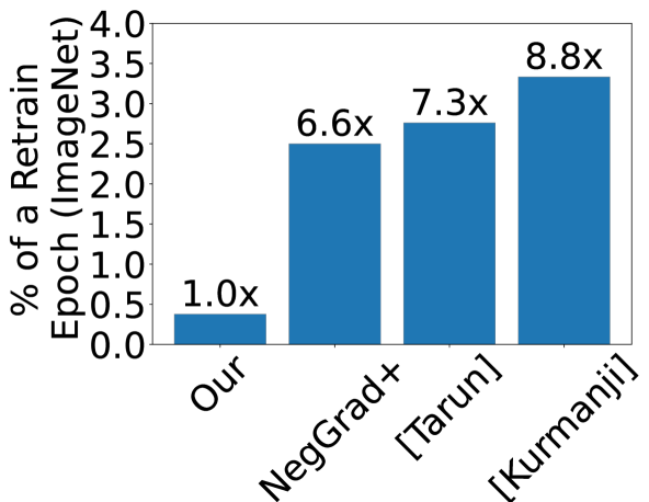
Figure 6: Compute comparison for single linear layer of ViT.

Confusion Matrix analysis: We plot the confusion matrix showing the distribution of true labels and predicted labels for the original VGG11 model and VGG11 model unlearning cat class with our algorithm for CIFAR10 in Figure LABEL:fig:cm. Interestingly, we observe that a significant portion of the cat samples are redistributed across the animal categories. The majority of these samples are assigned to the dog class, which exhibited the highest level of confusion with the cat class in the original model. This aligns with the illustration shown in Figure LABEL:fig:toy_problem where the forget space gets redistributed to the classes in the proximity of the forget class. We present the confusion matrix of the retrained VGG11 model without the cat class in Figure LABEL:fig:cm_retrain in Appendix LABEL:apx:cm_retrain. This matrix also shows a high number of cat samples being assigned to the dog class.

Saliency-based analysis : We test this VGG11 model unlearning the cat class with GradCAM-based feature analysis as presented in Figure LABEL:fig:gradcam, and we see that our model is unable to detect class discriminatory information. This behavior is similar to the retrained VGG11 model shown in Figure LABEL:fig:retrained_gradcam.

Layer-wise analysis: We plot the change layer-wise weight difference between the parameters of the unlearnt and the original model for VGG11 on the cifar10 dataset in Figure 5. We observe that the weight change is larger for the later layers. This is expected as the later layers are expected to learn complex class discriminatory information while the initial layers do learn edges and simple textures (Olah et al., 2017). We present the retain and forget accuracy when our algorithm is applied to the top layers in Appendix LABEL:apx:layer.

Compute analysis: We analytically calculate the computational cost for different unlearning algorithms for a Vision Transformer (ViT) model trained on ImageNet, as illustrated in Figure 6, see Appendix LABEL:apx:compute for details. This figure shows the percentage of compute cost as compared to a single epoch of retraining baseline on y axis. It’s important to note that we exclusively consider the computation of the linear layer ignoring the compute costs for self attention and normalization layers. This inherently works in favor of the gradient based approaches as our algorithm has significantly low overhead for these layers as we only do forward pass on a few samples while representation collection. Our approach demonstrates more than $6\times$ compute reduction than any other baseline.

Multi Class Forgetting: The objective of Multiclass removal is to remove more than one class from the trained model. In multi task learning a deep learning model is trained to do multiple tasks where each of the tasks is a group of classes. The scenario of One-Shot Multi-Class where the unlearning algorithm is expected to remove multiple classes in a single unlearning step has a practical use case in such task unlearning. Our algorithm estimates the Retain Space $U_{r}$ and the Forget Space $U_{f}$ based on the samples from $X_{r}$ and $X_{f}$. It is straightforward to scale our approach to such a scenario by simply changing the retain sample $X_{r}$ and $X_{f}$ to represent the samples from class to be retained and forgotten respectively. We demonstrate multi class unlearning on removing 5 classes belonging to a superclass on CIFAR100 dataset in Figure LABEL:fig:multi. We observe our method is able to retain good accuracy on Retain samples and has above $95\%$ MIA accuracy while maintaining a low accuracy on forget set under this scenario. When compared with Tarun et al. (2023) under this unlearning setting (see Table LABEL:tab:superclass in Appendix LABEL:apx:multiclass) we see our method has significantly better performance. We also present results of multiclass unlearning on CIFAR10 in Appendix LABEL:apx:multiclass. Additionally, we present a sequential version of multi class unlearning in Appendix LABEL:apx:seq_multiclass.

7 Conclusion

In this work, we introduce a novel class and multi-class unlearning algorithm based on Singular Value Decomposition (SVD), which eliminates the need for gradient-based unlearning steps. We demonstrate the efficacy of our approach over a variety of image classification datasets and network architectures. Our algorithm consistently performs better than SoTA on several evaluation metrics while being much more computationally efficient. Furthermore, to the best of our knowledge, our proposed class unlearning algorithm is the first to be demonstrated on large-scale datasets like ImageNet with a SoTA transformer based model. Our analysis, conducted through saliency-based explanations, does not reveal the class-discriminatory features, and the confusion matrix analysis shows the redistribution of the unlearned samples based on their confusion with respective classes.

Appendix A Appendix

A.1 Demonstration with Toy Example

In Figure LABEL:fig:toy_problem we demonstrate our unlearning algorithm on a 4 way classification problem, where the original model is trained to detect samples from 4 different 2-dimensional Gaussian’s centered around (1,1), (-1,1), (-1, -1) and (1, -1) respectively with a standard of (0.5,0.5). The training dataset has 10000 samples per class and the test dataset has 1000 samples per class. The test data is shown with dark points in the decision boundaries in Figure LABEL:fig:toy_problem. We use a simple 5-layer linear model with ReLU activation functions. All the intermediate layers have 5 neurons and each layer excluding the final layer is followed by BatchNorm. We train this network with stochastic gradient descent for 10 epochs with a learning rate of 0.1 and Nestrove momentum of 0.9. The decision boundary learnt by the original model trained on complete data is shown in Figure LABEL:fig:original_decision_boundary and the accuracy of this model on test data is $95.60\%$. In Figure LABEL:fig:unlearnt_decision_boundary we plot the decision boundary for the model obtained by unlearning the class with mean (1,1) with our algorithm. This decision boundary is observed to be close to the decision boundary of the model retrained without the data points from class with mean (1,1) as shown in Figure LABEL:fig:retrained. The accuracy of the unlearnt model is $97.43\%$ and retrained model is $97.33\%$. This illustration shows that the proposed algorithm redistributes the input space of the class to be unlearnt to the closest classes.

A.2 NegGrad Algorithm

Pseudocode for NegGrad is presented in Algorithm 2. The algorithm initialized the unlearn parameters $\theta^{*}_{f}$ to the original parameters $\theta$ and does $500$ steps of gradient ascent on the forget subset of the training data. After every 100 steps, we evaluate the model accuracy on $\mathcal{D}_{train\_sub\_f}$ and exit ascent when $acc_{f}$ becomes lower than 0.1. This restricts the gradient ascent from catastrophically forgetting the samples in the retain partition.

Input: $\theta$ is the parameters of the original model, $\mathcal{L}$ is the loss function, $\mathcal{D}_{train\_sub\_f}$ is the subset of the forget partition of the train dataset; and $\eta$ is the learning rate

1. procedure Unlearn( $\theta$, $\mathcal{L}$, $\mathcal{D}_{train\_sub\_f}$, $\eta$ )
2.     $\theta^{*}_{f}=\theta$
3.     for step = 1,…., 500 do
4.         input, target = get_batch($\mathcal{D}_{train\_sub\_f}$)
5.         $g$ = get_gradients($\theta^{*}_{f}$, $\mathcal{L}$, input, target)
6.         $g$ = gradient_clip($g$,$0.25$)
7.         $\theta^{*}_{f}$ = $\theta^{*}_{f}$ + $\eta$$g$
8.         if step multiple of 100 do
9.             $acc_{f}$ = get_accuracy($\theta$, $\mathcal{D}_{train\_sub\_f}$)
10.           breakif $acc_{f}<0.1$
11. return $\theta^{*}_{f}$

Algorithm 2 NegGrad Algorithm

References

- Arpit (2017) Devansh et. al. Arpit. A closer look at memorization in deep networks. In International conference on machine learning, pp. 233–242. PMLR, 2017.
- Bai et al. (2021) Ching-Yuan Bai, Hsuan-Tien Lin, Colin Raffel, and Wendy Chi-wen Kan. On training sample memorization: Lessons from benchmarking generative modeling with a large-scale competition. In Proceedings of the 27th ACM SIGKDD Conference on Knowledge Discovery & Data Mining, pp. 2534–2542, 2021.
- Baumhauer et al. (2022) Thomas Baumhauer, Pascal Schöttle, and Matthias Zeppelzauer. Machine unlearning: Linear filtration for logit-based classifiers. Machine Learning, 111(9):3203–3226, 2022.
- Bourtoule et al. (2021) Lucas Bourtoule, Varun Chandrasekaran, Christopher A Choquette-Choo, Hengrui Jia, Adelin Travers, Baiwu Zhang, David Lie, and Nicolas Papernot. Machine unlearning. In 2021 IEEE Symposium on Security and Privacy (SP), pp. 141–159. IEEE, 2021.
- Brophy & Lowd (2021) Jonathan Brophy and Daniel Lowd. Machine unlearning for random forests. In International Conference on Machine Learning, pp. 1092–1104. PMLR, 2021.
- Chen et al. (2022) Cheng Chen, Ji Zhang, Jingkuan Song, and Lianli Gao. Class gradient projection for continual learning. In Proceedings of the 30th ACM International Conference on Multimedia, pp. 5575–5583, 2022.
- Chundawat et al. (2023) Vikram S Chundawat, Ayush K Tarun, Murari Mandal, and Mohan Kankanhalli. Zero-shot machine unlearning. IEEE Transactions on Information Forensics and Security, 2023.
- Cline & Dhillon (2006) Alan Kaylor Cline and Inderjit S Dhillon. Computation of the singular value decomposition. In Handbook of linear algebra, pp. 45–1. Chapman and Hall/CRC, 2006.
- Deisenroth et al. (2020) Marc Peter Deisenroth, A. Aldo Faisal, and Cheng Soon Ong. Mathematics for Machine Learning. Cambridge University Press, 2020.
- Deng et al. (2009) Jia Deng, Wei Dong, Richard Socher, Li-Jia Li, Kai Li, and Li Fei-Fei. Imagenet: A large-scale hierarchical image database. In 2009 IEEE Conference on Computer Vision and Pattern Recognition, pp. 248–255, 2009. doi: 10.1109/CVPR.2009.5206848.
- Dosovitskiy et al. (2020) Alexey Dosovitskiy, Lucas Beyer, Alexander Kolesnikov, Dirk Weissenborn, Xiaohua Zhai, Thomas Unterthiner, Mostafa Dehghani, Matthias Minderer, Georg Heigold, Sylvain Gelly, et al. An image is worth 16x16 words: Transformers for image recognition at scale. arXiv preprint arXiv:2010.11929, 2020.
- Feldman & Zhang (2020) Vitaly Feldman and Chiyuan Zhang. What neural networks memorize and why: Discovering the long tail via influence estimation. Advances in Neural Information Processing Systems, 33:2881–2891, 2020.
- Ginart et al. (2019) Antonio Ginart, Melody Guan, Gregory Valiant, and James Y Zou. Making ai forget you: Data deletion in machine learning. Advances in neural information processing systems, 32, 2019.
- Golatkar et al. (2020a) Aditya Golatkar, Alessandro Achille, and Stefano Soatto. Eternal sunshine of the spotless net: Selective forgetting in deep networks. In Proceedings of the IEEE/CVF Conference on Computer Vision and Pattern Recognition, pp. 9304–9312, 2020a.
- Golatkar et al. (2020b) Aditya Golatkar, Alessandro Achille, and Stefano Soatto. Forgetting outside the box: Scrubbing deep networks of information accessible from input-output observations. In Computer Vision–ECCV 2020: 16th European Conference, Glasgow, UK, August 23–28, 2020, Proceedings, Part XXIX 16, pp. 383–398. Springer, 2020b.
- Golatkar et al. (2021) Aditya Golatkar, Alessandro Achille, Avinash Ravichandran, Marzia Polito, and Stefano Soatto. Mixed-privacy forgetting in deep networks. In Proceedings of the IEEE/CVF conference on computer vision and pattern recognition, pp. 792–801, 2021.
- Goldman (2020) Eric Goldman. An introduction to the california consumer privacy act (ccpa). Santa Clara Univ. Legal Studies Research Paper, 2020.
- He et al. (2016) Kaiming He, Xiangyu Zhang, Shaoqing Ren, and Jian Sun. Deep residual learning for image recognition. In Proceedings of the IEEE conference on computer vision and pattern recognition, pp. 770–778, 2016.
- Hearst et al. (1998) Marti A. Hearst, Susan T Dumais, Edgar Osuna, John Platt, and Bernhard Scholkopf. Support vector machines. IEEE Intelligent Systems and their applications, 13(4):18–28, 1998.
- Izzo et al. (2021) Zachary Izzo, Mary Anne Smart, Kamalika Chaudhuri, and James Zou. Approximate data deletion from machine learning models. In International Conference on Artificial Intelligence and Statistics, pp. 2008–2016. PMLR, 2021.
- Krizhevsky et al. (2009) Alex Krizhevsky, Geoffrey Hinton, et al. Learning multiple layers of features from tiny images. CIFAR, 2009.
- Kurmanji et al. (2023) Meghdad Kurmanji, Peter Triantafillou, and Eleni Triantafillou. Towards unbounded machine unlearning. arXiv preprint arXiv:2302.09880, 2023.
- Li et al. (2023) Guanghao Li, Li Shen, Yan Sun, Yue Hu, Han Hu, and Dacheng Tao. Subspace based federated unlearning. arXiv preprint arXiv:2302.12448, 2023.
- Liu et al. (2018) Zhenhua Liu, Jizheng Xu, Xiulian Peng, and Ruiqin Xiong. Frequency-domain dynamic pruning for convolutional neural networks. Advances in neural information processing systems, 31, 2018.
- Mahadevan & Mathioudakis (2021) Ananth Mahadevan and Michael Mathioudakis. Certifiable machine unlearning for linear models. arXiv preprint arXiv:2106.15093, 2021.
- Olah et al. (2017) Chris Olah, Alexander Mordvintsev, and Ludwig Schubert. Feature visualization. Distill, 2(11):e7, 2017.
- Parisi et al. (2019) German I Parisi, Ronald Kemker, Jose L Part, Christopher Kanan, and Stefan Wermter. Continual lifelong learning with neural networks: A review. Neural networks, 113:54–71, 2019.
- Saha & Roy (2023) Gobinda Saha and Kaushik Roy. Continual learning with scaled gradient projection. Proceedings of the AAAI Conference on Artificial Intelligence, 37(8):9677–9685, Jun. 2023. doi: 10.1609/aaai.v37i8.26157. URL https://ojs.aaai.org/index.php/AAAI/article/view/26157.
- Saha et al. (2021) Gobinda Saha, Isha Garg, and Kaushik Roy. Gradient projection memory for continual learning. In International Conference on Learning Representations, 2021. URL https://openreview.net/forum?id=3AOj0RCNC2.
- Schelter (2020) Sebastian Schelter. Amnesia-a selection of machine learning models that can forget user data very fast. suicide, 8364(44035):46992, 2020.
- Shwartz-Ziv & Tishby (2017) Ravid Shwartz-Ziv and Naftali Tishby. Opening the black box of deep neural networks via information. arXiv preprint arXiv:1703.00810, 2017.
- Simonyan & Zisserman (2014) Karen Simonyan and Andrew Zisserman. Very deep convolutional networks for large-scale image recognition. arXiv preprint arXiv:1409.1556, 2014.
- Sutskever et al. (2013) Ilya Sutskever, James Martens, George Dahl, and Geoffrey Hinton. On the importance of initialization and momentum in deep learning. In International conference on machine learning, pp. 1139–1147. PMLR, 2013.
- Tarun et al. (2023) Ayush K Tarun, Vikram S Chundawat, Murari Mandal, and Mohan Kankanhalli. Fast yet effective machine unlearning. IEEE Transactions on Neural Networks and Learning Systems, 2023.
- Tishby & Zaslavsky (2015) Naftali Tishby and Noga Zaslavsky. Deep learning and the information bottleneck principle. In 2015 ieee information theory workshop (itw), pp. 1–5. IEEE, 2015.
- Voigt & Von dem Bussche (2017) Paul Voigt and Axel Von dem Bussche. The eu general data protection regulation (gdpr). A Practical Guide, 1st Ed., Cham: Springer International Publishing, 10(3152676):10–5555, 2017.
- Warnecke et al. (2021) Alexander Warnecke, Lukas Pirch, Christian Wressnegger, and Konrad Rieck. Machine unlearning of features and labels. arXiv preprint arXiv:2108.11577, 2021.