Scalable Meta-Learning with Gaussian Processes

Abstract

Meta-learning is a powerful approach that exploits historical data to quickly solve new tasks from the same distribution. In the low-data regime, methods based on the closed-form posterior of Gaussian processes (GP) together with Bayesian optimization have achieved high performance. However, these methods are either computationally expensive or introduce assumptions that hinder a principled propagation of uncertainty between task models. This may disrupt the balance between exploration and exploitation during optimization. In this paper, we develop ScaML-GP, a modular GP model for meta-learning that is scalable in the number of tasks. Our core contribution is a carefully designed multi-task kernel that enables hierarchical training and task scalability. Conditioning ScaML-GP on the meta-data exposes its modular nature yielding a test-task prior that combines the posteriors of meta-task GPs. In synthetic and real-world meta-learning experiments, we demonstrate that ScaML-GP can learn efficiently both with few and many meta-tasks.

1 Introduction

Meta-learning improves a learning system’s performance on a new task by leveraging data from similar tasks (Finn et al., 2017). This powerful learning paradigm has enabled numerous new applications in optimization (Rothfuss et al., 2022), reinforcement learning (Wang et al., 2016) and other domains (Hariharan and Girshick, 2017). While meta-learning approaches that build on neural networks are highly successful in the large data setting, probabilistic models that extract more information out of scarce data have an advantage in the low data regime. In particular, methods that combine probabilistic priors in the form of Gaussian process (GP) models (Rasmussen and Williams, 2006) with Bayesian optimization (BO) (Shahriari et al., 2016) have been shown to achieve high performance in the small data setting (Tighineanu et al., 2022). Several important problems fall into this category of scarce data tasks, e.g., optimizing the hyperparameters (HPs) of machine learning models (Snoek et al., 2012), materials design (Zhang et al., 2020), or tuning controller gains (Calandra et al., 2016). These tasks have in common that obtaining new data on the test-task is costly, e.g., due to materials or compute cost, wear-and-tear of a physical system, or manual effort involved. At the same time, data from many similar tasks are typically available and can be leveraged to speed up learning.

In this setting, a joint Bayesian treatment of the test data and the data from the meta-tasks is beneficial, since it accounts for uncertainty across different task functions. This handling of uncertainty is crucial: while there may be a large meta-data set, the data for each of the meta-tasks is typically scarce so that neglecting the meta-task uncertainty often leads to overconfident models. To this end, several GP-based models have been introduced that model the joint distribution across tasks (Swersky et al., 2013; Joy et al., 2016; Shilton et al., 2017). However, a full Bayesian treatment is typically computationally too costly. Instead, Feurer et al. (2018); Wistuba et al. (2018) propose to use ensembles of GPs, which scale more favorably. However, they lack a joint Bayesian task model and hyperparameter inference is done through heuristics.

Contribution

We present Scalable Meta-Learning with Gaussian Processes (ScaML-GP), a modular GP for meta-learning that is scalable in the number of tasks. In contrast to previous GP models, we introduce assumptions on the correlation between meta- and test-tasks and show that these lead to a posterior model that scales linearly in the number of meta-tasks and can thus be learned efficiently. Our experiments indicate that ScaML-GP outperforms existing methods in the low-data setting that we focus on.

2 Related Work

Meta-learning involves learning how to speed up learning new tasks given data from similar tasks (Schmidhuber, 1987; Bengio et al., 1991). There exists a large body of literature on meta-learning different key components of optimization: meta-learning the whole optimizer (Chen et al., 2017; Li and Malik, 2017; Andrychowicz et al., 2016; Metz et al., 2019), the model (Finn et al., 2017; Perrone et al., 2018; Flennerhag et al., 2019; Wistuba and Grabocka, 2021), or the acquisition function (Volpp et al., 2020). While these methods are powerful when data is abundant, they are not suited for the low-data regime of global black-box optimization of expensive functions.

In the low-data regime, GP-based approaches are dominant due to their sample efficiency. The uncertainty estimates of GP posteriors are highly informative for identifying interesting regions of the search space. This well-calibrated uncertainty estimate comes at the price of training a GP on the full meta- and test-data jointly. Approaches that follow this path (Swersky et al., 2013; Yogatama and Mann, 2014; Poloczek et al., 2017; Joy et al., 2016; Shilton et al., 2017) perform favorably with little meta-data. However, their computational cost is cubic in the overall number of data points and quickly becomes prohibitive for common meta-learning scenarios. While several approximations scaling GPs to larger data sets exist (Liu et al., 2020) and can in principle be combined with the above approaches, none of these directly applies to the meta-learning scenario that we consider in this paper. An interesting approach to achieve task scalability is learning a parametric GP prior on the meta-data (Wang et al., 2021).

Another explored avenue that ensures scalability is training GP models for each meta- and test-task, and combining their predictions to inform the search for the global optimum. Dai et al. (2022) fit per-task GPs and model the acquisition function as a weighted sum of task-based acquisition functions. This approach is scalable in the number of tasks but relies on a heuristic weighing of the relative importance of the meta- and test tasks. Golovin et al. (2017) build a hierarchical model where only the information about the mean prediction is propagated from the meta-tasks. Feurer et al. (2018); Wistuba et al. (2018) build a GP ensemble with ranking-based weights for all task GPs. These methods account for some uncertainty propagation from the meta-tasks in a heuristic way. Our method combines the best of both worlds by being scalable in the number of meta-tasks and having a well-calibrated uncertainty estimate by defining a joint probability distribution over all data.

3 Problem Statement

We consider a meta-learning setup, where the task at test time is to efficiently maximize a function $f_{t}\colon D\to\mathbb{R}$ with $f_{t}$ sampled from some unknown distribution. To maximize $f_{t}$, we sequentially evaluate parameters $\mathbf{x}_{n}$ to obtain noisy observations $y_{n}=f_{t}(\mathbf{x}_{n})+\omega_{n}$, where $\omega_{n}\sim\mathcal{N}(0,\sigma_{t}^{2})$ is i.i.d. zero-mean Gaussian noise. To this end, we use the $N_{t}$ previous observations $\mathcal{D}_{t}=\{\mathbf{x}_{n},y_{n}\}_{n=1}^{N_{t}}$ to build a probabilistic model for $f_{t}$. Specifically, we focus on GPs (Rasmussen and Williams, 2006), $f_{t}\sim\mathcal{GP}(m,k)$, which model function values via a joint Gaussian distribution that is parametrized through a prior mean function $m(\cdot)$ and a kernel $k(\cdot,\cdot)$. Conditioned on the data $\mathcal{D}_{t}$, the posterior is another GP with mean and covariance at a query parameter $\mathbf{x}$ given by

$$\mu_{t}(\mathbf{x}) =m(\mathbf{x})+k(\mathbf{x},\mathbf{X}_{t})$$ (1)

$$\times\left(k(\mathbf{X}_{t},\mathbf{X}_{t})+\sigma_{t}^{2}\mathbf{I}\right)^{-1}\left(\mathbf{y}_{t}-m(\mathbf{x})\right),$$

$$\Sigma_{t}(\mathbf{x},\mathbf{x}^{\prime}) =k(\mathbf{x},\mathbf{x}^{\prime})-k(\mathbf{x},\mathbf{X}_{t})$$

$$\times\left(k(\mathbf{X}_{t},\mathbf{X}_{t})+\sigma_{t}^{2}\mathbf{I}\right)^{-1}k(\mathbf{X}_{t},\mathbf{x}^{\prime}),$$

where $\mathbf{X}_{t}=(\mathbf{x}_{1},\dots,\mathbf{x}_{N_{t}})$ and $\mathbf{y}_{t}=(y_{1},\dots,y_{N_{t}})$ is the vector of noisy observations. To improve the model we assume access to meta-data from $M$ related tasks $m\in\mathcal{M}=\{1,\dots,M\}$ that come from the same distribution of tasks. For each of those we have access to a dataset $\mathcal{D}_{m}=\{\mathbf{x}_{m,n},y_{m,n}\}_{n=1}^{N_{m}}$ that is based on $N_{m}$ noisy observations $y_{m,n}=f_{m}(\mathbf{x}_{m,n})+\omega_{m,n}$ of the corresponding task corrupted by different noise levels $\omega_{m,n}\sim\mathcal{N}(0,\sigma_{m}^{2})$. Together, these datasets form the meta-data $\mathcal{D}_{1:M}=\cup_{m\in\mathcal{M}}\mathcal{D}_{m}$. This meta-data can be incorporated in the GP by considering a joint model over the meta- and test-tasks. Multi-task GP (MTGP) models are defined through an extended kernel that additionally models similarities between tasks,

$$k((\mathbf{x},\nu),(\mathbf{x}^{\prime},\nu^{\prime}))=\sum_{m\in\mathcal{M}\cup\{t\}}[\mathbf{W}_{m}]_{(\nu,\nu^{\prime})}\,k_{m}(\mathbf{x},\mathbf{x}^{\prime}),$$ (2)

where $k_{m}$ are arbitrary kernel functions and $\mathbf{W}_{m}$ are positive semi-definite matrices called coregionalization matrices whose entries $[\mathbf{W}_{m}]_{(\nu,\nu^{\prime})}$ model the covariance between two tasks $\nu$ and $\nu^{\prime}$ (Álvarez et al., 2012). By conditioning this joint model on both $\mathcal{D}_{1:M}$ and $\mathcal{D}_{t}$ we obtain a tighter posterior on $f_{t}$ through the typical GP equations in 7. However, these models are computationally expensive with a complexity that scales cubically in the number of all data points, and are difficult to train in practice due to the large number of HPs, which scale at best quadratic in the number of tasks (Bonilla et al., 2008; Tighineanu et al., 2022). For notational convenience, we index the test-task as the $M+1$th task, $t=M+1$, in the following.

Given a prior over the function $f_{t}$, BO methods use the posterior in 7 to sequentially query a new parameter $\mathbf{x}_{N_{t}+1}$ that is informative about the optimum of $f_{t}$ by solving an auxiliary optimization problem based on an acquisition function $\alpha$,

$$\mathbf{x}_{N_{t}+1}=\operatorname*{arg\,max}_{\mathbf{x}\in D}\alpha(f_{t}\mid\mathbf{x},\mathcal{D}_{t},\mathcal{D}_{1:M}).$$ (3)

Several choices for $\alpha$ exist in the literature (Jones et al., 1998; Srinivas et al., 2010). The performance of these methods commonly depend on the quality of the test-prior, which is the focus of this paper.

4 Scalable Multi-Task Kernel

In this section, we present ScaML-GP, a modular meta-learning model that is efficient to train and evaluate. We introduce two assumptions on the MTGP model in 2 that restrict learning only to the most relevant covariances and lead to a modular GP posterior that can be evaluated efficiently. The first assumption neglects the correlations between meta-tasks. The number of these correlations scales quadratically with the number of meta-tasks and learning them is challenging in the regime of many meta-tasks with scarce data. For convenience, we write $\mathrm{Cov}\left(f_{m},f_{m^{\prime}}\right)=c$ for some $c\geq 0$ to focus on covariance between meta-tasks, instead of the more explicit $\mathrm{Cov}\left(f_{m}(\mathbf{x}),f_{m^{\prime}}(\mathbf{x}^{\prime})\right)=c\,k_{m}(\mathbf{x},\mathbf{x}^{\prime})$.

Assumption 1.

${\mathrm{Cov}\left(f_{1:M},f_{1:M}\right)=\mathbf{I}}$.

While Assumption 1 is usually violated in practice, this does not prohibit learning as long the amount of data per meta-task is sufficient to allow for a probabilistic description of the meta-task function. This is usually the case in many real-world applications. Note that meta-tasks are uncorrelated only in their prior distribution: since each meta-task can affect the test-task, conditioning on the test-data $\mathcal{D}_{t}$ induces correlations between meta-tasks via the explaining-away effect. The assumption that $\mathrm{Cov}\left(f_{m},f_{m}\right)=1$ ensures that each kernel $k_{m}$ in 2 models the marginal distribution of the corresponding meta-task $f_{m}$. Together, these two properties are critical to make our model efficient to learn for large number of meta-tasks.

With the second assumption we restrict the test-task model to be additive in the marginal models of each meta-task. While additive models have been considered before, e.g., by Duvenaud et al. (2011); Marco et al. (2017), these have been framed as $f_{t}$ being a direct sum of meta-task models. In contrast, we require the weaker assumption that $f_{t}$ is additive in functions that (anti-)correlate perfectly with the meta-task models. As for the covariance, we introduce the short-hand notation $\mathrm{Corr}\left(f_{m},f_{m^{\prime}}\right)=\mathrm{Corr}\left(f_{m}(\mathbf{x}),f_{m^{\prime}}(\mathbf{x})\right)$.

Assumption 2.

The test-task model can be written as ${f_{t}=\tilde{f}_{t}+\sum_{m\in\mathcal{M}}\tilde{f}_{m}}$, with ${\big{|}\mathrm{Corr}\big{(}\tilde{f}_{m},f_{m}\big{)}\big{|}=1}$, $\mathrm{Cov}\big{(}\tilde{f}_{t},f_{t}\big{)}=1$ and $\mathrm{Cov}\big{(}\tilde{f}_{t},f_{m}\big{)}=0$ for all $m\in\mathcal{M}$.

By restraining the components of the test-task $\tilde{f}_{m}$ and meta-task $f_{m}$ models to correlate perfectly, we directly model the intuition that parts of the meta-task functions should be reflected in the test-task. Only the scale of these functions remains a free parameter that is learned. The residual model $\tilde{f}_{t}$ is independent of the meta-tasks and models parts of the test-task that cannot be explained by the meta-task models. Together, Assumptions 1 and 2 enforce structure on the coregionalization matrices in 2. Assumption 1 enforces $[\mathbf{W}_{m}]_{(m,m^{\prime})}$ to be zero when $m\neq m^{\prime}$, while Assumption 2 enforces $[\mathbf{W}_{m}]_{(m,m)}=1$, so that the variation of each meta-task is modeled directly by the corresponding kernel $k_{m}$. The assumption about the correlation additionally leads to matrices $\mathbf{W}_{m}$ that are parametrized by an unconstrained scalar parameter $w_{m}\in\mathbb{R}$ for each meta-task $m\in\mathcal{M}$. Concretely, the matrices have all zero entries except

_(t,t) $$=[\mathbf{W}_{m}]_{(m,m)}=1,$$ (4)

$$[\mathbf{W}_{m}]_{(m,t)} =[\mathbf{W}_{m}]_{(t,m)}=w_{m},$$

$$[\mathbf{W}_{m}]_{(t,t)} =w_{m}^{2}.$$

As an example, for one meta-task $M=1$ we have

$$\mathbf{W}_{1}=\begin{bmatrix}1&w_{1}\\ w_{1}&w_{1}^{2}\end{bmatrix},\quad\mathbf{W}_{t}=\begin{bmatrix}0&0\\ 0&1\end{bmatrix}.$$

It is easy to verify that both matrices are positive semi-definite (see Appendix A) and that we have $|\mathrm{Corr}(\tilde{f}_{1},f_{1})|=|w_{1}/\sqrt{1^{2}\times w_{1}^{2}}|=1$. Thus, while we constrain the meta- and test functions to be perfectly correlated, the magnitude of $w_{m}$ determines to what extent the meta-task is relevant for the test-task: The prior for $f_{t}$ is $w_{1}^{2}k_{m}(\cdot,\cdot)+k_{t}(\cdot,\cdot)$ and in the limit ${w_{1}\to 0}$ they are modeled as being independent. The same reasoning holds for multiple tasks.

Lemma 1.

Assumptions 1 and 2 with $w_{m}\in\mathbb{R}$ for $m\in\mathcal{M}$ yield a valid multi-task kernel given by

$$k_{\mathrm{ScaML}}^{\mathrm{joint}}((\mathbf{x},\nu),(\mathbf{x}^{\prime},\nu^{\prime})) =\delta_{\nu=t}\delta_{\nu^{\prime}=t}k_{t}(\mathbf{x},\mathbf{x}^{\prime})$$ (5)

$$+\sum_{m\in\mathcal{M}}g_{m}(\nu)g_{m}(\nu^{\prime})k_{m}(\mathbf{x},\mathbf{x}^{\prime}),$$

where $g_{m}(\nu)$ is equal to $w_{m}$ if $\nu=t$, one if $\nu=m$, and zero otherwise. $\delta_{i=j}$ is the Dirac-delta.

Based on Lemma 1, we have a valid joint kernel over meta- and test-tasks that is parameterized by the scalars $w_{m}\in\mathbb{R}$. This successfully limits the number of parameters to scale linearly in the number of meta-tasks. The scalable and modular nature of ScaML-GP is revealed by conditioning 5 on the meta-data.

Theorem 1.

Under a zero-mean GP prior with multi-task kernel given by 5, the test-task distribution conditioned on the meta-data is given by ${f_{t}\mid\mathcal{D}_{1:M}\sim\mathcal{GP}(m_{\mathrm{ScaML}},\Sigma_{\mathrm{ScaML}})}$ with

$$m_{\mathrm{ScaML}}(\mathbf{x}) =\sum_{m\in\mathcal{M}}w_{m}\mu_{m}(\mathbf{x}),$$ (6)

$$k_{\mathrm{ScaML}}(\mathbf{x},\mathbf{x}^{\prime}) =k_{t}(\mathbf{x},\mathbf{x}^{\prime})+\sum_{m\in\mathcal{M}}w_{m}^{2}\Sigma_{m}(\mathbf{x},\mathbf{x}^{\prime}),$$

where $\mu_{m}(\mathbf{x})$ and $\Sigma_{m}(\mathbf{x},\mathbf{x}^{\prime})$ are the per-task posterior mean and covariance conditioned on $\mathcal{D}_{m}$.

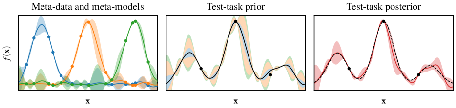
Figure 1: Illustration of ScaML-GP. We train individual GPs per meta-task (left), which combine with the task kernel $k_{t}$ and the task-weights $w_{m}$ to form the test-task prior. The HPs are inferred via MAP-inference to obtain the figure in the middle, where the shaded colors correspond to the meta-tasks contribution to the standard deviation. The posterior can then be obtained by conditioning the test-task prior distribution on $\mathcal{D}_{t}$ via 7 (right). Notice the decreased uncertainty estimate of the test posterior at the location of the meta-data.

Following Theorem 1 we can model each meta-task $m$ with an individual GP based on a kernel $k_{m}$. The resulting prior distribution of the test-task $f_{t}$ is a GP given by the weighted sum of meta-task posteriors according to 6. ScaML-GP thus models a full joint distribution over tasks and yields a prior on the test function that can be conditioned on $\mathcal{D}_{t}$ through 7 in order to obtain the test-task posterior

$$p(f_{t}\mid\mathbf{x},\mathcal{D}_{m},\mathcal{D}_{t})=\mathcal{N}\left(\mu_{t}(x),\Sigma_{t}(\mathbf{x},\mathbf{x})\right)$$ (7)

based on the prior mean and kernel from Theorem 1. Next to enabling a full Bayesian treatment of uncertainty, this also allows us to determine the meta-task weights $w_{m}$ by maximizing the likelihood. In light of Theorem 1, ScaML-GP reduces the complexity of the original MTGP from cubic in the total number of points to linear in the number of tasks. We achieve this solely by enforcing Assumptions 1 and 2 and without introducing numerical approximations. We illustrate the inner workings of ScaML-GP in Figure 1.

Likelihood optimization

So far we have assumed the HPs $\theta_{m}$ of the meta-task kernels $k_{m}$, and the test-task HPs $\theta_{t}$, which contain the parameters of $k_{t}$ and the weights $w_{m}$, to be given. In practice, they are inferred from the data $\mathcal{D}_{1:M}$ and $\mathcal{D}_{t}$. Naive evaluation of the likelihood of the joint task model in 5 is expensive, $O((N_{t}+M\overline{N}_{m})^{3})$ with $\overline{N}_{m}=\max_{m\in\mathcal{M}}N_{m}$, since it depends on all data. However, any model that complies with Assumption 1 is scalable in $M$ since

$$\log p\left(\mathbf{y}_{t},\mathbf{y}_{1:M}\mid\mathbf{X}_{t},\mathbf{X}_{1:M},\theta_{t},\theta_{1:M}\right)=$$ (8)

$$\log p\left(\mathbf{y}_{t}\mid\mathcal{D}_{1:M},\mathbf{X}_{t},\theta_{t},\theta_{1:M}\right)+\sum_{m\in\mathcal{M}}\log p\left(\mathbf{y}_{m}\mid\mathbf{X}_{m},\theta_{m}\right).$$

The second term is the per-meta-task likelihood that can be computed at cost $O(MN_{m}^{3})$, while the first is the likelihood under the test-task prior given by Theorem 1. Given the already inverted meta-task kernel matrices, computing the posterior meta-task covariances at test-task points $\mathbf{X}_{t}$ is of complexity $O(M(N_{t}^{2}\overline{N}_{m}+N_{t}\overline{N}_{m}^{2}))$. Together with the resulting test-task likelihood, $O(N_{t}^{3})$, this yields a total complexity of $O(M(\overline{N}_{m}^{3}+N_{t}^{2}\overline{N}_{m}+N_{t}\overline{N}_{m}^{2})+N_{t}^{3})$, which is linear in the number of meta-tasks $M$ and thus enables scalable optimization.

In practice, the number of test parameters in $\mathbf{X}_{t}$ is usually smaller than the available meta-data since the meta-prior already contains significant information. This leads to a weak dependence between the meta-model parameters $\theta_{m}$ and the test data $\mathbf{y}_{t}$. This is especially true for ScaML-GP, since the marginal per-task model only depends on $k_{m}$ and is thus independent of $\theta_{t}$. We therefore suggest to modularize ScaML-GP by assuming conditional independence between $\theta_{m}$ and $\mathcal{D}_{t}$ (Bayarri et al., 2009):

Assumption 3.

For all meta-tasks ${m\in\mathcal{M}}$, we have ${p\left(\theta_{m}\mid\mathcal{D}_{m},\mathcal{D}_{t}\right)=p\left(\theta_{m}\mid\mathcal{D}_{m}\right)}$.

Assumption 3 allows us to infer the meta-task HPs $\theta_{1:M}$ independently of the test-task HPs $\theta_{t}$. Thus, we can optimize the meta-task GPs in parallel based only on their individual data, $\theta_{m}^{\star}=\operatorname*{arg\,max}_{\theta_{m}}\log p(\mathbf{y}_{m}\mid\mathbf{X}_{m},\theta_{m})$. Afterwards, we compute and cache the meta-task GP posterior mean $\mu_{m}(\mathbf{X}_{t})$ and covariance matrix $\Sigma_{m}(\mathbf{X}_{t},\mathbf{X}_{t})$. Since the test-task prior in 6 depends on these quantities and not on $\theta_{t}$ due to Assumption 3, we can optimize the test-task likelihood,

$$\theta_{t}^{\star}=\operatorname*{arg\,max}_{\theta_{t}}\log p\left(\mathbf{y}_{t}\mid\mathcal{D}_{1:M},\mathbf{X}_{t},\theta_{t},\theta_{1:M}^{\star}\right),$$ (9)

at cost of only $O(MN_{t}^{2}+N_{t}^{3})$, which is cheap to evaluate. Together, this enables scalable meta-learning with Gaussian processes (ScaML-GP) and we use this simplification in our experiments. We summarize the algorithm in Algorithm 1.

Algorithm 1 ScaML-GP

1:  Input: meta-data $\mathcal{D}_{1:M}=\cup_{m\in\mathcal{M}}\mathcal{D}_{m}$

2:  Train individual GP models per meta-task and optimize $\theta_{m}$

3:  Construct the test-task prior as in 6, and cache $\mu_{m}(\mathbf{X}_{t})$ and $\Sigma_{m}(\mathbf{X}_{t},\mathbf{X}_{t})$.

4:  Optimize the test-task HPs $\theta_{t}$ as in 9

5:  Condition the prior on $\mathcal{D}_{t}$ as in 7 to obtain the posterior distribution for $f_{t}$

Discussion and limitations

Theorem 1 provides a scalable and structured way to distill meta-information into a prior for a test-task GP. The key component for this is Assumption 2, which assumes an additive model. While these models reflect many real-world situations, more flexible meta-learning models based on neural networks are in principle able to learn more complex relationships between the meta- and test-tasks. However, by relaxing the model assumptions these methods also require significantly more data. Thus ScaML-GP is most suited when the amount of data per task is relatively scarce. While the overall approach scales linearly with the number of meta-tasks and enables parallel optimization, each model is still a standard Gaussian process, which scales cubically in the number of points per task. For large number of data points per task, $N_{m}$ or $N_{t}$, the modular nature of ScaML-GP allows for full scalability in the number of points by employing scalable approximations for the task GPs (Lázaro-Gredilla et al., 2010). While an interesting direction, we focus on closed-form inference here and leave the exploration of full scalability for future work.

5 Experiments

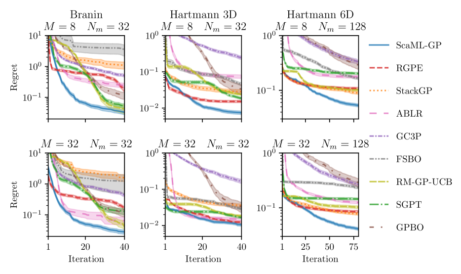
Figure 2: Experimental results on the synthetic benchmarks for two different meta-data configurations: $M=8$ and $32$ meta-tasks in the top and bottom row, respectively. The meta-data are sampled uniformly at random and contain $N_{m}=32$ points per meta-task for Branin and Hartmann 3D, and 128 for Hartmann 6D, respectively. ScaML-GP consistently achieves the lowest simple regret across all tasks. We provide a more detailed analysis on the effect of $M$ and $N_{m}$ on the performance in Figure 3.

We evaluate our method (ScaML-GP) on several optimization problems against the following baselines: standard GP-based BO (GPBO) without any meta-data, RGPE (Feurer et al., 2018) and SGPT (Wistuba et al., 2018), both of which model the test function as a weighted sum of the predictions of all task GPs, the method by Golovin et al. (2017), which we dub StackGP, since it trains a vertical stack of GPs and the posterior mean function of each GP is used as the prior mean function of the next GP, ABLR (Perrone et al., 2018), where Bayesian linear regression is performed on the deep features learned from the meta-data, RM-GP-UCB (Dai et al., 2022), where the acquisition function is a weighted sum of individual acquisition functions of each model (see Section C.4 for implementation details), FSBO (Wistuba and Grabocka, 2021), which is an extension of MAML to GPs, and GC3P (Salinas et al., 2020) in which a Gaussian Copula regression with a parametric prior are used to scale to large data. We implement the models and run BO using BoTorch (Balandat et al., 2020) and provide details on the experimental setup in Appendix C.

5.1 Synthetic Benchmarks

Our synthetic-benchmark consists of conventional benchmark functions, where we place priors on some of their parameters. We consider the two-dimensional Branin, three-dimensional Hartmann 3D, and six-dimensional Hartmann 6D and provide details on the function families and the priors in Section C.6. Note that these are generic meta-learning benchmarks that are not designed to fulfill Assumptions 1, 2 and 3. We evaluate performance based on the simple regret ${r=\max_{\mathbf{x}\in D}f_{t}(x)-\max_{n\leq N_{t}}f_{t}(\mathbf{x}_{n})\geq 0}$, which is the difference between the true optimum and the best function value obtained during the current optimization run. For each benchmark, we conduct 128 independent runs and report mean and standard error in our figures. For each run, the meta-data is consistent across all baselines for comparability.

The performance of the different baselines on the synthetic benchmarks for $M=8$ (top row) and $M=32$ (bottom row) meta-tasks is visualized in Figure 2. The regret of GPBO converges in about 40 iterations for the two- and three-dimensional benchmarks and needs more than 80 iterations for Hartmann 6D. As expected, most meta-learning baselines converge faster than GPBO, since they can leverage additional information. In general, different baselines excel in different data-regimes. For instance, RGPE is among the best for the Hartmann families, while ABLR provides competitive performance on Branin after about ten iterations. In contrast, ScaML-GP, consistently demonstrates fast task adaptation and achieves the lowest regret at the end of each experiment compared to all baseline methods. This demonstrates that there is an advantage to employing a joint Bayesian model across tasks. For ABLR, we can see that performance improves significantly as we increase the number of meta-tasks, and thus the overall amount of meta-data, in the bottom row. In contrast, ScaML-GP performs consistently across both domains, which aligns with the findings of Tighineanu et al. (2022) that GP-based methods have an advantage when meta-data is scarce.

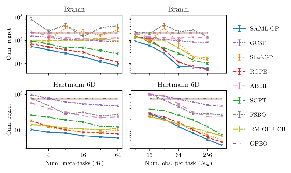
Figure 3: Summary of the performance of the meta-learning baselines on two synthetic benchmarks, Branin (top) and Hartmann 6D (bottom), as a function of the number of meta-tasks $M$ for a fixed number of points per task ($N_{m}=32$ and 128 for Branin and Hartmann 6D, respectively) on the left side, and as a function of the number of points per task $N_{m}$ for a fixed number of $M=8$ meta-tasks on the right side. Each data point denotes the mean and standard error of the cumulative regret at the end of the optimization. ScaML-GP consistently achieves the lowest cumulative regret across all data domains, which indicates that it is well suited for the low-data domain, but can also effectively scale to many tasks.

Ablation on meta-data

We now study in detail how the performance of all methods depends on the amount of meta-data. In particular, we independently vary the amount of meta-data per task and the number of meta-tasks on the Branin and Hartmann 6D tasks. As we increase the number of tasks we get better coverage of the task distribution, whereas increasing the number of observations per task allows us to learn more about each individual meta-task. We present a condensed version of this ablation study in Figure 3, where we plot the cumulative regret at the end of the optimization. More information including the simple regret plots are available in Appendix D. As in Figure 2, we observe that most meta-learning baselines outperform standard GPBO throughout the ablation range. Similarly, as we increase the amount of meta-data, meta-learning methods generally improve performance since they have more information about the task family. The exception to this rule is StackGP, which unlike other methods does not scale to many tasks $M$ (top left), since it builds a hierarchical sequential model based on mean functions only and is thus not able to convey uncertainty information effectively. This effect is most pronounced for Branin, where the the optimum of different tasks varies continuously, while for Hartmann 6D they are restricted to four discrete locations. For Branin we can observe in the top-right figure that starting at about a hundred observations per task performance starts to saturate, since that is sufficient information to train confident meta-task models. Overall ScaML-GP outperforms other baselines across all data domains. While other methods can match the performance in some settings, ScaML-GP performs consistently well across all settings.

5.2 HPO Benchmarks

We compare all methods on a set of tasks where we have to optimize the HPs of machine-learning models. Each benchmark considers a specific machine learning model and a task consists of adapting the model’s HPs in order to minimize the expected loss on a given dataset across several random seeds. To facilitate fast exploration, we base our study on the tabular benchmarks available as part of the HPOBench library (Eggensperger et al., 2021). For each task, it provides a lookup table that maps HP configurations to the corresponding loss. For BO, we restrict the parameter space of each benchmark to contain only the discrete values in the lookup table. We consider HP optimization tasks for a support-vector-machine (SVM) model, logistic regression (LR), XGBoost model (XGB), random forest (RF), and neural-network (MLP) model. We randomly assign one of the tasks to be our test function for a single independent run, while the remaining tasks are used for meta-learning. We sub-sample the meta-data to $N_{m}=64$ points per task for the two-dimensional SVM and LR, and to $N_{m}=128$ points per task for the four-dimensional XGB and RF, and five-dimensional MLP benchmarks. In addition, we provide results on the tabular FC-Net benchmarks Slice Localization, Protein Structure, Naval Propulsion, and Parkinson’s Telemonitoring (Eggensperger et al., 2021). For each of the four, we use one as test task and the other three as meta-tasks. We report the mean simple regret together with the standard error of the mean computed over 256 independent runs. We provide further details about the HPO benchmarks in Section C.7.

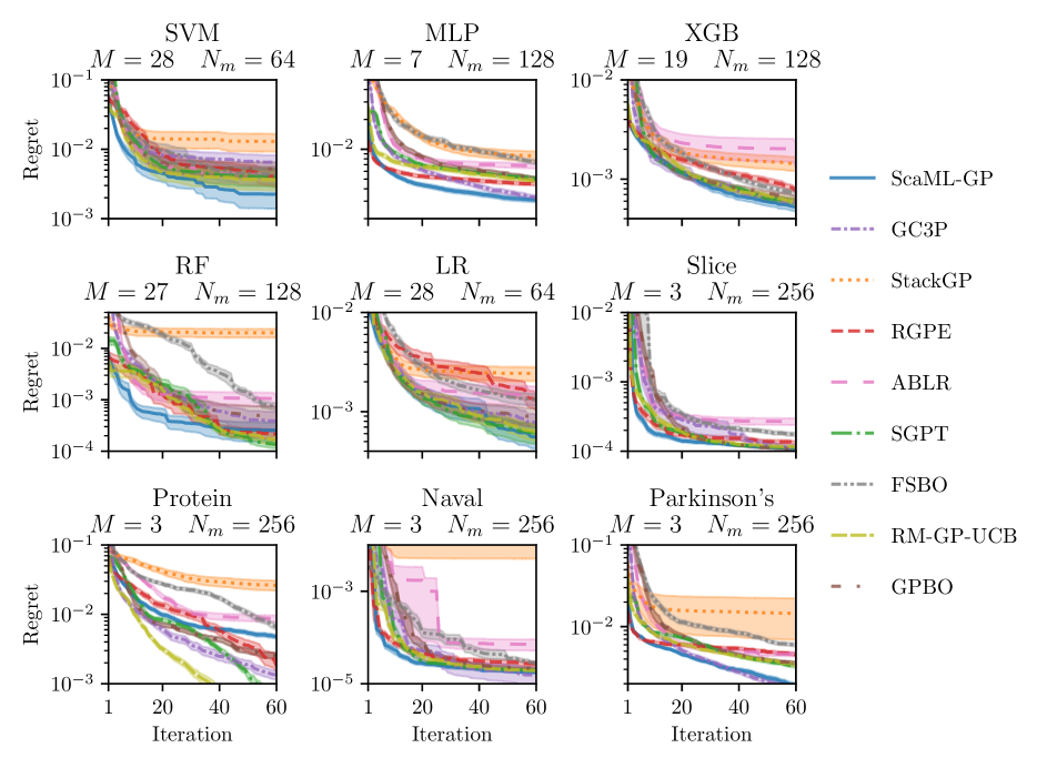
Figure 4: Experimental results on different hyperparameter optimization problems for machine learning models from five tabular HPO benchmarks (SVN, MLP, XGB, RF, and LR), as well four tabular FC-Net benchmarks (Slice, Protein, Naval, and Parkinson’s). For each model, training runs on different datasets are used as meta-data with $N_{m}$ points per each of the $M$ meta-tasks to better inform hyperparameter choices on a new test-task dataset. ScaML-GP is either the best or joint-best baseline on all benchmarks except the FC-Net Protein.

In Figure 4 we show a comparison of the methods on all nine HPO benchmarks. Most meta-learning baselines successfully leverage the meta-data and achieve smaller regrets than GPBO early in the optimization. Towards the end of the optimization process, some baselines perform worse than GPBO, which is most likely related to the inductive bias in the meta-data. Crucially, the threshold from better to worse varies among benchmarks, e.g., about ten iterations for XGB and thirty for RF. In practice, this threshold is not known to the user and makes it challenging to estimate the iteration budget or be confident in superior performance for a fixed budget. In contrast, ScaML-GP is consistently competitive across all benchmarks in all optimization stages. This evidence is in line with the performance on the synthetic benchmarks in Figure 2. The exception where ScaML-GP performs subpar is the FC-Net Protein benchmark. Our analysis indicates that this is because Assumption 2 is grossly violated such that no linear combination of the three meta-task models yields a useful test-task prior, see Section C.3 for a detailed discussion. We believe that the strong overall performance of ScaML-GP is a result of the principled Bayesian approach together with assumptions that enable task scalability.

6 Conclusion

We have presented ScaML-GP, a scalable GP for meta-learning. It is a specific instance of a multi-task GP model in 2, but based on explicit assumptions on the model structure in order to obtain a method that is scalable in the number of meta-tasks $M$. In particular, our test-prior is a weighted linear combination of the per-meta-task GP posterior distributions together with a residual model that accounts for test-functions that cannot be explained through the meta-data. In contrast to ensemble methods like RGPE, this joint Bayesian model allows us to use maximum likelihood optimization in order to determine the weights. Moreover, we showed that hyperparameter inference in ScaML-GP can be parallelized in order to enable efficient learning. Finally, we compared our method against a set of GP-based and neural-network-based meta-learning methods. ScaML-GP consistently performed well across various benchmarks and number of meta-tasks.

Overview

In the appendix we provide the detailed proofs for all claims in the paper, complexity analysis, ablation studies, and details on experiments. An overview is shown below.

Appendix A Kernel Properties

We start by showing that for a single meta-task, the coregionalization is indeed positive semi-definite.

Lemma 2.

For any $w_{m}\in\mathbb{R}$

$$\mathbf{W}_{m}=\begin{bmatrix}1&w_{m}\\ w_{m}&w_{m}^{2}\end{bmatrix}$$ (10)

is positive semi-definite.

Proof.

Let $\mathbf{x}=(x_{1},x_{2})\in\mathbb{R}^{2}$, then $\mathbf{x}^{T}\mathbf{W}_{m}\mathbf{x}=x_{1}^{2}+2w_{m}x_{1}x_{2}+w_{m}^{2}x_{2}^{2}=(x_{1}+w_{m}x_{2})^{2}\geq 0$, i.e. $\mathbf{W}_{m}$ is positive semi-definite. ∎

Lemma 3.

For any $w_{m}\in\mathbb{R}$ the coregionalization matrices specified by 4 are positive semi-definite.

Proof.

Each matrix $\mathbf{W}_{m}$ has the same form as in Lemma 2, but with additional zero rows and columns added. That is, from Lemma 2 for any $\mathbf{x}=(\mathbf{x}_{1},\dots,\mathbf{x}_{M+1})\in\mathbb{R}^{M+1}$ we have

$$\mathbf{x}^{T}\mathbf{W}_{m}\mathbf{x} =(x_{m},x_{M+1})^{T}\begin{bmatrix}1&w_{m}\\ w_{m}&w_{m}^{2}\end{bmatrix}(x_{m},x_{M+1})\geq 0.$$ (11)

According to 4, we have

$$\mathbf{W}_{t}=\begin{bmatrix}\mathbf{0}&\mathbf{0}\\ \mathbf{0}&1\end{bmatrix}\in\mathbb{R}^{(M+1)\times(M+1)},$$

from which we obtain $\mathbf{x}^{\mathrm{T}}\mathbf{W}_{t}\mathbf{x}=\mathbf{x}_{M+1}^{2}\geq 0$ for any $\mathbf{x}=(\mathbf{x}_{1},\dots,\mathbf{x}_{M+1})\in\mathbb{R}^{M+1}$. ∎

See 1

Proof.

We begin by showing that the coregionalization matrices in 4 are uniquely defined by Assumptions 1 and 2. To see this, we first collect all terms in 2:

$$k((\mathbf{x},m),(\mathbf{x}^{\prime},m)) =\mathrm{Cov}\left(f_{m}(x),f_{m}(x^{\prime})\right)=k_{m}(x,x^{\prime}),\quad\text{(\lx@cref{creftype~refnum}{as:independent_sources})}$$ (12)

$$k((\mathbf{x},m),(\mathbf{x}^{\prime},m^{\prime}\neq m)) =\mathrm{Cov}\left(f_{m}(x),f_{m^{\prime}}(x^{\prime})\right)=0,\quad\text{(\lx@cref{creftype~refnum}{as:independent_sources})}$$ (13)

$$k((\mathbf{x},m),(\mathbf{x}^{\prime},t)) =\mathrm{Cov}\left(f_{m}(x),f_{t}(x^{\prime})\right)$$

$$=\mathrm{Cov}\left(f_{m}(\mathbf{x}),\tilde{f}_{t}+\sum_{m^{\prime}\in\mathcal{M}}\tilde{f}_{m^{\prime}}(\mathbf{x}^{\prime})\right)\quad\text{(\lx@cref{creftype~refnum}{as:strong_correlation})}$$

$$=\mathrm{Cov}\left(f_{m}(\mathbf{x}),\sum_{m^{\prime}\in\mathcal{M}}\tilde{f}_{m^{\prime}}(\mathbf{x}^{\prime})\right)\quad\text{(\lx@cref{creftype~refnum}{as:strong_correlation})}$$

The perfect (anti)correlation $\mathrm{Corr}\left(f_{m}(\mathbf{x}),\tilde{f}_{m}(\mathbf{x})\right)=\pm 1$ in Assumption 2 implies that $\tilde{f}_{m}(\mathbf{x})=w_{m}f_{m}(\mathbf{x})+c$ with $w_{m},c\in\mathbb{R}$. Hence $\mathrm{Cov}\left(f_{m}(\mathbf{x}),\tilde{f}_{m^{\prime}}(\mathbf{x}^{\prime})\right)=w_{m^{\prime}}\mathrm{Cov}\left(f_{m}(\mathbf{x}),f_{m^{\prime}}(\mathbf{x}^{\prime})\right)$. Together with Assumption 1 this becomes $\mathrm{Cov}\left(f_{m}(\mathbf{x}),\tilde{f}_{m^{\prime}}(\mathbf{x}^{\prime})\right)=\delta_{m,m^{\prime}}w_{m}k_{m}(x,x^{\prime})$. Using that the covariance is bilinear it follows that

$$k((\mathbf{x},m),(\mathbf{x}^{\prime},t)) =\sum_{m^{\prime}\in\mathcal{M}}\mathrm{Cov}\left(f_{m}(\mathbf{x}),\tilde{f}_{m^{\prime}}(\mathbf{x}^{\prime})\right)=w_{m}k_{m}(x,x^{\prime}).$$ (14)

Finally, we have

$$k((\mathbf{x},t),(\mathbf{x}^{\prime},t)) =\mathrm{Cov}\left(f_{t}(x),f_{t}(x^{\prime})\right)$$

$$=k_{t}(x,x^{\prime})+\sum_{m\in\mathcal{M}}\mathrm{Cov}\left(f_{t}(\mathbf{x}),\tilde{f}_{m}(\mathbf{x}^{\prime})\right)\quad\text{(\lx@cref{creftype~refnum}{as:strong_correlation} and }k_{t}(x,x^{\prime})=\mathrm{Cov}\left(f_{t}(x),\tilde{f}_{t}(x^{\prime})\right))$$

$$=k_{t}(x,x^{\prime})+\sum_{m\in\mathcal{M}}\mathrm{Cov}\left(\tilde{f}_{t}+\sum_{m^{\prime}\in\mathcal{M}}\tilde{f}_{m^{\prime}}(\mathbf{x}),\tilde{f}_{m}(\mathbf{x}^{\prime})\right)\quad\text{(\lx@cref{creftype~refnum}{as:strong_correlation})}$$

$$=k_{t}(x,x^{\prime})+\sum_{m\in\mathcal{M}}\mathrm{Cov}\left(\tilde{f}_{m}(\mathbf{x}),\tilde{f}_{m}(\mathbf{x}^{\prime})\right)\quad\text{(\lx@cref{creftype~refnum}{as:independent_sources}, \lx@cref{creftype~refnum}{as:strong_correlation})}$$

Since $\tilde{f}_{m}(\mathbf{x})=w_{m}f_{m}(\mathbf{x})+c$ as shown above and using bilinearity of the covariance, we have

$$k((\mathbf{x},t),(\mathbf{x}^{\prime},t)) =k_{t}(x,x^{\prime})+\sum_{m\in\mathcal{M}}w_{m}^{2}k_{m}(x,x^{\prime}).$$ (16)

By collecting the coefficients corresponding to the $k_{m}$, $k_{t}$ we obtain the coregionalization matrices.

Further, from Lemma 3 and (Álvarez et al., 2012) we obtain that $k_{\mathrm{ScaML}}^{\mathrm{joint}}$ is positive semi-definite as a linear combination of positive semi-definite coregionalization matrices and kernels. That is, 4 yield a valid multi-task kernel.

Finally, from the definition of the Dirac-delta and $g_{m}(\nu)$, we have

$$\delta_{\nu=t}\delta_{\nu^{\prime}=t} =\begin{cases}1&\text{if }\nu=\nu^{\prime}=t,\\ 0&\text{else,}\\ \end{cases} g_{m}(\nu)g_{m}(\nu^{\prime})=\begin{cases}w_{m}^{2}&\text{if }\nu=\nu^{\prime}=t,\\ w_{m}&\text{if }\nu=m,\nu^{\prime}=t,\text{or }\nu=t,\nu^{\prime}=m,\\ 1&\text{if }\nu=\nu^{\prime}=m,\\ 0&\text{else.}\end{cases}$$ (17)

The statement from the Lemma follows from $\delta_{\nu=t}\delta_{\nu^{\prime}=t}=[\mathbf{W}_{t}]_{(\nu,\nu^{\prime})},\,g_{m}(\nu)g_{m}(\nu^{\prime})=[\mathbf{W}_{m}]_{(\nu,\nu^{\prime})}$ for all $\nu,\nu^{\prime}$ and the fact that 4 yield a valid kernel. ∎

See 1

Proof.

According to 5, the joint prior model for the meta-observations $\mathbf{y}_{\mathrm{meta}}=(\mathbf{y}_{1},\dots,\mathbf{y}_{\mathrm{meta}})$ and the test-task function value at a query point $\mathbf{x}$ given by

$$\begin{bmatrix}\mathbf{y}_{\mathrm{meta}}\\ f_{t}(\mathbf{x})\end{bmatrix}\sim\mathcal{N}\left(\mathbf{0},\begin{bmatrix}\mathbf{K}_{\mathrm{meta}}&\mathbf{k}_{\mathrm{meta}}\\ \mathbf{k}_{\mathrm{meta}}^{\mathrm{T}}&\mathbf{K}_{t}\end{bmatrix}\right)$$ (18)

where

$$\mathbf{K}_{\mathrm{meta}} =\mathrm{diag}\big{(}k_{1}(\mathbf{X}_{1},\mathbf{X}_{1})+\sigma_{1}^{2}\mathbf{I},\dots,k_{M}(\mathbf{X}_{M},\mathbf{X}_{M})+\sigma_{M}^{2}\mathbf{I}\big{)},$$

$$\mathbf{k}_{\mathrm{meta}} =\big{(}w_{1}k_{1}(\mathbf{X}_{1},\mathbf{x}),\dots,w_{M}k_{M}(\mathbf{X}_{M},\mathbf{x})\big{)},$$

$$\mathbf{K}_{t} =\big{(}k_{t}(\mathbf{x},\mathbf{x})+\sum_{m}w_{m}^{2}k_{m}(\mathbf{x},\mathbf{x})\big{)}.$$

Conditioning on the meta-data $\mathcal{D}_{1:M}$ yields

$$p(f_{t}\mid\mathcal{D}_{1:M},\mathbf{x})=\mathcal{N}\left(m_{\mathrm{ScaML}}(\mathbf{x}),\Sigma_{\mathrm{ScaML}}(\mathbf{x},\mathbf{x})\right),$$ (19)

where the test-task prior mean $m_{\mathrm{ScaML}}$ and covariance $\Sigma$ are given by the standard Gaussian conditioning rules

$$m_{\mathrm{ScaML}}(\mathbf{x}) =\mathbf{k}_{\mathrm{meta}}^{\mathrm{T}}\mathbf{K}_{\mathrm{meta}}^{-1}\mathbf{y}_{\mathrm{meta}},$$

$$\Sigma_{\mathrm{ScaML}}(\mathbf{x},\mathbf{x}) =\mathbf{K}_{t}-\mathbf{k}_{\mathrm{meta}}^{\mathrm{T}}\mathbf{K}_{\mathrm{meta}}^{-1}\mathbf{k}_{\mathrm{meta}}.$$

Now since $\mathbf{K}_{\mathrm{meta}}$ is block-diagonal, we have

$$\mathbf{K}_{\mathrm{meta}}^{-1}=\mathrm{diag}\left((k_{1}(\mathbf{X}_{1},\mathbf{X}_{1})+\sigma_{1}^{2}\mathbf{I})^{-1},\dots,(k_{M}(\mathbf{X}_{M},\mathbf{X}_{M})+\sigma_{M}^{2}\mathbf{I})^{-1}\right),$$

so that

$$m_{\mathrm{ScaML}}(\mathbf{x}) =\sum_{m}w_{m}k_{m}(\mathbf{x},\mathbf{X}_{m})(k_{m}(\mathbf{X}_{m},\mathbf{X}_{m})+\sigma_{m}^{2}\mathbf{I})^{-1}\mathbf{y}_{m},$$

$$=\sum_{m}w_{m}\mu_{m}(\mathbf{x}),$$

where $\mu_{m}(\mathbf{x})$ is the per meta-task posterior mean after conditioning on the corresponding data $\mathcal{D}_{m}$. Similarly, for the covariance we have

$$\Sigma_{\mathrm{ScaML}}(\mathbf{x},\mathbf{x}) =\mathbf{K}_{t}-\mathbf{k}_{\mathrm{meta}}^{\mathrm{T}}\mathbf{K}_{\mathrm{meta}}^{-1}\mathbf{k}_{\mathrm{meta}},$$

$$=k_{t}(\mathbf{x},\mathbf{x})+\sum_{m}w_{m}^{2}k_{m}(\mathbf{x},\mathbf{x})-\sum_{m}w_{m}k_{m}(\mathbf{x},\mathbf{X}_{m})(k_{m}(\mathbf{X}_{m},\mathbf{X}_{m})+\sigma_{m}^{2}\mathbf{I})^{-1}w_{m}k_{m}(\mathbf{X}_{m},\mathbf{x}),$$

$$=k_{t}(\mathbf{x},\mathbf{x})+\sum_{m}w_{m}^{2}k_{m}(\mathbf{x},\mathbf{x})-w_{m}^{2}k_{m}(\mathbf{x},\mathbf{X}_{m})(k_{m}(\mathbf{X}_{m},\mathbf{X}_{m})+\sigma_{m}^{2}\mathbf{I})^{-1}k_{m}(\mathbf{X}_{m},\mathbf{x}),$$

$$=k_{t}(\mathbf{x},\mathbf{x})+\sum_{m}w_{m}^{2}\big{(}k_{m}(\mathbf{x},\mathbf{x})-k_{m}(\mathbf{x},\mathbf{X}_{m})(k_{m}(\mathbf{X}_{m},\mathbf{X}_{m})+\sigma_{m}^{2}\mathbf{I})^{-1}k_{m}(\mathbf{X}_{m},\mathbf{x})\big{)},$$

$$=k_{t}(\mathbf{x},\mathbf{x})+\sum_{m}w_{m}^{2}\Sigma_{m}(\mathbf{x},\mathbf{x}),$$

where $\Sigma_{m}$ is the corresponding per meta-task posterior covariance. ∎

Appendix B Complexity Analysis

Here we analyze the computational complexity of evaluating the likelihood of the test-data under the prior 7. We break this down into the complexities for evaluating the posterior mean and the posterior covariance of the test-task.

As an intermediate step, the kernel matrices of the meta-tasks need to be inverted, which is of complexity $O(\sum_{m\in\mathcal{M}}N_{m}^{3})$. This only needs to happen once and then those inverted matrices can be cached.

To construct the test-task prior we need to evaluate each meta-task posterior mean at all x-values in the test-task dataset $\mathbf{X}_{t}$. Given the cached kernel matrices each evaluation costs $O(N_{m}^{2})$ multiplications resulting in a complexity of $O(N_{t}\sum_{m\in\mathcal{M}}N_{m}^{2})$. In addition, we also need to evaluate the posterior covariance at the same parameters. In contrast to the posterior mean computation, evaluating the covariance matrix at all parameters $\mathbf{X}_{t}$ jointly results in a lower computational complexity than isolated forward calculation of all $N_{t}^{2}$ entries. The corresponding matrix multiplication in 7 is of order $O(N_{t}^{2}N_{m}+N_{t}N_{m}^{2})$. The complexities for all meta-tasks add up to $O(N_{t}^{2}\sum_{m\in\mathcal{M}}N_{m}+N_{t}\sum_{m\in\mathcal{M}}N_{m}^{2})$.

Further in the likelihood we also need to evaluate the test-task posterior at the test-task data points. This requires to evaluate 7 and is dominated by the inversion of the test-task kernel matrix, which is of order $O(N_{t}^{3})$.

Summarizing the complexity of evaluating the likelihood is given by the complexity of inverting the meta-task kernel matrices $O(\sum_{m\in\mathcal{M}}N_{m}^{3})$ once and the reoccurring cost of constructing the test-task prior and evaluating the test-task posterior, which is of order $O(N_{t}^{2}\sum_{m\in\mathcal{M}}N_{m}+N_{t}\sum_{m\in\mathcal{M}}N_{m}^{2}+N_{t}^{3})$.

As mentioned in Section 4, we can use Assumption 3 in order to cache intermediate results in order to further reduce complexity.

Appendix C Details on Experiments

In all experiments we use BoTorch’s implementation of Upper Confidence Bound acquisition function with the exploration coefficient $\beta^{1/2}=3$. For the experiments on the synthetic benchmarks, the meta and test functions are sampled randomly from a function family, while the meta-data parameters are sampled uniformly from the task’s domain $D$. We optimize the test function from scratch without initial samples. We add i.i.d. zero-mean Gaussian observational noise during the data generation with a standard deviation of 1.0 for Branin and 0.1 for Hartmann 3D and 6D. This amount of noise corresponds to about one percent of the output scale of the benchmark in the search space.

We implement all GP models using the squared-exponential kernel with automatic relevance determination. The GP hyperparameters are optimized at each BO iteration by maximizing the likelihood of the observed data using the L-BFGS-B optimizer with 5 initial guesses. These guesses are sampled from the prior of the hyperparameter. We normalize the GP data as explained in Section C.1. All other details regarding training and prediction are kept fixed to BoTorch’s defaults (Balandat et al., 2020).

C.1 Data Normalization

We follow the common practice and normalize the GP data. The search space of the input parameters is rescaled to the unit hypercube in the data pre-processing pipeline. The observations are normalized to zero-mean unit-variance individually for each GP. An exception is ScaML-GP’s test-task GP for which observations, $\mathbf{y}_{t}$, are normalized with respect to the mean and variance of $\mathbf{y}_{t}\cup\mathbf{y}_{1:M}$. We prefer this strategy over normalizing solely with respect to $\mathbf{y}_{t}$ whose statistics are volatile at the start of the optimization.

C.2 Implementation Details of ScaML-GP

We implement ScaML-GP according to Algorithm 1.

1. We train individual GP models on the data of each meta-task and independently optimize the marginal likelihoods. These meta-data are individually normalized to zero-mean unit-variance.

2. We construct the test-task prior as in Theorem 1 by summing over the posteriors of the GP of each meta-task. Assumption 3 allows us to cache $\mu_{m}(\mathbf{X}_{t})$ and $\Sigma_{m}(\mathbf{X}_{t},\mathbf{X}_{t})$.

3. We optimize the hyperparameters, $\theta_{t}$, of the test-task GP. For this we normalize $\mathbf{y}_{t}$ as explained in Section C.1. This joint normalization implies that $\mathbf{y}_{t}$ generally have a non-zero mean and non-unit variance.

4. We condition the test-task GP on $\mathcal{D}_{t}$. Since $\mathbf{y}_{t}$ are not standardized, the optimum hyperparameters of the test-task kernel, $k_{t}$, are distributed differently than those of standard GPs. We consider this when choosing prior distributions for the GP hyperparameters in Section C.5.

C.3 Importance of Satisfying the Assumptions of ScaML-GP in Practice

ScaML-GP is a modular and flexible method for meta-learning that is scalable in the number of tasks. ScaML-GP can be applied to a wide variety of meta-learning settings as demonstrated in Section 5 and is designed to excel in the regime of relatively little amount of data per meta-task.

While the assumptions of ScaML-GP may seem restrictive, Assumptions 1, 2 and 3, empirical results clearly demonstrate that ScaML-GP performs excellently in most scenarios. This is because ScaML-GP has built-in mechanisms that can easily handle violations of these assumptions. In particular,

• Assumption 1, independence of the prior distributions of meta-task models, is clearly violated in most use cases. However, they do not limit learning as long as each meta-task contains sufficient data allowing for a probabilistic description of the meta-task function. This amount of data can be surprisingly little for GPs as seen in Figure 3 – as little as 16 points in a six-dimensional search space are enough to significantly improve over GPBO and other meta-learning baselines.

• Assumption 2, perfect correlation between meta-task models and components of the test-task models, is likewise violated in most use cases. ScaML-GP can easily handle such violations via the test-task component of the kernel, $k_{t}(\mathbf{x},\mathbf{x}^{\prime})$ (see 6), which can learn arbitrary non-linear deviations from the prediction of the meta-task models. In the worst-case scenario in which no linear combination of meta-task functions is useful, ScaML-GP simply ignores the meta-data and optimizes the process from scratch using the test-task component of the kernel. Such an example can be seen in Figure 4 (FC-Net Protein benchmark).

• Assumption 3, independence between meta-task HPs, $\theta_{m}$, and test-task observations $\mathcal{D}_{t}$, is motivated by the meta-learning setting in which meta-data are abundant but test-data are scarce.

Only Assumption 1 is necessary for making our method scalable. Assumption 2 confers an explainable structure to the kernel and to the test-task prior in 6 but other choices are, in principle, also possible. Finally, Assumption 3 leads to a particularly efficient implementation of ScaML-GP.

C.4 Implementation Details of RM-GP-UCB

We implement RM-GP-UCB according to the UCB based algorithm in (Dai et al., 2022) with the following choices. For ease of implementation and to be consistent with other methods, we set the exploration coefficients to a constant value $\beta_{t}=\tau=3$. To ensure invariance of the acquisition function maximizer under a joint rescaling of all functions, we divide the bounds on the function gap $\bar{d}_{t,i}$ by the mean of the standard deviations across all meta-tasks before using them in the calculation of the weights $\nu_{t}$ and $\omega_{i}$. Finally, we set the hyperparameter $\delta=0.05$.

C.5 Choices of Prior Distributions and Constraints for GP Hyperparameters

In the following we discuss our choice of the prior distribution of the GP hyperparameters as well as the constraints we place on them.

Lengthscale

The prior of the lengthscale hyperparameter, $\theta_{l}$, is kept fixed to BoTorch’s default, $\theta_{l}\sim\Gamma(3,6)$, where $\Gamma$ denotes the Gamma distribution. This corresponds to a 5-95% quantile range of 0.14 – 1.05. Exception to this is the test-task kernel of StackGP and ScaML-GP, $k_{t}$, with $\log(\theta_{l})\sim\mathcal{N}(0.5,1.5)$ with a 5-95% quantile range of 0.14 – 19.44. With this broader distribution we introduce less inductive bias while keeping the risk of over-fitting low owing to the existence of an informative prior from the models of the meta-tasks. The lengthscale parameter is constrained to lie between $10^{-4}-10^{2}$ to avoid running into numerical issues.

Outputscale

The prior of the outputscale hyperparameter (signal variance), $\theta_{o}$, is also kept fixed to BoTorch’s default, ${\theta_{o}\sim\Gamma(2.0,0.15)}$ with a 5-95% quantile range of 2.4 – 31.8. Exception to this is the test-task kernel of ScaML-GP due to the different normalization strategy discussed in Section C.1. We choose a less biased distribution to accommodate this change in data normalization, $\log(\theta_{o})\sim\mathcal{N}(-2.0,3.0)$ with a 5-95% quantile range of $10^{-3}-18.8$. The outputscale parameter is constrained to lie between $10^{-4}-10^{2}$ to avoid running into numerical issues.

Observation noise

The prior of the observational-noise hyperparameter (noise variance), $\theta_{n}$, is set to $\log(\theta_{n})\sim\mathcal{N}(-8,2)$ with 5-95% quantile range of $1.25\cdot 10^{-5}-9\cdot 10^{-3}$. The noise parameter is constrained to lie between $10^{-8}-10^{-2}$ to avoid running into numerical issues.

Weights of ScaML-GP

We choose a generic prior distribution for the weights, ${w_{m}\sim\Gamma(1,1)}$, independently for each meta-task $m$. This distribution is flat and thus unbiased for $w_{m}\lesssim 1$, and decaying quickly for $w_{m}\gtrsim 1$. We constrain the weights to be strictly positive, $w_{m}>0$, implying that we only learn correlations and ignore anti-correlations.

C.6 Synthetic Benchmarks

The Branin Benchmark

The Branin function is a two-dimensional function with three global optima defined as

$$f(x_{1},x_{2};a,b,c,r,s,t)=a(x_{2}-bx_{1}^{2}+cx_{1}-r)+s(1-t)\cos(x_{1})+s,\quad x_{1}\in\left[-5,10\right],x_{2}\in\left[0,15\right]$$ (20)

We convert it to a meta-learning benchmark by choosing the following probability distributions for the parameters $(a,b,c,r,s,t)$:

$$a \sim\mathcal{U}(0.5,1.5),$$ (21)

$$b \sim\mathcal{U}(0.1,0.15),$$

$$c \sim\mathcal{U}(1,2),$$

$$r \sim\mathcal{U}(5,7),$$

$$s \sim\mathcal{U}(8,12),$$

$$t \sim\mathcal{U}(0.03,0.05).$$

The Branin meta-learning benchmark is thus defined over a six-dimensional uniform distribution. For generating the data of $n_{s}$ meta-tasks, we draw $n_{s}$ random tasks using 21, and sample a given number of parameters per task uniformly at random.

The Hartmann 3D Benchmark

The Hartmann 3D function is a sum of four three-dimensional Gaussian distributions and is defined by

$$f(\mathbf{x};\bm{\alpha})=-\sum_{i=1}^{4}\alpha_{i}\exp\left(-\sum_{j=1}^{3}A_{i,j}\left(x_{j}-P_{i,j}\right)^{2}\right),\quad\mathbf{x}\in\left[0,1\right]^{3},$$ (22)

with

$$\mathbf{A}=\begin{bmatrix}3.0&10&30\\ 0.1&10&35\\ 3.0&10&30\\ 0.1&10&35\end{bmatrix},\quad\mathbf{P}=10^{-4}\begin{bmatrix}3689&1170&2673\\ 4699&4387&7470\\ 1091&8732&5547\\ 381&5743&8828\end{bmatrix}.$$

The original Hartmann 3D function is given by $\bm{\alpha}=(1.0,1.2,3.0,3.2)^{T}$. In this paper, a family of functions is formed by choosing the following probability distributions for the parameters $\bm{\alpha}=(\alpha_{1},\alpha_{2},\alpha_{3},\alpha_{4})^{T}$:

$$\alpha_{1}\sim\mathcal{U}(1.00,1.02),\quad\alpha_{2}\sim\mathcal{U}(1.18,1.20),\quad\alpha_{3}\sim\mathcal{U}(2.8,3.0),\quad\alpha_{4}\sim\mathcal{U}(3.2,3.4).$$ (23)

The Hartmann 3D family therefore spans a four-dimensional uniform distribution. For generating the data of $M$ meta-tasks, we draw $M$ random tasks using 23, and sample a given number of parameters per task uniformly at random.

The Hartmann 6D Benchmark

The Hartmann 6D function is a sum of four six-dimensional Gaussian distributions with six local optima and one global optimum and is defined by

$$f(\mathbf{x};\bm{\alpha})=-\sum_{i=1}^{4}\alpha_{i}\exp\left(-\sum_{j=1}^{6}A_{i,j}\left(x_{j}-P_{i,j}\right)^{2}\right),\quad\mathbf{x}\in\left[0,1\right]^{6},$$ (24)

with

$$\begin{split}\mathbf{A}&=\hphantom{10^{-4}}\begin{bmatrix}10&3&17&3.5&1.7&8\\ 0.05&10&17&0.1&8&14\\ 3&3.5&1.7&10&17&8\\ 17&8&0.05&10&0.1&14\end{bmatrix},\\ \mathbf{P}&=10^{-4}\begin{bmatrix}1312&1696&5569&124&8283&5886\\ 2329&4135&8307&3736&1004&9991\\ 2348&1451&3522&2883&3047&6650\\ 4047&8828&8732&5743&1091&381\end{bmatrix}.\end{split}$$

The original Hartmann 6D function is given by $\bm{\alpha}=(1.0,1.2,3.0,3.2)^{T}$. We convert it to a meta-learning benchmark by placing the following probability distributions for $\bm{\alpha}=(\alpha_{1},\alpha_{2},\alpha_{3},\alpha_{4})^{T}$ based on the emukit (Paleyes et al., 2019) implementation:

$$\alpha_{1}\sim\mathcal{U}(1.00,1.02),\quad\alpha_{2}\sim\mathcal{U}(1.18,1.20),\quad\alpha_{3}\sim\mathcal{U}(2.8,3.0),\quad\alpha_{4}\sim\mathcal{U}(3.2,3.4).$$ (25)

The Hartmann 6D meta-learning benchmark is therefore defined over a four-dimensional uniform distribution. For generating the data of $M$ meta-data sets, we draw $M$ random tasks using 25, and sample a given number of parameters per meta-task uniformly at random.

C.7 Meta-Learning and Bayesian Optimization on Tabular Benchmarks

For the machine learning hyperparameter optimization benchmarks we use tabular benchmarks from the HPOBench framework (Eggensperger et al., 2021) from the Git branch "master" at commit 47bf141 (licensed under Apache-2.0). The objective values reported to each optimizer are average objective values over all available seeds in the look up table for each configuration respectively, i.e. no specific seed is given to HPOBench’s objective function. All search spaces consist of ordinal parameters due to the tabular nature of the benchmark and do not contain any conditions, i.e., levels hierarchy. We carry out meta-learning and Bayesian optimization on these tabular benchmarks according to Algorithm 2.

Algorithm 2 Meta-Learning and Bayesian Optimization on Tabular Benchmarks

1:  Input: budget $T$, tabular data $\mathcal{D}=\{X,Y\}$, task-ID set $\mathcal{I}$, num. parameters per meta-task $N_{m}$

2:  Sample meta-tasks, $\mathcal{I}_{m}$, $m\in\mathcal{M}=\{1,2,\ldots,M\}$, and test-task, $\mathcal{I}_{t}$, IDs from $\mathcal{I}$.

3:  Generate the meta-data, $\mathcal{D}_{m}=\mathcal{D}\cap\mathcal{I}_{m}$, and test-data, $\mathcal{D}_{t}=\mathcal{D}\cap\mathcal{I}_{t}$.

4:  For each meta-task, randomly sub-sample the meta-data to obtain $N_{m}$ points per meta-task.

5:  Condition the model on the meta-data $\mathcal{D}_{1:M}$.

6:  $\mathcal{D}_{t}=\emptyset$

7:  for $i\in\{1,\ldots,T\}$ do

8:     Calculate $\mathbf{x}_{i}$ with 3 by maximizing the acquisition function over the discrete search space.

9:     Optimize likelihood function and condition the model on $\mathcal{D}_{t}\leftarrow\mathcal{D}_{t}\cup\{\mathbf{x}_{i},y_{i}(\mathbf{x}_{i})\}$ as in 7.

10:  end for

Each of the following subsections contains the details for the respective task families.

C.7.1 Random Forest (RF)

The (meta-)tasks were sampled from the following HPOBench task IDs: 10101, 12, 146195, 146212, 146606, 146818, 146821, 146822, 14965, 167119, 167120, 168329, 168330, 168331, 168335, 168868, 168908, 168910, 168911, 168912, 3, 31, 3917, 53, 7592, 9952, 9977, 9981

The tabular data version used by HPOBench was (Mallik, 2021b).

We fixed the benchmark’s fidelities to the default fidelities provided by HPOBench since the multi-fidelity scenario was not considered in our experiments: $n\_estimators=512$, $subsample=1$

The search space contained the following parameters with their respective ordinal values (truncated after the third decimal place for readability).

Name	Values
max_depth	1.0, 2.0, 3.0, 5.0, 8.0, 13.0, 20.0, 32.0, 50.0
max_features	0.0, 0.111, 0.222, 0.333, 0.444, 0.555, 0.666, 0.777, 0.888, 1.0
min_samples_leaf	1.0, 3.0, 5.0, 7.0, 9.0, 11.0, 13.0, 15.0, 17.0, 20.0
min_samples_split	2.0, 3.0, 5.0, 8.0, 12.0, 20.0, 32.0, 50.0, 80.0, 128.0

C.7.2 Logistic Regression (LR)

The (meta-)tasks were sampled from the following HPOBench task IDs: 10101, 146195, 146606, 146821, 14965, 167120, 168330, 168335, 168908, 168910, 168912, 31, 53, 9952, 9981, 12, 146212, 146818, 146822, 167119, 168329, 168331, 168868, 168909, 168911, 3, 3917, 7592, 9977

The tabular data version used by HPOBench was (Mallik, 2021a).

We fixed the benchmark’s fidelities to the default fidelities provided by HPOBench since the multi-fidelity scenario was not considered in our experiments: $\mathrm{iter}=1000$, $\mathrm{subsample}=1.0$

The search space contained the following parameters with their respective ordinal values (truncated after the sixth decimal place for readability).

Name	Values
alpha	0.000009, 0.000016, 0.000026, 0.000042, 0.000068, 0.000110, 0.000177, 0.000287, 0.000464, 0.000749, 0.001211, 0.001957, 0.003162, 0.005108, 0.008254, 0.013335, 0.021544, 0.034807, 0.056234, 0.090851, 0.146779, 0.237137, 0.383118, 0.618965, 1.0
eta0	0.000009, 0.000016, 0.000026, 0.000042, 0.000068, 0.000110, 0.000177, 0.000287, 0.000464, 0.000749, 0.001211, 0.001957, 0.003162, 0.005108, 0.008254, 0.013335, 0.021544, 0.034807, 0.056234, 0.090851, 0.146779, 0.237137, 0.383118, 0.618965, 1.0

C.7.3 Support Vector Machine (SVM)

The (meta-)tasks were sampled from the following HPOBench task IDs: 10101, 146195, 146606, 146821, 14965, 167120, 168330, 168335, 168908, 168910, 168912, 31, 53, 9952, 9981, 12, 146212, 146818, 146822, 167119, 168329, 168331, 168868, 168909, 168911, 3, 3917, 7592, 9977

The tabular data version used by HPOBench was Mallik (2021c).

We fixed the benchmark’s fidelity to the default fidelity provided by HPOBench since the multi-fidelity scenario was not considered in our experiments: $subsample=1.0$

The search space contained the following parameters with their respective ordinal values (truncated after the fourth decimal place for readability).

Name	Values
C	0.0009, 0.0019, 0.0039, 0.0078, 0.0156, 0.0312, 0.0625, 0.125, 0.25, 0.5, 1.0, 2.0, 4.0, 8.0, 16.0, 32.0, 64.0, 128.0, 256.0, 512.0, 1024.0
gamma	0.0009, 0.0019, 0.0039, 0.0078, 0.0156, 0.0312, 0.0625, 0.125, 0.25, 0.5, 1.0, 2.0, 4.0, 8.0, 16.0, 32.0, 64.0, 128.0, 256.0, 512.0, 1024.0

C.7.4 XGBoost (XGB)

The (meta-)tasks were sampled from the following HPOBench task IDs: 10101, 12, 146212, 146606, 146818, 146821, 146822, 14965, 167119, 167120, 168911, 168912, 3, 31, 3917, 53, 7592, 9952, 9977, 9981

The tabular data version used by HPOBench was Mallik (2021d).

We fixed the benchmark’s fidelities to the default fidelities provided by HPOBench since the multi-fidelity scenario was not considered in our experiments: $n\_estimators=2000,subsample=1$

The search space contained the following parameters with their respective ordinal values (truncated after the fourth decimal place for readability).

Name	Values
colsample_bytree	0.1, 0.2, 0.3, 0.4, 0.5, 0.6, 0.7, 0.8, 0.9, 1.0
eta	0.0009, 0.0021, 0.0045, 0.0098, 0.0212, 0.0459, 0.0992, 0.2143, 0.4629, 1.0
max_depth	1.0, 2.0, 3.0, 5.0, 8.0, 13.0, 20.0, 32.0, 50.0
reg_lambda	0.0009, 0.0045, 0.0212, 0.0992, 0.4629, 2.1601, 10.0793, 47.0315, 219.4544, 1024.0

C.7.5 FC-Net

We ran the following scenarios: Slice Localization (Slice), Protein Structure (Protein), Naval Propulsion (Naval), Parkinson’s Telemonitoring (Parkinson’s). We used these in a leave-one-out meta-learning setup, where one is the test-task and the other three the meta-tasks. To keep the search space non-hierarchical, we fixed the two activation function parameters to "relu" and the learning rate schedule to "cosine", which corresponds to the most optimal value across all benchmarks and yields the following, fully ordinal search space.

Name	Values
batch_size	8, 16, 32, 64
dropout_1	0.0, 0.3, 0.6
dropout_2	0.0, 0.3, 0.6
init_lr	0.0005, 0.001, 0.005, 0.01, 0.05, 0.1
n_units_1	16, 32, 64, 128, 256, 512
n_units_2	16, 32, 64, 128, 256, 512

The fidelity was fixed to the maximum value (usually 100 epochs) and the average for objective values across all available seeds was used.

C.8 Computational Resources

We conducted our experiments on Azure’s Standard_D64s_v3 instances, which offer 64 virtual cores and are powered by "Intel(R) Xeon(R) CPU E5-2673 v4". All experiments and results shown in the paper and appendix took approximately 16.5 days worth of sequential compute in total.

Appendix D Additional Experiments

We provide the simple-regret plots of the ablation study discussed in Figure 3. In this study we explore the performance of the different baselines on the synthetic benchmarks for various configurations in the meta-data.

D.1 Ablation studies on the Branin benchmark

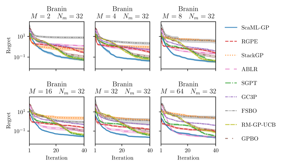
Figure 5: Experimental results on the Branin benchmark for different number of meta-tasks. Each meta-task is endowed with 32 points sampled uniformly at random from the task function’s domain $D$.

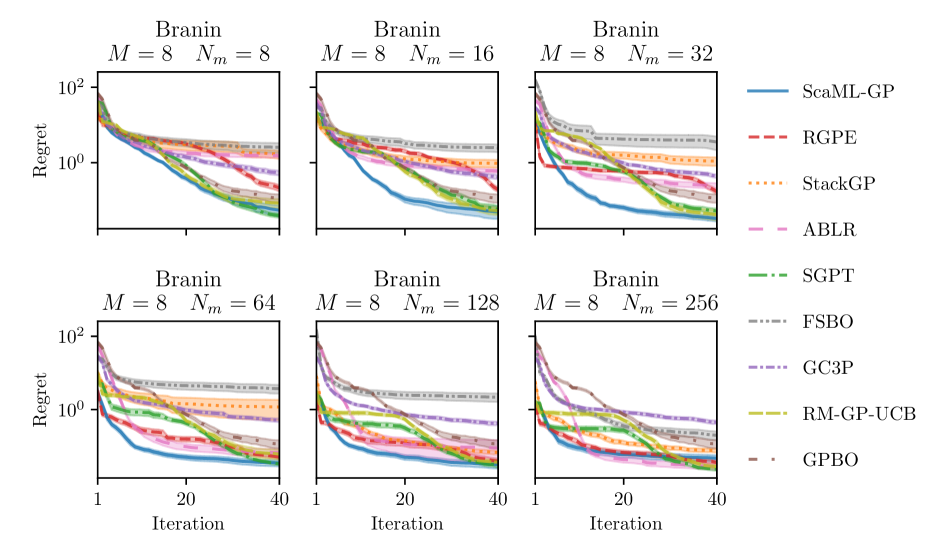
Figure 6: Experimental results on the Branin benchmark for different number of points per task, which are sampled uniformly at random from the task function’s domain $D$. Here, we keep the number of meta-tasks fixed to eight.

D.2 Ablation studies on the Hartmann6 benchmark

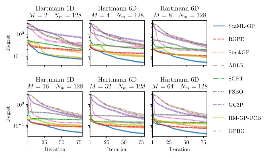
Figure 7: Experimental results on the Hartmann6 benchmark for different number of meta-tasks. Each meta-task is endowed with 128 points sampled uniformly at random from the task function’s domain $D$.

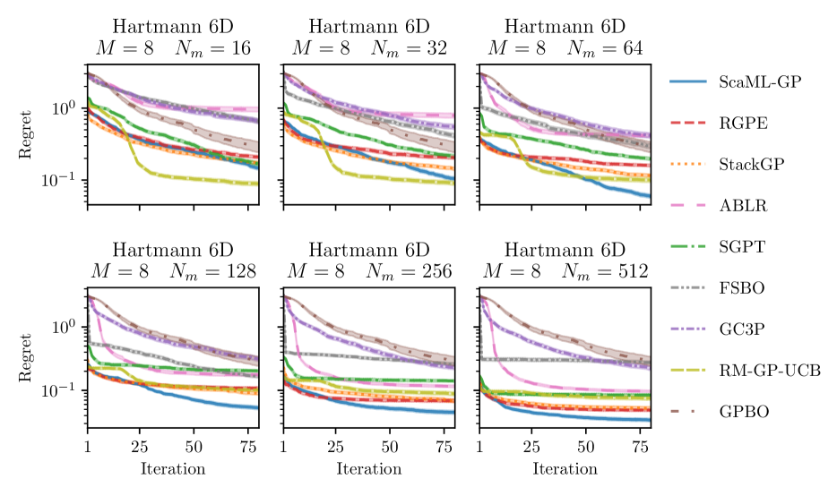
Figure 8: Experimental results on the Hartmann6 benchmark for different number of points per task, which are sampled uniformly at random from the task function’s domain $D$. Here, we keep the number of meta-tasks fixed to eight.

References

- Andrychowicz et al. (2016) Marcin Andrychowicz, Misha Denil, Sergio Gómez Colmenarejo, Matthew W. Hoffman, David Pfau, Tom Schaul, Brendan Shillingford, and Nando de Freitas. Learning to learn by gradient descent by gradient descent. In Proceedings of the 30th International Conference on Neural Information Processing Systems, page 3988–3996, Red Hook, NY, USA, 2016. Curran Associates Inc.
- Balandat et al. (2020) Maximilian Balandat, Brian Karrer, Daniel R. Jiang, Samuel Daulton, Benjamin Letham, Andrew Gordon Wilson, and Eytan Bakshy. BoTorch: A Framework for Efficient Monte-Carlo Bayesian Optimization. In Advances in Neural Information Processing Systems 33, 2020. URL http://arxiv.org/abs/1910.06403.
- Bayarri et al. (2009) M. J. Bayarri, J. O. Berger, and F. Liu. Modularization in Bayesian analysis, with emphasis on analysis of computer models. Bayesian Analysis, 4(1):119 – 150, 2009. doi: 10.1214/09-BA404.
- Bengio et al. (1991) Yoshua Bengio, Samy Bengio, and Jocelyn Cloutier. Learning a synaptic learning rule. In Proceedings of the International Joint Conference on Neural Networks, pages II–A969, Seattle, USA, 1991.
- Bonilla et al. (2008) Edwin V Bonilla, Kian Chai, and Christopher Williams. Multi-task gaussian process prediction. In J. Platt, D. Koller, Y. Singer, and S. Roweis, editors, Advances in Neural Information Processing Systems, volume 20. Curran Associates, Inc., 2008.
- Calandra et al. (2016) Roberto Calandra, André Seyfarth, Jan Peters, and Marc Peter Deisenroth. Bayesian optimization for learning gaits under uncertainty. Annals of Mathematics and Artificial Intelligence, 76(1):5–23, 2016.
- Chen et al. (2017) Yutian Chen, Matthew W. Hoffman, Sergio Gómez Colmenarejo, Misha Denil, Timothy P. Lillicrap, Matt Botvinick, and Nando de Freitas. Learning to learn without gradient descent by gradient descent. In Doina Precup and Yee Whye Teh, editors, Proceedings of the 34th International Conference on Machine Learning, volume 70 of Proceedings of Machine Learning Research, pages 748–756. PMLR, 06–11 Aug 2017.
- Dai et al. (2022) Zhongxiang Dai, Yizhou Chen, Haibin Yu, Bryan Kian Hsiang Low, and Patrick Jaillet. On provably robust meta-bayesian optimization. In Uncertainty in Artificial Intelligence, pages 475–485. PMLR, 2022.
- Duvenaud et al. (2011) David K Duvenaud, Hannes Nickisch, and Carl Rasmussen. Additive Gaussian Processes. Advances in Neural Information Processing Systems, 24, 2011.
- Eggensperger et al. (2021) Katharina Eggensperger, Philipp Müller, Neeratyoy Mallik, Matthias Feurer, Rene Sass, Aaron Klein, Noor Awad, Marius Lindauer, and Frank Hutter. HPOBench: A collection of reproducible multi-fidelity benchmark problems for HPO. In Thirty-fifth Conference on Neural Information Processing Systems Datasets and Benchmarks Track (Round 2), 2021. URL https://openreview.net/forum?id=1k4rJYEwda-.
- Feurer et al. (2018) Matthias Feurer, Benjamin Letham, and Eytan Bakshy. Scalable meta-learning for Bayesian optimization using ranking-weighted Gaussian process ensembles. In AutoML Workshop at ICML, volume 7, 2018.
- Finn et al. (2017) Chelsea Finn, Pieter Abbeel, and Sergey Levine. Model-agnostic meta-learning for fast adaptation of deep networks. In Doina Precup and Yee Whye Teh, editors, Proceedings of the 34th International Conference on Machine Learning, volume 70 of Proceedings of Machine Learning Research, pages 1126–1135. PMLR, 06–11 Aug 2017.
- Flennerhag et al. (2019) Sebastian Flennerhag, Pablo Garcia Moreno, Neil Lawrence, and Andreas Damianou. Transferring knowledge across learning processes. In International Conference on Learning Representations, 2019.
- Golovin et al. (2017) Daniel Golovin, Benjamin Solnik, Subhodeep Moitra, Greg Kochanski, John Karro, and D Sculley. Google vizier: A service for black-box optimization. In Proceedings of the 23rd ACM SIGKDD international conference on knowledge discovery and data mining, pages 1487–1495, 2017.
- Hariharan and Girshick (2017) Bharath Hariharan and Ross Girshick. Low-shot visual recognition by shrinking and hallucinating features. In Proceedings of the IEEE international conference on computer vision, pages 3018–3027, 2017.
- Jones et al. (1998) Donald R Jones, Matthias Schonlau, and William J Welch. Efficient global optimization of expensive black-box functions. Journal of Global optimization, 13(4):455–492, 1998.
- Joy et al. (2016) Tinu Theckel Joy, Santu Rana, Sunil Kumar Gupta, and Svetha Venkatesh. Flexible Transfer Learning Framework for Bayesian Optimisation. In James Bailey, Latifur Khan, Takashi Washio, Gill Dobbie, Joshua Zhexue Huang, and Ruili Wang, editors, Advances in Knowledge Discovery and Data Mining. Springer International Publishing, 2016.
- Lázaro-Gredilla et al. (2010) Miguel Lázaro-Gredilla, Joaquin Quinonero-Candela, Carl Edward Rasmussen, and Aníbal R Figueiras-Vidal. Sparse spectrum Gaussian process regression. The Journal of Machine Learning Research, 11:1865–1881, 2010.
- Li and Malik (2017) Ke Li and Jitendra Malik. Learning to optimize. In International Conference on Learning Representations, 2017. URL https://openreview.net/forum?id=ry4Vrt5gl.
- Liu et al. (2020) Haitao Liu, Yew-Soon Ong, Xiaobo Shen, and Jianfei Cai. When Gaussian Process Meets Big Data: A Review of Scalable GPs. IEEE Transactions on Neural Networks and Learning Systems, 31(11):4405–4423, 2020.
- Mallik (2021a) Neeratyoy Mallik. LogisticRegression. 8 2021a. doi: 10.6084/m9.figshare.15098283.v3. URL https://figshare.com/articles/dataset/LogisticRegression/15098283.
- Mallik (2021b) Neeratyoy Mallik. RandomForest. 8 2021b. doi: 10.6084/m9.figshare.15173517.v3. URL https://figshare.com/articles/dataset/RandomForest/15173517.
- Mallik (2021c) Neeratyoy Mallik. SupportVectorMachine. 8 2021c. doi: 10.6084/m9.figshare.15098280.v3. URL https://figshare.com/articles/dataset/SupportVectorMachine/15098280.
- Mallik (2021d) Neeratyoy Mallik. XGBoost. 8 2021d. doi: 10.6084/m9.figshare.15155919.v3. URL https://figshare.com/articles/dataset/XGBoost/15155919.
- Marco et al. (2017) Alonso Marco, Felix Berkenkamp, Philipp Hennig, Angela P. Schoellig, Andreas Krause, Stefan Schaal, and Sebastian Trimpe. Virtual vs. Real: Trading Off Simulations and Physical Experiments in Reinforcement Learning with Bayesian Optimization. In Proc. of the International Conference on Robotics and Automation (ICRA), pages 1557–1563, 2017.
- Metz et al. (2019) Luke Metz, Niru Maheswaranathan, Brian Cheung, and Jascha Sohl-Dickstein. Learning unsupervised learning rules. In International Conference on Learning Representations, 2019.
- Paleyes et al. (2019) Andrei Paleyes, Mark Pullin, Maren Mahsereci, Neil Lawrence, and Javier González. Emulation of physical processes with emukit. In Second Workshop on Machine Learning and the Physical Sciences, NeurIPS, 2019.
- Perrone et al. (2018) Valerio Perrone, Rodolphe Jenatton, Matthias W Seeger, and Cedric Archambeau. Scalable hyperparameter transfer learning. In S. Bengio, H. Wallach, H. Larochelle, K. Grauman, N. Cesa-Bianchi, and R. Garnett, editors, Advances in Neural Information Processing Systems, volume 31. Curran Associates, Inc., 2018.
- Poloczek et al. (2017) Matthias Poloczek, Jialei Wang, and Peter Frazier. Multi-information source optimization. In I. Guyon, U. V. Luxburg, S. Bengio, H. Wallach, R. Fergus, S. Vishwanathan, and R. Garnett, editors, Advances in Neural Information Processing Systems, volume 30. Curran Associates, Inc., 2017.
- Rasmussen and Williams (2006) Carl E. Rasmussen and Christopher K. I. Williams. Gaussian Processes for Machine Learning. Adaptive Computation and Machine Learning. MIT Press, Cambridge, MA, USA, January 2006.
- Rothfuss et al. (2022) Jonas Rothfuss, Christopher Koenig, Alisa Rupenyan, and Andreas Krause. Meta-learning priors for safe bayesian optimization. In 6th Annual Conference on Robot Learning, 2022.
- Salinas et al. (2020) David Salinas, Huibin Shen, and Valerio Perrone. A quantile-based approach for hyperparameter transfer learning. In Hal Daumé III and Aarti Singh, editors, Proceedings of the 37th International Conference on Machine Learning, volume 119 of Proceedings of Machine Learning Research, pages 8438–8448. PMLR, 13–18 Jul 2020.
- Schmidhuber (1987) Jürgen Schmidhuber. Evolutionary principles in self-referential learning, or on learning how to learn: The meta-meta-… hook. Diplomarbeit, Technische Universität München, München, 1987.
- Shahriari et al. (2016) Bobak Shahriari, Kevin Swersky, Ziyu Wang, Ryan P. Adams, and Nando de Freitas. Taking the human out of the loop: A review of bayesian optimization. Proceedings of the IEEE, 104(1):148–175, 2016.
- Shilton et al. (2017) Alistair Shilton, Sunil Gupta, Santu Rana, and Svetha Venkatesh. Regret Bounds for Transfer Learning in Bayesian Optimisation. In Aarti Singh and Jerry Zhu, editors, Proceedings of the 20th International Conference on Artificial Intelligence and Statistics, volume 54 of Proceedings of Machine Learning Research, pages 307–315, Fort Lauderdale, FL, USA, 20–22 Apr 2017. PMLR.
- Snoek et al. (2012) Jasper Snoek, Hugo Larochelle, and Ryan P Adams. Practical Bayesian Optimization of Machine Learning Algorithms. In F. Pereira, C. J. C. Burges, L. Bottou, and K. Q. Weinberger, editors, Advances in Neural Information Processing Systems, volume 25. Curran Associates, Inc., 2012.
- Srinivas et al. (2010) Niranjan Srinivas, Andreas Krause, Sham Kakade, and Matthias Seeger. Gaussian Process Optimization in the Bandit Setting: No Regret and Experimental Design. In Proc. International Conference on Machine Learning (ICML), 2010.
- Swersky et al. (2013) Kevin Swersky, Jasper Snoek, and Ryan P Adams. Multi-Task Bayesian Optimization. In C. J. C. Burges, L. Bottou, M. Welling, Z. Ghahramani, and K. Q. Weinberger, editors, Advances in Neural Information Processing Systems, volume 26. Curran Associates, Inc., 2013.
- Tighineanu et al. (2022) Petru Tighineanu, Kathrin Skubch, Paul Baireuther, Attila Reiss, Felix Berkenkamp, and Julia Vinogradska. Transfer Learning with Gaussian Processes for Bayesian Optimization. In International Conference on Artificial Intelligence and Statistics, pages 6152–6181. PMLR, 2022.
- Volpp et al. (2020) Michael Volpp, Lukas P. Fröhlich, Kirsten Fischer, Andreas Doerr, Stefan Falkner, Frank Hutter, and Christian Daniel. Meta-Learning Acquisition Functions for Transfer Learning in Bayesian Optimization. In International Conference on Learning Representations, 2020.
- Wang et al. (2016) Jane X Wang, Zeb Kurth-Nelson, Dhruva Tirumala, Hubert Soyer, Joel Z Leibo, Remi Munos, Charles Blundell, Dharshan Kumaran, and Matt Botvinick. Learning to reinforcement learn. arXiv preprint arXiv:1611.05763, 2016.
- Wang et al. (2021) Zi Wang, George E Dahl, Kevin Swersky, Chansoo Lee, Zelda Mariet, Zachary Nado, Justin Gilmer, Jasper Snoek, and Zoubin Ghahramani. Pre-trained Gaussian processes for Bayesian optimization. arXiv preprint arXiv:2109.08215, 2021.
- Wistuba and Grabocka (2021) Martin Wistuba and Josif Grabocka. Few-shot bayesian optimization with deep kernel surrogates. In International Conference on Learning Representations, 2021. URL https://openreview.net/forum?id=bJxgv5C3sYc.
- Wistuba et al. (2018) Martin Wistuba, Nicolas Schilling, and Lars Schmidt-Thieme. Scalable Gaussian process-based transfer surrogates for hyperparameter optimization. Machine Learning, 107(1):43–78, 2018.
- Yogatama and Mann (2014) Dani Yogatama and Gideon Mann. Efficient Transfer Learning Method for Automatic Hyperparameter Tuning. In Samuel Kaski and Jukka Corander, editors, Proceedings of the Seventeenth International Conference on Artificial Intelligence and Statistics, volume 33 of Proceedings of Machine Learning Research, pages 1077–1085, Reykjavik, Iceland, 22–25 Apr 2014. PMLR.
- Zhang et al. (2020) Yichi Zhang, Daniel W Apley, and Wei Chen. Bayesian optimization for materials design with mixed quantitative and qualitative variables. Scientific reports, 10(1):1–13, 2020.
- Álvarez et al. (2012) Mauricio A. Álvarez, Lorenzo Rosasco, and Neil D. Lawrence. Kernels for vector-valued functions: A review. Foundations and Trends in Machine Learning, 4(3):195–266, 2012.