A transform pair for bounded convex planar domains

Abstract

A new transform pair which can be used to solve mixed boundary value problems for Laplace’s equation and the complex Helmholtz equation in bounded convex planar domains is presented. This work is an extension of Crowdy (2015, CMFT, 15, 655–687) where new transform techniques were developed for boundary value problems for Laplace’s equation in circular domains. The key ingredient of the method is the analysis of the so called global relation which provides a coupling of integral transforms of the given boundary data and of the unknown boundary values. Three problems which involve mixed boundary conditions are solved in detail, as well as numerically implemented, to illustrate how to apply the new approach.

Keywords: transform pair; harmonic function; mixed boundary value problem.

1 Introduction

The Unified Transform Method (UTM) - a method for analysing boundary value problems for linear and integrable nonlinear PDEs - was pioneered in the late ’90s by A.S. Fokas [9]. From the very beginning, the UTM has attracted a great deal of interest in the applied mathematics community. A multitude of versions of the original method have since been developed, each dealing with a specific family of equations.

For the Laplace, biharmonic, Helmholtz and modified Helmholtz equations in convex polygonal domains, the UTM provides integral representations of the solutions in the complex Fourier plane (Fokas & Kapaev [10], Crowdy & Fokas [5], Dimakos & Fokas [7], Spence & Fokas [17], Davis & Fornberg [6]). Specifically, for Laplace’s equation, Fokas & Kapaev [10] developed a transform method for solving boundary value problems in simply connected polygonal domains. Their original approach relied on a variety of tools (spectral analysis of a parameter-dependent ODE; Riemann–Hilbert techniques, etc.). It was later observed by Crowdy [4] that the method can be recast within a complex function-theoretic framework; this, in turn, lead to the development of a new transform method applicable to so-called circular domains (domains bounded by arcs of circles, with line segments being a special case). Colbrook [1] extended the unified transform method to curvilinear polygons and PDEs with variable coefficients. In addition, Colbrook et al. [3] presented a hybrid analytical-numerical technique for elliptic PDEs based on the UTM, providing a fast and efficient method to evaluate the solution in the interior domain.

The focus of the present study is the extension of the original approach of Fokas & Kapaev [10] for convex polygons, to arbitrary convex domains. The method is built upon Crowdy’s [4] construction and it develops a new transform method for any convex bounded domain; this includes domains that may be non-circular or non-polygonal, such as ellipses. This study was motivated by engineering applications, in particular heat exchangers (namely the shell-and-tube exchangers) which have elliptical cross section (Saunders [14]) and the need of mathematical tools and transform methods to analyse problems in such geometries.

In §2, we present the theoretical framework needed to formulate the new transform pair for analytic functions in bounded convex planar domains. The new transform pair is presented in §3. The next step involves implementing the new transform in a variety of mixed boundary value problems (§4–6). In §7, we present the formulation of a transform pair for the complex Helmholtz equation. Finally, we conclude and discuss further applications in §8.

2 Theoretical framework

2.1 Preliminaries

A trapezoid is defined here to be a quadrilateral with at least one pair of parallel sides (there exist various definitions [12]). It follows from this definition that a trapezoid is a convex domain, given that the sum of the interior angles of a trapezoid is equal to $2\pi$.

Lemma 1.

Let $\Omega\subset\mathbb{C}$ be a bounded convex domain. For any $z_{0}\in\Omega$, there exists a trapezoid $T=T(z_{0})$ with the following properties:

1. Point $z_{0}$ is contained in the interior of $T$.

2. Two (parallel) sides of $T$ are each parallel to a coordinate axis.

3. The vertices of $T$ lie on the boundary of $\Omega$.

4. The closure of $T$ is contained in the closure of $\Omega$.

Proof.

First, note that a trapezoid satisfying properties 1–4 is not uniquely determined. To construct one such trapezoid, we first find an open disk lying in $\Omega$ containing $z_{0}$. In this disk, we inscribe a rectangle that contains $z_{0}$ with sides parallel to the coordinate axes. Ignoring, say, the vertical sides, we extend the horizontal sides of the rectangle until their vertices reach the boundary of $\Omega$. There is now only one way to connect these new vertices with straight line segments as to form a trapezoid that satisfies properties 1–4. Finally, the convexity assumption on $\Omega$ ensures that the closure of $T$ lies in the closure of $\Omega$. ∎

Remark 1: Without loss of generality, we assume that a coordinate system has been fixed where the coordinate axis of property 2 in Lemma 1 is the $x$-axis.

Remark 2: The vertices of $T$ partition the boundary of $\Omega$ into four adjacent arcs, where each arc is subtended by precisely one side of $T$.

Lemma 2.

For any $z,\zeta\in\mathbb{C}$ such that $0<\operatorname*{arg}(z-\zeta)<\pi$, we have

$$\lim_{t\rightarrow+\infty}\mathrm{e}^{\mathrm{i}t(z-\zeta)}=0.$$ (2.1)

Here $\mathrm{i}$ is the imaginary unit. Hence

$$\frac{1}{\zeta-z}\ =\mathrm{i}\int\limits_{0}^{\infty}\mathrm{e}^{\mathrm{i}t(z-\zeta)}\mathrm{d}t.$$ (2.2)

Proof.

The proof is a computation. ∎

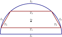
2.2 A labelling scheme

For domain $\Omega$ and trapezoid $T$ introduced in Lemma 1, we let $T_{k}$ and $v_{k}$, $k=1,\ldots,4$ denote the sides and vertices of $T$, respectively, where each label $k$ is assigned as follows. We label the lowest horizontal side $T_{1}$, and then label the remaining sides in ascending order as we travel along boundary of $T$ in the counterclockwise direction starting from $T_{1}$. For the vertices of $T$, we set $v_{1}$ to be the leftmost vertex of the side $T_{1}$ and then label the remaining vertices in ascending order as we travel along the boundary of $T$ in the counterclockwise direction. Finally, the four arcs that partition the boundary of $\Omega$ (see Remark 2) are denoted $I_{k}$, $k=1,\ldots,4$, where $I_{k}$ is subtended by $T_{k}$; see Figures 1(a)–1(b).

Remark 3: Since $\Omega$ is convex, we have that $I_{k}$ and the interior of $T$ lie on opposite sides of the line determined by $T_{k}$ for each $k=1,\ldots,4$.

((a)) A trapezoid $T$ (in red) inscribed in $\Omega$ (in blue), with labelling scheme.

((b)) A trapezoid $T$ (in red) inscribed in another $\Omega$ (in blue), with labelling scheme.

Figure 1: Example domains $T$ and $\Omega$.

Lemma 3.

Let $\Omega\subset\mathbb{C}$ be a given bounded convex domain; let $T$ be a trapezoid as in Lemma 1, and let $\{I_{1},\ldots,I_{4}\}$ be the corresponding partition of the boundary of $\Omega$. Then, for any $\alpha\in T$ and for any $k=1,\ldots,4$ there is $\beta_{k}\in[0,2\pi)$ such that the conformal affine map

$$\Psi_{k}(w)\coloneqq\mathrm{e}^{-\mathrm{i}\beta_{k}}(w-\alpha),\quad w\in\mathbb{C},$$ (2.3)

has

$$\operatorname*{Im}{(\Psi_{k}(\zeta))}<0,$$ (2.4)

and

$$\operatorname*{Im}(\Psi_{k}(\zeta))<\operatorname*{Im}(\Psi_{k}(z)),$$ (2.5)

for any $\zeta\in I_{k}$ and for any $z\in\textrm{int}(T)$.

Proof.

Since $\alpha$ is an interior point of $T$, it has positive distance from the boundary of $T$, including $T_{k}$, that is

$$0<\text{dist}(\alpha,T_{k})\coloneqq\inf\{|\alpha-z|:z\in T_{k}\}.$$ (2.6)

We now choose $\beta_{k}\in\mathbb{R}$ so that $\Psi_{k}$ in (2.3) has

$$\Psi_{k}(T_{k})\subset\{z:\operatorname*{Im}\,z=-\text{dist}(\alpha,T_{k})\}.$$ (2.7)

But the interior of $T$ and $I_{k}$ lie on opposite sides of $T_{k}$ (Remark 3.) and affine maps are rigid motions, thus $\Psi_{k}(int(T))$ and $\Psi_{k}(I_{k})$ must lie on opposite sides of $\Psi_{k}(T_{k})$ as well, and we choose $\beta_{k}\in[0,2\pi)$ so that

$$\Psi_{k}(I_{k})\subset\{w:\operatorname*{Im}\,w\leq-\text{dist}(\alpha,T_{k})\},$$ (2.8)

whereas

$$\Psi_{k}(int(T))\subset\{w:\operatorname*{Im}\,w>-\text{dist}(\alpha,T_{k})\}.$$ (2.9)

Now (2.4) follows from (2.6) and (2.8), while (2.6) and (2.9) give (2.5). ∎

Corollary 1.

With same notations and hypotheses as above, we have that

$$0<\operatorname*{arg}\big{(}\Psi_{k}(z)-\Psi_{k}(\zeta)\big{)}<\pi,$$ (2.10)

for any $z\in int(T)$ and any $\zeta\in I_{k}$.

This corollary is just a reformulation of $\eqref{E:in2}$ in such a way that it highlights the geometric condition needed to apply Lemma 2.

3 A new transform pair

With same notations as before, we may now give the following definitions. Let $\Omega$ be a simply connected and bounded domain. Let $C_{1},C_{2},\dots$ be a sequence of rectifiable Jordan curves that converges to $\partial\Omega$ in the sense that each compact subdomain of $\Omega$ is eventually contained in $C_{n}$ for large enough $n$. For $0<p\leq\infty$, we say that a holomorphic function $f\in O(\Omega)$ is in the Hardy Space $E^{p}(\Omega)$ (also known as Smirnov Class), if there is a positive and finite constant $M=M(f)$ such that

$$\int_{C_{n}}|f(\zeta)|^{p}\mathrm{d}\sigma<M<\infty,$$ (3.1)

for all $n$ and where $\mathrm{d}\sigma$ is arclength. If we further assume that $\Omega$ is bounded by a rectifiable Jordan curve, then we have that $f$ has a nontangential limit on $\partial\Omega$ $d\sigma$ almost everywhere which we also denote by $f$ and

$$\int_{\partial\Omega}|f|^{p}\mathrm{d}\sigma(\zeta)<\infty.$$ (3.2)

Note that $E^{p}(\Omega)$ will contain $O(\Omega)\cap C(\overline{\Omega})$. We have the following classical result found on page 170 of Duren’s Theory of $H^{p}$ Spaces [8].

Theorem 1.

If $f\in E^{1}(\Omega)$, then

$$f(z)=\frac{1}{2\pi i}\int_{\partial\Omega}\frac{f(\zeta)}{\zeta-z}\mathrm{d}\zeta,\qquad z\in\Omega,$$ (3.3)

and the integral vanishes for all $z$ outside of $\partial\Omega$.

Conversely, if $g\in L^{1}(\partial\Omega)$ and

$$\int_{\partial\Omega}\zeta^{n}g(\zeta)\mathrm{d}\zeta=0,\qquad n=0,1,2,\dots,$$ (3.4)

then

$$f(z)=\frac{1}{2\pi\mathrm{i}}\int_{\partial\Omega}\frac{g(\zeta)}{\zeta-z}\mathrm{d}\zeta\in E^{1}(\Omega),$$ (3.5)

and $g$ coincides $\mathrm{d}\sigma$ almost everywhere on $\partial\Omega$ with the nontangential limit of $f$.

Recall that $\mathrm{d}\sigma=d|\zeta|$ denotes arclength. In particular the theorem above implies that if $f\in E^{1}(\Omega)$ then $\int_{\partial\Omega}f(\zeta)\mathrm{d}\zeta=0$. Note that a detailed discussion on Hardy spaces over general domains is given in [8]. In the subsequent work, we will be interested in the Hardy space on bounded and convex domains. Convexity of a compact set in $\mathbb{R}^{n}$ implies the boundary is rectifiable. Thus we need not mention that the boundary of $\Omega$ must be rectifiable.

Definition 1.

Let $\Omega\subset\mathbb{C}$ be a bounded convex domain bounded by a Jordan curve and let $f\in E^{1}(\Omega)$. The spectral matrix $\{\rho_{jk}(t):t\in\mathbb{C}\}_{jk}$ has components

$${\rho_{jk}(t)=\int\limits_{I_{k}}f(\zeta)\mathrm{e}^{-\mathrm{i}t\mathrm{e}^{{-\mathrm{i}\beta_{j}}}\zeta}\mathrm{d}\zeta},\quad t\in\mathbb{C},\quad j,k=1,\ldots,4,$$ (3.6)

with $I_{k}$ and $\beta_{j}$ defined in §2. We shall refer to functions $\rho_{jk}(t)$ as spectral functions.

Lemma 4.

Using the same notation and assumptions as in Definition 1 above, the spectral functions $\rho_{jk}(t)$ are entire function for all $j,k=1,\ldots,4$, and

$$\sum_{k=1}^{4}\rho_{jk}(t)=0,\quad t\in\mathbb{C},\quad j=1,\ldots,4.$$ (3.7)

We refer to (7.16) as the global relations.

Theorem 2.

Let $\Omega\subset\mathbb{C}$ be a bounded convex domain bounded by a Jordan curve, let $T$ be a trapezoid as in Lemma 1, and let $f\in E^{1}(\Omega)$. Then, using the same notations as above, we have that

$$f(z)=\frac{1}{2\pi}\sum_{j=1}^{4}\int\limits_{0}^{\infty}\rho_{jj}(t)\,\mathrm{e}^{-\mathrm{i}\beta_{j}}\mathrm{e}^{\mathrm{i}t\mathrm{e}^{-\mathrm{i}\beta_{j}}z}\mathrm{d}t,\qquad\text{for any }z\in int(T).$$ (3.8)

We refer to (7.15) and (3.8) as the transform pair for bounded convex domains.

Proof.

Fix $\alpha\in T$ and recall the conformal affine maps obtained in Lemma 3:

$$\mathrm{e}^{-\mathrm{i}\beta_{j}}(w-\alpha)=\Psi_{j}(w),\quad 1\leq j\leq 4\,,\quad w\in\mathbb{C}.$$ (3.9)

Hence

$$\mathrm{e}^{-\mathrm{i}\beta_{j}}(z-\zeta)=\Psi_{j}(z)-\Psi_{j}(\zeta),\quad\text{for any}\ z,\zeta\in\mathbb{C}.$$ (3.10)

It follows from (3.10) and the definition of $\rho_{jj}(t)$ that

$$\mathrm{e}^{-\mathrm{i}\beta_{j}}\mathrm{e}^{\mathrm{i}t\mathrm{e}^{-\mathrm{i}\beta_{j}}z}\rho_{jj}(t)=\int\limits_{I_{j}}\!\!f(\zeta)\,\mathrm{e}^{-\mathrm{i}\beta_{j}}\mathrm{e}^{\mathrm{i}t(\Psi_{j}(z)-\Psi_{j}(\zeta))}\mathrm{d}\zeta.$$ (3.11)

This can be written as

$$\mathrm{e}^{-\mathrm{i}\beta_{j}}\mathrm{e}^{\mathrm{i}t\mathrm{e}^{-\mathrm{i}\beta_{j}}z}\rho_{jj}(t)=\int\limits_{I_{j}}\!\!f(\zeta)\,h_{z,\zeta}(t)\,\mathrm{d}\zeta,$$ (3.12)

where

$$h_{z,\zeta}(t)\coloneqq\mathrm{e}^{-\mathrm{i}\beta_{j}}\mathrm{e}^{\displaystyle{\mathrm{i}t(\Psi_{j}(z)-\Psi_{j}(\zeta))}},\quad t\in\mathbb{R}^{+}.$$ (3.13)

We claim that, for each $(z,\zeta)$, the absolute value of the function $h_{z,\zeta}$ (as a function of $t$) has finite integral on $\mathbb{R}^{+}$; more precisely,

$$h_{z,\zeta}(t)\in L^{1}(\mathbb{R}^{+},\mathrm{d}t),\quad\text{for any}\ (z,\zeta)\in int(T)\times I_{j}.$$ (3.14)

To see this, note that

$$|h_{z,\zeta}(t)|=\mathrm{e}^{\displaystyle{-t\,\operatorname*{Im}(\Psi_{j}(z)-\Psi_{j}(\zeta))}},\quad t\in\mathbb{R}^{+}.$$ (3.15)

But (2.5) implies that

$$c_{j,\zeta}\coloneqq\operatorname*{Im}(\Psi_{j}(z)-\Psi_{j}(\zeta))>0.$$ (3.16)

Hence

$$\int\limits_{0}^{\infty}|h_{z,\zeta}(t)|\,\mathrm{d}t=\int\limits_{0}^{\infty}\mathrm{e}^{\displaystyle{-t\,c_{j,\zeta}}}\,\mathrm{d}t=\lim_{t\to\infty}\frac{1}{c_{j,\zeta}}\left[1-\mathrm{e}^{\displaystyle{-t\,c_{j,\zeta}}}\right]=\frac{1}{c_{j,\zeta}}<\infty,$$ (3.17)

thus proving the claim. Note that there exists some $\epsilon>0$ such that $c_{j,\zeta}>\epsilon$ for $\zeta\in I_{j}$ (this follows from (2.8) and (2.9)).

Next we observe that since $f\in E^{1}(\Omega)$ then in particular $f\in L^{1}(\partial\Omega,\mathrm{d}\sigma)$ and hence $f\in L^{1}(I_{j},\mathrm{d}\sigma)$, $j=1,\ldots,4$, where $\mathrm{d}\sigma=|\mathrm{d}\zeta|$ is the arclength measure for $\partial\Omega$.

Using Cauchy’s integral formula

$$f(z)=\frac{1}{2\pi\mathrm{i}}\int\limits_{\partial\Omega}\frac{f(\zeta)}{\zeta-z}\mathrm{d}\zeta=\frac{1}{2\pi\mathrm{i}}\sum_{j=1}^{4}\int\limits_{I_{j}}\frac{f(\zeta)}{\zeta-z}\mathrm{d}\zeta,\qquad\text{for any}\ z\in\Omega.$$ (3.18)

But

$$\frac{1}{\zeta-z}=\frac{\mathrm{e}^{-i\beta_{j}}}{\Psi_{j}(\zeta)-\Psi_{j}(z)},\quad\text{for any}\ z\neq\zeta,$$ (3.19)

so that

$$f(z)=\frac{1}{2\pi\mathrm{i}}\int\limits_{\partial\Omega}\frac{f(\zeta)}{\zeta-z}\,\mathrm{d}\zeta=\frac{1}{2\pi\mathrm{i}}\sum_{j=1}^{4}\int\limits_{I_{j}}\frac{f(\zeta)\mathrm{e}^{-\mathrm{i}\beta_{j}}}{\Psi_{j}(\zeta)-\Psi_{j}(z)}\mathrm{d}\zeta,\qquad\text{for any}\ z\in\Omega.$$ (3.20)

Now, by Corollary 1, we have that

$$0<\textrm{Arg}(\Psi_{j}(z)-\Psi_{j}(\zeta))<\pi\quad\text{whenever}\ \ (z,\zeta)\in\text{int}(T)\times I_{j}.$$ (3.21)

Hence we may apply Lemma 2 and invoke the definition of $h_{z,\zeta}(t)$ to conclude that

$$\frac{\mathrm{e}^{-\mathrm{i}\beta_{j}}}{\Psi_{j}(\zeta)-\Psi_{j}(z)}=\mathrm{i}\int\limits_{0}^{\infty}h_{z,\zeta}(t)\,\mathrm{d}t,$$ (3.22)

for any $(z,\zeta)\in int(T)\times I_{j}$. Combining all of the above, we obtain

$$f(z)=\frac{1}{2\pi}\sum_{j=1}^{4}\int\limits_{I_{j}}f(\zeta)\int\limits_{0}^{\infty}h_{z,\zeta}(t)\mathrm{d}t\mathrm{d}\zeta.$$ (3.23)

Again, note that there exists some $\epsilon>0$ such that $c_{j,\zeta}>\epsilon$ for $\zeta\in I_{j}$ (this follows from (2.8) and (2.9)). Thus the integrand in (3.23) is bounded above uniformly in $\zeta\in I_{j}$, hence we may apply Fubini’s theorem to exchange the order of integration and obtain

$$f(z)=\frac{1}{2\pi}\sum_{j=1}^{4}\int\limits_{0}^{\infty}\int\limits_{I_{j}}f(\zeta)h_{z,\zeta}(t)\mathrm{d}\zeta\mathrm{d}t,$$ (3.24)

but by the definition of $h_{z,\zeta}(t)$ (see (3.11) and (3.12)), the latter is precisely the righthand side of (3.8), completing the proof of the theorem. ∎

Remark 4. Given $z\in\Omega$ there are many different choices of trapezoids $T$ that will work, each giving rise to a transform pair. In fact, any convex polygon inscribed in $\Omega$ will give rise to a transform pair. Each convex polygon will result in a unique partition of the boundary of $\Omega$. All such partitions (one for each choice of convex polygon) will produce comparable outcomes.

4 Dual Fourier Series for the disc

We consider the following incomplete Dirichlet boundary value problem for analytic functions in the unit disc $\mathbb{D}\coloneqq\{z\in\mathbb{C}~{}|~{}|z|<1\}$ for a given $m\in\mathbb{N}$:

$$\begin{cases}\overline{\partial}f(z)=0,\qquad|z|<1,\\ \\ \operatorname*{Re}f(\mathrm{e}^{\mathrm{i}\theta})=\cos m\theta,\qquad\theta\in C_{1}\coloneqq(-\pi/2,\pi/2),\\ \\ \operatorname*{Im}f(\mathrm{e}^{\mathrm{i}\theta})=-\sin m\theta,\qquad\theta\in C_{2}\coloneqq(\pi/2,3\pi/2).\end{cases}$$ (4.1)

(We refer to this problem as “incomplete”, because we only provide just the real part or the imaginary part of the boundary data, on each piece of the boundary.) This problem is uniquely solvable; it was originally solved by Shepherd [16] via a sequence of ingenious manipulations of integral representations of the Fourier series and was revisited by Crowdy [4].

Here we proceed as follows to obtain the solution. In the first step, we use one of the global relations (7.16) to extend the given (incomplete) boundary data to a function $f(\zeta)$ defined on the full boundary $\partial\mathbb{D}$. In the second step, we use our transform pair to numerically compute at a given point $z\in\mathbb{D}$ the (unique) solution of the completion of (4.1) to a Dirichlet problem on $\partial\mathbb{D}$.

We point out that the Dirichet problem above will have a unique solution in $E^{\infty}(\mathbb{D})$. Such a solution cannot be expressed in closed form, but can be computed numerically by the two steps mentioned previously. Note that the boundary data above may have many other solutions that to not belong to $E^{p}(\mathbb{D})$ for any $p\geq 1$. For instance, it is immediate to see that

$$f(\mathrm{e}^{\mathrm{i}\theta})\coloneqq\mathrm{e}^{-\mathrm{i}\,m\theta},\quad\theta\in(-\pi/2,3\pi/2],$$ (4.2)

is an extension of the given data to the full boundary, in fact:

$$f(\zeta)=\overline{\zeta}^{\,m},\quad\zeta\in\partial\mathbb{D}.$$ (4.3)

However this choice of $f(\zeta)$ has the unique harmonic extension

$$f(z)\coloneqq\overline{z}^{\,m},\quad z\in\overline{\mathbb{D}},$$ (4.4)

which does not solve (4.1) because it is not holomorphic. The main thrust of the global relations (7.16) is that any of them drives the numerical construction of the unique extension to $\partial\mathbb{D}$ belonging to $E^{\infty}(\mathbb{D})$ that solves (4.1).

The trapezoid in the transform pair derived above may be taken to be a rectangle with sides parallel to the coordinate axis. Thus for any $z\in\mathbb{D}$, we may find a rectangle $R$ as described in the previous sentence with $z\in R$ and use the following rectangle-like transform pair:

$$\begin{cases}\displaystyle{f(z)=\frac{1}{2\pi}\sum\limits_{n=1}^{4}\int\limits_{\mathcal{L}}c_{n}\mathrm{e}^{\mathrm{i}c_{n}tz}\rho_{nn}(t)\mathrm{d}t},\quad|z|<1,\\ \\ \displaystyle{\rho_{jn}(t)=\int\limits_{I_{n}(z)}\!\!\!f(\zeta)\mathrm{e}^{-\mathrm{i}c_{j}t\zeta}\mathrm{d}\zeta,\quad n,j=1,\ldots,4},\end{cases}$$ (4.5)

where

• $c_{j}\coloneqq\mathrm{e}^{\mathrm{i}\beta_{j}}$, $j=1,\ldots 4$ where $\beta_{j}=\pi(j-1)/2$, $n=1,2,3,4$.

• $\mathcal{L}$ is the fundamental contour. $\mathcal{L}\coloneqq(0,+\infty)$ (hence $t\in\mathbb{R}^{+}$)

• $\{I_{n}(z),\ n=1,\ldots,4\}$ is a partition of the unit circle into four disjoint “coordinate arcs” (each subtended by two points that determine a horizontal or vertical straight line segment) determined by the evaluation point $z$ in $\mathbb{D}$.

On $C_{1}$, we write, as in [4],

$$f(\mathrm{e}^{\mathrm{i}\theta})=\cos m\theta+\mathrm{i}\Big{(}a_{0}+\sum_{n\geq 1}\Big{[}a_{n}\mathrm{e}^{2\mathrm{i}n\theta}+\overline{a_{n}}\mathrm{e}^{-2\mathrm{i}n\theta}\Big{]}\Big{)},\quad\theta\in(-\pi/2,\pi/2),$$ (4.6)

where the coefficients $a_{0}\in\mathbb{R}$ and $\{a_{n}\in\mathbb{C}|n=1,2,\dots\}$ are to be determined. Similarly, on $C_{2}$, we write

$$f(\mathrm{e}^{i\theta})=b_{0}+\sum_{n\geq 1}\Big{[}b_{n}\mathrm{e}^{2\mathrm{i}n\theta}+\overline{b_{n}}\mathrm{e}^{-2\mathrm{i}n\theta}\Big{]}-\mathrm{i}\sin m\theta\,,\quad\theta\in(\pi/2,3\pi/2),$$ (4.7)

where coefficients $b_{0}\in\mathbb{R}$ and $\{b_{n}\in\mathbb{C}|n=1,2,\dots\}$ are to be determined. Recall the global relation given in (7.16):

$$\sum_{n=1}^{4}\rho_{1n}(t)=\sum_{n=1}^{4}\,\int\limits_{I_{n}(z)}\!\!\!f(\zeta)\mathrm{e}^{-\mathrm{i}t\zeta}\mathrm{d}\zeta=\int\limits_{\partial\mathbb{D}}f(\zeta)\mathrm{e}^{-\mathrm{i}t\zeta}\mathrm{d}\zeta=0,\quad t\in\mathbb{C}.$$ (4.8)

On substitution of (4.6) and (4.7) into (4.8), we obtain a linear system for the unknown coefficients given by

$$\begin{split}&a_{0}\mathcal{A}(0,t)+\sum_{n\geq 1}\Big{(}a_{n}\mathcal{A}(2n,t)+\overline{a_{n}}\mathcal{A}(-2n,t)\Big{)}\\ &~{}~{}~{}~{}~{}~{}+b_{0}\mathcal{B}(0,t)+\sum_{n\geq 1}\Big{(}b_{n}\mathcal{B}(2n,t)+\overline{b_{n}}\mathcal{B}(-2n,t)\Big{)}=r(t),\quad t\in\mathbb{C},\\ &a_{0}\overline{\mathcal{A}(0,t)}+\sum_{n\geq 1}\Big{(}\overline{a_{n}}\overline{\mathcal{A}(2n,t)}+a_{n}\overline{\mathcal{A}(-2n,t)}\Big{)}\\ &~{}~{}~{}~{}~{}~{}+b_{0}\overline{\mathcal{B}(0,t)}+\sum_{n\geq 1}\Big{(}\overline{b_{n}}\overline{\mathcal{B}(2n,t)}+b_{n}\overline{\mathcal{B}(-2n,t)}\Big{)}=\overline{r(t)},\quad t\in\mathbb{C},\end{split}$$ (4.9)

where

$$\begin{split}\mathcal{A}(n,t)&=-\int_{-\pi/2}^{\pi/2}\mathrm{e}^{-\mathrm{i}t\mathrm{e}^{\mathrm{i}\theta}}\mathrm{e}^{\mathrm{i}(n+1)\theta}\mathrm{d}\theta,\\ \mathcal{B}(n,t)&=\mathrm{i}\int_{\pi/2}^{3\pi/2}\mathrm{e}^{-\mathrm{i}t\mathrm{e}^{\mathrm{i}\theta}}\mathrm{e}^{\mathrm{i}(n+1)\theta}\mathrm{d}\theta,\end{split}$$ (4.10)

and the function $r(t)$ is defined by

$$r(t)=-\int_{\pi/2}^{3\pi/2}\sin(m\theta)\mathrm{e}^{-\mathrm{i}t\mathrm{e}^{\mathrm{i}\theta}}\mathrm{e}^{\mathrm{i}\theta}\mathrm{d}\theta-\mathrm{i}\int_{-\pi/2}^{\pi/2}\cos(m\theta)\mathrm{e}^{-\mathrm{i}t\mathrm{e}^{\mathrm{i}\theta}}\mathrm{e}^{\mathrm{i}\theta}\mathrm{d}\theta.$$ (4.11)

The equations above hold for all $t\in\mathbb{C}$. To proceed, the sums (4.6) and (4.7) (for $f(e^{i\theta})$) are truncated to include only terms up to $n=N$, and we formulate a linear system for the unknown coefficients $\{a_{n},b_{n}|n=0,\dots,N\}$. The linear system comprises of conditions (4.9) evaluated at points $t\in\mathbb{C}$ which are used to form an overdetermined linear system. This is then solved using least squares. Following an approach similar to Colbrook, et al. [2], points $t\in\mathbb{C}$ are chosen to be the origin and the concentric circles

$$\{t\in\mathbb{C}|t=-j/f^{\prime}(\mathrm{e}^{\mathrm{i}\theta}),\theta\in[0,2\pi],j=1,\dots,M_{r}\},$$ (4.12)

for some choice for the parameter $M_{r}$.

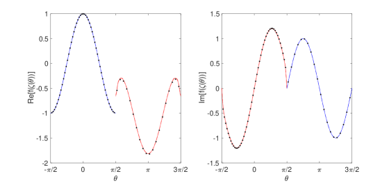
The solution of the linear system (4.9) shows that the coefficients $\{a_{n},b_{n}|n=0,\dots,N\}$ decay quickly and, therefore, we choose the truncation parameter to be $N=16$. Once the coefficients $\{a_{n},b_{n}|n=0,\dots,N\}$ are found, the spectral functions $\rho_{jk}(t)$ can be computed. The function$f(z)$ can be then computed via the transform pair (4.5). We have verified our numerical results with those obtained by Shepherd [16] and Crowdy [4]. Figure 2 shows the real and imaginary parts of $f(\zeta(\theta))$, $\theta\in[-\pi/2,3\pi/2]$ along the boundary of the unit disc computed using our new formulation, as well as Shepherd’s [16] and Crowdy’s [4] solutions. We observe that there appear to be discontinuities in the real part of $f$ for $\theta=\pi/2$ and $\theta=3\pi/2$ (also corresponding to $\theta=-\pi/2$), values at which the boundary conditions change type. Discontinuities as such are not surprising given the solution is in $E^{1}$.

Figure 2: Real (left) and imaginary (right) parts of $f(\zeta(\theta))$, $\theta\in[-\pi/2,3\pi/2]$ along the boundary of the unit disc, for $m=2$: new formulation for $N=16$ (solid lines), Crowdy’s [4] solution for the same truncation parameter (dashed lines) and Shepherd’s [16] solution (dots). The solutions via the new formulation and Crowdy’s [4] solution are indistinguishable.

5 Dual Fourier Series for the Ellipse

In this section, we present a generalization of the mixed boundary value problem considered by Shepherd [16] on the disc to a problem posed on an elliptical domain $D$, namely

$$D\coloneqq\left\{z\in\mathbb{C},x=\text{Re}[z],y=\text{Im}[z]\quad\Big{|}\quad\frac{x^{2}}{a^{2}}+\frac{y^{2}}{b^{2}}<1\right\},$$ (5.1)

whose boundary is

$$\partial D=\left\{z\in\mathbb{C},x=\text{Re}[z],y=\text{Im}[z]\quad\Big{|}\quad\frac{x^{2}}{a^{2}}+\frac{y^{2}}{b^{2}}=1\right\}.$$ (5.2)

We emphasize that the new methodology can be applied to solve boundary value problems in any convex domain; here we have chosen to focus on the ellipse. We consider the following incomplete boundary value problem for analytic functions

$$\begin{cases}\overline{\partial}f(z)=0,\qquad z\in D,\\ \\ \operatorname*{Re}f(\zeta)=\operatorname*{Re}\hskip 2.84526pt\overline{\zeta}^{m},\qquad\zeta\in\partial D\text{ and }\operatorname*{Re}\zeta>0,\\ \\ \operatorname*{Im}f(\zeta)=\operatorname*{Im}\hskip 2.84526pt\overline{\zeta}^{m},\qquad\zeta\in\partial D\text{ and }\operatorname*{Re}\zeta<0,\end{cases}$$ (5.3)

for a given $m\in\mathbb{N}$.

We parametrise the ellipse using polar coordinates $(\rho,\theta)$, with $0\leq\theta\leq 2\pi$ and

$$\rho(\theta)=\frac{ab}{\sqrt{(b\cos\theta)^{2}+(a\sin\theta)^{2}}}$$ (5.4)

and write

$$\zeta(\theta)\coloneqq\rho(\theta)\mathrm{e}^{\mathrm{i}\theta}\in D.$$ (5.5)

The boundary value problem (5.3) can be written in terms of polar coordinates as

$$\begin{cases}\overline{\partial}f(z)=0,\qquad z\in D,\\ \\ \operatorname*{Re}f=[\rho(\theta)]^{m}\cos m\theta,\qquad\theta\in C_{1}\coloneqq(-\pi/2,\pi/2),\\ \\ \operatorname*{Im}f=-[\rho(\theta)]^{m}\sin m\theta,\qquad\theta\in C_{2}\coloneqq(\pi/2,3\pi/2).\end{cases}$$ (5.6)

On $C_{1}$, we write

$$f(\theta,\rho(\theta))=[\rho(\theta)]^{m}\cos m\theta+\mathrm{i}\Big{(}a_{0}+\sum_{n\geq 1}\Big{[}a_{n}\mathrm{e}^{2\mathrm{i}n\theta}+\overline{a_{n}}\mathrm{e}^{-2\mathrm{i}n\theta}\Big{]}\Big{)}.$$ (5.7)

where coefficients $\{a_{n}\in\mathbb{C}|n=0,1,2,\dots\}$ are to be determined.

On $C_{2}$, we write

$$f(\theta,\rho(\theta))=\Big{(}b_{0}+\sum_{n\geq 1}\Big{[}b_{n}\mathrm{e}^{2\mathrm{i}n\theta}+\overline{b_{n}}\mathrm{e}^{-2\mathrm{i}n\theta}\Big{]}\Big{)}-\mathrm{i}[\rho(\theta)]^{m}\sin m\theta.$$ (5.8)

where coefficients $\{b_{n}\in\mathbb{C}|n=0,1,2,\dots\}$ are to be determined.

We have the following global relation:

$$\sum_{n=1}^{4}\rho_{1n}(t)=\sum_{n=1}^{4}\,\int\limits_{I_{n}(z)}\!\!\!f(\zeta)\mathrm{e}^{-\mathrm{i}t\zeta}\mathrm{d}\zeta=\int_{\partial D}f(\zeta)\mathrm{e}^{-\mathrm{i}t\zeta}\mathrm{d}\zeta=0,\quad t\in\mathbb{C},$$ (5.9)

where the last identity is due to Cauchy theorem applied to $F(\zeta)\coloneqq f(\zeta)\mathrm{e}^{-\mathrm{i}t\zeta}$ (which is analytic in $D$ for each fixed $t\in\mathbb{C}$. (Note that we need to strengthen our assumption on $f$ to ensure applicability of Cauchy theorem, e.g. $f\in H^{1}(D)$ as in the proceeding sections.)

On substitution of (5.7) and (5.8) into the global relation (5.9) and evaluation of (5.9) at certain values of $t\in\mathbb{C}$, we obtain a linear system for the unknown coefficients $\{a_{n},b_{n}|n=0,\dots,N\}$ of $f$. The linear system is given by (4.9), but now $\mathcal{A}(n,t)$, $\mathcal{B}(n,t)$ and $r(t)$ are defined by

$$\begin{split}\mathcal{A}(n,t)&=\mathrm{i}\int_{-\pi/2}^{\pi/2}\mathrm{e}^{-\mathrm{i}t\zeta(\theta)}\mathrm{e}^{\mathrm{i}n\theta}\zeta^{\prime}(\theta)\mathrm{d}\theta,\\ \mathcal{B}(n,t)&=\int_{\pi/2}^{3\pi/2}\mathrm{e}^{-\mathrm{i}t\zeta(\theta)}\mathrm{e}^{\mathrm{i}n\theta}\zeta^{\prime}(\theta)\mathrm{d}\theta,\end{split}$$ (5.10)

and

$$r(t)=-\int_{-\pi/2}^{\pi/2}[\rho(\theta)]^{m}\cos(m\theta)\mathrm{e}^{-\mathrm{i}t\zeta(\theta)}\zeta^{\prime}(\theta)\mathrm{d}\theta+\mathrm{i}\int_{\pi/2}^{3\pi/2}[\rho(\theta)]^{m}\sin(m\theta)\mathrm{e}^{-\mathrm{i}t\zeta(\theta)}\zeta^{\prime}(\theta)\mathrm{d}\theta.$$ (5.11)

Note that if $a=b=1$, i.e. we work with the unit circle, then expressions (5.10)–(5.11) become identical to (4.10)–(4.11).

The equations (4.9) hold for any $t\in\mathbb{C}$. To proceed, the sums (5.7) and (5.8) (for $f(\theta,\rho(\theta)$) are truncated to include only terms up to $n=N$ and we formulate a linear system for the unknown coefficients $\{a_{n},b_{n}|n=0,\dots,N\}$. The linear system comprises of conditions (4.9) evaluated at points $t\in\mathbb{C}$ which are used to form an overdetermined linear system.This is then solved using least squares. Following a similar approach to Colbrook et al. [2], points $t\in\mathbb{C}$ are chosen to be the origin and the concentric ellipses

$$\{t\in\mathbb{C}|t=-j/f^{\prime}(\theta,\rho(\theta)),\theta\in[0,2\pi],j=1,\dots,M_{r}\},$$ (5.12)

for some choice for the parameter $M_{r}$.

((a)) Parameters: $a=2$, $b=1$.

((b)) Parameters: $a=3$, $b=1$.

Figure 3: Real and imaginary parts of $f(\zeta(\theta))$, $\theta\in[-\pi/2,3\pi/2]$ along the boundary of the ellipse, for $m=2$.

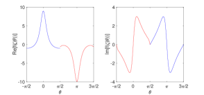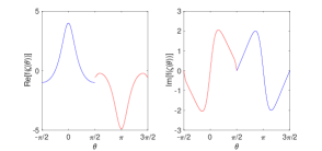
Similarly to the mixed boundary value problem posed on the unit disc presented in the previous section, we found that the coefficients $\{a_{n},b_{n}|n=0,\dots,N\}$ decay quickly and, therefore, we choose the truncation parameter to be $N=16$. Once the coefficients $\{a_{n},b_{n}|n=0,\dots,N\}$ are found, the spectral functions $\rho_{jk}(t)$ and $f(z)$ can be computed via the transform pair (4.5). Figure 3 shows the real and imaginary parts of $f(\zeta(\theta))$, $\theta\in[-\pi/2,3\pi/2]$ along the boundary of the ellipse, for $m=2$ and different parameter choices for $a$ and $b$. Similarly to the mixed boundary value problem on the unit disc presented in the previous section, we observe that there appear to be discontinuities in the real part of $f$ for $\theta=\pi/2$ and $\theta=3\pi/2$ (also corresponding to $\theta=-\pi/2$), values at which the boundary conditions change type. Discontinuities as such are not surprising given the solution is in $E^{1}$.

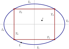
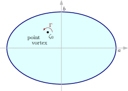
6 Application in fluid dynamics: A point vortex in the interior of an elliptical boundary

In this section, we present an application of the new formulation to a problem in fluid dynamics, in particular within the framework of a two-dimensional, inviscid, incompressible and irrotational (except of point vortices) steady flow. We consider a point vortex (namely, a vortex with infinite vorticity concentrated at a point) in the interior of a boundary with an elliptical shape and the aim is to find the resulting fluid flow satisfying the imposed impermeability boundary condition.

6.1 Problem formulation

We consider a point vortex at point $\zeta_{0}$ in the interior of the ellipse (5.1). A schematic of the configuration is shown in Figure 4. To begin, we introduce a complex potential function $h(z)$ and write

$$h(\zeta)=f_{s}(\zeta)+f(\zeta),$$ (6.1)

where

$$f_{s}(\zeta)=\frac{\Gamma}{2\pi\mathrm{i}}\log(\zeta-\zeta_{0}),$$ (6.2)

where $\Gamma\in\mathbb{R}$ is the circulation. The function $f(\zeta)$ is analytic in the ellipse and will be found using the transform method (3.8).

Figure 4: Schematic of the configuration: A point vortex at $\zeta_{0}$ in the interior of an elliptical boundary.

6.2 Solution scheme

6.2.1 Boundary condition

We impose an impermeability condition on the boundary of the ellipse:

$${\bf u}\cdot{\bf n}=0,$$ (6.3)

where ${\bf u}=(u,v)$ is the two-dimensional velocity field and ${\bf n}$ denotes the direction outward normal to the ellipse. Condition (6.3) can be expressed in terms of the complex potential as

$$\text{Im}[h(\zeta)]=0.$$ (6.4)

Substitution of (6.1) into (6.4) gives

$$\text{Im}[f(\zeta)]=-\text{Im}[f_{s}(\zeta)].$$ (6.5)

6.2.2 Function representation

We represent $f(\zeta)$ on the boundary of the ellipse using a Fourier expansion:

$$f(\zeta(\theta))=\Big{(}\sum_{n=0}^{\infty}a_{n}\mathrm{e}^{\mathrm{i}n\theta}+\sum_{n=0}^{\infty}\overline{a_{n}}\mathrm{e}^{-\mathrm{i}n\theta}\Big{)}-\mathrm{i}~{}\text{Im}[f_{s}(\zeta)],\quad\text{for }\theta\in[0,2\pi],$$ (6.6)

where coefficients $\{a_{n}\in\mathbb{C}|n=1,2,\dots\}$ are to be determined. The parametrization of the ellipse is given by

$$\zeta(\theta)=a\cos\theta+\mathrm{i}b\sin\theta,\quad\theta\in[0,2\pi].$$ (6.7)

Note that, since the imposed boundary condition (6.3) is the same along the entire elliptical boundary (in contrast to the previous problems where different conditions where imposed on different sections of the boundary), we have used a single representation (6.6) for $f(\zeta)$ to proceed instead of different representations on different sections of the boundary.

6.2.3 Spectral analysis

On substitution of (6.6) into the global relation (5.9), we obtain (after some algebra and rearrangement) a linear system for the unknown coefficients $\{a_{n}|n=1,\dots,N\}$. The infinite sums are truncated to include terms up to $n=N$. The linear system is given by

$$\sum_{n=0}^{N}\Big{(}a_{n}P(n,t)+\overline{a_{n}}P(-n,t)\Big{)}=R(t),\quad\text{for }t\in\mathbb{C},$$ (6.8)

where

$$P(n,t)=\int_{0}^{2\pi}{\mathrm{e}^{\mathrm{i}n\theta}\mathrm{e}^{-\mathrm{i}t\zeta(\theta)}\zeta^{\prime}(\theta)\mathrm{d}\theta}$$ (6.9)

and

$$R(t)=\mathrm{i}\int_{0}^{2\pi}{\text{Im}[f_{s}(\zeta(\theta))]\mathrm{e}^{-\mathrm{i}t\zeta(\theta)}\zeta^{\prime}(\theta)\mathrm{d}\theta}.$$ (6.10)

The linear system comprises of (6.8) and its conjugate evaluated at points $t\in\mathbb{C}$ which are used to form an overdetermined linear system. The choice of points $t\in\mathbb{C}$ is the same as in the previous section and given by (5.12). We found that the coefficients $\{a_{n}|n=1,\dots,N\}$ decay quickly and, therefore, we choose the truncation parameter to be $N=16$. Once the coefficients are found, the spectral functions and $f(z)$ can be computed via the transform pair (4.5).

Our results were checked against an exact solution found using conformal mapping techniques; introduce the conformal mapping $\Phi$ from the ellipse $D$ in the $\zeta$-plane to the unit disc $\mathbb{D}$ in the $w$-plane to be given by (Schwarz [15]):

$$\begin{split}w=\Phi(\zeta)&=\sqrt{k}~{}\text{sn}\left(\frac{2K}{\pi}\sin^{-1}(\zeta),m\right),\end{split}$$ (6.11)

where $\text{sn}(\cdot,\cdot)$ is the Jacobi sn function and definition of parameters $k,K$ and $m$ is given in [15, 18]. The complex potential function for a point vortex in the ellipse is given by

$$H(w)=\frac{\Gamma}{2\pi\mathrm{i}}\log\left(\frac{w-w_{0}}{w-1/\overline{w_{0}}}\right),\qquad\text{with}\quad w_{0}=\Phi(\zeta_{0}).$$ (6.12)

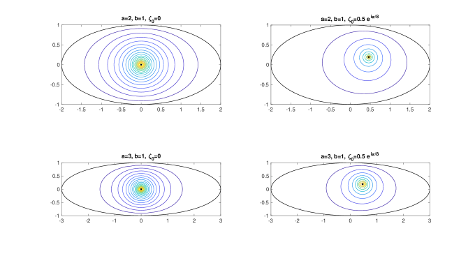
We have compared our results to (6.12) for interior points and the error at interior points was of the order $\mathcal{O}(10^{-4})$. To illustrate our results, Figure 5 shows the streamline pattern for a point vortex of strength $\Gamma=1$ at point $\zeta_{0}$ in the interior of an ellipse with parameters $a$ and $b$.

Figure 5: Streamlines for a point vortex of strength $\Gamma=1$ at point $\zeta_{0}$ in the interior of an ellipse with parameters $a$ and $b$.

7 The complex Helmholtz equation

In this section, we discuss how to obtain a transform pair for the complex Helmholtz equation in bounded convex planar domains.

Hauge & Crowdy [11] presented a transform method for the complex Helmholtz equation in polygonal domains using the theory of Bessels functions and Greens second identity. Given the geometric results of Lemma 3, here we develop a transform pair for the complex Helmholtz equation given by

$$\Delta\phi-4\sigma\phi=0,$$ (7.1)

where $\Delta=\nabla^{2}=\partial^{2}/\partial x^{2}+\partial^{2}/\partial y^{2}$ is the Laplacian operator and $0<\operatorname*{arg}(\sigma)<\pi$ that mirrors the transform pair for the $\overline{\partial}$ equation. Two results were pivotal in developing the transform pair for the $\overline{\partial}$ equation: the Cauchy integral formula and the desingularized Cauchy kernel. While a new integral representation for functions that satisfy the complex Helmholtz equation is required, Corollary 1 is still paramount in the desingularization of the new integral kernel.

7.1 An integral representation for solutions of the Helmholtz equation

The classical Green’s second identity:

$$\iint_{D}\Big{[}\phi\Delta\psi-\psi\Delta\phi\Big{]}\mathrm{d}A=\int_{\partial D}\phi\frac{\partial\psi}{\partial\mathbb{n}}-\psi\frac{\partial\psi}{\partial\mathbb{n}}\mathrm{d}s,$$ (7.2)

where $D$ is a bounded domain with piecewise $C^{2}$ boundary, $\mathrm{d}A$ is the Lebesgue measure and $\mathrm{d}s$ is the surface area measure, holds in $\mathbb{R}^{n}$ for twice continuously differentiable functions $\phi$ and $\psi$ that extend continuously to the boundary of $D$. If one restricts to $\mathbb{C}$ and uses the the identities

$$\frac{\partial^{2}}{\partial z\partial\overline{z}}=4\Delta,\qquad\mathrm{d}=\partial+\overline{\partial},\qquad\mathrm{d}A=\mathrm{d}x\mathrm{d}y=-2\mathrm{i}\mathrm{d}z\mathrm{d}\overline{z}$$ (7.3)

and Stokes’ theorem, we can write Green’s second identity in complex notation

$$\iint_{D}\Big{[}\phi\Delta\psi-\psi\Delta\phi\Big{]}\mathrm{d}A=2\mathrm{i}\int_{\partial D}\frac{\partial\phi}{\partial z}\psi\mathrm{d}z+\phi\frac{\partial\psi}{\partial\overline{z}}\mathrm{d}\overline{z}.$$ (7.4)

The (free space) Green’s Function $\mathcal{G}(z,z_{0})$ for the complex Helmholtz equation is defined as

$$\Delta\mathcal{G}(z,z_{0})-4\sigma\mathcal{G}(z,z_{0})=\delta(z-z_{0}).$$ (7.5)

If we let $G=\mathcal{G}$ and let $\phi$ be the solution to the complex Helmholtz equation (i.e. $\Delta\phi=4\sigma\phi$), then we get

$$\begin{split}\iint_{D}\Big{[}\phi(z)\Delta G(\zeta,z)-G(\zeta,z)\Delta\phi\Big{]}\mathrm{d}A&=\iint_{D}\Big{[}\phi(z)\Delta G(\zeta,z)-G(\zeta,z)4\sigma\phi(\zeta)\Big{]}\mathrm{d}A\\ &=\iint_{D}\phi(\zeta)\Big{[}\Delta G(\zeta,z)-G(\zeta,z)4\sigma\Big{]}\mathrm{d}A\\ &=\iint_{D}\phi(\zeta)\delta(\zeta-z)\mathrm{d}A\\ &=\phi(z).\end{split}$$ (7.6)

Hence we obtain

$$\phi(z)=2\mathrm{i}\int_{\partial D}\Big{[}\phi(\zeta)\frac{\partial G(\zeta,z)}{\partial\overline{\zeta}}\mathrm{d}\overline{\zeta}+G(\zeta,z)\frac{\partial\phi(\zeta)}{\partial\zeta}\mathrm{d}\zeta\Big{]}.$$ (7.7)

Note that the formula above gives us a way to recover interior values of $\phi$ by only knowing the boundary values of $\phi$. Formula (7.7) plays for the complex Helmholtz equation the analogous role as the Cauchy integral formula for the $\overline{\partial}$ equation. In order to compute this integral, one needs an explicit formula for $\mathcal{G}$.

7.2 The desingularization of the Green’s function

The Green’s function $\mathcal{G}$ for the complex Helmholtz equation can be expressed in terms of the order-zero modified Bessel function $K_{0}$. The function $K_{0}$ is axissymmetric, singular as $z\rightarrow z_{0}$ and decays as $z\rightarrow\infty$. For $\sigma$ as above, we have

$$\mathcal{G}(z,z_{0})=-\frac{1}{2\pi}K_{0}(2\sqrt{\sigma}|z-z_{0}|).$$ (7.8)

Hauge & Crowdy [11] gave an integral representation for $\mathcal{G}$.

$$K_{0}(z)=\frac{1}{2}\int_{L_{w}}\mathrm{e}^{-(z/2)(\alpha+1/\alpha)}\mathrm{d}\alpha/\alpha,\qquad-\frac{\pi}{2}<\arg(z)-\theta<\frac{\pi}{2},$$ (7.9)

where $\theta$ is the geometrical angle corresponding to the contour $L_{W}$ in the complex plane joining the two essential singularities of the integrand at 0 and $\infty$. The contour must be chosen so that the integrand decays along the contour as it approaches 0 and $\infty$. If we let $\theta_{0}$ be the angle that the contour makes with the at the origin, we need $-\pi/2<\arg(z)-\theta_{0}<\pi/2$. If the contour approaches $\infty$ at an angle of $\theta_{\infty}$, then we need $-\frac{\pi}{2}<\arg(z)+\theta_{\infty}<\frac{\pi}{2}$. If we choose $\theta_{0}=\theta_{\infty}$, and set $\theta=\theta_{0}$, the two inequalities above produce the same $\pi$-length range of possible arguments for $\arg u$. Letting $L_{\alpha}$ be a contour that approaches $0$ and $\infty$ at an angle of $\theta$, we have that

$$\mathcal{G}(z,z_{0})=-\frac{1}{4\pi}\int_{L_{\alpha}}\mathrm{e}^{-\sqrt{\sigma}|z-z_{0}|(\alpha+1/\alpha)}\frac{\mathrm{d}\alpha}{\alpha}.$$ (7.10)

Using the change of variables

$$-\mathrm{i}t\mathrm{e}^{\mathrm{i}\phi}=\sqrt{\sigma}\alpha,\qquad\phi=\arg(z-\zeta),$$ (7.11)

we define

$$G(\zeta,z)\coloneqq\mathcal{G}(\zeta,z)=-\frac{1}{4\pi}\int_{L^{(\sigma)}}\mathrm{e}^{\mathrm{i}t(z-\zeta)-\mathrm{i}\sigma\overline{(z-\zeta)}/t}\frac{\mathrm{d}t}{t},$$ (7.12)

where $L^{(\sigma)}$ is the contour $L_{\alpha}$ after the change of variables. Suppose now we pick a contour $L^{(\sigma)}_{0}$ so that our integral representation is valid for $0<\arg(z-\zeta)<\pi$. The exact contour does not matter, as long as we have $\theta_{0}=\arg(\sigma),\theta_{\infty}=0.$ So, we have

$$G(\zeta,z)=-\frac{1}{4\pi}\int_{L^{(\sigma)}_{0}}\mathrm{e}^{\mathrm{i}t(z-\zeta)-\mathrm{i}\sigma\overline{(z-\zeta)}/t}\frac{\mathrm{d}t}{t}.$$ (7.13)

Now suppose we wish to write the Green’s function for a different $\pi$-width range of arguments given by $\chi<\arg(z_{0}-z)<\chi+\pi$. Let $L^{(\sigma)}_{\chi}$ be such a contour so that integral representation of the Green’s function is valid for such $z$ and $z_{0}$. Again, the exact contour does not matter, as long as $\theta_{0}=\arg\sigma-\chi$, $\theta\infty=-\chi$. Then for this $\pi$-width range of arguments, we have

$$G(\zeta,z)=-\frac{1}{4\pi}\int_{L^{(\sigma)}_{\chi}}\mathrm{e}^{\mathrm{i}t(z-\zeta)-\mathrm{i}\sigma\overline{(z-\zeta)}/t}\frac{\mathrm{d}t}{t}.$$ (7.14)

Note that we may chose $L^{(\sigma)}_{\chi}$ to be the rotation through an angle of $-\chi$ of the contour $L^{(\sigma)}_{0}$.

7.3 Transform pair

Let $\Omega$ be a bounded convex domain in the complex plane. Let $z\in\Omega$. Lemma 1 gives a partition $\{I_{1},\dots,I_{4}\}$ of the boundary of $\Omega$. Using the notation established in section 2, we have the following definition.

Definition 2.

Let $\Omega$ be a bounded convex domain in $\mathbb{C}$ and let $\phi$ be a $C^{2}$ function in some neighborhood of $\Omega$ and a solution to the complex Helmholtz equation. The spectral functions $\{\rho_{j}(t):t\in\mathbb{C}\setminus\{0\}\}_{1\leq j\leq 4}$ are defined as

$$\rho_{j}(t)=\int_{I_{j}}\mathrm{e}^{-\mathrm{i}t\zeta+\mathrm{i}\sigma\overline{\zeta}/t}\Big{[}\phi(\zeta)(\mathrm{i}\sigma/t)\mathrm{d}\overline{\zeta}+\frac{\partial\phi(\zeta)}{\partial z}\mathrm{d}\zeta\Big{]},\qquad t\in\mathbb{C}\setminus\{0\},\quad j=1,\ldots,4.$$ (7.15)

Lemma 5.

With same notations and assumptions as above, we have

$$\sum_{j=1}^{4}\rho_{j}(t)=0\quad t\in\mathbb{C}\setminus\{0\},\quad j=1,\ldots,4.$$ (7.16)

We call (7.16) the global relation. Proof is presented in the Appendix A.1.

Theorem 3.

Let $\Omega$ be a bounded convex domain in $\mathbb{C}$ and let $\phi$ be a solution to the complex Helmholtz equation that is $C^{2}$ in some neighborhood of $\Omega$. Then, with same notations as above, we have that

$${\phi(z)=\frac{1}{2\pi\mathrm{i}}\sum_{j=1}^{4}\int_{L^{(\sigma)}_{\beta_{j}}}\mathrm{e}^{\mathrm{i}tz-\mathrm{i}\sigma\overline{z}/t}\rho_{j}(t)\frac{\mathrm{d}t}{t}}.$$ (7.17)

We refer to (7.15) and (7.17) as a transform pair. Proof is presented in the Appendix A.2.

8 Discussion

We have presented a new transform pair for Laplace’s equation and for the complex Helmholtz equation in bounded convex domains. Our work extends the work of Fokas & Kapaev [10] for convex polygons, to arbitrary convex domains. The method was built upon Crowdy’s [4] construction for Laplace’s equation in circular domains. We analysed mixed boundary value problems in circular and elliptical domains with different boundary conditions imposed on different sections of the boundary. Our results were verified against the solutions presented by Shepherd [16] and Crowdy [4] for the mixed boundary value problem on the unit disc.

The advantage of this study is that the new transform pairs and the approach presented in this paper can be algorithmically adapted to solve harmonic problems in bounded convex domains with mixed boundary conditions. We emphasise that, even though one can use conformal mapping techniques to analyse such problems, it becomes tricky or even impossible to find mappings for problems which involve mixed boundary conditions. We also note that this new approach can be also used to analyse boundary value problems for the biharmonic equation (which will involve solving for two analytic functions; Langlois [13]), as well as the complex Helmholtz equation as discussed in §7.

For future work, we aim to adapt the method for solving mixed boundary value problems in multiply connected domains. To solve such problems, one will need to construct transform pairs for non-convex domains, as well as to investigate the effect of having boundary components of different type (polygonal, circular or any smooth boundaries).

Funding

This work was partly supported by EPSRC grant no EP/R014604/1 and NSF-DMS-1901978 (Lanzani).

Appendix A Additions on the complex Helmholtz equation

A.1 Proof of Lemma 5

Proof.

First, set

$$\psi(\zeta)\coloneqq\mathrm{e}^{-\mathrm{i}t\zeta+\mathrm{i}\sigma\overline{\zeta}/t}.$$ (A.1)

A couple computations show

$$\Delta\psi=4\sigma\psi\quad\text{and}\quad\frac{\partial}{\partial\overline{\zeta}}\psi=\frac{\mathrm{i}\sigma}{t}\psi.$$ (A.2)

Indeed, setting $\zeta=x+\mathrm{i}y$, we have

$$\begin{split}\Delta\psi&=\frac{\partial^{2}}{\partial x^{2}}\mathrm{e}^{-\mathrm{i}t(x+\mathrm{i}y)+\mathrm{i}\sigma(x-\mathrm{i}y)/t}+\frac{\partial^{2}}{\partial y^{2}}\mathrm{e}^{-\mathrm{i}t(x+\mathrm{i}y)+\mathrm{i}\sigma(x-\mathrm{i}y)/t}\\ &=\frac{\partial}{\partial x}(-\mathrm{i}t+\mathrm{i}\sigma/t)\mathrm{e}^{-\mathrm{i}t(x+\mathrm{i}y)+\mathrm{i}\sigma(x-\mathrm{i}y)/t}+\frac{\partial}{\partial y}(t+\sigma/t)\mathrm{e}^{-\mathrm{i}t(x+\mathrm{i}y)+\mathrm{i}\sigma(x-\mathrm{i}y)/t}\\ &=(-\mathrm{i}t+\mathrm{i}\sigma/t)^{2}\mathrm{e}^{-\mathrm{i}t(x+\mathrm{i}y)+\mathrm{i}\sigma(x-\mathrm{i}y)/t}+(t+\sigma/t)^{2}\mathrm{e}^{-\mathrm{i}t(x+\mathrm{i}y)+\mathrm{i}\sigma(x-\mathrm{i}y)/t}\\ &=((-\mathrm{i}t+\mathrm{i}\sigma/t)^{2}+(t+\sigma/t)^{2})\psi\\ &=4\sigma\psi\end{split}$$ (A.3)

and

$$\frac{\partial}{\partial\overline{\zeta}}\psi=\frac{\partial}{\partial\overline{\zeta}}\mathrm{e}^{-\mathrm{i}t\zeta+\mathrm{i}\sigma\overline{\zeta}/t}=\big{[}\frac{\partial}{\partial\overline{\zeta}}(-\mathrm{i}t\zeta+\mathrm{i}\sigma\overline{\zeta}/t)\big{]}\mathrm{e}^{-\mathrm{i}t\zeta+\mathrm{i}\sigma\overline{\zeta}/t}=\frac{\mathrm{i}\sigma}{t}\psi.$$ (A.4)

Using these two computations above, the complex version of Green’s second identity, and $\Delta\phi=4\sigma\phi$ ($\phi$ is the solution to the Helmholtz equation), we have that

$$\begin{split}\sum_{j=1}^{4}\rho_{j}(t)&=\int_{\partial\Omega}\psi(\zeta)\Big{[}\phi(\zeta)(\mathrm{i}\sigma/t)\mathrm{d}\overline{\zeta}+\frac{\partial\phi(\zeta)}{\partial\zeta}\mathrm{d}\zeta\Big{]}\\ &=\int_{\partial\Omega}\Big{(}\frac{\partial}{\partial\overline{\zeta}}\psi(\zeta)\Big{)}\phi(\zeta)\mathrm{d}\overline{\zeta}+\frac{\partial\phi(\zeta)}{\partial\zeta}\psi(\zeta)\mathrm{d}\zeta\Big{]}\\ &=\frac{1}{2\mathrm{i}}\iint_{\Omega}\Big{(}\phi\Delta\psi-\psi\Delta\phi\Big{)}\mathrm{d}A\\ &=\frac{1}{2\mathrm{i}}\iint_{\Omega}\Big{(}\phi 4\sigma\psi-\psi 4\sigma\phi\Big{)}\mathrm{d}A=0.\end{split}$$ (A.5)

∎

A.2 Proof of Theorem 3

Proof.

Given a point $z\in\Omega$, we inscribe a trapezoid $T$ as in Lemma 1 that contains $z$. The vertices of $T$ partition the boundary of $T$ into 4 arcs, $I_{j}$, $1\leq j\leq 4$. For each $j$, we have the conformal affine map

$$\Psi_{j}(w)=\mathrm{e}^{-\mathrm{i}\beta_{j}}(w-\alpha).$$ (A.6)

Corollary 1 states that for $(z,\zeta)\in\text{int}(T)\times I_{j}$

$$0<\arg(\Psi_{j}(z)-\Psi_{j}(\zeta))<\pi.$$ (A.7)

A simple calculation shows

$$\mathrm{e}^{-\mathrm{i}\beta_{j}}(z-\zeta)=\Psi_{j}(z)-\Psi_{j}(\zeta),$$ (A.8)

so it follows that

$$\beta_{j}<\arg(z-\zeta)<\beta_{j}+\pi,$$ (A.9)

where $\beta_{j}\in[0,2\pi)$, $1\leq j\leq 4$ are angles of rotation determined by the trapezoid $T$ and $(z,\zeta)\in\text{int}(T)\times I_{j}$. We let $L^{(\sigma)}_{0}$ be a contour so that our integral representation for $G$ is valid for $0<\operatorname*{arg}(z-\zeta)<\pi$. For each $\beta_{j}$, $1\leq j\leq 4$, we may rotate $L^{(\sigma)}_{0}$ by $-\beta_{j}$ to get a contour $L^{(\sigma)}_{\beta_{j}}$ that is valid for $\beta_{j}<\arg(z-\zeta)<\beta_{j}+\pi$. Thus we get the following integral representation for $G$:

$$G(\zeta,z)=-\frac{1}{4\pi}\int_{L^{(\sigma)}_{\beta_{j}}}\mathrm{e}^{\mathrm{i}t(z-\zeta)-\mathrm{i}\sigma\overline{(z-\zeta)}/t}\frac{\mathrm{d}t}{t}$$ (A.10)

that is valid when

$$\beta_{j}<\arg(z-\zeta)<\beta_{j}+\pi,\qquad 0\leq\operatorname*{arg}(\sigma)<\pi.$$ (A.11)

If we let $\phi$ be the solution to the complex Helmholtz equation, then we have the following integral representation for $\phi$ that follows from Green’s second identity:

$$\phi(z)=2\mathrm{i}\int_{\partial\Omega}\Big{[}\phi(\zeta)\frac{\partial G(\zeta,z)}{\partial\overline{\zeta}}\mathrm{d}\overline{\zeta}+G(\zeta,z)\frac{\partial\phi(\zeta)}{\partial\zeta}\mathrm{d}\zeta\Big{]}.$$ (A.12)

A quick calculation shows that

$$\frac{\partial G(\zeta,z)}{\partial\overline{\zeta}}=-\frac{1}{4\pi}\int_{L^{(\sigma)}_{\beta_{j}}}\mathrm{e}^{\mathrm{i}t(z-\zeta)-\mathrm{i}\sigma\overline{(z-\zeta)}/t}\frac{\mathrm{i}\sigma}{t}\frac{\mathrm{d}t}{t}.$$ (A.13)

Now that we have a valid integral representation for $G$ and $\partial G/\partial\bar{\zeta}$ for each $I_{j}$, we can use Fubini’s theorem and see that

$$\begin{split}\phi(z)&=2\mathrm{i}\sum_{j=1}^{k}\int_{I_{j}}\Big{[}\phi(\zeta)\frac{\partial G(\zeta,z)}{\partial\overline{\zeta}}\mathrm{d}\overline{\zeta}+G(\zeta,z)\frac{\partial\phi(\zeta)}{\partial\zeta}d\zeta\Big{]}\\ &=\frac{1}{2\pi\mathrm{i}}\sum_{j=1}^{4}\int_{I_{j}}\int_{L_{\beta_{j}}^{(\sigma)}}\mathrm{e}^{\mathrm{i}t(z-\zeta)-\mathrm{i}\sigma\overline{(z-\zeta)}/t}\big{[}\phi(\zeta)(\mathrm{i}\sigma/t)\mathrm{d}\overline{\zeta}+\frac{\partial\phi(\zeta)}{\partial\zeta}\mathrm{d}\zeta\big{]}\frac{\mathrm{d}t}{t}\\ &=\frac{1}{2\pi\mathrm{i}}\sum_{j=1}^{4}\int_{L^{(\sigma)}_{\beta_{j}}}\mathrm{e}^{\mathrm{i}tz-\mathrm{i}\sigma\overline{z}/t}\rho_{j}(t)\frac{\mathrm{d}t}{t}.\end{split}$$ (A.14)

∎

References

- [1] M. J. Colbrook. Extending the unified transform: curvilinear polygons and variable coefficient PDEs. IMA J. Numer. Anal., 40(2):976–1004, 2020.
- [2] M. J. Colbrook, N. Flyer, and B. Fornberg. On the Fokas method for the solution of elliptic problems in both convex and non-convex polygonal domains. J. Comput. Phys., 374:996–1016, 2018.
- [3] M. J. Colbrook, A. S. Fokas, and P. Hashemzadeh. A hybrid analytical-numerical technique for elliptic PDEs. SIAM J. Sci. Comput., 41(2):1066–1090, 2019.
- [4] D. G. Crowdy. Fourier–Mellin transforms for circular domains. Comput. Methods Funct. Th., 15(4):655 – 687, 2015.
- [5] D. G. Crowdy and A. S. Fokas. Explicit integral solutions for the plane elastostatic semi-strip. Proc. R. Soc. Lond. A, 460:1285–1310, 2004.
- [6] C. Davis and B. Fornberg. A spectrally accurate numerical implementation of the Fokas transform method for Helmholtz-type PDEs. Complex. Var. Elliptic, 59:564–577, 2014.
- [7] M. Dimakos and A. S. Fokas. The Poisson and the biharmonic equations in the interior of a convex polygon. Stud. Appl. Math., 134:456–498, 2015.
- [8] P. L. Duren. Theory of spaces. Academic Press, 1970.
- [9] A. S. Fokas. A unified transform method for solving linear and certain nonlinear PDEs. Proc. Roy. Soc. London Ser. A, 453:1411–1443, 1997.
- [10] A. S. Fokas and A. A. Kapaev. On a transform method for the Laplace equation in a polygon. IMA J. Appl. Math., 68:355–408, 2003.
- [11] J. C. Hauge and D. G. Crowdy. A new approach to the complex Helmholtz equation with application to diffusion wave fields, impedance spectroscopy and unsteady Stokes flow. IMA J. Appl. Math., 86:1287–1326, 2021.
- [12] M. Joseffson. Characterizations of trapezoids. Forum Geometricorum, 13:23–35, 2013.
- [13] W. E. Langlois. Slow viscous flows. Macmillan, New York, NY, 1964.
- [14] E. A. D. Saunders. Heat exchangers : selection, design and construction. Longman Scientific & Technical ; John Wiley & Sons, 1988.
- [15] H.A. Schwarz. Über einige Abbildungsaufgaben. J. Reine Angew. Math., 70:105–120, 1869.
- [16] W. M. Shepherd. On trigonometric series with mixed conditions. Proc. Lond. Math. Soc., 2(43):366–375, 1937.
- [17] E. Spence and A. S. Fokas. A new transform method I: domain-dependent fundamental solutions and integral representations. Proc. R. Soc. A, 466:2259–2281, 2010.
- [18] G. Szegő. Conformal mapping of the interior of an ellipse onto a circle. The American Mathematical Monthly, 57(7):474–478, 1950.