Neural networks for the approximation of Euler’s elastica

Abstract

Euler’s elastica is a classical model of flexible slender structures, relevant in many industrial applications. Static equilibrium equations can be derived via a variational principle. The accurate approximation of solutions of this problem can be challenging due to nonlinearity and constraints. We here present two neural network based approaches for the simulation of this Euler’s elastica. Starting from a data set of solutions of the discretised static equilibria, we train the neural networks to produce solutions for unseen boundary conditions. We present a discrete approach learning discrete solutions from the discrete data. We then consider a continuous approach using the same training data set, but learning continuous solutions to the problem. We present numerical evidence that the proposed neural networks can effectively approximate configurations of the planar Euler’s elastica for a range of different boundary conditions.

1 Introduction

Modelling of mechanical systems is relevant in various branches of engineering. Typically, it leads to the formulation of variational problems and differential equations, whose solutions are approximated with numerical techniques. The efficient solution of linear and non-linear systems resulting from the discretisation of mechanical problems has been a persistent challenge of applied mathematics. While classical solvers are characterised by a well-established and mature body of literature [1, 2, 3, 4, 5, 6, 7], the past decade has witnessed a surge in the use of novel machine learning-assisted techniques [8, 9, 10, 11, 12, 13, 14, 15, 16, 17, 18, 19, 20, 21, 22, 23, 24]. These approaches aim at enhancing solution methods by leveraging the wealth of available data and known physical principles. The use of deep learning techniques to improve the performance of traditional numerical algorithms in terms of efficiency, accuracy, and computational scalability, is becoming increasingly popular also in computational mechanics. Examples comprise virtually any problem where approximation of functions is required, but also efficient reduced order modelling e.g. in fluid mechanics, the deep Ritz method, or more specific numerical tasks such as optimisation of the quadrature rule for the computation of the finite element stiffness matrix, acceleration of simulations on coarser meshes by learning appropriate collocation points, and replacing expensive numerical computations with data-driven predictions [9, 25, 26, 27, 12]. This recent literature is evidence that neural networks can be used successfully as surrogate models for the solution operators of various differential equations.

In the context of ordinary and partial differential equations, two main trends can be identified. The first one aims at providing a machine learning based approximation to the discrete solutions of differential problems on a certain space-time grid, for example by solving linear or nonlinear systems efficiently and accelerating convergence of iterative schemes [20, 19, 15, 14, 13]. The second one provides instead solutions to the differential problem as continuous (and differentiable) functions of the temporal and spatial variables. Depending on the context, conditions on such approximate solutions are then provided by the differential problem itself, by the initial values and the boundary conditions, and by the available data. The idea of providing approximate solutions as functions defined on the space-time domain and parametrised as neural networks was proposed in the nineties [28] and was recently revived in the framework of Physics-Informed Neural Networks in [10]. Since then, such an approach has attracted a lot of interest and has developed in many directions [8, 21, 25].

In this work, we use neural networks to approximate the configurations of highly flexible slender structures modelled as beams. Such models are of great interest in industrial applications like cable car ropes, diverse types of wires or endoscopes [29, 30, 31, 32]. Notwithstanding their ingenious and simple mathematical formulation, slender structure models can accurately reproduce complex mechanical behaviour and for this reason their numerical discretisation is often challenging. Furthermore, the use of 3-dimensional models requires high computational time. Due to the fact that slender deformable structures have one dimension (length) being orders of magnitude larger than their other dimensions (cross-section), it is possible to reduce the complexity of the problem from a $3$-dimensional elastic continuum to a $1$-dimensional beam. A beam is modelled as a centerline curve, $\mathbf{q}:[0,L]\to\mathbb{R}^{n},s\mapsto\mathbf{q}(s)$, with $n=2$ or $n=3$, along which a rigid cross-section $\Sigma(s)$ is attached. The main model assumption is that the diameter of $\Sigma(s)$ is small compared with the undeformed length $L$. We here consider a special case of a beam where the cross-section $\Sigma(s)$ is constant and orthogonal to the centerline, the $2$-dimensional Euler’s elastica [33]. In this case, $\mathbf{q}(s)$ is inextensible with fixed boundary conditions and is the solution of a bending energy minimisation problem [34, 35, 36].

When approximating static equilibria of the Euler’s elastica via neural networks, a key issue is to ensure the inextensibility of the curve (having unit norm tangents) as well as the boundary conditions. Two main approaches can be found in the literature [25, 21, 37]. One is the weak imposition of constraints and boundary conditions adding appropriate, extra terms to the loss function. The other is a strong imposition strategy consisting in shaping the network architectures so that they satisfy the constraints by construction. We show examples of both the approaches in Sections 4 and 5.

The paper is organised as follows. In Section 2, we present the mathematical model of the planar Euler’s elastica, including its continuous and discrete equilibrium equations. We describe the approach used to generate the data sets for the numerical experiments. In Section 3, we introduce some basic theory and notation for neural networks that we shall use in the succeeding sections. Starting from general theory, we specialise in the task of approximating configurations of the Euler’s elastica. In Section 4, we introduce the discrete approach, which aims to approximate precomputed numerical discretisations of the Euler’s elastica. We discuss some drawbacks associated with this approach and then propose an alternative approximation strategy in Section 5. The continuous approach consists in computing an arc length parametrisation of the beam configuration. We provide insights into two additional networks and analyse how the test accuracy changes with varying constraints, such as boundary conditions or tangent vector norms. Data and codes for the numerical experiments are available in the GitHub repository associated to the paper .

Main contributions: This paper presents advancements in the approximation of beam configurations using neural networks. These advancements include: (i) An extensive experimental analysis of approximating numerical discretisations of Euler’s elastica configurations through what we call discrete networks, (ii) Identification and discussion of the limitations associated with this discrete approach, and (iii) Introduction of a new parametrisation strategy called continuous network to address some of these drawbacks.

Nomenclature
$\mathcal{L}$	continuous Lagrangian function
$\mathcal{S}$	continuous action functional
$\mathcal{L}_{d}$	discrete Lagrangian function
$\mathcal{S}_{d}$	discrete action functional
$\mathbf{q}$	configuration of the beam
$\mathbf{q}^{\prime}$	first spatial derivative of $\mathbf{q}$
$\theta$	tangential angle
$s$	arc length parameter
$\kappa$	curvature
$L$	length of the undeformed beam
$EI$	bending stiffness, with $E$ the elastic modulus and $I$ the second moment of area
$\hat{\mathbf{q}}$	numerical approximation of $\mathbf{q}$
$N+1$	number of discretisation nodes, with $N$ the number of intervals
$h$	space step (length of each interval)
$q_{\boldsymbol{\rho}}^{\textrm{d}}$	discrete neural network
$q_{\boldsymbol{\rho}}^{\textrm{c}}$	continuous neural network approximating the solution curve $\boldsymbol{q}(s)$
$\theta_{\boldsymbol{\rho}}^{\textrm{c}}$	continuous neural network approximating the angular function $\theta(s)$
$\boldsymbol{\rho}$	parameters of the neural network
$\ell$	number of layers in the neural network
$\sigma$	activation function
$M$	number of training data
$B$	size of one training batch
MSE	mean squared error
MLP	multi layer perceptron
ResNet	residual neural network
MULT	multiplicative neural network
$\mathcal{D}$	differential operator
$\mathcal{I}$	quadrature operator

Table 1: List of abbreviations and notations.

2 Euler’s elastica model

We consider an inextensible beam model in which the cross-section $\Sigma(s)$ is assumed to be constant along the arc length $s$ and perpendicular to the centerline $\mathbf{q}(s)$, which means that no shear deformation can occur. Thus, the deformation of the centerline is a pure bending problem, precisely the Euler’s elastica curve. In the following, we assume $\mathbf{q}\in C^{2}([0,L],\mathbb{R}^{2})$, i.e., the curve is planar and twice continuously differentiable with length $L$. If $s$ denotes the arc length parameter, then $\|\mathbf{q}^{\prime}(s)\|=1$, where ${}^{\prime}=\frac{d}{ds}$, for all $s\in[0,L]$. The elastica problem consists in minimising the following Euler-Bernoulli energy functional

$$\int_{0}^{L}\kappa(s)^{2}ds,$$

where $\kappa(s)$ denotes the curvature of $\mathbf{q}(s)$, [35]. Given the arc length parametrisation, then $\kappa(s)=\|\mathbf{q}^{\prime\prime}(s)\|$.

We can reformulate this problem as a constrained Lagrangian problem as follows. Consider the second-order Lagrangian $\mathcal{L}:T^{(2)}Q\rightarrow\mathbb{R}$, where $T^{(2)}Q$ denotes the second-order tangent bundle [38] of the configuration manifold $Q$, which in this case is $\mathbb{R}^{2}$:

$$\mathcal{L}\left(\mathbf{q},\mathbf{q}^{\prime},\mathbf{q}^{\prime\prime}\right)=\frac{1}{2}EI\left\|\mathbf{q}^{\prime\prime}\right\|^{2}\,.$$ (1)

Here, abusing the notation, ^′ denotes a spatial derivative, but we do not initially assume arc length parametrisation. The parameter $EI$ is the bending stiffness, which governs the response of the elastica under bending. This mechanical parameter consists of a material and a geometric properties, where $E$ is the Young’s modulus and $I$ is the second moment of area of the cross-section $\Sigma$. For simplicity, these parameters are assumed to be constant along the length of the beam.

In order to recover the solutions of the elastica, the Lagrangian in Equation (1) must be supplemented with the constraint equation

$$\Phi(\mathbf{q},\mathbf{q}^{\prime})=\|\mathbf{q}^{\prime}\|^{2}-1=0.$$ (2)

This imposes arc length parametrisation of the curve $\mathbf{q}(s)$ and leads to the augmented Lagrangian $\widetilde{\mathcal{L}}:T^{(2)}Q\times\mathbb{R}\rightarrow\mathbb{R}$

$$\widetilde{\mathcal{L}}\left(\mathbf{q},\mathbf{q}^{\prime},\mathbf{q}^{\prime\prime},\Lambda\right)=\mathcal{L}\left(\mathbf{q},\mathbf{q}^{\prime},\mathbf{q}^{\prime\prime}\right)+\Lambda\Phi(\mathbf{q},\mathbf{q}^{\prime}),$$ (3)

where $\Lambda(s)$ is a Lagrange multiplier, see [36]. The Lagrangian function coincides with the total elastic energy over solutions of the corresponding Euler-Lagrange equations. The internal bending moment is directly related to the curvature $\kappa(s)$.

The continuous action functional $\mathcal{S}$ is defined as:

$$\mathcal{S}[\mathbf{q}]=\int_{0}^{L}\widetilde{\mathcal{L}}\left(\mathbf{q},\mathbf{q}^{\prime},\mathbf{q}^{\prime\prime},\Lambda\right)\,ds.$$ (4)

Applying Hamilton’s principle of stationary action, $\delta\mathcal{S}=0$, yields the Euler-Lagrange equations

$$\frac{d^{2}}{ds^{2}}\left(\frac{\partial\mathcal{L}}{\partial\mathbf{q}^{\prime\prime}}\right)-\frac{d}{ds}\left(\frac{\partial\mathcal{L}}{\partial\mathbf{q}^{\prime}}\right)+\frac{\partial\mathcal{L}}{\partial\mathbf{q}} =\frac{d}{ds}\left(\frac{\partial\Phi}{\partial\mathbf{q}^{\prime}}\Lambda\right)-\frac{\partial\Phi}{\partial\mathbf{q}}\Lambda,$$ (5)

$$\|\mathbf{q}^{\prime}\|^{2}-1 =0,$$

which need to be satisfied together with the boundary conditions on positions and tangents, i.e.,$(\mathbf{q}(0),\mathbf{q}^{\prime}(0))=(\mathbf{q}_{0},\mathbf{q}^{\prime}_{0})$ and $(\mathbf{q}(L),\mathbf{q}^{\prime}(L))=(\mathbf{q}_{N},\mathbf{q}^{\prime}_{N})$.

2.1 Space discretisation of the elastica

The continuous augmented Lagrangian $\widetilde{\mathcal{L}}$ in Equation (3) and the action integral $\mathcal{S}$ in Equation (4) are discretised over the beam length $L$ with constant space steps $h$ and $N+1$ equidistant nodes $0=s_{0}<s_{1}<\ldots<s_{N-1}<s_{N}=L$. In second-order systems, the discrete Lagrangian is a function $\widetilde{L}_{d}:TQ\times TQ\times\mathbb{R}\times\mathbb{R}\rightarrow\mathbb{R}$. In this study, we refer to a discretisation of the Lagrangian function proposed in [39] based on the trapezoidal rule:

$$\begin{split}&\widetilde{\mathcal{L}}_{d}\left(\mathbf{q}_{k},\mathbf{q}^{\prime}_{k},\mathbf{q}_{k+1},\mathbf{q}^{\prime}_{k+1},\Lambda_{k},\Lambda_{k+1}\right)\\ &=\frac{h}{2}\left[\widetilde{\mathcal{L}}(\mathbf{q}_{k},\mathbf{q}^{\prime}_{k},\left(\mathbf{q}^{\prime\prime}_{k}\right)^{-},\Lambda_{k})+\widetilde{\mathcal{L}}(\mathbf{q}_{k+1},\mathbf{q}^{\prime}_{k+1},\left(\mathbf{q}^{\prime\prime}_{k+1}\right)^{+},\Lambda_{k+1})\right]\end{split}$$

where $\mathbf{q}_{k}$, $\mathbf{q}^{\prime}_{k}$ and $\Lambda_{k}$ are approximations of $\mathbf{q}(s_{k})$, $\mathbf{q}^{\prime}(s_{k})$, and $\Lambda(s_{k})$, and the curvature on the interval $[s_{k},s_{k+1}]$ is approximated in terms of lower order derivatives as follows

$$\mathbf{q}^{\prime\prime}(s_{k})\approx(\mathbf{q}^{\prime\prime}_{k})^{-}= \frac{\left(-2\mathbf{q}^{\prime}_{k+1}-4\mathbf{q}^{\prime}_{k}\right)h+6(\mathbf{q}_{k+1}-\mathbf{q}_{k})}{h^{2}}\,,$$

$$\mathbf{q}^{\prime\prime}(s_{k+1})\approx(\mathbf{q}^{\prime\prime}_{k+1})^{+}= \frac{\left(4\mathbf{q}^{\prime}_{k+1}+2\mathbf{q}^{\prime}_{k}\right)h-6(\mathbf{q}_{k+1}-\mathbf{q}_{k})}{h^{2}}\,.$$

This amounts to a piece-wise linear and discontinuous approximation of the curvature on $[0,L]$.

The action integral in Equation (4) along the exact solution $\mathbf{q}$ with boundary conditions $\left(\mathbf{q}_{0},\mathbf{q}^{\prime}_{0}\right)$ and $\left(\mathbf{q}_{N},\mathbf{q}^{\prime}_{N}\right)$ is approximated by

$$\mathcal{S}_{d}=\sum_{k=0}^{N-1}\widetilde{\mathcal{L}}_{d}\left(\mathbf{q}_{k},\mathbf{q}^{\prime}_{k},\mathbf{q}_{k+1},\mathbf{q}^{\prime}_{k+1},\Lambda_{k},\Lambda_{k+1}\right).$$ (6)

The discrete variational principle $\delta\mathcal{S}_{d}=0$ leads to the following discrete Euler-Lagrange equations:

$$D_{3}\widetilde{\mathcal{L}}_{d}\left(\mathbf{q}_{k-1},\mathbf{q}^{\prime}_{k-1},\mathbf{q}_{k},\mathbf{q}^{\prime}_{k},\Lambda_{k-1},\Lambda_{k}\right)+D_{1}\widetilde{\mathcal{L}}_{d}\left(\mathbf{q}_{k},\mathbf{q}^{\prime}_{k},\mathbf{q}_{k+1},\mathbf{q}^{\prime}_{k+1},\Lambda_{k},\Lambda_{k+1}\right) =0,$$ (7)

$$D_{4}\widetilde{\mathcal{L}}_{d}\left(\mathbf{q}_{k-1},\mathbf{q}^{\prime}_{k-1},\mathbf{q}_{k},\mathbf{q}^{\prime}_{k},\Lambda_{k-1},\Lambda_{k}\right)+D_{2}\widetilde{\mathcal{L}}_{d}\left(\mathbf{q}_{k},\mathbf{q}^{\prime}_{k},\mathbf{q}_{k+1},\mathbf{q}^{\prime}_{k+1},\Lambda_{k},\Lambda_{k+1}\right) =0,$$

$$D_{6}\widetilde{\mathcal{L}}_{d}\left(\mathbf{q}_{k-1},\mathbf{q}^{\prime}_{k-1},\mathbf{q}_{k},\mathbf{q}^{\prime}_{k},\Lambda_{k-1},\Lambda_{k}\right)+D_{5}\widetilde{\mathcal{L}}_{d}\left(\mathbf{q}_{k},\mathbf{q}^{\prime}_{k},\mathbf{q}_{k+1},\mathbf{q}^{\prime}_{k+1},\Lambda_{k},\Lambda_{k+1}\right) =0,$$

for $k=1,\dots,N-1$, which approximate the equilibrium equations of the beam in Equations (5) and can be solved together with the boundary conditions.

2.2 Data generation

The elastica was one of the first examples displaying elastic instability and bifurcation phenomena [40, 41]. Elastic instability implies that small perturbations of the boundary conditions might lead to large changes in the beam configuration, which results in unstable equilibria. Under certain boundary conditions, bifurcation can appear leading to a multiplicity of solutions [35]. In particular, this means that the numerical problem may display history-dependence and converge to solutions that do not minimise the bending energy. In order to generate a physically meaningful data set, avoiding unstable and non-unique solutions is essential. Thus, in addition to the minimisation of the discrete action $S_{d}$ in Equation (6), we ensure the fulfilment of the discrete Euler-Lagrange equations (7), which can be seen as necessary conditions for the stationarity of the discrete action. We exclude from the data set numerical solutions computed with boundary conditions where minimisation of Equation (6) and accurate solution of Equations (7) can not be simultaneously achieved.

In particular, we consider a curve of length $L=3.3$ and bending stiffness $EI=10$, divided into $N=50$ intervals. We fix the endpoints $\mathbf{q}_{0}=(0,0)$, $\mathbf{q}_{N}=(3,0)$. The units of measurement are deliberately omitted as they have no impact on the results of this work. We impose boundary conditions on the tangents in the following two variants:

1. the angle of the tangents with respect to the $x$-axis at the boundary, $\theta_{0}$ and $\theta_{N}$, is prescribed in the range $[0,2\pi]$, in a specular symmetric fashion, i.e.,$\theta_{N}=\pi-\theta_{0}$. Hereafter, we refer to this case as both-ends,

2. the angle of the left tangent is left fixed as $\theta_{0}=0$ and the angle of the right tangent, $\theta_{N}$, varies in the range of $[0,2\pi]$. We refer to this case as right-end.

Based on these parameters and boundary values, we generate a data set of $2000$ trajectories ($1000$ trajectories for each case) by minimising the particular action in Equation (6), with the trust-constr solver of the optimize.minimize procedure provided in SciPy [42]. We check the resulting solutions by using them as initial guesses for the optimize.root method of SciPy, solving the discrete Euler-Lagrange equations (7).

3 Approximation with neural networks

We start providing a concise overview on neural networks, and we refer to [43, 25] and references therein for a more comprehensive introduction. A neural network is a parametric function $f_{\boldsymbol{\rho}}:\mathcal{I}\rightarrow\mathcal{O}$ with parameters $\boldsymbol{\rho}\in\Psi$ given as a composition of multiple transformations,

$$f_{\boldsymbol{\rho}}:=f_{\ell}\circ\dots\circ f_{j}\circ\dots\circ f_{1},$$ (8)

where each $f_{j}$ represents the $j$-th layer of the network, with $j=1,\dots,\ell$, and $\ell$ is the number of layers. For example, multi-layer perceptrons (MLPs) have each layer $f_{j}$ defined as

$$f_{j}^{MLP}(\mathbf{x})=\sigma(\mathbf{A}_{j}\mathbf{x}+\mathbf{b}_{j})\in\mathbb{R}^{n_{j}},$$ (9)

where $\mathbf{x}\in\mathbb{R}^{n_{j-1}}$, and $\mathbf{A}_{j}\in\mathbb{R}^{n_{j}\times n_{j-1}}$, $\mathbf{b}_{j}\in\mathbb{R}^{n_{j}}$ are the parameters of the $j$-th layer, i.e., $\boldsymbol{\rho}=\{\mathbf{A}_{j},\mathbf{b}_{j}\}_{j=1}^{\ell}$. The activation function $\sigma$ is a continuous nonlinear scalar function, which acts component-wise on vectors. The architecture of the neural network is prescribed by the layers $f_{j}$ in Equation (8) and determines the space of functions $\mathcal{F}=\{f_{\boldsymbol{\rho}}:\mathcal{I}\rightarrow\mathcal{O},\,\,\boldsymbol{\rho}\in\Psi\}$ that can be represented. The weights $\boldsymbol{\rho}$ are chosen such that $f_{\boldsymbol{\rho}}$ approximates accurately enough a map of interest $f:\mathcal{I}\rightarrow\mathcal{O}$. Usually, this choice follows from minimising a purposely designed loss function $\rm{Loss}(\boldsymbol{\rho})$.

In supervised learning, we are given a data set $\Omega=\{\mathbf{x}^{i},\mathbf{y}^{i}\}_{i=1}^{M}$ consisting of $M$ pairs $(\mathbf{x}^{i},\mathbf{y}^{i}=f\left(\mathbf{x}^{i}\right))$. The loss function is measuring the distance between the network predictions $f_{\boldsymbol{\rho}}\left(\mathbf{x}^{i}\right)$ and the desired outputs $\mathbf{y}^{i}$ in some appropriate norm $\|\cdot\|$

$$\textrm{Loss}(\boldsymbol{\rho})=\frac{1}{M}\sum_{i=1}^{M}\left\|f_{\boldsymbol{\rho}}\left(\mathbf{x}^{i}\right)-\mathbf{y}^{i}\right\|^{2}.$$

The training of the network is the process of minimising $\rm{Loss}(\boldsymbol{\rho})$ with respect to $\boldsymbol{\rho}$ and it is usually done with gradient descent (GD):

$$\boldsymbol{\rho}{{}^{(k)}}\mapsto\boldsymbol{\rho}{{}^{(k)}}-\eta\nabla\textrm{Loss}\left(\boldsymbol{\rho}{{}^{(k)}}\right)=:{\boldsymbol{\rho}^{(k+1)}}.$$

The scalar value $\eta$ is known as the learning rate. The iteration process is often implemented using subsets of data $\mathcal{B}\subset\Omega$ of cardinality $B=|\mathcal{B}|$ (batches). In this paper we use an accelerated version of GD known as Adam [44].

Once the training is complete, we assess the model’s accuracy in predicting the correct output for new inputs included in the test set that are unseen during training. In the following, we measure the accuracy on both the training and the test data using the mean squared error of the difference between the predicted trajectories and the true ones.

We now turn to the task of approximating the static equilibria of the planar elastica introduced in Section 2, i.e., approximating a family of curves $\{\mathbf{q}^{i}:[0,L]\mapsto\mathbb{R}^{2}\}$ determined by boundary conditions,

$$\{\mathbf{q}^{i}(0)=\mathbf{q}^{i}_{0},\;\mathbf{q}^{i}(L)=\mathbf{q}^{i}_{N},\;(\mathbf{q}^{i})^{\prime}(0)=(\mathbf{q}^{i}_{0})^{\prime},\;(\mathbf{q}^{i})^{\prime}(L)=(\mathbf{q}^{i}_{N})^{\prime}\},$$ (10)

where $\left(\mathbf{q}^{i}_{0},\mathbf{q}^{i}_{N},(\mathbf{q}^{i}_{0})^{\prime},(\mathbf{q}^{i}_{N})^{\prime}\right)\in\mathbb{R}^{8}$. In order to tackle this problem, we require a set of evaluations $\{\mathbf{q}^{i}_{k},(\mathbf{q}^{i}_{k})^{\prime}\}$ on the nodes $s_{k}\in[0,L]$ of a discretisation. More precisely, in our setting, the data set includes numerical approximations $\hat{\mathbf{q}}$ of the solution $\mathbf{q}(s)$ and its spatial derivative $\mathbf{q}^{\prime}(s)$ at the $N-1$ discrete locations $s_{k}=\frac{kh}{L}$ in the interval $[0,L]$, for $M$ sets of boundary conditions, as described in Section 2.2.

4 The discrete network

The discretisation of Euler’s elastica presented in Section 2.1 provides discrete solutions on a set of nodes along the curve. These solutions can sometimes be hard to obtain since a non-convex optimisation problem needs to be solved, and the number of nodes can be large. This motivates the use of neural networks to learn the approximate solution on the internal nodes, for a given set of boundary conditions. The data set $\Omega$ consists of $M$ precomputed discrete solutions

$$\Omega=\left\{(\mathbf{x}^{i},\mathbf{y}^{i})\right\}_{i=1}^{M},$$

where

$$\mathbf{x}^{i}=\left(\mathbf{q}^{i}_{0},\mathbf{q}^{i}_{N},(\mathbf{q}^{i}_{0})^{\prime},(\mathbf{q}^{i}_{N})^{\prime}\right)\in\mathbb{R}^{8}$$

are the input boundary conditions and

$$\mathbf{y}^{i}=(\hat{\mathbf{q}}_{1}^{i},\ldots,\hat{\mathbf{q}}_{N-1}^{i},(\hat{\mathbf{q}}^{i}_{1})^{\prime},\ldots,(\hat{\mathbf{q}}^{i}_{N-1})^{\prime}))\in\mathbb{R}^{4(N-1)}$$

are the computed solutions at the internal nodes that serve as output data for the training of the network.

For any symmetric positive definite matrix $W$, we define the weighted norm $\|\mathbf{x}\|_{W}=\|W\mathbf{x}\|_{2}$. The weighted MSE loss

$$\mathrm{Loss}(\boldsymbol{\rho})=\frac{1}{4M(N-1)}\sum_{i=1}^{M}\left\|q_{\boldsymbol{\rho}}^{\textrm{d}}\left(\mathbf{x}^{i}\right)-\mathbf{y}^{i}\right\|_{W}^{2},$$ (11)

will be used to learn the input-to output map $q_{\boldsymbol{\rho}}^{\textrm{d}}:\mathbb{R}^{8}\to\mathbb{R}^{4(N-1)}$, where the superscript $\mathrm{d}$ stands for discrete. One should be aware that there is a numerical error in $\mathbf{y}^{i}$ compared to the exact solution and the size of this error will pose a limit to the accuracy of the neural network approximation.

4.1 Numerical experiments

This section provides experimental support to the proposed learning framework. We perform a series of experiments varying the architecture of the neural network and the hyperparameters in the training procedure. The codes to run the experiments in this work are written using the machine learning library PyTorch [45]. We use the Adam optimiser [44] for the training, carefully selecting learning rate and weight decay to prevent over-fitting, see Table 2. In (11) we use the weight matrix

$$W=I+\gamma G^{T}G$$

where $G=S-I$ with $S$ the forward shift operator on vectors of $\mathbb{R}^{4(N-1)}$. We test a range of different batch sizes $B\leq M$ and fix the total number of epochs to $300$. Finally, we also test for the influence of performing normalisation of the input data. We collect in Table 2 all the hyperparameters and network architectures with their corresponding ranges.

Hyperparameter	Range	Distribution
architecture	{MLP, ResNet}	discrete uniform
normalisation	{True, False}	discrete uniform
activation function $\sigma$	{Tanh, Swish, Sigmoid, ReLU, LeakyReLU}	discrete uniform
#layers $\ell$	$\{0,1,2,3,4\}$	discrete uniform
#hidden nodes in each layer	$[32,1024]\cap\mathbb{N}$	discrete uniform
learning rate $\eta$	$[1\cdot 10^{-4},1\cdot 10^{-1}]$	log uniform
weight decay	$[1\cdot 10^{-7},5\cdot 10^{-4}]$	log uniform
$\gamma$	$[0,1\cdot 10^{-2}]$	uniform
batch size	$\{32,64,128\}$	discrete uniform

Table 2: Hyperparameter ranges for the discrete network $q_{\boldsymbol{\rho}}^{\textrm{d}}$ tested on the both-ends data set. The first column of the table reports the hyperparameters and network architectures we test for. The second describes the set of allowed values for each, while the third specifies how such values are explored through Optuna. MLP corresponds to the network in Equation (9), Section 3, while ResNet is a residual neural network defined in Equation (19) of Appendix A.

We rely on the software framework Optuna [46] to automate and efficiently conduct the search for the combination that yields the best result. This is reported in Table 3. The resulting training error on the both-end data set is $2.791\cdot 10^{-7}$, and the test error on a set of trajectories belonging to the same data set is $3.028\cdot 10^{-7}$. Figure 1 compares test trajectories for $\mathbf{q}$ and $\mathbf{q}^{\prime}$. We remark that, as already clear from the low value of the training and test errors, the network can accurately replicate the behaviour of the training and test data. Furthermore, since the network is trained only on the internal nodes and the boundary values are appended to the predicted solution in a post processing phase, we have zero errors at the end nodes. On the other hand, since this discrete approach does not relate the components as evaluations of a smooth curve, there is no regular behaviour in the error.

Selected hyperparameters
architecture	MLP
normalisation	True
activation function $\sigma$	Tanh
#layers $\ell$	4
#hidden nodes in each layer	879
learning rate $\eta$	$1.378\cdot 10^{-3}$
weight decay	$1.535\cdot 10^{-7}$
$\gamma$	$4.242\cdot 10^{-3}$
batch size	32

Table 3: Combination of hyperparameters yielding the best results for the discrete network $q_{\boldsymbol{\rho}}^{\textrm{d}}$ tested on the both-ends data set with $90\%\--10\%$ splitting into training and test set. The results are shown in Figure 1.

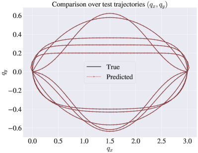
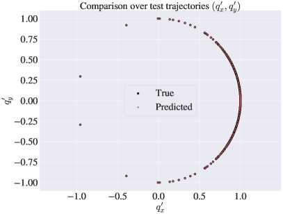
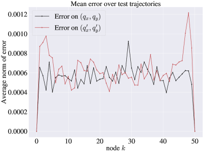
Figure 1: Comparison over test trajectories for $\mathbf{q}$ and $\mathbf{q}^{\prime}$ for the discrete network $q_{\boldsymbol{\rho}}^{\textrm{d}}$ tested on the both-ends data set with $90\%\--10\%$ splitting into training and test set. These results are obtained with the hyperparameters from Table 3, that yield a training error equal to $2.791\cdot 10^{-7}$ and a test error equal to $3.028\cdot 10^{-7}$ . For presentation purposes, only 10 randomly selected trajectories are considered in the first two plots.

As an additional evaluation of the deep learning framework’s behaviour, we conduct experiments to assess how the learning process performs when the number of training data varies, i.e., with different splittings of the data set into training and test sets. We report the results in Table 4 and summarise the corresponding hyperparameters in Table 12 of the Appendix.

$\begin{array}[]{c}\text{Data set splitting}\\ \text{Training \-- test}\end{array}$	Training accuracy	Test accuracy
10% - 10%	$6.530\cdot 10^{-5}$	$5.636\cdot 10^{-4}$
20% - 10%	$2.096\cdot 10^{-5}$	$3.457\cdot 10^{-5}$
40% - 10%	$2.186\cdot 10^{-6}$	$3.494\cdot 10^{-6}$
90% - 10%	$2.791\cdot 10^{-7}$	$3.028\cdot 10^{-7}$

Table 4: Behaviour of the discrete network $q_{\boldsymbol{\rho}}^{\textrm{d}}$ tested on the both-ends data set with fewer training data points. The size of the training set varies, while that of the test set is fixed. The last row corresponds to the results in Figure 1.

We also report results obtained by merging the both-end and the right-end trajectories, with $90\%\--10\%$ splitting of the whole new data set into training and test set. The results are shown in Figure 2 and the selected hyperparameters are collected in Table 5. The resulting training and test errors are, respectively, $3.047\cdot 10^{-7}$ and $3.141\cdot 10^{-7}$. Finally, we remark that the test accuracy is a good measure of the generalisation error of neural network under the hypothesis that the test and the training sets are independent of each other, but follow the same distribution. If we test over input boundary conditions that not only are unseen during the training, but also do not belong in the the same range of the training data, the resulting accuracy is expected to be low, since neural networks are in general not able to perform this sort of extrapolation. To show this, we consider the neural network trained and tested over the both-ends data set, related to the results in Figure 1 and in the last row of Table 4. We use 10% of the right-end data set as a test set, and we obtain a test error equal to $2.228\cdot 10^{-2}$. This highlights that care must be taken when using the trained network to make inference over new input data.

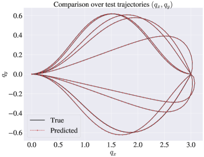
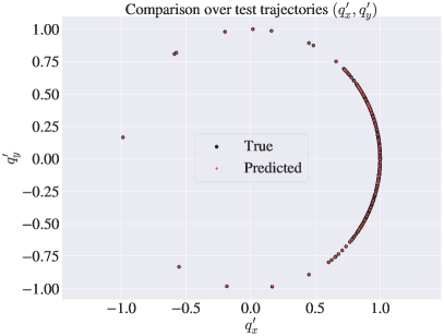
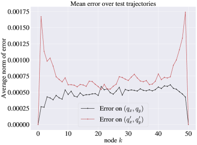
Figure 2: Comparison over test trajectories for $\mathbf{q}$ and $\mathbf{q}^{\prime}$ for the discrete network $q_{\boldsymbol{\rho}}^{\textrm{d}}$ tested on the both-ends + right-end data set with $90\%\--10\%$ splitting into training and test set. These results are obtained with the hyperparameters from Table 5, that yield a training error equal to $3.047\cdot 10^{-7}$ and a test error equal to $3.141\cdot 10^{-7}$. For presentation purposes, only 10 randomly selected trajectories are considered in the first two plots.

Selected hyperparameters
architecture	MLP
normalisation	True
activation function $\sigma$	LeakyReLU
#layers $\ell$	2
#hidden nodes in each layer	1006
learning rate $\eta$	$3.611\cdot 10^{-3}$
weight decay	$1.515\cdot 10^{-7}$
$\gamma$	$6.388\cdot 10^{-3}$
batch size	32

Table 5: Combination of hyperparameters yielding the best results for the discrete network $q_{\boldsymbol{\rho}}^{\textrm{d}}$ tested on the both-ends + right-end data set with $90\%\--10\%$ splitting into training and test set. The results are shown in Figure 2.

5 The continuous network

The approach described in the previous section shows accurate results, given a large enough amount of beam discretisations with a fixed number of nodes $N+1$, equally distributed in $[0,L]$. It seems reasonable to expect that the parametric model’s approximation quality improves when the number of discretisation nodes increases. However, in this approach, the dimension of the predicted vector grows with $N$, and hence minimising the loss function (11) becomes more difficult. In addition, the fact that the discrete network approach depends on the spatial discretisation of the training data restricts the output dimension to a specific number of nodes. Consequently, there would be two main options to assess the solution at different locations: training the network once more, or interpolating the previously obtained approximation. These limitations make such a discrete approach less appealing and suggest that having a neural network that is a smooth function of the arc length coordinate $s$ can be beneficial. This modelling assumption would also be compatible with different discretisations of the curve and would not suffer from the curse of dimensionality if more nodes were added. In this setting, the discrete node $s_{k}$ at which an approximation of the solution is available, is included in the input data together with the boundary conditions. As a result, we work with the following data set

$$\Omega=\left\{\left(s_{k},\,\mathbf{x}^{i}\right),\;{\mathbf{y}}_{k}^{i}\right\}_{k=0,\dots,N}^{i=1,\dots,M},$$

where, as in the previous section,

$$\mathbf{x}^{i}=\left(\,\mathbf{q}^{i}_{0},\,\mathbf{q}^{i}_{N},\,(\mathbf{q}^{i}_{0})^{\prime},\,(\mathbf{q}^{i}_{N})^{\prime}\right)\in\mathbb{R}^{8},$$

and

$${\mathbf{y}}_{k}^{i}=\left(\hat{\mathbf{q}}_{k}^{i},\,(\hat{\mathbf{q}}_{k}^{i})^{\prime}\right).$$

Here $\hat{\mathbf{q}}_{k}^{i}$ is the numerical solution $\hat{\mathbf{q}}$ on the node $s_{k}$, satisfying the $i$-th boundary conditions in Equation (10). Let us introduce the neural network

$$q_{\boldsymbol{\rho}}^{\mathrm{c}}:\mathbb{R}^{8}\to\mathcal{C}^{\infty}\left([0,L],\mathbb{R}^{2}\right),$$

and the differential operator

$$\mathcal{D}:\mathcal{C}^{\infty}\left([0,L],\mathbb{R}^{2}\right)\to\mathcal{C}^{\infty}\left([0,L],\mathbb{R}^{2}\right),\,\,\mathcal{D}\left(q_{\boldsymbol{\rho}}^{\mathrm{c}}\left(\mathbf{x}^{i}\right)\right)(s_{k})=\frac{d}{ds}\left(q_{\boldsymbol{\rho}}^{\rm c}(\boldsymbol{x}^{i})\right)(s)\Big{|}_{s=s_{k}},$$

so that we can define

$$y_{\boldsymbol{\rho}}\left(\mathbf{x}^{i}\right)(s_{k}):=\left(q_{\boldsymbol{\rho}}^{\mathrm{c}}\left(\mathbf{x}^{i}\right)(s_{k}),\,\mathcal{D}\left(q_{\boldsymbol{\rho}}^{\mathrm{c}}\left(\mathbf{x}^{i}\right)\right)(s_{k})\right).$$

To train the network $q_{\boldsymbol{\rho}}^{c}$, we define the loss function

$$\textrm{Loss}(\boldsymbol{\rho})=\frac{1}{4M(N+1)}\sum_{i=1}^{M}\sum_{k=0}^{N}\left(\left\|{y_{\boldsymbol{\rho}}}\left(\mathbf{x}^{i}\right)(s_{k})-{\boldsymbol{y}}_{k}^{i}\right\|^{2}_{2}+\gamma\left(\left\|\pi_{\mathcal{D}}\left(y_{\boldsymbol{\rho}}\left(\mathbf{x}^{i}\right)(s_{k})\right)\right\|_{2}^{2}-1\right)^{2}\right),$$ (12)

where $\pi_{\mathcal{D}}:\mathbb{R}^{8}\to\mathbb{R}^{4}$ is the projection on the second component $\mathcal{D}(q_{\boldsymbol{\rho}}^{\rm c}(\boldsymbol{x}^{i}))(s_{k})$, and $\gamma\geq 0$ weighs the violation of the normality constraint. The map $q_{\boldsymbol{\rho}}^{\textrm{c}}$ is now a neural network that associates each set of boundary conditions $\boldsymbol{x}^{i}$ with a smooth curve $q_{\boldsymbol{\rho}}^{\textrm{c}}\left(\boldsymbol{x}^{i}\right):[0,L]\to\mathbb{R}^{2}$ that can be evaluated at every point $s\in[0,L]$. We denote this network with the superscript $\mathrm{c}$, since this curve is in particular continuous. The outputs $q_{\boldsymbol{\rho}}^{\textrm{c}}\left(\boldsymbol{x}^{i}\right)(s)\in\mathbb{R}^{2}$ are approximations of the configuration of the beam at $s\in[0,L]$.

We point out that, contrarily to the discrete case, here we learn approximations of $\mathbf{q}(s)$ also on the end nodes, i.e., at $s=0$ and $s=L$. This is due to the fact that we do not impose the boundary conditions by construction. Even though there are multiple approaches to embed them into the network architecture, the one we try in our experiments made the optimisation problem too difficult, thus we only impose the boundary conditions weakly in the loss function.

Another strategy is to compute the angles $\theta_{k}$ between the tangents $(\hat{\mathbf{q}}_{k})^{\prime}$ and the $x$-axis and to use them as training data. To this end, we define the neural network

$$\theta_{\boldsymbol{\rho}}^{\textrm{c}}:\mathbb{R}^{8}\to\mathcal{C}^{\infty}\left([0,L],\mathbb{R}\right)$$

as $\theta_{\boldsymbol{\rho}}^{\textrm{c}}=\hat{\theta}_{\boldsymbol{\rho}}^{\textrm{c}}\circ\pi$, where

$$\hat{\theta}_{\boldsymbol{\rho}}^{\textrm{c}}:\mathbb{R}^{2}\to\mathcal{C}^{\infty}\left([0,L],\mathbb{R}\right)$$ (13)

is a neural network and the function $\pi:\mathbb{R}^{8}\to\mathbb{R}^{2}$ extracts the tangential angles from the boundary conditions, i.e., $\pi\left(\boldsymbol{x}^{i}\right)=\left(\theta_{0}^{i},\theta_{N}^{i}\right)$. Such a network should approximate the angular function $\theta:[0,L]\ni s\to\mathbb{R}$, so that

$$\tau_{\boldsymbol{\rho}}^{\mathrm{c}}\left(\boldsymbol{x}^{i}\right)(s):=\left(\cos\left(\theta_{\boldsymbol{\rho}}^{\textrm{c}}\left(\boldsymbol{x}^{i}\right)(s)\right),\sin\left(\theta_{\boldsymbol{\rho}}^{\textrm{c}}\left(\boldsymbol{x}^{i}\right)(s)\right)\right)\in\mathbb{R}^{2}$$ (14)

gets close to the tangent vector $\mathbf{q}^{\prime}(s)$. As a result, the constraint on the unit norm of the tangents is satisfied by construction, and the inextensibility of the elastica is guaranteed. The curve

$$\mathbf{q}(s)=\mathbf{q}_{0}+\int_{0}^{s}\mathbf{q}^{\prime}(\bar{s})\mathrm{d}\bar{s}$$

can then be approximated through the reconstruction formula

$$q_{\boldsymbol{\rho}}^{\textrm{c}}\left(\boldsymbol{x}^{i}\right)(s)=\mathbf{q}_{0}+\mathcal{I}\left(\tau_{\rho}^{\mathrm{c}}\left(\boldsymbol{x}^{i}\right)\right)(s),$$ (15)

where the operator $\mathcal{I}:\mathcal{C}^{\infty}\left([0,L],\mathbb{R}^{2}\right)\to\mathcal{C}^{\infty}\left([0,L],\mathbb{R}^{2}\right)$ is such that

$$\mathcal{I}\left(\tau_{\rho}^{\mathrm{c}}\left(\boldsymbol{x}^{i}\right)\right)(s)\approx\int_{0}^{s}\tau_{\rho}^{\mathrm{c}}\left(\mathbf{x}^{i}\right)(\bar{s})\mathrm{d}\bar{s}.$$

In the numerical experiments, $\mathcal{I}$ is based on the $3$-point Gaussian quadrature formula applied to a partition of the interval $[0,L]$, see [7, Chapter 9]. As done previously, we define the vector

$$y_{\boldsymbol{\rho}}\left(\mathbf{x}^{i}\right)(s_{k}):=\left(q_{\boldsymbol{\rho}}^{\mathrm{c}}\left(\mathbf{x}^{i}\right)(s_{k}),\,\tau_{\boldsymbol{\rho}}^{\rm c}\left(\boldsymbol{x}^{i}\right)(s_{k})\right),$$ (16)

with components defined as in Equations (14) and (15). This allows us to train the network $\theta_{\boldsymbol{\rho}}^{\rm c}$ by minimising the same loss function as in Equation (12), where this time $y_{\boldsymbol{\rho}}^{\rm c}$ is given by Equation (16). Furthermore, since by construction this case satisfies $\left\|\pi_{\mathcal{D}}\left(y_{\boldsymbol{\rho}}^{\rm c}(\boldsymbol{x}^{i})(s)\right)\right\|_{2}=\left\|\tau_{\boldsymbol{\rho}}^{\mathrm{c}}\left(\boldsymbol{x}^{i}\right)(s)\right\|_{2}\equiv 1$, we set $\gamma=0$. We present numerical experiments for the two proposed continuous networks $q_{\boldsymbol{\rho}}^{\textrm{c}}$ and $\theta_{\boldsymbol{\rho}}^{\textrm{c}}$. In the latter case, by neural network architecture we refer to $\hat{\theta}_{\boldsymbol{\rho}}^{\rm c}$ rather than $\theta_{\boldsymbol{\rho}}^{\rm c}$ in what follows. We analyse $q_{\boldsymbol{\rho}}^{\textrm{c}}$ more thoroughly in Section 5.1, mirroring most of the discrete case experiments. In Section 5.2 we study how the results are affected when we impose the arc length parametrization and enforce the boundary conditions to be exactly satisfied by the network $\theta_{\boldsymbol{\rho}}^{\textrm{c}}$.

5.1 Numerical experiments with $q_{\boldsymbol{\rho}}^{\textrm{c}}$

As for the case of the discrete network, we perform an in-depth investigation of this learning setting by varying the architecture of the continuous neural network and the hyperparameters in the training procedure, whose range of options can be found in Table 6. In this case, we define the loss as in Equation (12), with $\gamma=10^{-2}$. The weight decay is systematically set to $0$.

Hyperparameter	Range	Distribution
architecture	{MLP, ResNet, MULT}	discrete uniform
normalisation	{True, False}	discrete uniform
activation function $\sigma$	{Tanh, Swish, Sigmoid, Sine}	discrete uniform
#layers $\ell$	$\{3,\ldots,8\}$	discrete uniform
#hidden nodes in each layer	$[10,200]\cap\mathbb{N}$	discrete uniform
learning rate $\eta$	$[1\cdot 10^{-4},1\cdot 10^{-1}]$	log uniform

Table 6: Hyperparameter ranges for the continuous network $q_{\boldsymbol{\rho}}^{\textrm{c}}$ tested on the both-ends data set with $90\%\--10\%$ splitting into training and test set. The first column of the table reports the hyperparameters and network architectures we test for. The second describes the set of allowed values for each, while the third specifies how such values are explored through Optuna. The weight decay is systematically set to $0$. MULT stands for multiplicative neural network and corresponds to the network in Equations (20)-(24) of Appendix A.

Table 7 collects the combination of hyperparameters yielding the best results on the both-ends data set. This leads to a training error equal to $1.869\cdot 10^{-6}$ and a test error equal to $4.81\cdot 10^{-6}$. In Figure 3, the comparison over test trajectories for $\mathbf{q}$ and $\mathbf{q}^{\prime}$ is shown. As we can see in the plot showing the mean error over the trajectories, the error on the end nodes is nonzero, since we are not imposing boundary conditions by construction. This is in contrast to the corresponding plot for the discrete network in Figure 1.

Selected hyperparameters
architecture	MULT
normalisation	True
activation function $\sigma$	Tanh
#layers $\ell$	5
#hidden nodes in each layer	190
learning rate $\eta$	$3.025\cdot 10^{-3}$

Table 7: Combination of hyperparameters yielding the best results for the continuous network $q_{\boldsymbol{\rho}}^{\textrm{c}}$ tested on the both-ends data set with $90\%\--10\%$ splitting into training and test set. The results are shown in Figure 3.

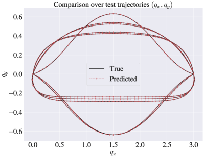
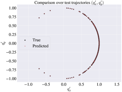
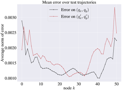
Figure 3: Comparison over test trajectories for $\mathbf{q}$ and $\mathbf{q}^{\prime}$ for the continuous network $q_{\boldsymbol{\rho}}^{\textrm{c}}$ tested on the both-ends data set with $90\%\--10\%$ splitting into training and test set. These results are obtained with the hyperparameters from Table 7, that yield a training error equal to $1.869\cdot 10^{-6}$ and a test error equal to $4.810\cdot 10^{-6}$. For presentation purposes, only 10 randomly selected trajectories are considered in the first two plots.

Also in this case, we examine the behaviour of the learning process with different splittings of the data set into training and test sets. We display the results in Table 8 and summarise the corresponding hyperparameters in Appendix B, Table 13.

$\begin{array}[]{c}\text{Data set splitting}\\ \text{Training \-- test}\end{array}$	Training accuracy	Test accuracy
10% - 10%	$2.383\cdot 10^{-4}$	$7.784\cdot 10^{-4}$
20% - 10%	$5.612\cdot 10^{-5}$	$7.285\cdot 10^{-5}$
40% - 10%	$7.104\cdot 10^{-6}$	$9.275\cdot 10^{-6}$
90% - 10%	$1.869\cdot 10^{-6}$	$4.810\cdot 10^{-6}$

Table 8: Behaviour of the continuous network $q_{\boldsymbol{\rho}}^{\textrm{c}}$ tested on the both-ends data set with fewer training data points. The size of the training set varies, while that of the test set is fixed. The last row corresponds to the results in Figure 3.

5.2 Numerical experiments with $\theta_{\boldsymbol{\rho}}^{\textrm{c}}$

Here we consider a neural network approximation of the angle $\theta(s)$ that parametrises the tangent vector $\mathbf{q}^{\prime}(s)=(\cos(\theta(s)),\sin(\theta(s)))$. By design, the approximation $\tau_{\boldsymbol{\rho}}^{\mathrm{c}}$ of the tangent vector $\mathbf{q}^{\prime}$ satisfies the constraint $\|\tau_{\boldsymbol{\rho}}^{\mathrm{c}}(\boldsymbol{x}^{i})(s)\|_{2}=1$ for every $s\in[0,L]$ and $\boldsymbol{x}^{i}\in\mathbb{R}^{8}$. We also analyse how the neural network approximation behaves when the boundary conditions $\tau_{\boldsymbol{\rho}}^{\mathrm{c}}(\boldsymbol{x}^{i})(0)=\mathbf{q}^{\prime}(0)$ and $\tau_{\boldsymbol{\rho}}^{\mathrm{c}}(\boldsymbol{x}^{i})(L)=\mathbf{q}^{\prime}(L)$ are imposed by construction. To do so, we model the parametric function $\hat{\theta}_{\boldsymbol{\rho}}^{\textrm{c}}$, defined in Equation (13), in one of the two following ways:

$$\hat{\theta}_{\boldsymbol{\rho}}^{\textrm{c}}(\boldsymbol{x}^{i})(s)=f_{\boldsymbol{\rho}}(s,\theta_{0}^{i},\theta_{N}^{i}),$$ (17)

$$\begin{split}\hat{\theta}_{\boldsymbol{\rho}}^{\textrm{c}}(\boldsymbol{x}^{i})(s)&=f_{\boldsymbol{\rho}}(s,\theta_{0}^{i},\theta_{N}^{i})+(\theta_{0}^{i}-f_{\boldsymbol{\rho}}(0,\theta_{0}^{i},\theta_{N}^{i}))e^{-100s^{2}}\\ &+(\theta_{N}^{i}-f_{\boldsymbol{\rho}}(L,\theta_{0}^{i},\theta_{N}^{i}))e^{-100(s-L)^{2}},\end{split}$$ (18)

where $f_{\boldsymbol{\rho}}:\mathbb{R}^{3}\to\mathbb{R}$ is any neural network, and we recall that $\pi(\boldsymbol{x}^{i})=(\theta_{0}^{i},\theta_{N}^{i})$. We remark that, in the case of the parameterisation in Equation (18), one gets $\theta_{\boldsymbol{\rho}}^{\textrm{c}}(\boldsymbol{x}^{i})(0)=\theta_{0}^{i}$ and $\theta_{\boldsymbol{\rho}}^{\textrm{c}}(\boldsymbol{x}^{i})(L)=\theta_{N}^{i}$ up to machine precision, due to the fast decay of the Gaussian function. As in the previous sections, we collect the hyperparameter and architecture options with the respective range of choices in Table 9, and we report the results without imposing the boundary conditions in Figure 4, while those imposing them in Figure 5, in both cases using the both-ends data set, with $90\%\--10\%$ splitting into training and test set. The results shown in the two figures correspond respectively to training errors of $5.821\cdot 10^{-6}$ and $6.068\cdot 10^{-6}$, and test errors of $6.231\cdot 10^{-6}$ and $6.289\cdot 10^{-6}$. The best performing hyperparameter combinations can be found in Tables 10 and 11.

Hyperparameter	Range	Distribution
architecture	{MLP, ResNet, MULT}	discrete uniform
activation function $\sigma$	{Tanh, Swish, Sigmoid}	discrete uniform
#layers $\ell$	$\{3,\ldots,8\}$	discrete uniform
#hidden nodes in each layer	$[50,200]\cap\mathbb{N}$	discrete uniform
learning rate $\eta$	$[1\cdot 10^{-3},1\cdot 10^{-1}]$	log uniform

Table 9: Hyperparameter ranges for the continuous network $\theta_{\boldsymbol{\rho}}^{\textrm{c}}$ tested on the both-ends data set. The first column of the table reports the hyperparameters and network architectures we test for. The second describes the set of allowed values for each, while the third specifies how such values are explored through Optuna. The weight decay is systematically set to $0$, and no normalisation is applied.

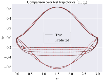
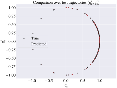
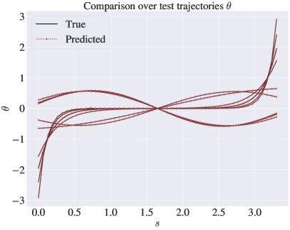
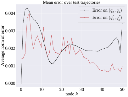
Figure 4: Comparison over test trajectories for $\mathbf{q}$ and $\mathbf{q}^{\prime}$, for the case $\theta_{\boldsymbol{\rho}}^{\textrm{c}}$ is modelled as in Equation (17), with $90\%\--10\%$ splitting of the both-ends data set into training and test set. These results are obtained with the hyperparameters from Table 10, that yield a training error equal to $5.821\cdot 10^{-6}$ and a test error equal to $6.231\cdot 10^{-6}$. For presentation purposes, only 10 randomly selected trajectories are considered in the first two plots.

Selected hyperparameters
architecture	MULT
activation function $\sigma$	Tanh
#layers $\ell$	$7$
#hidden nodes in each layer	$143$
learning rate $\eta$	$3.007\cdot 10^{-3}$

Table 10: Combination of hyperparameters yielding the best results for the case when $\theta_{\boldsymbol{\rho}}^{\textrm{c}}$ is modelled as in Equation (17), with $90\%\--10\%$ splitting of the both-ends data set into training and test set. The results are shown in Figure 4.

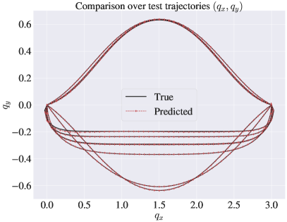
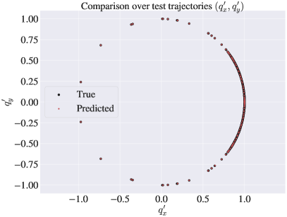
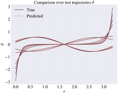
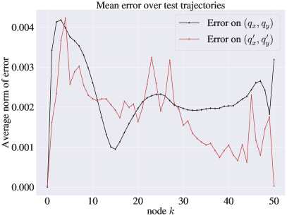
Figure 5: Comparison over test trajectories for $\mathbf{q}$ and $\mathbf{q}^{\prime}$, for the case $\theta_{\boldsymbol{\rho}}^{\textrm{c}}$ is modelled as in Equation (18), with $90\%\--10\%$ splitting of the both-ends data set into training and test set. These results are obtained with the hyperparameters from Table 11, that yield a training error equal to $6.068\cdot 10^{-6}$ and a test error equal to $6.289\cdot 10^{-6}$. For presentation purposes, only 10 randomly selected trajectories are considered in the first two plots.

Selected hyperparameters
architecture	MULT
activation function $\sigma$	Tanh
#layers $\ell$	$4$
#hidden nodes in each layer	$175$
learning rate $\eta$	$1.846\cdot 10^{-3}$

Table 11: Combination of hyperparameters yielding the best results for the case when $\theta_{\boldsymbol{\rho}}^{\textrm{c}}$ is modelled as in Equation (18), with $90\%\--10\%$ splitting of the both-ends data set into training and test set. The results are shown in Figure 5.

6 Discussion

The results in Figures 4 and 5 are comparable, especially looking at the mean error plots. This suggests that the imposition of the boundary conditions, in the proposed way, is not limiting the expressivity of the considered network. Thus, given the boundary value nature of our problem, these figures advocate the enforcement of the boundary conditions on the network $\theta_{\boldsymbol{\rho}}^{\textrm{c}}$. However, due to the chosen reconstruction procedure in Equation (15) for the variable $\mathbf{q}$, we are able to impose the boundary conditions on $\mathbf{q}$ only on the left node. Clearly, other more symmetric reconstruction procedures can be adopted, but the proposed one has proved to provide better experimental results.

Comparing the results related to $q_{\boldsymbol{\rho}}^{\textrm{c}}$ with those of $\theta_{\boldsymbol{\rho}}^{\textrm{c}}$, we notice similar performances in terms of training and test errors. In both the cases, they have one order of magnitude more than the corresponding training and test errors of the discrete network $q_{\boldsymbol{\rho}}^{\textrm{d}}$. Thus, as a results of our experiments, we can conclude that

• if the accuracy and the efficient evaluation of the model at the discrete nodes are of interest, the discrete network is the best option;

• for a more flexible model, not restricted to the discrete nodes, the continuous network is a better choice; among the two proposed modelling strategies, working with $q_{\boldsymbol{\rho}}^{\textrm{c}}$ is more suitable for an easy parametrisation of both $\mathbf{q}$ and $\mathbf{q}^{\prime}$, while $\theta_{\boldsymbol{\rho}}^{\textrm{c}}$ is more suitable to impose geometrical structure and constraints.

The total accuracy error of a neural network model can be defined by splitting it into three components: approximation error, optimisation error, and generalisation error (see, e.g., [17]). To achieve excellent agreement between predicted and reference trajectories, it is important to select the appropriate architecture and fine-tune the model hyperparameters. Our results demonstrate that we can construct a network that is expressive enough to provide a small approximation error and with very good generalisation capability.

6.1 Future work

In the methods presented in this paper, there is no interaction between the mathematical problem and the neural network model once the data set is created. As a way to improve the results presented here, one could include the Euler elastica model directly into the training process. This could be done either by directly imposing in the loss function that $\mathbf{q}(s)$ satisfies the differential equations (5), or one could add the constrained action integral from Equation (4) into the loss function that is minimised, see e.g. [28, 10, 12, 11].

There are many promising directions in order to follow up this work. One is to consider 3D versions of the Euler elastica, another is to look at the dynamical problem, and finally one may examine industrial applications. As an example, we refer to the modelling of endoscopes due to the high bending deformation of these medical devices under certain loading cases [30]. The approximation of the elastica through neural networks can indeed help in the prediction of the deformed configuration of the beam in constrained narrow environments.

Acknowledgments. This project has received funding from the European Union’s Horizon 2020 research and innovation programme under the Marie Skłodowska-Curie grant agreement No 860124. This work was partially supported by a grant from the Simons Foundation (DM). This contribution reflects only the authors’ view, and the Research Executive Agency and the European Commission are not responsible for any use that may be made of the information it contains.

Appendix A Other neural network architectures

Another example of neural network architecture, besides the MLP defined in Equation (9), is the residual neural network (ResNet), where

$$f_{j}^{RES}(\mathbf{x})=\mathbf{x}+\mathbf{B}_{j}^{T}\sigma(\mathbf{A}_{j}\mathbf{x}+\mathbf{b}_{j})\in\mathbb{R}^{n},$$ (19)

with $\mathbf{x}\in\mathbb{R}^{n}$, $\mathbf{A}_{j},\mathbf{B}_{j}\in\mathbb{R}^{n_{j}\times n}$, $\mathbf{b}_{j}\in\mathbb{R}^{n_{j}}$, and $\boldsymbol{\rho}=\{\mathbf{A}_{j},\mathbf{b}_{j},\mathbf{B}_{j}\}_{j=1}^{\ell}$.

We also provide the expression of the forward propagation of the multiplicative network used for the experiments in Section 5:

$$\mathbf{U}=\sigma(\mathbf{W}_{1}\mathbf{x}+\mathbf{b}_{1}),\quad\mathbf{V}=\phi(\mathbf{W}_{2}\mathbf{x}+\mathbf{b}_{2})$$ (20)

$$\mathbf{H}_{1}=\sigma(\mathbf{W}_{3}\mathbf{x}+\mathbf{b}_{3})$$ (21)

$$\mathbf{Z}_{j}=\sigma(\mathbf{W}^{z}_{j}\mathbf{H}_{j}+\mathbf{b}^{z}_{j}),\;j=1,\dots,\ell$$ (22)

$$\mathbf{H}_{j+1}=(1-\mathbf{Z}_{j})\odot\mathbf{U}+\mathbf{Z}_{j}\odot\mathbf{V},\;j=1,\dots,\ell$$ (23)

$$f_{\boldsymbol{\rho}}^{MULT}(\mathbf{x})=\mathbf{W}\mathbf{H}_{\ell+1}+\mathbf{b},$$ (24)

where $\odot$ denotes the component-wise multiplications. In this case, $\boldsymbol{\rho}=\left\{\mathbf{W}_{1},\mathbf{b}_{1},\mathbf{W}_{2},\mathbf{b}_{2},\mathbf{W}_{3},\mathbf{b}_{3},\left(\mathbf{W}^{z}_{j},\mathbf{b}^{z}_{j}\right)_{j=1}^{\ell},\mathbf{W},\mathbf{b}\right\}$, and the weight matrices and biases have shapes that allow for the expressions (20)-(24) to be well-defined. This architecture is inspired by neural attention mechanisms and was introduced in [47] to improve the gradient behaviour. A further motivation for our choice of including this architecture is experimental since it has proven effective in solving the task of interest, while still having a similar number of parameters to the MLP architecture. Throughout the paper, we refer to this architecture as multiplicative since it includes component-wise multiplications, which help capture multiplicative interactions between the variables.

Appendix B Further results on the hyperparameters of the neural networks

$\begin{array}[]{c}\text{Hyperparameter}\\ \text{combination}\end{array}$	Data set splitting
	10% - 10%	20% - 10%	40% - 10%	90% - 10%
architecture	MLP	MLP	MLP	MLP
normalization	False	False	False	True
activation function $\sigma$	Tanh	Tanh	Tanh	Tanh
number of layers $\ell$	4	4	3	4
#hidden nodes in each layer	950	351	904	879
learning rate $\eta$	$1.019\cdot 10^{-3}$	$5.455\cdot 10^{-3}$	$1.429\cdot 10^{-3}$	$1.378\cdot 10^{-3}$
weight decay	$1.79\cdot 10^{-6}$	$2.142\cdot 10^{-7}$	$1.317\cdot 10^{-7}$	$1.535\cdot 10^{-7}$
$\gamma$	$8.595\cdot 10^{-3}$	$2.973\cdot 10^{-3}$	$9.338\cdot 10^{-3}$	$4.242\cdot 10^{-3}$
batch size	64	32	32	32

Table 12: Choice of hyperparameters for the training of the discrete network $q_{\boldsymbol{\rho}}^{\textrm{d}}$ tested on the both-ends data set with different numbers of training data points.

$\begin{array}[]{c}\text{Hyperparameter}\\ \text{combination}\end{array}$	Data set splitting
	10% - 10%	20% - 10%	40% - 10%	90% - 10%
architecture	MULT	MULT	MULT	MULT
normalization	True	True	True	True
activation function $\sigma$	Tanh	Tanh	Sine	Tanh
number of layers $\ell$	5	6	6	5
#hidden nodes in each layer	193	121	169	190
learning rate $\eta$	$4.548\cdot 10^{-3}$	$4.913\cdot 10^{-3}$	$4.2\cdot 10^{-3}$	$3.025\cdot 10^{-3}$

Table 13: Choice of hyperparameters for the training of the continuous network $q_{\boldsymbol{\rho}}^{\textrm{c}}$ tested on the both-ends data set with different numbers of training data points. The weight decay is systematically set to 0.

References

- \bibcommenthead
- [1] Saad, Y.: Iterative Methods for Sparse Linear Systems. SIAM, (2003)
- [2] Nocedal, J., Wright, S.J.: Numerical Optimization. Springer, (1999)
- Marsden and West [2001] Marsden, J.E., West, M.: Discrete mechanics and variational integrators. Acta numerica 10, 357–514 (2001)
- [4] Hairer, E., Nørsett, S.P., Wanner, G.: Solving Ordinary Differential Equations I, Nonstiff Problems, Second revised edition edn. Springer, (1993)
- [5] Hairer, E., Wanner, G.: Solving Ordinary Differential Equations II, Stiff and Differential-Algebraic Problems, Second revised edition edn. Springer, (1996)
- [6] Brenner, S.C.: The Mathematical Theory of Finite Element Methods. Springer, (2008)
- [7] Quarteroni, A., Sacco, R., Saleri, F.: Numerical Mathematics vol. 37. Springer, (2006)
- Cuomo et al. [2022] Cuomo, S., Di Cola, V.S., Giampaolo, F., Rozza, G., Raissi, M., Piccialli, F.: Scientific machine learning through physics–informed neural networks: Where we are and what’s next. Journal of Scientific Computing 92(3), 88 (2022)
- Brunton and Kutz [2023] Brunton, S.L., Kutz, J.N.: Machine learning for partial differential equations. arXiv:2303.17078 (2023)
- Raissi et al. [2019] Raissi, M., Perdikaris, P., Karniadakis, G.E.: Physics-informed neural networks: A deep learning framework for solving forward and inverse problems involving nonlinear partial differential equations. Journal of Computational physics 378, 686–707 (2019)
- Samaniego et al. [2020] Samaniego, E., Anitescu, C., Goswami, S., Nguyen-Thanh, V.M., Guo, H., Hamdia, K., Zhuang, X., Rabczuk, T.: An energy approach to the solution of partial differential equations in computational mechanics via machine learning: Concepts, implementation and applications. Computer Methods in Applied Mechanics and Engineering 362, 112790 (2020)
- E and Yu [2018] E, W., Yu, B.: The Deep Ritz Method: A Deep Learning-Based Numerical Algorithm for Solving Variational Problems. Communications in Mathematics and Statistics 6(1), 1–12 (2018)
- Gu and Ng [2023] Gu, Y., Ng, M.K.: Deep neural networks for solving large linear systems arising from high-dimensional problems. SIAM Journal on Scientific Computing 45(5), 2356–2381 (2023)
- Kadupitiya et al. [2022] Kadupitiya, J., Fox, G.C., Jadhao, V.: Solving Newton’s equations of motion with large timesteps using recurrent neural networks based operators. Machine Learning: Science and Technology 3(2), 025002 (2022)
- Liu et al. [2020] Liu, Y., Kutz, J., Brunton, S.: Hierarchical deep learning of multiscale differential equation time-steppers, arxiv. arXiv:2008.09768 (2020)
- Mattheakis et al. [2022] Mattheakis, M., Sondak, D., Dogra, A.S., Protopapas, P.: Hamiltonian neural networks for solving equations of motion. Physical Review E 105(6), 065305 (2022)
- Lu et al. [2021a] Lu, L., Jin, P., Pang, G., Zhang, Z., Karniadakis, G.E.: Learning nonlinear operators via deeponet based on the universal approximation theorem of operators. Nature machine intelligence 3(3), 218–229 (2021)
- Lu et al. [2021b] Lu, L., Meng, X., Mao, Z., Karniadakis, G.E.: Deepxde: A deep learning library for solving differential equations. SIAM review 63(1), 208–228 (2021)
- Chevalier et al. [2022] Chevalier, S., Stiasny, J., Chatzivasileiadis, S.: Accelerating dynamical system simulations with contracting and physics-projected neural-newton solvers. In: Learning for Dynamics and Control Conference, PMLR, pp. 803–816 (2022)
- Li et al. [2022] Li, Y., Zhou, Z., Ying, S.: Delisa: Deep learning based iteration scheme approximation for solving pdes. Journal of Computational Physics 451, 110884 (2022)
- Schiassi et al. [2021] Schiassi, E., Furfaro, R., Leake, C., De Florio, M., Johnston, H., Mortari, D.: Extreme theory of functional connections: A fast physics-informed neural network method for solving ordinary and partial differential equations. Neurocomputing 457, 334–356 (2021)
- De Florio et al. [2022] De Florio, M., Schiassi, E., Furfaro, R.: Physics-informed neural networks and functional interpolation for stiff chemical kinetics. Chaos: An Interdisciplinary Journal of Nonlinear Science 32(6) (2022)
- Fabiani et al. [2023] Fabiani, G., Galaris, E., Russo, L., Siettos, C.: Parsimonious physics-informed random projection neural networks for initial value problems of ODEs and index-1 DAEs. Chaos: An Interdisciplinary Journal of Nonlinear Science 33(4) (2023)
- Mortari et al. [2019] Mortari, D., Johnston, H., Smith, L.: High accuracy least-squares solutions of nonlinear differential equations. Journal of computational and applied mathematics 352, 293–307 (2019)
- [25] Kollmannsberger, S., D’Angella, D., Jokeit, M., Herrmann, L.: Deep Learning in Computational Mechanics. Springer, (2021)
- [26] Yagawa, G., Oishi, A.: Computational Mechanics with Deep Learning: An Introduction. Springer, (2022)
- Loc Vu-Quoc [2023] Loc Vu-Quoc, A.H.: Deep learning applied to computational mechanics: A comprehensive review, state of the art, and the classics. Computer Modeling in Engineering & Sciences 137(2), 1069–1343 (2023)
- Lagaris et al. [1998] Lagaris, I.E., Likas, A., Fotiadis, D.I.: Artificial neural networks for solving ordinary and partial differential equations. IEEE transactions on neural networks 9(5), 987–1000 (1998)
- Ntarladima et al. [2023] Ntarladima, K., Pieber, M., Gerstmayr, J.: A model for contact and friction between beams under large deformation and sheaves. Nonlinear Dynamics, 1–18 (2023)
- Stavole et al. [2022] Stavole, M., Almagro, R.T.S.M., Lohk, M., Leyendecker, S.: Homogenization of the constitutive properties of composite beam cross-sections. In: ECCOMAS Congress 2022-8th European Congress on Computational Methods in Applied Sciences and Engineering (2022)
- Manfredo et al. [2023] Manfredo, D., Dörlich, V., Linn, J., Arnold, M.: Data based constitutive modelling of rate independent inelastic effects in composite cables using preisach hysteresis operators. Multibody System Dynamics, 1–16 (2023)
- Saadat and Durville [2023] Saadat, M.A., Durville, D.: A mixed stress-strain driven computational homogenization of spiral strands. Computers & Structures 279, 106981 (2023)
- Euler [1744] Euler, L.: De Curvis Elastici. Additamentum in Methodus inveniendi lineas curvas maximi minimive proprietate gaudentes, sive solutio problematis isoperimetrici lattissimo sensu accepti, Lausanne (1744)
- Love [1863 - 1940] Love, A.E.H.: A Treatise on the Mathematical Theory of Elasticity. Cambridge University Press, Cambridge (1863 - 1940)
- Matsutani [2010] Matsutani, S.: Euler’s elastica and beyond. Journal of Geometry and Symmetry in Physics 17, 45–86 (2010)
- Singer [2008] Singer, D.A.: Lectures on elastic curves and rods. In: AIP Conference Proceedings, vol. 1002. American Institute of Physics, pp. 3–32 (2008)
- Rohrhofer et al. [2022] Rohrhofer, F.M., Posch, S., Gößnitzer, C., Geiger, B.C.: On the role of fixed points of dynamical systems in training physics-informed neural networks. Transactions on Machine Learning Research (2022)
- Colombo et al. [2016] Colombo, L., Ferraro, S., Diego, D.: Geometric integrators for higher-order variational systems and their application to optimal control. Journal of Nonlinear Science 26, 1615–1650 (2016)
- Ferraro et al. [2021] Ferraro, S.J., Diego, D.M., Almagro, R.T.S.M.: Parallel iterative methods for variational integration applied to navigation problems. IFAC-PapersOnLine 54(19), 321–326 (2021)
- [40] Timoshenko, S.P., Gere, J.M.: Theory of Elastic Stability. McGraw-Hill Book Company, (1961)
- [41] Bigoni, D.: Nonlinear Solid Mechanics: Bifurcation Theory and Material Instability. Cambridge University Press, (2012)
- Virtanen et al. [2020] Virtanen, P., Gommers, R., Oliphant, T.E., Haberland, M., Reddy, T., Cournapeau, D., Burovski, E., Peterson, P., Weckesser, W., Bright, J., van der Walt, S.J., Brett, M., Wilson, J., Millman, K.J., Mayorov, N., Nelson, A.R.J., Jones, E., Kern, R., Larson, E., Carey, C.J., Polat, İ., Feng, Y., Moore, E.W., VanderPlas, J., Laxalde, D., Perktold, J., Cimrman, R., Henriksen, I., Quintero, E.A., Harris, C.R., Archibald, A.M., Ribeiro, A.H., Pedregosa, F., van Mulbregt, P., SciPy 1.0 Contributors: SciPy 1.0: Fundamental Algorithms for Scientific Computing in Python. Nature Methods 17, 261–272 (2020)
- Higham and Higham [2019] Higham, C.F., Higham, D.J.: Deep learning: An introduction for applied mathematicians. Siam review 61(4), 860–891 (2019)
- Kingma and Ba [2015] Kingma, D., Ba, J.: Adam: A method for stochastic optimization. In: International Conference on Learning Representations (ICLR), San Diega, CA, USA (2015)
- Paszke et al. [2019] Paszke, A., Gross, S., Massa, F., Lerer, A., Bradbury, J., Chanan, G., Killeen, T., Lin, Z., Gimelshein, N., Antiga, L., et al.: Pytorch: An imperative style, high-performance deep learning library. Advances in neural information processing systems 32 (2019)
- Akiba et al. [2019] Akiba, T., Sano, S., Yanase, T., Ohta, T., Koyama, M.: Optuna: A next-generation hyperparameter optimization framework. In: Proceedings of the 25th ACM SIGKDD International Conference on Knowledge Discovery and Data Mining, pp. 2623–2631 (2019)
- Wang et al. [2021] Wang, S., Teng, Y., Perdikaris, P.: Understanding and mitigating gradient flow pathologies in physics-informed neural networks. SIAM Journal on Scientific Computing 43(5), 3055–3081 (2021)