RefinedFields: Radiance Fields Refinement for Unconstrained Scenes

Abstract

Modeling large scenes from unconstrained images has proven to be a major challenge in computer vision. Existing methods tackling in-the-wild scene modeling operate in closed-world settings, where no conditioning on priors acquired from real-world images is present. We propose RefinedFields, which is, to the best of our knowledge, the first method leveraging pre-trained models to improve in-the-wild scene modeling. We employ pre-trained networks to refine K-Planes representations via optimization guidance using an alternating training procedure. We carry out extensive experiments and verify the merit of our method on synthetic data and real tourism photo collections. RefinedFields enhances rendered scenes with richer details and outperforms previous work on the task of novel view synthesis in the wild. Our project page can be found at https://refinedfields.github.io .

1 Introduction

To draw novel objects and views, humans often rely on a blend of cognition and intuition, where the latter is built on a large prior acquired from a long-term continuous exploration of the visual world. Nevertheless, ablating one of these two elements results in catastrophic representations. On the one hand, humans find it particularly difficult to draw a bicycle based solely on this preconceived prior (Gimini, 2016). However, once one photograph is observed, drawing novel views of a bicycle becomes straightforward. On the other hand, drawing monuments and complex objects based solely on observed images, and with no preconceived notions of geometry and physics, is also non-trivial. In computer vision, recent methods tackling object generation and novel view synthesis are exclusively built on either the former or the latter ablation.

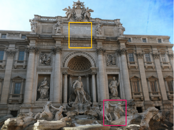
(a)

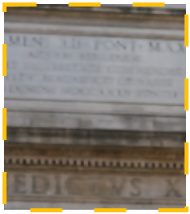
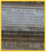
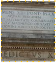
(b)

[K-Planes]

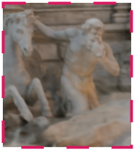
[RefinedFields]

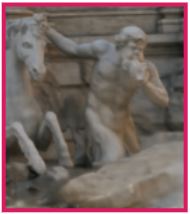
[GT]

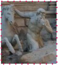
(a)

Figure 1: Qualitative Results. Given images of the Trevi fountain from Phototourism (Jin et al., 2020), as well as a pre-trained model (Rombach et al., 2022), our method leverages the pre-trained model and refines K-Planes with finer details that are under-represented when optimizing the same K-Planes on the images alone.

The first class of methods approaches novel view synthesis by learning scenes through rigorous cognition, as in dense observations of captured images. Although classic methodologies like structure-from-motion (Hartley & Zisserman, 2004) and image-based rendering (Shum et al., 2008) have previously tackled this problem, the field has recently seen substantial advancements thanks to neural representations coupled with volume rendering techniques (Mildenhall et al., 2020; Chan et al., 2022). Recent methods extend NeRFs (Martin-Brualla et al., 2021; Chen et al., 2022b; Yang et al., 2023) and Tri-Planes (Fridovich-Keil et al., 2023) to support learning from unconstrained “in-the-wild” photo collections by enabling robustness against illumination variations and transient occluders. These representations, however, do not learn any prior across scenes as they are trained from scratch for each scene. This means that these representations are learned in a closed-world setting, where the information scope is limited to the training set at hand.

Table 1: Related work overview. RefinedFields leverages unconstrained tourist photo collections (Jin et al., 2020) and a pre-trained prior (Rombach et al., 2022) to refine K-Planes, our underlying scene representation, in order to achieve state-of-the-art performance in in-the-wild scene modeling. Due to size constraints, the referenced version of this table can be found in Appendix A.

	No 3D supervision	Pre-trained prior	Geometric consistency	In-the-wild scene modeling	Underlying representation	Task
NeRF	✓	✗	✓	✗	NeRF	NVS
K-Planes	✓	✗	✓	✓	K-Planes
NFD	✗	✗	✓	✗	Tri-Planes	OG
3DGen	✗	✗	✓	✗	Tri-Planes
Latent-NeRF	✓	✓	✓	✗	NeRF
DreamFusion	✓	✓	✓	✗	NeRF
PixelNeRF	✓	✓	✓	✗	NeRF	NVS
NeRDi	✓	✓	✓	✗	NeRF
RealFusion	✓	✓	✓	✗	NeRF
DiffusioNeRF	✓	✗	✓	✗	NeRF
NerfDiff	✗	✓	✓	✗	Tri-Planes
3DiM	✗	✗	✓	✗	—
Zero-1-to-3	✗	✓	✗	✗	—
NeRF-W	✓	✗	✓	✓	NeRF	NVS-W
Ha-NeRF	✓	✗	✓	✓	NeRF
CR-NeRF	✓	✗	✓	✓	NeRF
RefinedFields	✓	✓	✓	✓	K-Planes

The second class of methods tackles novel view synthesis and object generation by learning and leveraging priors over images and scenes, reminiscent of drawing from insights and intuition. These methods have also recently witnessed accelerated advancements. Current works leverage pre-trained networks to achieve Object Generation (OG) (Poole et al., 2023; Metzer et al., 2023) and Novel View Synthesis (NVS) (Yu et al., 2021; Jain et al., 2021; Liu et al., 2023; Melas-Kyriazi et al., 2023). Particularly, Liu et al. (2023) achieve NVS from single images only by simply fine-tuning a pre-trained latent diffusion model (Rombach et al., 2022). This proves pivotal significance related to large-scale pre-trained vision models, as it shows that, although trained on 2D data, these models learn a rich geometric 3D prior about the visual world. Nevertheless, as these pre-trained models alone have no explicit multi-view geometric constraints, their use for 3D applications is usually prone to geometric issues (e.g. geometric inconsistencies, multi-face Janus problem, content drift issues (Shi et al., 2023, Figure 1)). This class of methods has not yet been explored for in-the-wild scene modeling, as leveraging priors over representations modeling unconstrained scenes is not evident.

RefinedFields proposal. Our work builds on the previous discourse and aims to enhance in-the-wild scene modeling by leveraging pre-trained networks. We adopt K-Planes (Fridovich-Keil et al., 2023) as a base scene representation, notably for its planar structure that makes it compatible with image-based networks. RefinedFields refines scene representations by projecting them onto the space of representations inferable by a pre-trained network, which pushes K-Planes features to more closely resemble real-world images. To do so, we present an alternating training procedure that iteratively switches between optimizing a K-Planes representation on images from a particular dataset, and fine-tuning a pre-trained network to output a new conditioning leading to a refined version of this K-Planes representation. Overall, this procedure guides the optimization of a particular scene, by leveraging not only the training dataset at hand but also the rich prior lying within the weights of the pre-trained model, leading to a better representation of fine details in the rendered scene.

We carry out extensive experiments and conduct quantitative and qualitative evaluations of RefinedFields. We show that our method improves upon K-Planes by providing richer details in scene renderings. We prove via ablation studies of our proposed work that this added value indeed comes from the fine-tuned prior of the pre-trained network. Figure 1 illustrates the improvements our method showcases on the Trevi fountain scene from Phototourism (Jin et al., 2020). RefinedFields demonstrates state-of-the-art performances on the task of novel view synthesis in-the-wild (NVS-W).

A summary of our contributions can be found below.

• We introduce RefinedFields, a novel way to refine scene representations. This is, to the best of our knowledge, the first method leveraging pre-trained networks for novel view synthesis in-the-wild.

• We show that the proposed scene refining pipeline, coupled with our training procedure, makes RefinedFields outperform the state-of-the-art on the task of novel view synthesis in-the-wild.

• The code for RefinedFields will be publicly available as open-source.

2 Related Work

RefinedFields achieves geometrically consistent novel view synthesis in-the-wild by leveraging unconstrained image collections from Phototourism (Jin et al., 2020), and a large-scale pre-trained network. Our method is the first to satisfy all of these attributes, as summarized in Table 1 which presents an overview of recent methods. In this section, we develop the various preceding works from which our method takes inspiration.

Neural representations.

Neural rendering (Tewari et al., 2020) has seen significant advancements since the introduction of NeRF (Mildenhall et al., 2020). At its core, neural rendering blends approaches from classical computer graphics (Wood et al., 2002; Cohen & Szeliski, 2014; Waechter et al., 2014) and machine learning (Park et al., 2019; Genova et al., 2020; Niemeyer et al., 2020) to reconstruct scenes from real-world observations. NeRF learns a scene by overfitting the weights of a neural network on posed images of said scene. This subsequently enables the reconstruction of the scene thanks to volume rendering (Kajiya & Herzen, 1984). Chan et al. (2022) introduce the Tri-Planes representation as a middle ground between implicit and explicit representations, enabling faster learning of scenes. More recently, Kerbl et al. (2023) tackle real-time high-quality radiance field rendering on unbounded scenes. Note that rendering unbounded scenes is dissimilar to our task of in-the-wild rendering, where the latter consists of learning scenes from unconstrained internet photo collections of cultural landmarks, that are also unbounded, but additionally naturally plagued by illumination variations as well as transient occluders.

Neural representations in-the-wild.

Subsequent to NeRFs, several techniques emerged to extend the NeRF setup to “in-the-wild” unconstrained photo collections plagued by illumination variations and transient occluders. This added variability makes learning a scene particularly challenging, as surfaces can exhibit significant visual disparities across views. NeRF-W (Martin-Brualla et al., 2021) and Ha-NeRF (Chen et al., 2022b) address the challenge of novel view synthesis in-the-wild (NVS-W) by modeling scene lighting through appearance embeddings, and transient occluders through transient embeddings. CR-NeRF (Yang et al., 2023) improves upon previous methods by leveraging interactive information across rays to mimic the perception of humans. Fridovich-Keil et al. (2023) present K-Planes, which modify and extend Tri-Planes (Chan et al., 2022) to in-the-wild scenes thanks to learnable appearance embeddings (similarly to Martin-Brualla et al. (2021)). Our work aims to extend in-the-wild scene representations (particularly K-Planes in our case) beyond closed-world setups, by leveraging pre-trained networks.

Priors in neural representations.

The integration of pre-trained priors for downstream tasks has emerged as a prominent trend, as they enable the effective incorporation of extrinsic knowledge into diverse applications. For neural representations, priors have been utilized for few-shot scene modeling (Yu et al., 2021; Jain et al., 2021; Deng et al., 2023) as well as generative tasks (Shue et al., 2023; Poole et al., 2023; Watson et al., 2023) for object generation and novel view synthesis. In this realm, denoising diffusion probabilistic models (Ho et al., 2020; Rombach et al., 2022) have recently gained particular attention, and have seen applications as plug-and-play priors (Graikos et al., 2022) and utilized in various domains such as super-resolution (Wang et al., 2023) and more specifically novel view synthesis. Liu et al. (2023) fine-tune Stable Diffusion (Rombach et al., 2022), a pre-trained latent diffusion model for 2D images, to learn camera controls over a 3D dataset and thus performing NVS by generalizing to other objects. These results hold paramount value, as they highlight the rich 3D prior learned by Stable Diffusion, even though it has only been trained on 2D images. This however comes with geometric inconsistency issues across views, as a pre-trained model alone has no explicit multi-view geometric constraints. Hence, we look for a way to integrate pre-trained networks into scene learning that sidesteps the aforementioned problems. As presented, pre-trained networks for implicit-field representations have seen various applications. However, the exploitation of pre-trained priors for in-the-wild applications remains an unexplored area of research.

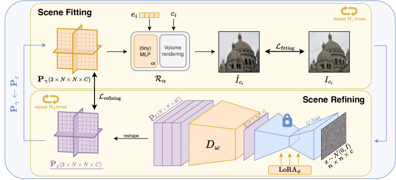
Figure 2: Scene learning procedure. The K-Planes $\mathbf{P}_{\gamma}$, the MLP with trainable parameters $\alpha$, and the appearance embeddings $e_{i}$ are learned during scene fitting. The LoRA parameters $\phi$ as well as the decoder $D_{w}$ are learned during scene refining. The pre-trained U-Net is frozen. Assets in violet and underlined are intermediate results. At each iteration, new planes $\mathbf{P}_{\varepsilon}$ are inferred and assigned to $\mathbf{P}_{\gamma}$, which are then corrected by scene fitting.

3 Method

To guide the optimization of scene representations with extrinsic signals, we learn a scene through two alternating stages, as illustrated in Figure 2. Scene fitting optimizes our K-Planes representation $\mathbf{P}_{\gamma}$ to reproduce the images in the training set, as traditionally done in neural rendering techniques. Scene refining finetunes a pre-trained network to this K-Planes representation, and then infers a new one $\mathbf{P}_{\varepsilon}$, which will subsequently be corrected by scene fitting. The main idea behind this is that we use our 3D implicit model $\mathbf{P}_{\gamma}$ for optimizing the scene to the available information in the training set and adhere to essential geometric constraints, and then project this scene representation on the set of scenes inferable by the pre-trained network, making it closer to natural images. In this section, we detail each stage and elucidate the intuition behind our method.

3.1 Scene Fitting

The goal at this stage is to fit a scene, adhering to pre-defined geometric constraints, from posed RGB images. To fit the scene, we adopt the K-Planes representation (Fridovich-Keil et al., 2023) (closely related to Tri-Planes (Chan et al., 2022) and HexPlanes (Cao & Johnson, 2023)). As such, this stage corresponds to following the optimization procedure of K-Planes representations as presented in (Fridovich-Keil et al., 2023), from which we adapt the code.

K-Planes are compact 3D model representations applicable to static scenes, “in-the-wild” scenes (scenes with varying appearances), and dynamic scenes. These models allow for fast training and rendering, while maintaining low-memory usage. K-Planes model a d-dimensional scene with $k=\binom{d}{2}$ planes, which represent the combinations of every pair of dimensions. This structure makes K-Planes compatible with a multitude of neural network architectures, and more particularly image-specialized network architectures. This enables K-Planes generation by minimally tweaking generative image architectures. For a static 3D scene, $k=3$ and the planes represent the $xy,xz,$ and $yz$ planes. These planes, each of size $N\times N\times C$, encapsulate features representing the density and view-dependent colors of the scene.

The K-Planes model $\mathbf{P}_{\gamma}$ is originally randomly initialized. The first goal of scene fitting is then to correct this random initialization to fit the training set. Note that the first iteration of scene fitting is especially particular, since it is starting with a randomly initialized scene, as opposed to a proposed scene, as we describe in Section 3.2.

To render the 3D scene from K-Planes, as done by Mildenhall et al. (2020) and Fridovich-Keil et al. (2023), we cast rays from the desired camera position through the coordinate space of the scene, on which we sample 3D points. We decode the corresponding RGB color for each 3D point $\mathbf{q}=(i,j,k)$ by normalizing it to $[0,N)$ and projecting it onto the $k=3$ planes, denoted as $\mathbf{P}_{\gamma}^{(xy)},\mathbf{P}_{\gamma}^{(xz)},\mathbf{P}_{\gamma}^{(yz)}$:

$$f^{(h)}(\mathbf{q})=\psi(\mathbf{P}_{\gamma}^{(h)},\pi^{(h)}(\mathbf{q}))~{},$$ (1)

where $h\in\mathbf{H}=\{xy,xz,yz\}$, $\pi^{(h)}(\mathbf{q})$ projects $\mathbf{q}$ onto $\mathbf{P}_{\gamma}^{(h)}$, and $\psi$ denotes bilinear interpolation on a regular 2D grid.

These features are then aggregated using the Hadamard product to produce a single feature vector of size $M$:

$$f(\mathbf{q})=\prod_{h\in\mathbf{H}}f^{(h)}(\mathbf{q})~{}.$$ (2)

To decode these features, we adopt the hybrid formulation of K-Planes (Fridovich-Keil et al., 2023). Two small Multi-Layer Perceptrons (MLPs), $g_{\sigma}$ and $g_{RGB}$, map the aggregated features as follows:

$$\begin{split}\sigma(\mathbf{q}),\hat{f}(\mathbf{q})&=g_{\sigma}(f(\mathbf{q}))~{},\\ c(\mathbf{q},\mathbf{d})&=g_{\mathrm{RGB}}(\hat{f}(\mathbf{q}),\gamma(\mathbf{d}))~{},\end{split}$$ (3)

where $\gamma(p)=(\sin(2^{0}\pi p),\cos(2^{0}\pi p),\ldots,\sin(2^{L-1}\pi p),$ $\cos(2^{L-1}\pi p))$ is the positional embedding of $p$. $g_{\sigma}$ maps the K-Planes features into density $\sigma$ and additional features $\hat{f}$. Subsequently, $g_{\mathrm{RGB}}$ maps $\hat{f}$ and the positionally-encoded view directions $\gamma(\mathbf{d})$ into view-dependent RGB colors. This enforces densities to be independent of view directions.

These decoded RGB colors are then used to render the final image thanks to ray marching and integrals from classical volume rendering (Kajiya & Herzen, 1984), that are practically estimated using quadrature:

$$\begin{split}\hat{C}(\mathbf{r})&=\sum_{i=1}^{N}T_{i}(1-\exp(-\sigma_{i}\delta_{i}))c_{i}~{},\\ T_{i}&=\exp\left(-\sum_{j=1}^{i-1}\sigma_{j}\delta_{j}\right)~{},\end{split}$$ (4)

where $\hat{C}(\mathbf{r})$ is the expected color, $T_{i}$ is the accumulated transmittance along the ray, and $\delta_{i}=t_{i+1}-t_{i}$ is the distance between adjacent samples. Proposal sampling is also employed similarly to Fridovich-Keil et al. (2023) to iteratively refine a small instance of K-Planes (using histogram loss (Barron et al., 2022)) that estimates densities along a ray. These density estimates are used to allocate more points in regions of higher densities.

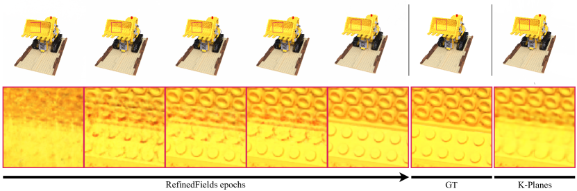
Figure 3: Synthetic toy example. Qualitative results on the Lego scene from the NeRF synthetic dataset (Mildenhall et al., 2020) showcasing the optimization progression on RefinedFields, and a comparison with the ground truth and K-Planes. The training set is constrained to 50% of its initial size for both RefinedFields and K-Planes. RefinedFields refines the K-Planes representation enabling the proper reconstruction of details in the scene. At the end of optimization, the Mean Squared Error (MSE) for RefinedFields is $3.46\times 10^{-4}$, while the one for K-Planes is $4.36\times 10^{-4}$.

3.2 Scene Refining

Given a fitted scene representation $\mathbf{P}_{\gamma}$, this stage consists of learning this fitted implicit representation and proposing a new refined representation. Formally, this stage consists of projecting our K-Planes $\mathbf{P}_{\gamma}$ on the set $\mathbb{Q}$ of K-Planes inferable by a low-rank fine-tuning of the pre-trained model:

$$\mathbf{P}_{\varepsilon}=\operatorname*{arg\,min}_{P\in\mathbb{Q}}~{}\lVert\mathbf{P}_{\gamma}-P\rVert~{}.$$ (5)

As K-Planes feature channels show similar structure to images (Appendix C), this projection pushes the K-Planes to be even more similar in structure to real images, more particularly to orthogonal projections of the scene on the planes. This leads to a better initialization for the K-Planes optimization, as proven by our experiments (Figures 3 and 2).

To provide scene refining with a rich prior, we employ a large-scale pre-trained latent diffusion model, as these networks exhibit great performances as priors for downstream tasks, and share similar properties to our planar representation, both in terms of shape and distribution (Appendix C). More particularly, we adopt Stable Diffusion (Rombach et al., 2022, SD) for its proven performances for downstream 3D (Liu et al., 2023) and 2D (Wang et al., 2023) tasks. Thus, we integrate the U-Net $\mathbf{SD}_{\phi}$ and the decoder $\mathbf{D}_{\omega}$ into our pipeline, and treat the K-Planes as $3C$-channel $N\times N$ images. We also replace the last layer of the decoder $\mathbf{D}_{\omega}$ with a randomly initialized convolutional layer (with no bias), to take into account the shape of the K-Planes. We then fine-tune the pre-trained model using the fitted K-Planes $\mathbf{P}_{\gamma}$, and infer refined K-Planes $\mathbf{P}_{\varepsilon}=\mathbf{D}_{w}(\mathbf{SD}_{\phi}(x))$ where $x\sim\mathcal{N}(0,I)$. Note that this is different from the multi-step generation process of diffusion model inference, as we only apply the inference at the last time-step of our diffusion model. This is key as our goal here is not to learn distributions over scenes and sample them for generation, but to adapt the pre-trained network and leverage the information already learned within its weights to infer K-Planes closest to representing the scene at hand.

Algorithm 1 Alternating training algorithm.

1:  Input: $N_{\mathrm{epochs}}$, $N_{1}$, $N_{2}$, $N$, $C$, $n$, $c$, $\mathcal{I}=\{I_{c_{i}},c_{i}\}$, $\mathcal{R}_{\alpha}$, $\mathbf{D}_{w}$, $\mathbf{SD}_{\phi}$, optimizer

2:  $x\leftarrow\text{standard-gaussian}(n,n,c)$

3:  $\mathbf{P}_{\gamma}\leftarrow\text{standard-gaussian}(N,N,3C)$

4:  for $N_{\mathrm{epochs}}$ steps do

5:     // scene fitting

6:     for $N_{1}$ steps do

7:        $\gamma,\alpha\leftarrow\text{optimizer.step}(\mathcal{L}_{\mathrm{fitting}}(\mathbf{P}_{\gamma},\mathcal{I}))$ 

8:     end for

9:     // scene refining

10:     for $N_{2}$ steps do

11:        $\mathbf{P}_{\varepsilon}\leftarrow\mathbf{D}_{w}(\mathbf{SD}_{\phi}(x))$

12:        $\omega,\phi\leftarrow\text{optimizer.step}(\mathcal{L}_{\mathrm{refining}}(\mathbf{P}_{\varepsilon},\mathbf{P}_{\gamma}))$

13:     end for

14:     $\mathbf{P}_{\gamma}\leftarrow\mathbf{P}_{\varepsilon}$ 

15:  end for

To achieve the fine-tuning of our pre-trained network, a significant challenge presents itself: due to the sheer size of Stable Diffusion, it would be exceptionally costly to fine-tune all of its trainable parameters. Moreover, as we only want to modulate priors embedded into the pre-trained network, we look for an alternative to doing full fine-tuning. To circumvent these constraints, we adopt Low-Rank Adaptation (Hu et al., 2022, LoRA), a simple yet effective parameter-efficient fine-tuning method that has proven great transfer capabilities across modalities and tasks (Fan et al., 2023; Lee et al., 2023; Zeng & Lee, 2023). LoRA’s relatively minimal design works directly over weight tensors, which means that it can be seamlessly applied to most model architectures. Furthermore, LoRA does not add any additional cost at inference, thanks to its structural re-parameterization design. To achieve this, Hu et al. (2022) inject trainable low-rank decomposition matrices into each layer of a frozen pre-trained model. Let $\mathbf{W}_{0}$, $\mathbf{b}_{0}$ be the frozen pre-trained weights and biases, and $x$ be the input. Fine-tuning a frozen linear layer $f(x)=\mathbf{W}_{0}x+\mathbf{b}_{0}$ comes down to learning the low-rank decomposition weights $\Delta\mathbf{W}=\mathbf{B}\mathbf{A}$:

$$f(x)=(\mathbf{W}_{0}+\Delta\mathbf{W})x+\mathbf{b}_{0}$$ (6)

where $\mathbf{W}_{0},\Delta\mathbf{W}\in\mathbb{R}^{d\times k}$; $\mathbf{B}\in\mathbb{R}^{d\times r}$; $\mathbf{A}\in\mathbb{R}^{r\times k}$; and the rank $r\ll\min(d,k)$.

Thus, to implement scene refining, we fine-tune the LoRA parameters $\phi$ modulating the pre-trained U-Net, as well as the decoder’s parameters $\omega$, on the fitted scene $\mathbf{P}_{\gamma}$. Subsequently, we query the U-Net with Gaussian noise $x$, decode its intermediary output latent $z$ with $\mathbf{D}_{\omega}$, and infer $\mathbf{p}_{\varepsilon}$ that is reshaped into a new refined scene $\mathbf{P}_{\varepsilon}$. Finally, $\mathbf{P}_{\varepsilon}$ is proposed to scene fitting as an improved initialization to be optimized. For an in-depth inspection of the feature planes, we highly encourage the reader to refer to Appendix C.

3.3 Training

We define an alternating training procedure rotating between scene fitting and scene refining, as described above, and as illustrated in Figure 2.

For scene fitting, we train the K-Planes model as proposed by Fridovich-Keil et al. (2023). We use spatial total variation regularization to encourage smooth gradients. This is applied over all the spatial dimensions of each plane in the representation:

$$\begin{multlined}\mathcal{L}_{\mathrm{TV}}(\mathbf{P})=\frac{1}{|C|N^{2}}\sum_{c,i,j}(\lVert\mathbf{P}_{c}^{i,j}-\mathbf{P}_{c}^{i-1,j}\rVert_{2}^{2}\\ +\lVert\mathbf{P}_{c}^{i,j}-\mathbf{P}_{c}^{i,j-1}\rVert_{2}^{2})~{}.\end{multlined}\mathcal{L}_{\mathrm{TV}}(\mathbf{P})=\frac{1}{|C|N^{2}}\sum_{c,i,j}(\lVert\mathbf{P}_{c}^{i,j}-\mathbf{P}_{c}^{i-1,j}\rVert_{2}^{2}\\ +\lVert\mathbf{P}_{c}^{i,j}-\mathbf{P}_{c}^{i,j-1}\rVert_{2}^{2})~{}.$$ (7)

For scenes with varying lighting conditions (e.g. in-the-wild scenes as in the Phototourism dataset (Jin et al., 2020)), an $M$-dimensional appearance vector $e_{i}$ is additionally optimized for each image. This vector is then passed as input to the MLP color decoder $g_{RGB}$ at the rendering step $\mathcal{R}_{\alpha}$. Hence, the training objective for scene fitting is written as:

$$\min_{\alpha,\gamma}\mathcal{L}_{\mathrm{fitting}}\triangleq\lVert\mathcal{R}_{\alpha}(\mathbf{P}_{\gamma},\mathbf{C})-I_{\mathbf{C}}\rVert_{2}^{2}+\lambda_{\mathrm{TV}}\mathcal{L}_{\mathrm{TV}}(\mathbf{P}_{\gamma})~{},$$ (8)

where $\mathcal{R}_{\alpha}$ represents the K-Planes rendering procedure (i.e. ray marching, feature decoding via a small MLP with trainable parameters $\alpha$, and volume rendering), $\mathbf{P}_{\gamma}$ are the K-Planes with trainable parameters $\gamma$ and $I_{\mathbf{C}}$ is a ground truth RGB image with camera position $\mathbf{C}$.

As for the scene refining phase, we optimize the decoder parameters $w$ as well as the LoRA parameters $\phi$, modulating the frozen U-Net weights, on the fitted scene $\mathbf{P}_{\gamma}$. Thus, the fine-tuning objective for scene refining is written as:

$$\min_{w,\phi}\mathcal{L}_{\mathrm{refining}}\triangleq\lVert\mathbf{D}_{w}(\mathbf{SD}_{\phi}(x))-\mathbf{P}_{\gamma}\rVert_{2}^{2}~{},$$ (9)

where $x\sim\mathcal{N}(0,I)$ is fixed during scene refining, $\mathbf{SD}_{\phi}$ is the frozen Stable Diffusion model modulated by LoRA with trainable parameters $\phi$, and $\mathbf{D}_{w}$ is the latent K-Planes decoder. After this optimization, $\mathbf{P}_{\gamma}$ is reassigned as $\mathbf{D}_{w}(\mathbf{SD}_{\phi}(x))$ and passed to scene fitting. Note that, thanks to the alternating nature of our training and the absence of bias in the decoder’s convolutional layers, this optimization does not reach full convergence. This is key because over-fitting the generative model to generate exactly $\mathbf{P}_{\gamma}$ leads to resuming scene fitting from exactly the same point.

At the end of the alternating training procedure, we save the refined and corrected representation $\mathbf{P}_{\gamma}$ for rendering and testing. We refer the reader to Algorithm 1 for an overview of our training procedure.

4 Experiments

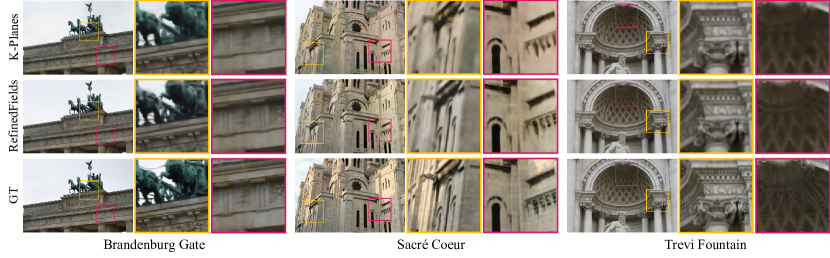
Figure 4: Qualitative results. Results on three scenes from Phototourism (Jin et al., 2020). Our method refines K-Planes and leads to richer and finer details in scene renderings.

Table 2: Quantitative results. Results on three real-world datasets from Phototourism (Jin et al., 2020). The bold and underlined entries respectively indicate the best and second-best results. Our method demonstrates state-of-the-art performance on the task of NVS-W.

Brandenburg Gate Sacré Coeur Trevi Fountain PSNR ($\uparrow$) SSIM ($\uparrow$) PSNR ($\uparrow$) SSIM ($\uparrow$) PSNR ($\uparrow$) SSIM ($\uparrow$) NeRF (Mildenhall et al., 2020) 18.90 0.8159 15.60 0.7155 16.14 0.6007 NeRF-W (Martin-Brualla et al., 2021) 24.17 0.8905 19.20 0.8076 18.97 0.6984 Ha-NeRF (Chen et al., 2022b) 24.04 0.8773 20.02 0.8012 20.18 0.6908 CR-NeRF (Yang et al., 2023) 26.53 0.9003 22.07 0.8233 21.48 0.7117 K-Planes (Fridovich-Keil et al., 2023) 25.49 0.8785 20.61 0.7735 22.67 0.7139 K-Planes-SS (Fridovich-Keil et al., 2023) 24.48 0.8629 19.86 0.7419 21.30 0.6627 RefinedFields-noFinetuning (ours) 25.39 0.8834 21.41 0.8059 22.54 0.7324 RefinedFields-noPrior (ours) 25.42 0.8822 21.17 0.7978 22.16 0.7251 RefinedFields (ours) 26.64 0.8869 22.26 0.8176 23.42 0.7379

We start by assessing RefinedFields via an experiment on a synthetic example. We then evaluate RefinedFields on real-world Phototourism (Jin et al., 2020) scenes, where we showcase the improvements our method exhibits relative to our K-Planes base representation, and compare with other recent methods tackling novel view synthesis in-the-wild (Martin-Brualla et al., 2021; Chen et al., 2022b; Yang et al., 2023). Quantitative results can be found in Table 2, where we report for each experiment the Peak Signal-to-Noise Ratio (PSNR) for pixel-level similarity and the Structural Similarity Index Measure (SSIM) for structural-level similarity. RefinedFields demonstrates superior performance compared to K-Planes as well as recent methods tackling novel view synthesis in-the-wild. For a further look, experimental details including hyperparameters and more dataset details can be found in Appendix B. Quantitative results on addtional synthetic scenes can be found in Appendix D. Additional real-world qualitative results on Phototourism (Jin et al., 2020) are also available in Appendix D.

4.1 Datasets

We evaluate our method similarly to prior work (Martin-Brualla et al., 2021; Chen et al., 2022b; Fridovich-Keil et al., 2023) in novel view synthesis in-the-wild, by adopting the same three scenes of cultural monuments from the Phototourism dataset (Jin et al., 2020): Brandenburg Gate, Sacré Coeur, and Trevi Fountain. Additional dataset details can be found in Appendix B.

4.2 Implementation Details

For a fair comparison, we take similar experimental settings in scene fitting to Fridovich-Keil et al. (2023). However, due to the nature of our scene refining pipeline, we limit the implementation in our case to a single-scale K-Planes of $512\times 512$ resolution, in contrast to the multi-scale approach taken by Fridovich-Keil et al. (2023) where $N\in\{64,128,256,512\}$. The number of channels in each plane remains the same ($C=32$). Also note that throughout all the experiments, we consider the hybrid implementation of K-Planes, where plane features are decoded into colors and densities by a small MLP. As for the scene refining pipeline, we apply no modification to the U-Net in Stable Diffusion. Yet, we replace the last layer of the decoder $D_{\omega}$ with a new convolutional layer (without bias) to account for the shape of the K-Planes. Hence, the dimensions we work with in scene refining (Figure 2) are: $N=512$, $C=32$, $n=64$, and $c=4$. For an in-depth look at our hyperparameter settings, we refer the reader to Appendix B.

4.3 Evaluations

Baselines.

We compare our results against NeRF-W (Martin-Brualla et al., 2021) (results from the public implementation (Aoi, 2022)), Ha-NeRF (Chen et al., 2022b), CR-NeRF (Yang et al., 2023) and K-Planes (Fridovich-Keil et al., 2023). Note that, to assess the added value of our refining pipeline with respect to our base representation (Section 4.2), we also include a single-scale ablation of K-Planes with $N=512$ (dubbed K-Planes-SS).

Comparisons.

We start by testing our method against K-Planes on a toy example consisting of the Lego scene from the NeRF synthetic dataset. Here, we train both methods on half of the training set. As illustrated in Figure 3 our method refines K-Planes and exhibits better quantitative and qualitative results thanks to our scene refining pipeline.

We then apply our method on in-the-wild scenes. In this case, RefinedFields outperforms not only K-Planes-SS but also K-Planes and previous state-of-the-art methods in NVS-W (Table 2). This particularly highlights the value of scene refining. Our method demonstrates a significant PSNR margin ranging between 1.15 and 2.6 for Brandenburg Gate, 1.65 and 3.06 for Sacré Coeur, and 0.75 and 4.45 for Trevi Fountain as compared to previous works in novel view synthesis in-the-wild (excluding NeRF and CR-NeRF). We consider CR-NeRF (Yang et al., 2023) to be concurrent to our work. Still, our method shows marginal improvements compared to CR-NeRF on Brandenburg Gate and Sacré Coeur, and a PSNR increase of 1.94 on the Trevi Fountain scene. Figures 1 and 4 show qualitative comparisons of RefinedFields with K-Planes, showing the visual improvements brought by our refining pipeline, which brings finer details to monuments in the Phototourism scenes. Further qualitative results can be found in Appendix D.

4.4 Ablations

To justify our choices and explore further, we compare our in-the-wild results (Table 2) to results from two main ablations of our method. RefinedFields-noFinetuning is a variation of our method without LoRA fine-tuning. Here, we consider the same exact pipeline (frozen U-Net, same decoder configuration), except that we don’t modulate the weights of the frozen U-Net with LoRA. This means that the prior is kept intact and no fine-tuning is done. This is to assess the role that LoRA finetuning of the pre-trained prior plays in our pipeline. RefinedFields-noPrior ablates the prior of Stable Diffusion by randomly re-initializing all U-Net weights while leaving all other elements of the scene-refining pipeline intact. This ablation is done to evaluate the importance of the prior, and to verify that the observed refinements are not entirely resulting from alternate training. Note that ablating the entire scene refining pipeline leads back to the K-Planes-SS setting. As illustrated in Table 2, we consistently obtain worse results during the ablation study as compared to our full model, thus demonstrating the value of the pre-trained prior and of LoRA finetuning. This proves the importance of extending scene learning beyond closed-world settings, as our optimization conditioning comes from a large image prior that a reasonably sized training set cannot fully capture, especially in-the-wild.

4.5 Training Time Analysis

As presented, RefinedFields utilizes an alternating training procedure and a pre-trained prior to refine scene representations, leading to richer details in rendered images. While our method demonstrates interesting results, this however comes with a training time increase as compared to our base representation, as our alternating training leads to the repeated fine-tuning of both scene fitting and scene refining pipelines. In addition, in order for this training to converge well, we apply a relatively small learning rate ($10^{-4}$) to the LoRA parameters. While we leave training time optimizations for future work, our method still requires significantly less training time compared to its concurrent works in novel view synthesis in-the-wild (Table 3).

Table 3: Training times. Comparison of training time among methods tackling novel view synthesis in-the-wild. Timings are based on a single NVIDIA V100 GPU. Our method demonstrates state-of-the-art performance in about a third of the training time needed in its concurrent work.

	Training Time ($\downarrow$)
NeRF-W (Martin-Brualla et al., 2021)	400 hrs
Ha-NeRF (Chen et al., 2022b)	452 hrs
CR-NeRF (Yang et al., 2023)	420 hrs
K-Planes (Fridovich-Keil et al., 2023)	50 mins
RefinedFields (ours)	150 hrs

5 Conclusion

In this paper, we introduce RefinedFields, a method that refines K-Planes representations by incorporating a pre-trained prior and alternate training . Extensive experiments show that RefinedFields exhibits notable improvements on real-world monument details. In concluding this study, several avenues of future work emerge as we consider this work to be a first stepping-stone in conditioning closed-world in-the-wild scene representations with extrinsic signals. This includes the exploration of approaches to achieve this conditioning other than optimization guidance, the application of scene refining on other representations, and the extension of appearance modeling beyond learnable embeddings.

Impact Statement

This paper presents work that enhances the construction of high-quality neural representations. As such, the risks associated with our work parallel those of other neural rendering papers. This includes but is not limited to privacy and security concerns, as our method is trained on a dataset of publicly captured images, where privacy-sensitive information (e.g. human faces, license plate numbers) could be present. Hence, similarly to other neural rendering approaches, there is a risk that such data could end up in the trained model if the employed datasets are not properly filtered before use. Furthermore, as our work utilizes Stable Diffusion as prior, it inherits any problematic biases and limitations this model may have (Carlini et al., 2023; Luccioni et al., 2023).

Appendix A Related Work Overview

Due to space constraints, this section presents the referenced version of Table 1 in the main paper.

Table 4: Related work overview. RefinedFields leverages unconstrained tourist photo collections (Jin et al., 2020) and a pre-trained prior (Rombach et al., 2022) to refine K-Planes, our underlying scene representation, in order to achieve state-of-the-art performance in in-the-wild scene modeling.

	No 3D supervision	Pre-trained prior	Geometric consistency	In-the-wild scene modeling	Underlying representation	Task
NeRF (Mildenhall et al., 2020)	✓	✗	✓	✗	NeRF	NVS
K-Planes (Fridovich-Keil et al., 2023)	✓	✗	✓	✓	K-Planes
NFD (Shue et al., 2023)	✗	✗	✓	✗	Tri-Planes	OG
3DGen (Gupta et al., 2023)	✗	✗	✓	✗	Tri-Planes
Latent-NeRF (Metzer et al., 2023)	✓	✓	✓	✗	NeRF
DreamFusion (Poole et al., 2023)	✓	✓	✓	✗	NeRF
PixelNeRF (Yu et al., 2021)	✓	✓	✓	✗	NeRF	NVS
NeRDi (Deng et al., 2023)	✓	✓	✓	✗	NeRF
RealFusion (Melas-Kyriazi et al., 2023)	✓	✓	✓	✗	NeRF
DiffusioNeRF (Wynn & Turmukhambetov, 2023)	✓	✗	✓	✗	NeRF
NerfDiff (Gu et al., 2023)	✗	✓	✓	✗	Tri-Planes
3DiM (Watson et al., 2023)	✗	✗	✓	✗	—
Zero-1-to-3 (Liu et al., 2023)	✗	✓	✗	✗	—
NeRF-W (Martin-Brualla et al., 2021)	✓	✗	✓	✓	NeRF	NVS-W
Ha-NeRF (Chen et al., 2022b)	✓	✗	✓	✓	NeRF
CR-NeRF (Yang et al., 2023)	✓	✗	✓	✓	NeRF
RefinedFields (ours)	✓	✓	✓	✓	K-Planes

Appendix B Experimental Details

B.1 Datasets

Synthetic dataset.

For synthetic renderings, we adopt the Real Synthetic $\mathit{360^{\circ}}$ dataset from NeRF (Mildenhall et al., 2020). This dataset consists of eight path-traced scenes containing objects exhibiting complicated geometry and realistic non-Lambertian materials. Each image is coupled with its corresponding camera parameters. Consistently with prior work, 100 images are used for training each scene and 200 images are used for testing. All images are at $800\times 800$ pixels.

In-the-wild dataset.

For in-the-wild renderings, we adopt the Phototourism dataset (Jin et al., 2020) which is commonly used for in-the-wild tasks. This dataset consists of multitudes of images of touristic landmarks gathered from the internet. Thus, these images are naturally plagued by visual discrepancies, notably illumination variation and transient occluders. Camera parameters are estimated using COLMAP (Schönberger & Frahm, 2016). All images are normalized to [0,1]. We adopt three scenes from Phototurism: Brandenburg Gate (1363 images), Sacré Coeur (1179 images), and Trevi Fountain (3191 images). Testing is done on a standard set that is free of transient occluders.

B.2 Frameworks

We make use of multiple frameworks to implement our method. Our Python source code (tested on version 3.7.16), based on PyTorch (Paszke et al., 2019) (tested on version 1.13.1) and CUDA (tested on version 11.6), will be publicly available as open source. We also utilize Diffusers (von Platen et al., 2022) and Stable Diffusion (tested on version 1-5, main revision). K-Planes also adopt the tinycudann framework (Müller, 2021). We run all experiments on a single NVIDIA V100 GPU.

B.3 Hyperparameters

A summary of our hyperparameters for synthetic as well as in-the-wild scenes can be found in Table 6.

Appendix C Feature Planes Inspection

In this section, we present a visual inspection of K-Planes feature planes within different contexts. Figures 5, 6 and 7 each correspond to one out of the three orthogonal planes. Each element in Figures 5, 6 and 7 presents a single feature plane, picked randomly from the $C$ feature planes. Figures 5a, 6a and 7a represent the state of the planes at an intermediate stage of the RefinedFields optimization process. Figures 5b, 6b and 7b represent the state of the planes at the end of the RefinedFields optimization. Figures 5c, 6c and 7c represent the planes at the end of the K-Planes-SS optimization (no refining is done in this case).

Two noteworthy observations emerge. First, as seen in Figures 5, 6 and 7, K-Planes feature planes are very similar in structure to real images. In fact, these feature planes depict orthogonal projections of the scene onto the planes. These findings are especially compelling, as they justify the appropriate choice of Stable Diffusion as the pre-trained prior for the refining stage, and provide insight onto the quantitative and qualitative results showcased by our method. Second, a comparison between columns [5b, 6b and 7b] and [5c, 6c and 7c] highlights the impact scene refining has on the feature planes themselves, as planes 5b, 6b and 7b exhibit details that are more similar in structure to the scene, and that are sharper than planes 5c, 6c and 7c.

Appendix D Supplementary Results

Quantitative results.

We reproduce the results on K-Planes and K-Planes-SS. In-the-wild results on NeRF-W come from a public implementation of the paper (Aoi, 2022) and are extracted from the K-Planes paper. Ha-NeRF and CR-NeRF results are extracted from the recent CR-NeRF paper. Remaining results in Tables 5 and 2 are extracted from their corresponding papers.

Qualitative results.

We present below additional qualitative results for in-the-wild scenes (Figures 8, 9 and 10) and synthetic renderings Figures 11 and 12. Please refer to our project page for animations of our renderings.

(a)

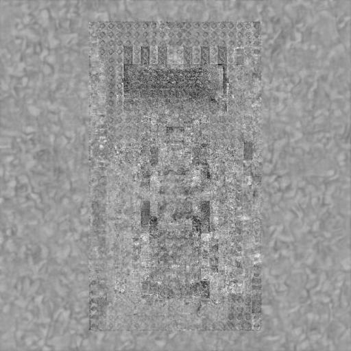
(b)

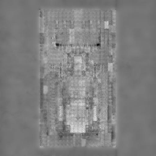
(c)

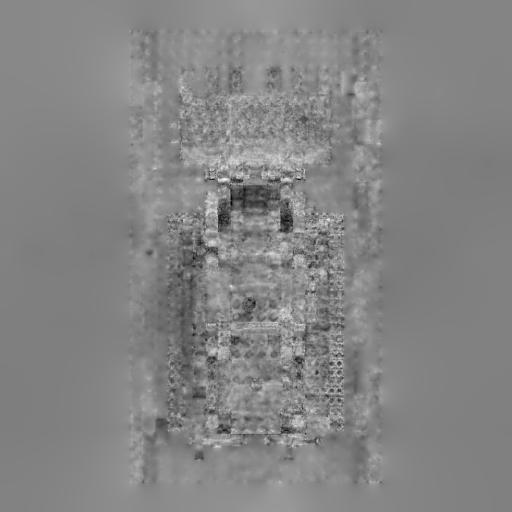
(d)

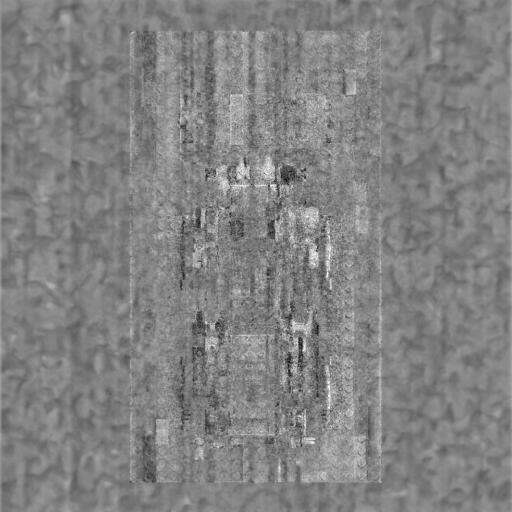
(e)

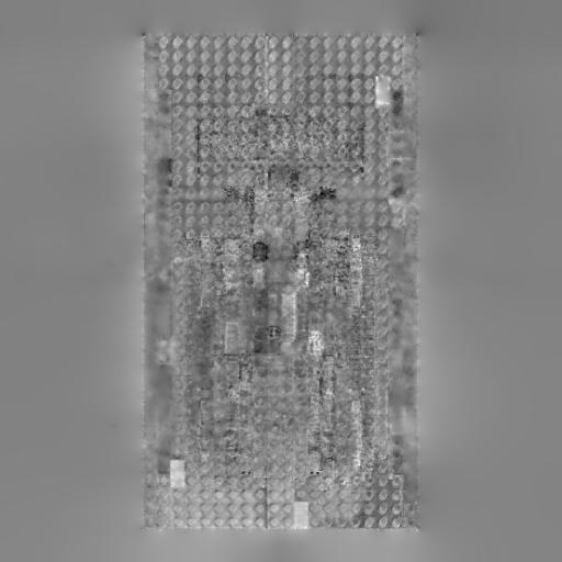
(f)

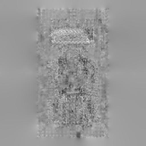
(g)

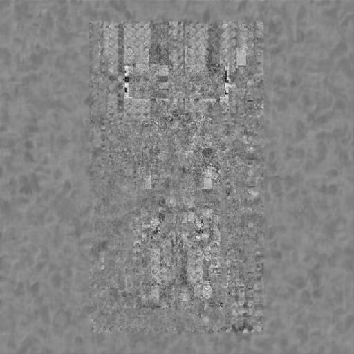
(a) RefinedFields (In-Process)

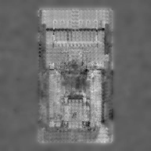
(b) RefinedFields (Final)

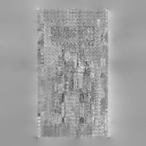
(c) K-Planes

Figure 5: Feature planes inspection. Visualization of the $(xy)$ K-Planes feature planes during the RefinedFields optimization process (5a), at the end of the RefinedFields optimization (5b), and a comparison with vanilla K-Planes-SS (5c). Feature planes within the $(xy)$ K-Planes are picked randomly.

(a)

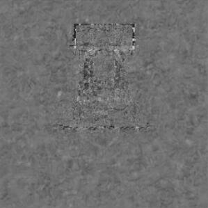
(b)

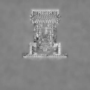
(c)

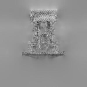
(d)

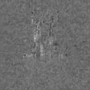
(e)

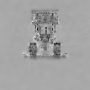
(f)

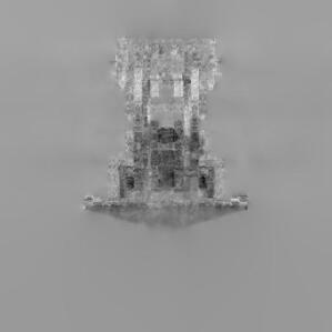
(g)

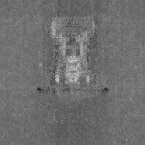
(a) RefinedFields (In-Process)

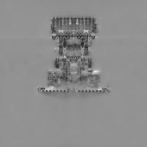
(b) RefinedFields (Final)

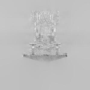
(c) K-Planes

Figure 6: Feature planes inspection. Visualization of the $(xz)$ K-Planes feature planes during the RefinedFields optimization process (6a), at the end of the RefinedFields optimization (6b), and a comparison with vanilla K-Planes-SS (6c). Feature planes within the $(xz)$ K-Planes are picked randomly.

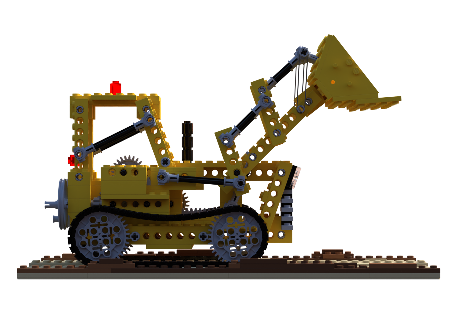
(a)

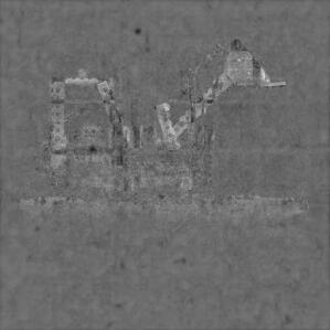
(b)

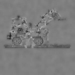
(c)

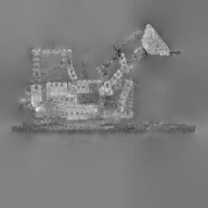
(d)

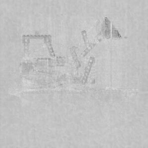
(e)

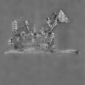
(f)

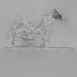
(g)

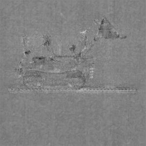
(a) RefinedFields (In-Process)

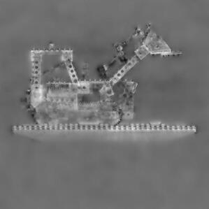
(b) RefinedFields (Final)

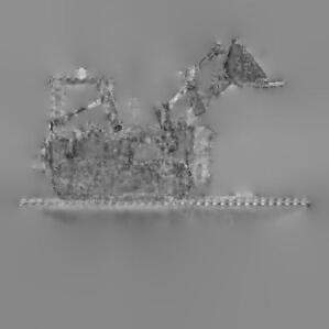
(c) K-Planes

Figure 7: Feature planes inspection. Visualization of the $(yz)$ K-Planes feature planes during the RefinedFields optimization process (7a), at the end of the RefinedFields optimization (7b), and a comparison with vanilla K-Planes-SS (7c). Feature planes within the $(yz)$ K-Planes are picked randomly.

Table 5: Quantitative results. Results on static synthetic scenes (Mildenhall et al., 2020). The bold and underlined entries respectively indicate the best and second-best results. Dashes denote values that were not reported in prior work. Our method outperforms K-Planes, our main baseline, on the task of novel view synthesis for synthetic scenes.

	PSNR ($\uparrow$)
	Chair	Drums	Ficus	Hotdog	Lego	Materials	Mic	Ship		Mean
NeRF (Mildenhall et al., 2020)	33.00	25.01	30.13	36.18	32.54	29.62	32.91	28.65		31.00
TensoRF (Chen et al., 2022a)	35.76	26.01	33.99	37.41	36.46	30.12	34.61	30.77		33.14
Plenoxels (Fridovich-Keil et al., 2022)	33.98	25.35	31.83	36.43	34.10	29.14	33.26	29.62		31.71
INGP (Müller et al., 2022)	35.00	26.02	33.51	37.40	36.39	29.78	36.22	31.10		33.18
K-Planes (Fridovich-Keil et al., 2023)	34.98	25.68	31.44	36.75	35.81	29.48	34.10	30.76		32.37
K-Planes-SS (Fridovich-Keil et al., 2023)	33.61	25.27	30.92	35.88	35.09	28.83	33.01	30.04		31.58
RefinedFields (ours)	35.77	25.94	32.45	37.08	36.47	29.39	34.77	31.41		32.91

	SSIM ($\uparrow$)
	Chair	Drums	Ficus	Hotdog	Lego	Materials	Mic	Ship		Mean
NeRF (Mildenhall et al., 2020)	0.967	0.925	0.964	0.974	0.961	0.949	0.980	0.856		0.947
TensoRF (Chen et al., 2022a)	0.985	0.937	0.982	0.982	0.983	0.952	0.988	0.895		0.963
Plenoxels (Fridovich-Keil et al., 2022)	0.977	0.933	0.976	0.980	0.975	0.949	0.985	0.890		0.958
INGP (Müller et al., 2022)	—	—	—	—	—	—	—	—		—
K-Planes (Fridovich-Keil et al., 2023)	0.983	0.938	0.975	0.982	0.982	0.950	0.988	0.897		0.962
K-Planes-SS (Fridovich-Keil et al., 2023)	0.974	0.932	0.971	0.977	0.978	0.943	0.983	0.887		0.956
RefinedFields (ours)	0.985	0.937	0.980	0.981	0.984	0.945	0.989	0.903		0.963

Table 6: Hyperparameters. A summary of the hyperparameters used to train our model. Appearance optimizations only apply for in-the-wild training.
^∗Note that this parameter is taken differently from Fridovich-Keil et al. (2023), as we only work with single-scale planes. We consider the highest plane resolution from the multi-scale approach taken by Fridovich-Keil et al. (2023).

Hyperparameter	Value
Epochs ($N_{\mathrm{epochs}}$)	200 (synthetic) 20 (Sacré Coeur) 20 (Brandenburg Gate) 10 (Trevi Fountain)
Epochs K-Planes ($N_{1}$)	1
Epochs LoRA ($N_{2}$)	3000
Batch size	4096
Optimizer	Adam
Scheduler	Warmup Cosine
K-Planes Learning Rate	0.01
LoRA Learning rate	0.0001
SD latent resolution	64
SD channel dimension	4
SD prompt	“ ”
Number of planes	3
K-Planes resolution∗	512
K-Planes channel dimension	32
Epochs Appearance Optimization	10
Appearance embeddings dimension	32
Appearance learning rate	0.1 (Sacré Coeur) 0.1 (Trevi Fountain) 0.001 (Brandenburg Gate)
Appearance batch size	512

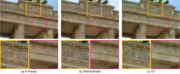
Figure 8: Qualitative results. Results on the Brandenburg Gate scene from Phototourism (Jin et al., 2020).

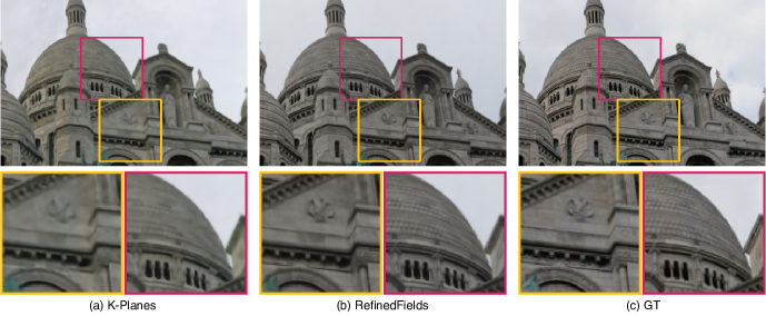
Figure 9: Qualitative results. Results on the Sacré Coeur scene from Phototourism (Jin et al., 2020).

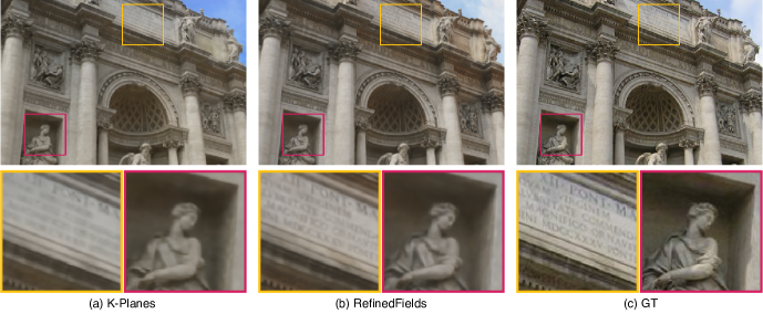
Figure 10: Qualitative results. Results on the Trevi Fountain scene from Phototourism (Jin et al., 2020).

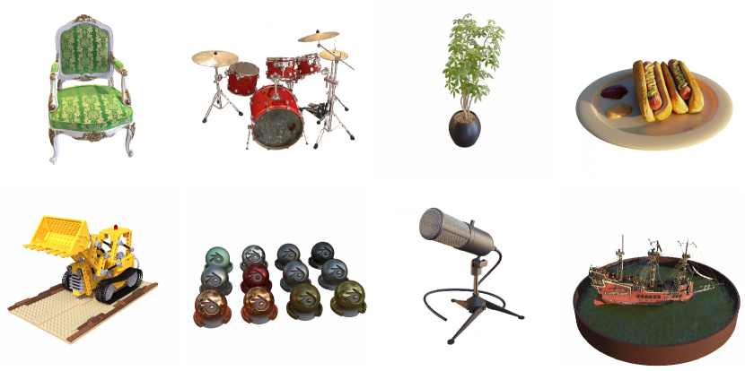
Figure 11: Qualitative results. RefinedFields results on the NeRF Synthetic scenes.

Figure 12: Ground Truth Renderings. Ground truth images from the NeRF Synthetic dataset.

References

- Aoi (2022) Aoi, A. nerf_pl. https://github.com/kwea123/nerf_pl/tree/nerfw, 2022. Accessed: 2023-10-25.
- Barron et al. (2022) Barron, J. T., Mildenhall, B., Verbin, D., Srinivasan, P. P., and Hedman, P. Mip-NeRF 360: Unbounded Anti-Aliased Neural Radiance Fields. In Proceedings of the IEEE/CVF Conference on Computer Vision and Pattern Recognition (CVPR), pp. 5470–5479, June 2022.
- Cao & Johnson (2023) Cao, A. and Johnson, J. HexPlane: A Fast Representation for Dynamic Scenes. In Proceedings of the IEEE/CVF Conference on Computer Vision and Pattern Recognition (CVPR), pp. 130–141, June 2023.
- Carlini et al. (2023) Carlini, N., Hayes, J., Nasr, M., Jagielski, M., Sehwag, V., Tramer, F., Balle, B., Ippolito, D., and Wallace, E. Extracting training data from diffusion models. In 32nd USENIX Security Symposium (USENIX Security 23), pp. 5253–5270, 2023.
- Chan et al. (2022) Chan, E. R., Lin, C. Z., Chan, M. A., Nagano, K., Pan, B., De Mello, S., Gallo, O., Guibas, L. J., Tremblay, J., Khamis, S., Karras, T., and Wetzstein, G. Efficient Geometry-Aware 3D Generative Adversarial Networks. In Proceedings of the IEEE/CVF Conference on Computer Vision and Pattern Recognition (CVPR), pp. 16123–16133, June 2022.
- Chen et al. (2022a) Chen, A., Xu, Z., Geiger, A., Yu, J., and Su, H. TensoRF: Tensorial Radiance Fields. In European Conference on Computer Vision (ECCV), 2022a.
- Chen et al. (2022b) Chen, X., Zhang, Q., Li, X., Chen, Y., Feng, Y., Wang, X., and Wang, J. Hallucinated Neural Radiance Fields in the Wild. In Proceedings of the IEEE/CVF Conference on Computer Vision and Pattern Recognition (CVPR), pp. 12943–12952, June 2022b.
- Cohen & Szeliski (2014) Cohen, M. F. and Szeliski, R. Lumigraph, pp. 462–467. Springer US, Boston, MA, 2014. ISBN 978-0-387-31439-6. doi: 10.1007/978-0-387-31439-6_8.
- Deng et al. (2023) Deng, C., Jiang, C. M., Qi, C. R., Yan, X., Zhou, Y., Guibas, L., and Anguelov, D. Nerdi: Single-view nerf synthesis with language-guided diffusion as general image priors. In Proceedings of the IEEE/CVF Conference on Computer Vision and Pattern Recognition (CVPR), pp. 20637–20647, June 2023.
- Fan et al. (2023) Fan, Y., Watkins, O., Du, Y., Liu, H., Ryu, M., Boutilier, C., Abbeel, P., Ghavamzadeh, M., Lee, K., and Lee, K. Dpok: Reinforcement learning for fine-tuning text-to-image diffusion models. arXiv preprint arXiv:2305.16381, 2023.
- Fridovich-Keil et al. (2022) Fridovich-Keil, S., Yu, A., Tancik, M., Chen, Q., Recht, B., and Kanazawa, A. Plenoxels: Radiance Fields Without Neural Networks. In Proceedings of the IEEE/CVF Conference on Computer Vision and Pattern Recognition (CVPR), pp. 5501–5510, June 2022.
- Fridovich-Keil et al. (2023) Fridovich-Keil, S., Meanti, G., Warburg, F. R., Recht, B., and Kanazawa, A. K-Planes: Explicit Radiance Fields in Space, Time, and Appearance. In Proceedings of the IEEE/CVF Conference on Computer Vision and Pattern Recognition (CVPR), pp. 12479–12488, June 2023.
- Genova et al. (2020) Genova, K., Cole, F., Sud, A., Sarna, A., and Funkhouser, T. Local Deep Implicit Functions for 3D Shape. In IEEE/CVF Conference on Computer Vision and Pattern Recognition (CVPR), June 2020.
- Gimini (2016) Gimini, G. Velocipedia. https://www.gianlucagimini.it/portfolio-item/velocipedia/, 2016. Accessed: 2023-10-25.
- Graikos et al. (2022) Graikos, A., Malkin, N., Jojic, N., and Samaras, D. Diffusion Models as Plug-and-Play Priors. In Koyejo, S., Mohamed, S., Agarwal, A., Belgrave, D., Cho, K., and Oh, A. (eds.), Advances in Neural Information Processing Systems, volume 35, pp. 14715–14728. Curran Associates, Inc., 2022.
- Gu et al. (2023) Gu, J., Trevithick, A., Lin, K.-E., Susskind, J., Theobalt, C., Liu, L., and Ramamoorthi, R. NerfDiff: Single-image View Synthesis with NeRF-guided Distillation from 3D-aware Diffusion. In International Conference on Machine Learning, 2023.
- Gupta et al. (2023) Gupta, A., Xiong, W., Nie, Y., Jones, I., and Oğuz, B. 3dgen: Triplane latent diffusion for textured mesh generation. arXiv preprint arXiv:2303.05371, 2023.
- Hartley & Zisserman (2004) Hartley, R. and Zisserman, A. Multiple View Geometry in Computer Vision. Cambridge University Press, 2 edition, 2004. doi: 10.1017/CBO9780511811685.
- Ho et al. (2020) Ho, J., Jain, A., and Abbeel, P. Denoising Diffusion Probabilistic Models. In Larochelle, H., Ranzato, M., Hadsell, R., Balcan, M., and Lin, H. (eds.), Advances in Neural Information Processing Systems, volume 33, pp. 6840–6851. Curran Associates, Inc., 2020.
- Hu et al. (2022) Hu, E. J., Shen, Y., Wallis, P., Allen-Zhu, Z., Li, Y., Wang, S., Wang, L., and Chen, W. LoRA: Low-Rank Adaptation of Large Language Models. In International Conference on Learning Representations, 2022.
- Jain et al. (2021) Jain, A., Tancik, M., and Abbeel, P. Putting nerf on a diet: Semantically consistent few-shot view synthesis. In Proceedings of the IEEE/CVF International Conference on Computer Vision (ICCV), pp. 5885–5894, October 2021.
- Jin et al. (2020) Jin, Y., Mishkin, D., Mishchuk, A., Matas, J., Fua, P., Yi, K. M., and Trulls, E. Image Matching Across Wide Baselines: From Paper to Practice. International Journal of Computer Vision, 129(2):517–547, oct 2020. doi: 10.1007/s11263-020-01385-0.
- Kajiya & Herzen (1984) Kajiya, J. T. and Herzen, B. V. Ray tracing volume densities. Proceedings of the 11th annual conference on Computer graphics and interactive techniques, 1984.
- Kerbl et al. (2023) Kerbl, B., Kopanas, G., Leimkühler, T., and Drettakis, G. 3D Gaussian Splatting for Real-Time Radiance Field Rendering. ACM Transactions on Graphics, 42(4), July 2023.
- Lee et al. (2023) Lee, A. N., Hunter, C. J., and Ruiz, N. Platypus: Quick, cheap, and powerful refinement of llms. arXiv preprint arXiv:2308.07317, 2023.
- Liu et al. (2023) Liu, R., Wu, R., Van Hoorick, B., Tokmakov, P., Zakharov, S., and Vondrick, C. Zero-1-to-3: Zero-shot One Image to 3D Object. In Proceedings of the IEEE/CVF International Conference on Computer Vision (ICCV), pp. 9298–9309, October 2023.
- Luccioni et al. (2023) Luccioni, S., Akiki, C., Mitchell, M., and Jernite, Y. Stable bias: Evaluating societal representations in diffusion models. In Thirty-seventh Conference on Neural Information Processing Systems Datasets and Benchmarks Track, 2023.
- Martin-Brualla et al. (2021) Martin-Brualla, R., Radwan, N., Sajjadi, M. S. M., Barron, J. T., Dosovitskiy, A., and Duckworth, D. NeRF in the Wild: Neural Radiance Fields for Unconstrained Photo Collections. In Proceedings of the IEEE/CVF Conference on Computer Vision and Pattern Recognition (CVPR), pp. 7210–7219, June 2021.
- Melas-Kyriazi et al. (2023) Melas-Kyriazi, L., Laina, I., Rupprecht, C., and Vedaldi, A. RealFusion: 360deg Reconstruction of Any Object From a Single Image. In Proceedings of the IEEE/CVF Conference on Computer Vision and Pattern Recognition (CVPR), pp. 8446–8455, June 2023.
- Metzer et al. (2023) Metzer, G., Richardson, E., Patashnik, O., Giryes, R., and Cohen-Or, D. Latent-NeRF for Shape-Guided Generation of 3D Shapes and Textures. In Proceedings of the IEEE/CVF Conference on Computer Vision and Pattern Recognition (CVPR), pp. 12663–12673, June 2023.
- Mildenhall et al. (2020) Mildenhall, B., Srinivasan, P. P., Tancik, M., Barron, J. T., Ramamoorthi, R., and Ng, R. NeRF: Representing Scenes as Neural Radiance Fields for View Synthesis. In ECCV, 2020.
- Müller (2021) Müller, T. tiny-cuda-nn, 4 2021. URL https://github.com/NVlabs/tiny-cuda-nn.
- Müller et al. (2022) Müller, T., Evans, A., Schied, C., and Keller, A. Instant Neural Graphics Primitives with a Multiresolution Hash Encoding. ACM Trans. Graph., 41(4):102:1–102:15, July 2022. doi: 10.1145/3528223.3530127.
- Niemeyer et al. (2020) Niemeyer, M., Mescheder, L., Oechsle, M., and Geiger, A. Differentiable Volumetric Rendering: Learning Implicit 3D Representations Without 3D Supervision. In IEEE/CVF Conference on Computer Vision and Pattern Recognition (CVPR), June 2020.
- Park et al. (2019) Park, J. J., Florence, P., Straub, J., Newcombe, R., and Lovegrove, S. DeepSDF: Learning Continuous Signed Distance Functions for Shape Representation. In Proceedings of the IEEE/CVF Conference on Computer Vision and Pattern Recognition (CVPR), June 2019.
- Paszke et al. (2019) Paszke, A., Gross, S., Massa, F., Lerer, A., Bradbury, J., Chanan, G., Killeen, T., Lin, Z., Gimelshein, N., Antiga, L., Desmaison, A., Kopf, A., Yang, E., DeVito, Z., Raison, M., Tejani, A., Chilamkurthy, S., Steiner, B., Fang, L., Bai, J., and Chintala, S. PyTorch: An Imperative Style, High-Performance Deep Learning Library. In Wallach, H., Larochelle, H., Beygelzimer, A., d'Alché-Buc, F., Fox, E., and Garnett, R. (eds.), Advances in Neural Information Processing Systems, volume 32. Curran Associates, Inc., 2019.
- Poole et al. (2023) Poole, B., Jain, A., Barron, J. T., and Mildenhall, B. DreamFusion: Text-to-3D using 2D Diffusion. In The Eleventh International Conference on Learning Representations, 2023.
- Rombach et al. (2022) Rombach, R., Blattmann, A., Lorenz, D., Esser, P., and Ommer, B. High-Resolution Image Synthesis With Latent Diffusion Models. In Proceedings of the IEEE/CVF Conference on Computer Vision and Pattern Recognition (CVPR), pp. 10684–10695, June 2022.
- Schönberger & Frahm (2016) Schönberger, J. L. and Frahm, J.-M. Structure-from-motion revisited. In Conference on Computer Vision and Pattern Recognition (CVPR), 2016.
- Shi et al. (2023) Shi, Y., Wang, P., Ye, J., Long, M., Li, K., and Yang, X. Mvdream: Multi-view diffusion for 3d generation, 2023.
- Shue et al. (2023) Shue, J. R., Chan, E. R., Po, R., Ankner, Z., Wu, J., and Wetzstein, G. 3D Neural Field Generation Using Triplane Diffusion. In Proceedings of the IEEE/CVF Conference on Computer Vision and Pattern Recognition (CVPR), pp. 20875–20886, June 2023.
- Shum et al. (2008) Shum, H., Chan, S., and Kang, S. Image-Based Rendering. Springer US, 2008. ISBN 9780387326689.
- Tewari et al. (2020) Tewari, A., Fried, O., Thies, J., Sitzmann, V., Lombardi, S., Sunkavalli, K., Martin-Brualla, R., Simon, T., Saragih, J., Nießner, M., Pandey, R., Fanello, S., Wetzstein, G., Zhu, J.-Y., Theobalt, C., Agrawala, M., Shechtman, E., Goldman, D. B., and Zollhöfer, M. State of the Art on Neural Rendering. Computer Graphics Forum (Eurographics ’20): State of the Art Reports, 39(2):701 – 727, May 2020.
- von Platen et al. (2022) von Platen, P., Patil, S., Lozhkov, A., Cuenca, P., Lambert, N., Rasul, K., Davaadorj, M., and Wolf, T. Diffusers: State-of-the-art diffusion models, 2022. Accessed: 2023-10-25.
- Waechter et al. (2014) Waechter, M., Moehrle, N., and Goesele, M. Let There Be Color! Large-Scale Texturing of 3D Reconstructions. In Fleet, D., Pajdla, T., Schiele, B., and Tuytelaars, T. (eds.), Computer Vision – ECCV 2014, pp. 836–850, Cham, 2014. Springer International Publishing. ISBN 978-3-319-10602-1.
- Wang et al. (2023) Wang, J., Yue, Z., Zhou, S., Chan, K. C., and Loy, C. C. Exploiting Diffusion Prior for Real-World Image Super-Resolution. In arXiv preprint arXiv:2305.07015, 2023.
- Watson et al. (2023) Watson, D., Chan, W., Brualla, R. M., Ho, J., Tagliasacchi, A., and Norouzi, M. Novel View Synthesis with Diffusion Models. In The Eleventh International Conference on Learning Representations, 2023.
- Wood et al. (2002) Wood, D., Azuma, D., Aldinger, K., Curless, B., Duchamp, T., Salesin, D., and Stuetzle, W. Surface Light Fields for 3D Photography. SIGGRAPH 2000, Computer Graphics Proceedings, 09 2002. doi: 10.1145/344779.344925.
- Wynn & Turmukhambetov (2023) Wynn, J. and Turmukhambetov, D. DiffusioNeRF: Regularizing Neural Radiance Fields With Denoising Diffusion Models. In Proceedings of the IEEE/CVF Conference on Computer Vision and Pattern Recognition (CVPR), pp. 4180–4189, June 2023.
- Yang et al. (2023) Yang, Y., Zhang, S., Huang, Z., Zhang, Y., and Tan, M. Cross-Ray Neural Radiance Fields for Novel-View Synthesis from Unconstrained Image Collections. In Proceedings of the IEEE/CVF International Conference on Computer Vision (ICCV), pp. 15901–15911, October 2023.
- Yu et al. (2021) Yu, A., Ye, V., Tancik, M., and Kanazawa, A. pixelnerf: Neural radiance fields from one or few images. In Proceedings of the IEEE/CVF Conference on Computer Vision and Pattern Recognition (CVPR), pp. 4578–4587, June 2021.
- Zeng & Lee (2023) Zeng, Y. and Lee, K. The expressive power of low-rank adaptation. arXiv preprint arXiv:2310.17513, 2023.