Numerical computation of the stress concentration between closely located stiff inclusions of general shapes

Abstract

When two stiff inclusions are closely located, the gradient of the solution may become arbitrarily large as the distance between two inclusions tends to zero. Since blow-up of the gradient occurs in the narrow region, fine meshes should be required to compute the gradient. Thus, it is a challenging problem to numerically compute the gradient. Recent studies have shown that the major singularity can be extracted in an explicit way, so it suffices to compute the residual term for which only regular meshes are required. In this paper, we show through numerical simulations that the characterization of the singular term method can be efficiently used for the computation of the gradient when two strongly convex stiff domains of general shapes are closely located.

Key words. Stress concentration; High contrast; Closely located; General shapes; Characterization of singularity

1 Introduction

Let $D_{1}$ and $D_{2}$ be two closely located strictly convex simply connected domains in $\mathbb{R}^{2}$ with $C^{2,\gamma}$ smooth boundaries for some $\gamma\in(0,1)$, see Figure 1. Let

$$\epsilon:=\mbox{dist}(D_{1},D_{2}),$$

which is assumed to be small. Assume that there are unique points $z_{1}\in\partial D_{1}$ and $z_{2}\in\partial D_{2}$ such that

$$|z_{1}-z_{2}|=\mbox{dist}(D_{1},D_{2}),$$

where $z_{1}\in\partial D_{1}$ and $z_{2}\in\partial D_{2}$ are the closest points. One can further relax the (global) strict convexity assumption of $D_{1}$ and $D_{2}$ by assuming that $D_{j}$ is strictly convex near $z_{j}$, $j=1,2$, namely, there is a common neighborhood $U$ of $z_{1}$ and $z_{2}$ such that $D_{j}\cap U$ is strictly convex for $j=1,2$. Moreover, we assume that

$$\mbox{dist}(D_{1},D_{2}\backslash U)\geq C\quad\mbox{and}\quad\mbox{dist}(D_{2},D_{1}\backslash U)\geq C$$

for some positive constants $C$ independent of $\epsilon$. Note that strictly convex domains satisfy all the assumptions.

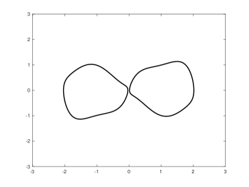
Figure 1: General geometry.

Let $H$ be a given entire harmonic function in $\mathbb{R}^{2}$. We consider the following problem

$$\begin{cases}\Delta u=0&\quad\mbox{in }\mathbb{R}^{2}\backslash\overline{(D_{1}\cup D_{2})},\\ u=\lambda_{j}(\mbox{constant})&\quad\mbox{on }\partial D_{j},~{}j=1,2,\\ u-H(x)=O(|x|^{-1})&\quad\mbox{as }|x|\to\infty,\end{cases}$$ (1.1)

where the constants $\lambda_{j}$ are determined by the conditions

$$\int_{\partial D_{j}}\frac{\partial u_{\epsilon}}{\partial\nu}\Big{|}_{+}ds=0,~{}j=1,2.$$

Here and throughout this paper, $\nu$ denotes the unit outward normal on $\partial D_{j}$. The notations $|_{+}$ and $|_{-}$ are for limits from outside and inside of inclusions, respectively. It is worth mentioning that the constants $\lambda_{1}$ and $\lambda_{2}$ may or may not be the same depending on the applied field $H$.

When $D_{1}$ and $D_{2}$ are closely located, the gradient of the solution $u$ may become arbitrarily large (blow-up) as the distance between two inclusions tends to zero. Two inclusions $D_{1}$ and $D_{2}$ may represent two perfect conductors of infinite conductivity embedded in a relatively weak conducting matrix. The solution $u$ represents the electric potential and the gradient of it represents the electric field. In two dimension, $D_{1}$ and $D_{2}$ may also represent the two dimensional cross-sections of two parallel elastic fibers embedded in an infinite elastic matrix. In this case, the solution $u$ represents the out-of-plane elastic displacement, and the gradient of the solution is proportional to the shear stress. When the inclusions are fiber-reinforced composites that are densely packed, the stress concentration may occur and cause material failure due to the damage of fiber composites. Thus, it is important to quantitatively understand the stress concentration. This problem was first raised in [6]. During the last two decades or more, significant development on this problem has been developed. It has been proved that the gradient blow-up rate is $\epsilon^{-1/2}$ in two dimensions [3, 4, 5, 7, 9, 11, 12, 18, 23, 24, 25], and $|\epsilon\ln\epsilon|^{-1}$ in three dimensions [8, 9, 10, 16, 19, 20, 21, 22], see [13] for more references.

Due to the stress concentration near the narrow region between two inclusions, fine meshes are required to numerically compute the stress. Recently, a better understanding of the stress concentration has been proposed in [24] and used for various different circumstances [1, 14, 15, 16, 17]. It is shown that the asymptotic behavior of the gradient of the solution can be characterized by a singular function associated with two inclusions as the distance $\epsilon$ tends to zero. Using this singular function, the solution can be decomposed into a singular and a regular term. After extracting the singular term in an explicit way, it is sufficient to compute the residual term only using regular meshes. Thus, this characterization of the singular term method should have good applications in the numerical computation of the gradient of the solution. In fact, this idea was exploited numerically in [14] for the special case when two inclusions are disks. The numerical results show that the characterization of the singular term method can be effectively used for computation of the gradient in the presence of two nearly touching disks.

Motivated by the theoretical result of characterization of the singular term method and its significant implication on numerical computation of the stress, in this paper, we numerically compute the solution for two nearly touching inclusions of general shapes and show the convergence of the solution. The main difference between the computation for two general shaped nearly touching inclusions and that in [14] for disks lies in the computation of the so called stress concentration factor which is the normalized magnitude of the stress concentration, as well as in the computation of the singular function. Those two terms are explicit and of simple form for two nearly touching disks, but they are not for general shapes. In this paper, we will show how to numerically obtain these two terms for nearly touching inclusions of general shapes. In fact, it was shown in [15] that the stress concentration factor converges to a certain integral of the solution to the touching case as the distance between two inclusions tends to zero. Based on this theoretical result, we will compute the value of the stress concentration factor accurately by numerically solving the touching case. The main goal of this paper is to show through numerical simulations that the characterization of the singular term method can be efficiently used for computation of the gradient when two closely located inclusions are of general shapes.

This paper is organized as follows. In section 2, we briefly review on the characterization of the singular term method. In section 3, we show how to compute the stress concentration factor by solving the touching problem. In section 4, we give the numerical computation scheme of the characterization of singular term method and show the effectiveness of it. Some numerical examples of the computation of the solution for general shaped domains are given in Section 5. This paper ends with a short inclusion.

2 Review on the characterization of the singular term method

In this section, we briefly review the characterization of the singular term method obtained in [1, 15].

Let $D_{1}$ and $D_{2}$ be two stiff inclusions in $\mathbb{R}^{2}$ with $C^{2,\gamma}$ smooth boundaries for some $\gamma\in(0,1)$. They satisfy the geometric description in the previous section. Let $z_{1}\in\partial D_{1}$ and $z_{2}\in\partial D_{2}$ are the closest points such that $|z_{1}-z_{2}|=\mbox{dist}(D_{1},D_{2})$. Let $\epsilon:=\mbox{dist}(D_{1},D_{2})$. After rotation and translation, we assume that $z=(z_{1}+z_{2})/2$ is at the origin. We also assume that the $x_{1}$-axis is parallel to the vector $z_{2}-z_{1}$. Then

$$z_{1}=(-\epsilon/2,0)\quad\mbox{and}\quad z_{2}=(\epsilon/2,0).$$

Let $B_{j}$ be the disk osculating to $D_{j}$ at $z_{j}$ $(j=1,2)$. Let $R_{j}$ be the reflection with respect to $\partial B_{j}$, $j=1,2$, and let $p_{1}\in B_{1}$ is the fix point of the mixed reflection $R_{1}R_{2}$, and $p_{2}\in D_{2}$ be that of $R_{2}R_{1}$. Let $q$ be the singular function associated with $B_{1}$ and $B_{2}$, given as follows:

$$q(x)=\frac{1}{2\pi}\left(\ln|x-p_{1}|-\ln|x-p_{2}|\right).$$ (2.1)

It is easy to see that $\nabla q$ blows up at the order of $\epsilon^{-1/2}$ near the narrow region between two inclusions.

It is proved in [1, 15] that the solution $u$ to the problem (1.1) admits the following representation:

$$\nabla u(x)=\alpha_{0}\nabla q(x)(1+O(\epsilon^{\gamma/2}))+O(1)\quad\mbox{as}~{}\epsilon\rightarrow 0.$$ (2.2)

Since $\nabla q$ blows up at the order of $\epsilon^{-1/2}$, $\alpha_{0}\nabla q$ is the singular part of $\nabla u$. Here, $\alpha_{0}$ is the so called stress concentration factor, which is given by the solution to the touching case, namely, the case when $\epsilon=0$. In fact, it is shown in [15] that $\alpha_{0}$ can be computed in the following way. For $\rho>0$, let

$$D_{\rho}=(D_{1}^{0}\cup D_{2}^{0})\cup([-\rho,\rho]\times[-\rho,\rho]),$$ (2.3)

which is of dumbbell shape. Let $u_{\rho}$ be the solution to

$$\begin{cases}\Delta u_{\rho}=0\quad\mbox{in }\mathbb{R}^{d}\backslash\overline{D}_{\rho},\\ u_{\rho}=\lambda_{\rho}(\mbox{constant})\quad\mbox{on }\partial D_{\rho},\\ u_{\rho}(x)-H(x)=O(|x|^{-1})\quad\quad\mbox{as }|x|\to\infty,\end{cases}$$ (2.4)

where the constant $\lambda_{\rho}$ is determined by the additional condition

$$\int_{\partial D_{\rho}}\partial_{\nu}u_{\rho}|_{+}ds=0.$$

Let

$$\alpha_{\rho}=\int_{\partial D_{1}^{0}\backslash[-2\rho,2\rho]\times[-2\rho,2\rho]}\partial_{\nu}u_{\rho}|_{+}ds.$$ (2.5)

Then there are constants $C$ and $A>0$ independent of $\rho$ such that

$$|\alpha_{0}-\alpha_{\rho}|\leq C\exp\left(-\frac{A}{\rho}\right).$$ (2.6)

By (2.6), one can obtain an accurate approximation of the stress concentration factor $\alpha_{0}$ by computing (2.5) through the touching case (2.4).

In particularly, if two inclusions are disks of radius $r_{1}$ and $r_{2}$, respectively, the stress concentration factor is given as

$$\alpha_{0}=\frac{4\pi r_{1}r_{2}}{r_{1}+r_{2}}(\nu\cdot\nabla H)(z).$$

However, the concentration factor could not be obtained explicitly for general shaped domain. Thanks to [3], the stress concentration factor was shown to converge to a certain integral of the solution to the touching case as the distance between two inclusions tends to zero. Based on this theoretical result, we will show how to compute the value of the stress concentration factor accurately by numerically solving the touching case in the next section.

Therefore, by (2.2), the solution $u$ to the problem (1.1) can be decomposed as a singular term and a regular term:

$$u(x)=\alpha_{0}q(x)+b(x),$$

where $q$ is given by (2.1) and

$$\|\nabla b\|_{L^{\infty}(\mathbb{R}^{2}\backslash D_{1}\cup D_{2})}\leq C$$

for a constant $C$ independent of $\epsilon$. Therefore, for the numerical computation, it is sufficient to compute $b$ only using regular meshes.

3 Computation of the stress concentration factor $\alpha_{0}$

In this section, we compute the stress concentration factor $\alpha_{0}$ by solving the touching case (2.4) using boundary element method by Matlab. We also show the convergent rate of the computation. Before doing so, we introduce some basic concepts on layer potentials.

Let

$$\Gamma(x)=\frac{1}{2\pi}\ln|x|,$$

the fundamental solution to the Laplacian in two dimensions. Let $\Omega$ be a simply connected domain with the Lipschitz boundary. The single and double layer potentials of a function $\varphi$ on $\partial\Omega$ are defined to be

$$\mathcal{S}_{\partial\Omega}[\varphi](x) :=\int_{\partial\Omega}\Gamma(x-y)\varphi(y)\,ds(y),\quad x\in\mathbb{R}^{2},$$

$$\mathcal{D}_{\partial\Omega}[\varphi](x) :=\int_{\partial\Omega}\partial_{\nu_{y}}\Gamma(x-y)\varphi(y)\,ds(y),\quad x\in\mathbb{R}^{2}\setminus\partial\Omega,$$

where $\partial_{\nu_{y}}$ denotes outward normal derivative with respect to $y$-variables. It is well known (see, for example, [2]) that the single and double layer potentials satisfy the following jump relations:

$$\partial_{\nu}\mathcal{S}_{\partial\Omega}[\varphi](x)\Big{|}_{\pm} =(\pm\displaystyle\frac{1}{2}I+\mathcal{K}_{\partial\Omega}^{*})[\varphi](x),\quad\mbox{a.e. }x\in\partial\Omega,$$ (3.1)

$$\mathcal{D}_{\partial\Omega}[\varphi](x)\big{|}_{\pm} =(\mp\displaystyle\frac{1}{2}I+\mathcal{K}_{\partial\Omega})[\varphi](x),\quad\mbox{a.e. }x\in\partial\Omega,$$ (3.2)

where the operator $\mathcal{K}_{\partial\Omega}$ on $\partial\Omega$ is defined by

$$\mathcal{K}_{\partial\Omega}[\varphi](x)=\mbox{p.v.}\int_{\partial\Omega}\partial_{\nu_{y}}\Gamma(x-y)\varphi(y)\,ds(y),$$

and $\mathcal{K}_{\partial\Omega}^{*}$ is the $L^{2}$-adjoint of $\mathcal{K}_{\partial\Omega}$. Here, p.v. stands for the Cauchy principal value.

The stress concentration factor can be precisely estimated by the integral (2.5) through solving the touching problem (2.4), which is demonstrated in the previous section. By layer potential techniques, the solution $u_{\rho}$ to (2.4) can be represented as

$$u_{\rho}(x)=H(x)+\mathcal{S}_{\partial D_{\rho}}[\psi](x),\quad x\in\mathbb{R}^{2}\backslash\overline{D}_{\rho},$$ (3.3)

for $\psi\in L^{2}_{0}(\partial D_{\rho})$, where $L^{2}_{0}$ denotes the set of $L^{2}$ functions with mean zero. Since $u_{\rho}$ is constant on $\partial D_{\rho}$, $\psi$ should satisfy

$$\frac{\partial H}{\partial\nu}+\frac{\partial}{\partial\nu}\mathcal{S}_{\partial D_{\rho}}[\psi]\Big{|}_{-}=0\quad\mbox{on}~{}\partial D_{\rho},$$

which, according to (3.1), can be written as

$$\frac{\partial H}{\partial\nu}+\left(-\frac{1}{2}I+\mathcal{K}^{*}_{\partial D_{\rho}}\right)[\psi]=0\quad\mbox{on}~{}\partial D_{\rho}.$$ (3.4)

Taking outward normal derivative of (3.3), and by the jump relation (3.1), we have

$$\frac{\partial u_{\rho}}{\partial\nu}\Big{|}_{+}=\frac{\partial H}{\partial\nu}+\left(\frac{1}{2}I+\mathcal{K}^{*}_{\partial D_{\rho}}\right)[\psi]\quad\mbox{on}~{}\partial D_{\rho}.$$ (3.5)

In view of (3.4), then (3.5) becomes

$$\frac{\partial u_{\rho}}{\partial\nu}\Big{|}_{+}=\psi\quad\mbox{on}~{}\partial D_{\rho}.$$ (3.6)

Hence by (2.5) and (3.6), we have

$$\alpha_{\rho}=\int_{\partial D_{1}^{0}\backslash[-2\rho,2\rho]\times[-2\rho,2\rho]}\psi ds,$$ (3.7)

where $\psi$ is given by (3.4) as follows

$$\psi=\left(\frac{1}{2}I-\mathcal{K}^{*}_{\partial D_{\rho}}\right)^{-1}\left[\frac{\partial H}{\partial\nu}\right].$$

The density function $\psi$ can be uniquely solved. In fact, it is well known, see for example [2], that the operator $\lambda I-\mathcal{K}^{*}_{\partial D_{\rho}}$ is one to one on $L^{2}_{0}(\partial D_{\rho})$ if $|\lambda|\geq 1/2$ when $D_{\rho}$ is a bounded Lipschitz domain.

We now compute (3.7) using boundary element method. For example, let $D_{1}$ and $D_{2}$ be two elliptic inclusions of the same major axis $a=2$ and minor axis $b=1$, centered at $(-a-\epsilon/2,0)$ and $(a+\epsilon/2,0)$, respectively, where $\epsilon=0.01$. The domain $D_{\rho}$ which is defined by (2.3) is the dumbbell shaped domain shown in Figure 2.

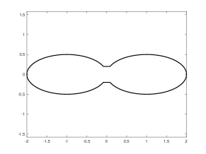
Figure 2: $D_{\rho}$ for two touching ellipses.

Discretize each boundary of $D_{j}$, $j=1,2$ into $N$ points and each connecting segment between $D_{1}$ and $D_{2}$ into $N/16$ points.

Firstly, we fix $\rho=0.05$ in (3.7) and change the values of the grids number $N$ with $N=256,512,1024,2048,4096$. Figure 3 shows the numerical result of $\alpha_{\rho}$ for different values of $N$. One can easily see that $\alpha_{\rho}$ converges as the number of grids points increases. Denote $\alpha_{*}$ as the value of $\alpha_{\rho}$ with finer grids $N=4096$. We then compare each $\alpha_{\rho}$ with $\alpha_{*}$. The relative error is shown in Figure 3 (Middle). The convergent rate is shown in Figure 3 (Right). One can see that $\alpha_{\rho}$ converges very fast as $N$ increases.

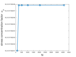
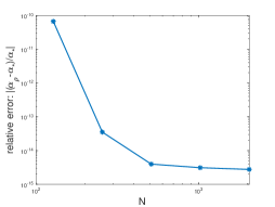
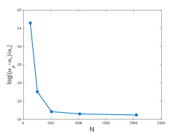
Figure 3: Left: $\alpha_{\rho}$ for different values of the grids number $N$. Middle: The relative error: $|(\alpha_{\rho}-\alpha_{*})/\alpha_{*}|$. Right: The convergent rate: $\log|(\alpha_{\rho}-\alpha_{*})/\alpha_{*}|$.

Secondly, we fix $N=512$ and change $\rho$ from $0.3$ to $0.1$. Figure 4 shows the numerical values of $\alpha_{\rho}$ for different values of $\rho$. From the left-hand side figure one can see that $\alpha_{\rho}$ converges as $\rho$ decreases. Denote $\alpha_{*}$ as the value of $\alpha_{\rho}$ when $\rho=0.1$. Then the relative errors of $\alpha_{\rho}$ and the convergent rate is shown in the middle and right-hand side figure of Figure 4, respectively. One can also see that $\alpha_{\rho}$ converges very fast as $\rho$ decreases.

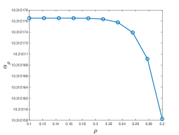
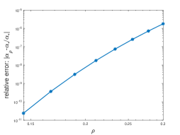
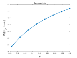
Figure 4: Left: $\alpha_{\rho}$ for different values of $\rho$. Middle: The relative error: $|(\alpha_{\rho}-\alpha_{*})/\alpha_{*}|$. Right: The convergent rate: $\log|(\alpha_{\rho}-\alpha_{*})/\alpha_{*}|$.

Figure 3 and Figure 4 both show that we can obtain accurate value of the stress concentration factor by numerical computation.

4 Numerical computations

In this section, we provide numerical scheme on the computation of the solution to (1.1) using characterization of the singular term method. We show that it can be efficiently used for the computation of the stress concentration by comparing the convergent rate with the solution computed using layer potential techniques in a direct way. The boundary element method is used for both methods.

Before providing the numerical scheme, we first derive the related system of integral equations.

4.1 System of the integral equations

Let $D_{1}$ and $D_{2}$ be the same as in the previous section. Let $B_{j}$ be the disk osculating to $D_{j}$ at $z_{j}$ ($j=1,2$), where $z_{1}=(-\epsilon/2,0)$ and $z_{2}=(\epsilon/2,0)$. Let $\kappa_{j}$ be the curvature of $D_{j}$ at $z_{j}$. Then the radius of $B_{j}$ is $r_{j}=1/\kappa_{j}$, $j=1,2$. Let $c_{j}$ be the center point of the disk $B_{j}$, $j=1,2$.

Define singular function $q$ in the spirit of (2.1) as follows

$$q(x)=\frac{1}{2\pi}\left(\ln|x-p_{1}|-\ln|x-p_{2}|-\ln|x-c_{1}|+\ln|x-c_{2}|\right),$$ (4.1)

for $x\in\mathbb{R}^{2}\backslash\overline{(D_{1}\cup D_{2})}$, where $p_{1}$ and $p_{2}$ are two fix points of the mixed reflection with respect to $\partial B_{j}$, $j=1,2$. In fact, it is shown in [24, 25] that the fixed points $p_{1}$ and $p_{2}$ are given by

$$p_{1}=\left(-\sqrt{2}\sqrt{\frac{r_{1}r_{2}}{r_{1}+r_{2}}}\sqrt{\epsilon}+O(\epsilon),0\right)\quad\mbox{and}\quad p_{2}=\left(\sqrt{2}\sqrt{\frac{r_{1}r_{2}}{r_{1}+r_{2}}}\sqrt{\epsilon}+O(\epsilon),0\right).$$ (4.2)

In view of (2.2), we look for a solution $u$ to (1.1) in the following form

$$u(x)=\alpha_{0}q(x)+H(x)+\mathcal{S}_{\partial D_{1}}[\phi_{1}](x)+\mathcal{S}_{\partial D_{2}}[\phi_{2}](x),\quad x\in\mathbb{R}^{2}\backslash\overline{(D_{1}\cup D_{2})},$$ (4.3)

where $(\phi_{1},\phi_{2})\in L^{2}_{0}(\partial D_{1})\times L^{2}_{0}(\partial D_{2})$ are to be determined. It is worth mentioning that the gradient of $H+\mathcal{S}_{\partial D_{1}}[\phi_{1}]+\mathcal{S}_{\partial D_{2}}[\phi_{2}]$ is bounded on $\mathbb{R}^{2}\backslash\overline{(D_{1}\cup D_{2})}$ according to (2.2), and hence $\|\phi_{1}\|_{L^{\infty}(\partial D_{1})}$ and $\|\phi_{2}\|_{L^{\infty}(\partial D_{2})}$ are bounded regardless of $\epsilon$. We use the fact that $\frac{\partial u}{\partial\nu}|_{-}=0$ on $\partial D_{j}$, $j=1,2$ to find the integral equations for $(\phi_{1},\phi_{2})$. In order to do so, we take harmonic extension of $u$ toward the interior of $D_{1}\cup D_{2}$. Note that $H$, $\mathcal{S}_{\partial D_{1}}[\phi_{1}]$ and $\mathcal{S}_{\partial D_{2}}[\phi_{2}]$ are continuous in $\mathbb{R}^{2}$ and harmonic in $D_{1}\cup D_{2}$. Hence, it remains to find the harmonic extension of $q$ toward the interior of $D_{1}\cup D_{2}$.

Let $q_{j}$ be the harmonic extension of $q$ towards the interior of $D_{j}$, $j=1,2$, respectively. Then $q_{j}$ should satisfy the following Dirichlet problem:

$$\begin{cases}\Delta q_{j}(x)=0\quad\mbox{in}~{}D_{j},\\ q_{j}(x)=q_{j}|_{\partial D_{j}},\end{cases}$$ (4.4)

where the boundary data is given explicitly by (4.1):

$$q_{j}|_{\partial D_{j}}=\frac{1}{2\pi}\left(\ln|x-p_{1}|-\ln|x-p_{2}|-\ln|x-c_{1}|+\ln|x-c_{2}|\right)\quad\mbox{on}~{}\partial D_{j}.$$

By numerically solving (4.4) for each $j=1,2$, one can obtain the interior harmonic extension of the singular function $q_{j}$ in $D_{j}$. Let

$$q^{G}(x)=\begin{cases}q_{1}(x)&~{}\mbox{in}~{}D_{1},\\ q_{2}(x)&~{}\mbox{in}~{}D_{2},\\ q(x)&~{}\mbox{in}~{}\mathbb{R}^{2}\backslash\overline{(D_{1}\cup D_{2})}.\end{cases}$$

Then $q^{G}$ is continuous in $\mathbb{R}^{2}$ and harmonic in $D_{1}$ and $D_{2}$ as well as in $\mathbb{R}^{2}\backslash\overline{(D_{1}\cup D_{2})}$.

Define

$$u^{G}(x)=\alpha_{0}q^{G}(x)+H(x)+\mathcal{S}_{\partial D_{1}}[\phi_{1}](x)+\mathcal{S}_{\partial D_{2}}[\phi_{2}](x),\quad x\in\mathbb{R}^{2}.$$

Then $u^{G}$ is continuous in $\mathbb{R}^{2}$ and harmonic in $D_{1}$, $D_{2}$ and $\mathbb{R}^{2}\backslash\overline{(D_{1}\cup D_{2})}$. Since $u^{G}$ is constant on $\partial D_{j}$, $j=1,2$, $u^{G}$ should be constant in $D_{j}$, $j=1,2$. Taking inward normal derivative of $u^{G}$ on $\partial D_{j}$ and by the jump relation (3.1), we obtain the following integral equations for $(\phi_{1},\phi_{2})$:

$$\begin{cases}\displaystyle\left(-\frac{1}{2}I+\mathcal{K}_{\partial D_{1}}^{*}\right)[\phi_{1}]+\frac{\partial}{\partial\nu_{D_{1}}}\mathcal{S}_{\partial D_{2}}[\phi_{2}]=-\frac{\partial H}{\partial\nu_{D_{1}}}-\alpha_{0}\frac{\partial q_{1}}{\partial\nu_{D_{1}}}\Big{|}_{-}&~{}\mbox{on}~{}\partial D_{1},\\[10.00002pt] \displaystyle\frac{\partial}{\partial\nu_{D_{2}}}\mathcal{S}_{\partial D_{1}}[\phi_{1}]+\left(-\frac{1}{2}I+\mathcal{K}_{\partial D_{2}}^{*}\right)[\phi_{2}]=-\frac{\partial H}{\partial\nu_{D_{2}}}-\alpha_{0}\frac{\partial q_{2}}{\partial\nu_{D_{2}}}\Big{|}_{-}&~{}\mbox{on}~{}\partial D_{2},\end{cases}$$ (4.5)

where $\frac{\partial q_{j}}{\partial\nu_{D_{j}}}\big{|}_{-}$, $j=1,2$, can be obtained by solving (4.4) numerically. The density functions $(\phi_{1},\phi_{2})\in L^{2}_{0}(\partial D_{1})\times L^{2}_{0}(\partial D_{2})$ can be uniquely determined by solving the system of integral equations (4.5). In fact, denote

$$\mathbb{I}=\begin{bmatrix}I&0\\ 0&I\end{bmatrix},\quad\mathbb{K}^{*}=\begin{bmatrix}\mathcal{K}_{\partial D_{1}}^{*}&\frac{\partial}{\partial\nu_{D_{1}}}\mathcal{S}_{\partial D_{2}}\\ \frac{\partial}{\partial\nu_{D_{2}}}\mathcal{S}_{\partial D_{1}}&\mathcal{K}_{\partial D_{2}}^{*}\end{bmatrix},$$

then $-\frac{1}{2}\mathbb{I}+\mathbb{K}^{*}$ is invertible on $L^{2}_{0}(\partial D_{1})\times L^{2}_{0}(\partial D_{2})$, which is shown in, for example, [1].

To solve $(\phi_{1},\phi_{2})$ from (4.5), discretize each boundary $\partial D_{j}$, $j=1,2$ into $N$ points, respectively. Let $x_{j}^{k}$, $k=1,\dots,N$, be the nodal points on $\partial D_{j}$. Then (4.5) becomes

$$\left(-\frac{1}{2}I+A\right)\begin{bmatrix}\phi_{1}\\ \phi_{2}\end{bmatrix}=\begin{bmatrix}Y_{1}\\ Y_{2}\end{bmatrix},$$

where

$$I=\begin{bmatrix}I_{N}&0\\ 0&I_{N}\end{bmatrix},\quad A=\begin{bmatrix}A_{11}&A_{12}\\ A_{21}&A_{22}\end{bmatrix},$$ (4.6)

and

$$Y_{1}=-\begin{bmatrix}\frac{\partial H}{\partial\nu_{D_{1}}}(x_{1}^{1})+\alpha_{0}\frac{\partial q_{1}}{\partial\nu_{D_{1}}}\big{|}_{-}(x_{1}^{1})\\ \vdots\\ \frac{\partial H}{\partial\nu_{D_{1}}}(x_{1}^{N})+\alpha_{0}\frac{\partial q_{1}}{\partial\nu_{D_{1}}}\big{|}_{-}(x_{1}^{N})\end{bmatrix},\quad Y_{2}=-\begin{bmatrix}\frac{\partial H}{\partial\nu_{D_{2}}}(x_{2}^{1})+\alpha_{0}\frac{\partial q_{2}}{\partial\nu_{D_{2}}}\big{|}_{-}(x_{2}^{1})\\ \vdots\\ \frac{\partial H}{\partial\nu_{D_{2}}}(x_{2}^{N})+\alpha_{0}\frac{\partial q_{2}}{\partial\nu_{D_{2}}}\big{|}_{-}(x_{2}^{N})\end{bmatrix}.$$

Here $A$ is the evaluation of the kernel of $\mathbb{K}^{*}$. It is worth mentioning that the matrix $-\frac{1}{2}I+A$ has small singular values and the condition number of $A$ becomes worse as $\epsilon$ tends to zero, as shown in Figure 5.

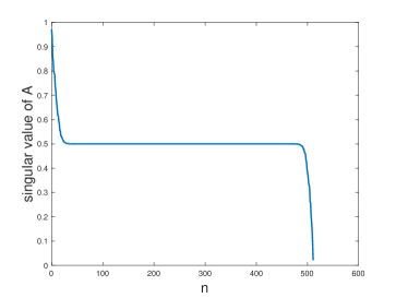
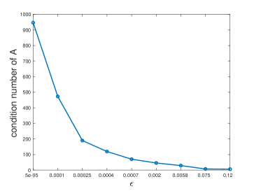
Figure 5: Left: the singular values of $A$ in the decreasing order of $n$ when $\epsilon$ is $0.01$. Right: the condition numbers of $A$ as the distance $\epsilon$ tends to $0$. The dimension of $A$ is $512\times 512$.

However, $\|\phi_{1}\|_{L^{\infty}(\partial D_{1})}$ and $\|\phi_{2}\|_{L^{\infty}(\partial D_{2})}$ are bounded regardless of $\epsilon$.

We compute $(\phi_{1},\phi_{2})$ with $N=256,512,1024,2048,4096$ equi-spaced points on $\partial D_{j}$, $j=1,2$, respectively. And then they are compared with the solution on the finer grid with $N=4096$. Denote $(\phi_{1}^{*},\phi_{2}^{*})$ as the solution with grid number $N=4096$. Let

$$\frac{\|\phi_{1}-\phi_{1}^{*}\|_{L^{2}(\partial D_{1})}}{2\|\phi_{1}^{*}\|_{L^{2}(\partial D_{1})}}+\frac{\|\phi_{2}-\phi_{2}^{*}\|_{L^{2}(\partial D_{2})}}{2\|\phi_{2}^{*}\|_{L^{2}(\partial D_{2})}}$$

be the relative $L^{2}$-errors of $(\phi_{1},\phi_{2})$ compared with $(\phi_{1}^{*},\phi_{2}^{*})$. Figure 6 (Left) shows that the relative errors decrease as the grid number $N$ increases. Figure 6 (Right) shows the logarithm of the relative error. One can see that $(\phi_{1},\phi_{2})$ converges very fast.

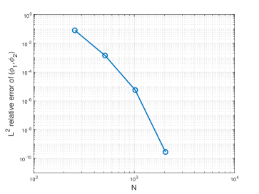
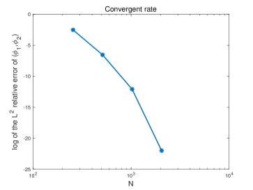
Figure 6: Left: Relative error of $(\phi_{1},\phi_{2})$. Right: Logarithm of the relative error of $(\phi_{1},\phi_{2})$.

4.2 Numerical scheme and effectiveness of the method

In this subsection we give the numerical scheme on the computation of the solution using characterization of the singular term method in the following Algorithm 1. We show the effectiveness of this method by comparing the convergent rate with the solution computed using layer potential techniques in a direct way.

Algorithm 1 Numerical scheme

Step 1. Look for the solution to (1.1) in terms of the following form:

$$u(x)=\alpha_{0}q(x)+H(x)+\mathcal{S}_{\partial D_{1}}[\phi_{1}](x)+\mathcal{S}_{\partial D_{2}}[\phi_{2}](x),\quad x\in\mathbb{R}^{2}\backslash\overline{(D_{1}\cup D_{2})},$$

where $q$ is given by (4.1) and $\alpha_{0}$, $(\phi_{1},\phi_{2})$ are to be computed.

Step 2. Compute the stress concentrator factor $\alpha_{0}$ by considering the touching case (2.4):

• Discretize $\partial D_{\rho}$ into $2N+N/8$ points;

• Solve integral equation (3.4) numerically;

• Obtain $\alpha_{0}$ through (3.7).

Step 3. Compute the density functions $(\phi_{1},\phi_{2})$ through (4.5):

• Discretize each $\partial D_{j}$, $j=1,2$ into $N$ points, respectively;

• Compute the inward normal derivative $\frac{\partial q_{j}}{\partial\nu}\big{|}_{-}$, $j=1,2$ by solving the Dirichlet problem (4.4), respectively;

• Obtain $(\phi_{1},\phi_{2})$ by numerically solving (4.5).

Step 4. Plot $u$.

Denote $u^{deco}$ the solution computed following Algorithm 1. Denote $u^{dire}$ the solution to (1.1) by direct compution method. In fact, $u^{dire}$ can be written as

$$u(x)=H(x)+\mathcal{S}_{\partial D_{1}}[\psi_{1}](x)+\mathcal{S}_{\partial D_{2}}[\psi_{2}](x),\quad x\in\mathbb{R}^{2}\backslash{(D_{1}\cup D_{2})},$$

where two density functions $(\psi_{1},\psi_{2})\in L^{2}_{0}(\partial D_{1})\times L^{2}_{0}(\partial D_{2})$ satisfy

$$\left(-\frac{1}{2}I+A\right)\begin{bmatrix}\psi_{1}\\ \psi_{2}\end{bmatrix}=-\begin{bmatrix}\frac{\partial H}{\partial\nu_{D_{1}}}\\[4.30554pt] \frac{\partial H}{\partial\nu_{D_{2}}}\end{bmatrix},$$

where $A$ is given by (4.6). Note that the density functions $\psi_{j}$, $j=1,2$ are as big as $1/\sqrt{\epsilon}$ near the origin point $(0,0)$ when $\nu\cdot\nabla H\neq 0$. Thus, applying single layer on $\psi_{j}$, $j=1,2$, the error in the discretization of the single layer potential should become significant.

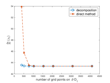
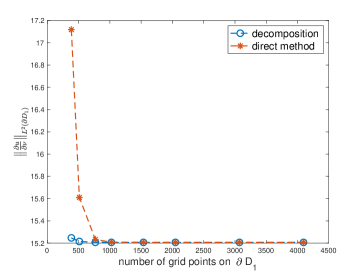
Figure 7: Left: $\frac{\partial u^{deco}}{\partial\nu}$ and $\frac{\partial u^{dire}}{\partial\nu}$ at the closest point $z_{1}$; Right: $L^{2}$-norm of $\frac{\partial u^{deco}}{\partial\nu}$ and $\frac{\partial u^{dire}}{\partial\nu}$.

Let $D_{1}$ and $D_{2}$ be the same as in Section 3. Let the distance between $D_{1}$ and $D_{2}$ be $\epsilon=0.01$. Let $z_{1}=(-\epsilon/2,0)$ and $z_{2}=(\epsilon/2,0)$ be the closest points on $\partial D_{1}$ and $\partial D_{2}$. The background potential is given by $H(x)=x_{1}$. Discretize each boundary $\partial D_{j}$, $j=1,2$ into $N$ points. Figure 7 (Left) shows the normal derivative of $u^{dire}$(orange) and $u^{deco}$(blue) at $z_{1}$ for different values of $N$. Figure 7 (Right) shows the $L^{2}$-norm of those on boundary $\partial D_{1}$. One can see that both methods obtain convergent result, but the direct computation method needs finer meshes to obtain the accurate result. In fact, from Figure 7 one can see that the direct computation method needs at least $N=1024$ nodes on each boundary to obtain good result, whereas the characterization of the singular term method needs only needs $N=512$. This further indicates that the scale of the line element of the discretization should be comparable with the scale of $\epsilon$ using the direct computation method, whereas the characterization of the singular term method does not limit to this restriction.

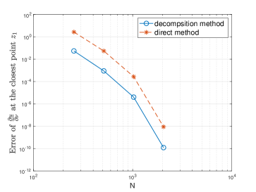
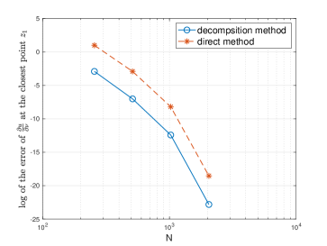
Figure 8: Left: the relative errors of $\frac{\partial u^{dire}}{\partial\nu}$ and $\frac{\partial u^{deco}}{\partial\nu}$ compared to $\frac{\partial u^{*}}{\partial\nu}$; Right: the logarithm of the relative errors. The distance $\epsilon=0.01$. The background potential is given by $H(x)=x_{1}$.

From Figure 7, one can see that both methods obtain accurate results when the number of grid $N$ is sufficiently large. Hence, we assume that upon $N=4096$ the solution is regarded as the exact solution and denote it by $u^{*}$.

Fix $\epsilon=0.01$. To show the effectiveness of the characterization of the singular term method, we compare the normal derivative $\frac{\partial u^{dire}}{\partial\nu}$ and $\frac{\partial u^{deco}}{\partial\nu}$, with $\frac{\partial u^{*}}{\partial\nu}$, at the closest point $z_{1}$, for different values of $N=256,512,1024,2048$. Let

$$\frac{\left|\frac{\partial u^{dire}}{\partial\nu_{D_{1}}}(z_{1})-\frac{\partial u^{*}}{\partial\nu_{D_{1}}}(z_{1})\right|}{\left|\frac{\partial u^{*}}{\partial\nu_{D_{1}}}(z_{1})\right|}\quad\mbox{and}\quad\frac{\left|\frac{\partial u^{deco}}{\partial\nu_{D_{1}}}(z_{1})-\frac{\partial u^{*}}{\partial\nu_{D_{1}}}(z_{1})\right|}{\left|\frac{\partial u^{*}}{\partial\nu_{D_{1}}}(z_{1})\right|}$$

be the relative errors of $\frac{\partial u^{dire}}{\partial\nu}$ and $\frac{\partial u^{deco}}{\partial\nu}$ at the closest point $z_{1}$, respectively. Figure 8 (Left) shows that the relative errors of $\frac{\partial u^{dire}}{\partial\nu}$ and $\frac{\partial u^{deco}}{\partial\nu}$ both decrease as the grid number $N$ increases. However, the error of $\frac{\partial u^{deco}}{\partial\nu}$ is much smaller than that of $\frac{\partial u^{dire}}{\partial\nu}$. The convergent speed of $\frac{\partial u^{deco}}{\partial\nu}$ is faster than that of $\frac{\partial u^{dire}}{\partial\nu}$, which is shown in Figure 8 (Right).

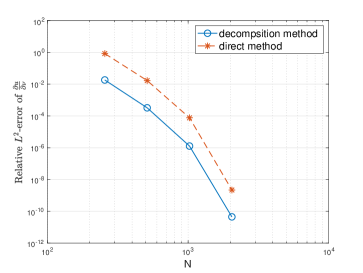
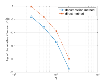
Figure 9: Left: The relative $L^{2}$-errors of $\frac{\partial u^{dire}}{\partial\nu}$ and $\frac{\partial u^{deco}}{\partial\nu}$, respectively. Right: The logarithm of the relative $L^{2}$-error.

We also compare the relative $L^{2}$-errors of $\frac{\partial u^{dire}}{\partial\nu}$ and $\frac{\partial u^{deco}}{\partial\nu}$, respectively, for different grid numbers $N=256,512,1024,2048$. Let

$$\frac{\|\frac{\partial u^{dire}}{\partial\nu_{D_{1}}}-\frac{\partial u^{*}}{\partial\nu_{D_{1}}}\|_{L^{2}(\partial D_{1})}}{2\|\frac{\partial u^{*}}{\partial\nu_{D_{1}}}\|_{L^{2}(\partial D_{1})}}+\frac{\|\frac{\partial u^{dire}}{\partial\nu_{D_{2}}}-\frac{\partial u^{*}}{\partial\nu_{D_{2}}}\|_{L^{2}(\partial D_{2})}}{2\|\frac{\partial u^{*}}{\partial\nu_{D_{2}}}\|_{L^{2}(\partial D_{2})}}$$

and

$$\frac{\|\frac{\partial u^{deco}}{\partial\nu_{D_{1}}}-\frac{\partial u^{*}}{\partial\nu_{D_{1}}}\|_{L^{2}(\partial D_{1})}}{2\|\frac{\partial u^{*}}{\partial\nu_{D_{1}}}\|_{L^{2}(\partial D_{1})}}+\frac{\|\frac{\partial u^{deco}}{\partial\nu_{D_{2}}}-\frac{\partial u^{*}}{\partial\nu_{D_{2}}}\|_{L^{2}(\partial D_{2})}}{2\|\frac{\partial u^{*}}{\partial\nu_{D_{2}}}\|_{L^{2}(\partial D_{2})}}$$

be the relative $L^{2}$-errors of $\frac{\partial u^{dire}}{\partial\nu}$ and $\frac{\partial u^{deco}}{\partial\nu}$, respectively. Figure 9 (Left) shows that the relative $L^{2}$-errors of both methods decrease as the grid number $N$ increases, while the error of $\frac{\partial u^{deco}}{\partial\nu}$ is much smaller than that of $\frac{\partial u^{dire}}{\partial\nu}$. Figure 9 (Right) shows that the convergent rate of $\frac{\partial u^{deco}}{\partial\nu}$ is faster than that of $\frac{\partial u^{dire}}{\partial\nu}$, which indicates that the characterization of the singular term method is more effective.

$\epsilon$	$\frac{\partial u^{deco}}{\partial\nu}\left(z_{1}\right)$
0.018	31.745002
0.016	33.802881
0.014	36.292441
0.012	39.387485
0.010	43.378565
0.008	48.798534
0.006	56.770126
0.004	70.326757

Table 1: The value of $\frac{\partial u^{deco}}{\partial\nu}$ at the closest point $z_{1}$, for different $\epsilon$.

If we fix the number of grid points $N=1024$ and vary the distance $\epsilon$ from $0.018$ to $0.004$. Table 1 lists the values of the normal flux of $u^{deco}$ at the closest point $z_{1}$ for different values of $\epsilon$. The values are plotted as the blue star points in Figure 10. The blow up rate of $\frac{\partial u^{deco}}{\partial\nu}$ is known to be $1/\sqrt{\epsilon}$ in two dimension. In fact, by (4.3), we have

$$\frac{\partial u^{deco}}{\partial\nu}(z_{1})=\alpha_{0}\frac{\partial q}{\partial\nu}(z_{1})+O(1).$$

By (4.1) and (4.2), the above formula becomes

$$\frac{\partial u^{deco}}{\partial\nu}(z_{1})=\frac{\alpha_{0}}{2\pi}\left(\frac{z_{1}-p_{1}}{|z_{1}-p_{1}|^{2}}-\frac{z_{1}-p_{2}}{|z_{1}-p_{2}|^{2}}\right)+O(1).$$

The concentration stress factor $\alpha_{0}$ is $10.312176$ which is given by Figure 3 and Figure 4. Together with the explicit value of $r_{1}=1/2$, $r_{2}=1/2$ in (4.2), we have

$$\frac{\partial u^{deco}}{\partial\nu}(z_{1})=4.632\epsilon^{-1/2}+O(1).$$ (4.7)

We now confirm the blow up rate $\epsilon^{-1/2}$ and its coefficient in (4.7) by fitting the values of $\frac{\partial u^{deco}}{\partial\nu}$ in Table 1 with $\epsilon$ decreases from $0.018$ to $0.004$. The result is plotted as the red curve in Figure 10. One can clearly see that the blow up rate is $\epsilon^{-1/2}$ and the coefficient of the fitting curve $4.593$ matches well with the coefficient in (4.7). This result is interesting and reasonable.

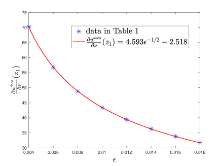
Figure 10: Fitting curve and $\frac{\partial u^{deco}}{\partial\nu}$ at the closest point $z_{1}$ for different $\epsilon$.

5 Numerical examples

In this section, we present some examples of numerical experiments on various different shapes of two closely located inclusions. The distance between two inclusions is $\epsilon=0.01$.

Firstly, let $D_{1}$ and $D_{2}$ be two elliptic inclusions of the same major axis $a=2$ and minor axis $b=1$, centered at $(-a-\epsilon/2,0)$ and $(a+\epsilon/2,0)$, respectively. Discretize each boundary $\partial D_{j}$, $j=1,2$, into 256 grid nodes. Applying linear field $H(x)=x_{1}$, Figure 11 (Left) shows the uniformly spaced contour level curves. Applying linear field $H(x)=x_{2}$, one can see from Figure 11 (Middle) that the gradient does not blow up. Let $H(x)=x_{1}+x_{2}$, Figure 11 (Right) shows the uniformly spaced contour level curves.

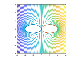
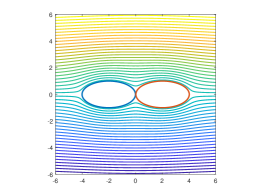
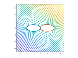
Figure 11: Level curves of the stiff inclusions of elliptic shapes. Left: $H(x)=x_{1}$; Middle: $H(x)=x_{2}$; Right: $H(x)=x_{1}+x_{2}$.

Secondly, let $D_{1}$ be an ellipse with the major axis $a=2$ and minor axis $b=1$, centered at $(-a-\epsilon/2,0)$, and let $D_{2}$ be a circle of radius $r=1$ centered at $(r+\epsilon/2,0)$. Figure 12 shows the uniformly spaced contour level curves when $H(x)=x_{1}$, $H(x)=x_{2}$ and $H(x)=x_{1}+x_{2}$, respectively.

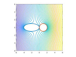
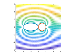
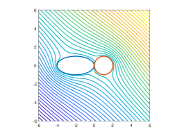
Figure 12: Level curves of the stiff inclusions of elliptic and disk shapes. Left: $H(x)=x_{1}$; Middle: $H(x)=x_{2}$; Right: $H(x)=x_{1}+x_{2}$.

As the final example, Figure 13 shows the uniformly spaced contour level curves for two stiff inclusions of general shape, when $H(x)=x_{1}$, $H(x)=x_{2}$ and $H(x)=x_{1}+x_{2}$, respectively. The boundaries of two inclusions are given by the following parametrization functions for $\theta\in[0,2\pi)$:

$$\begin{cases}x_{1}=-\frac{\epsilon}{2}-1+\cos(\theta),\\ x_{2}=-\frac{1}{12}+\sin(\theta)-\frac{1}{6}\sin(2\theta)+\frac{1}{12}\cos(4\theta).\end{cases}$$

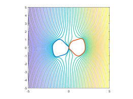
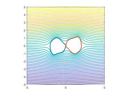
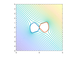
Figure 13: Level curves of the stiff inclusions of general shape. Left: $H(x)=x_{1}$; Middle: $H(x)=x_{2}$; Right: $H(x)=x_{1}+x_{2}$.

6 Conclusion

In this paper, we show through numerical simulations that the computation of the stress concentration between closely located stiff inclusions of general shapes can be realized by using only regular meshes. Using the characterization of the singular term method, we can decompose the solution into a singular and a regular term. After extracting the singular in a precise way, we can compute the remaining term using regular meshes. The key point in our computation lies in the computation of the stress concentration factor as well as the singular term. We have shown that the computation of the stress concentration factor converges very fast. By comparing the convergent rate with the solution computed using layer potential techniques in a direct way, we conclude that the characterization of the singular term method can be used effectively for the computation of the solution.

References

- [1] H. Ammari, G. Ciraolo, H. Kang, H. Lee and K. Yun, Spectral Analysis of the Neumann-Poincaré Operator and Characterization of the Stress Concentration in Anti-Plane Elasticity, Arch. Rational Mech. Anal. 208, 275–304 (2013).
- [2] H. Ammari and H. Kang, Polarization and moment tensors, Applied Mathematical Sciences, 162, Springer, New York, 2007.
- [3] H. Ammari, H. Kang, H. Lee, J. Lee and M. Lim, Optimal bounds on the gradient of solutions to conductivity problems, J. Math. Pure Appl. 88, 307-324 (2007).
- [4] H. Ammari, H. Kang, H. Lee and H. Zribi, Decomposition theorem and fine estimates for electric fields in the presence of closely located circular inclusions, J. Differ. Equ. 247, 2897-2912 (2009).
- [5] H. Ammari, H. Kang and M. Lim, Gradient estimates for solutions to the conductivity problem, Math. Ann. 332(2), 277–286 (2005).
- [6] I. Babuka, B. Andersson, P. Smith and K. Levin, Damage analysis of fiber composites Part I: Statistical analysis on fiber scale, Comput. Methods Appl. Mech. Eng. 172, 27–77 (1999).
- [7] J. Bao, H. Li and Y. Li, Gradient estimates for solutions of the Lamé system with partially infinite coefficients, Arch. Rational Mech. Anal. 215, 307–351 (2015).
- [8] J. Bao, H. Li and Y. Li, Gradient estimates for solutions of the Lamé system with partially infinite coefficients in dimensions greater than two, Adv. Math. 305, 298–338 (2017).
- [9] E. Bao, Y. Li and B. Yin, Gradient estimates for the perfect conductivity problem, Arch. Ration. Mech. Anal. 193, 195–226 (2009).
- [10] E. Bao, Y. Li and B. Yin, Gradient estimates for the perfect and insulated conductivity problems with multiple inclusions, Commun. Partial Differ. Equ. 35, 1982–2006 (2010).
- [11] B. Budiansky and G. Carrier High shear stresses in stiff fiber composites, J. Appl. Mech. 51, 733–735 (1984).
- [12] E. Bonnetier and M. Vogelius, An elliptic regularity result for a composite medium with “touching” fibers of circular cross-section, SIAM J. Math. Anal. 31, 651–677 (2000).
- [13] H. Kang Quantitative analysis of field concentration in presence of closely located inclusions of high contrast, Proceedings ICM 2022.
- [14] H. Kang, M. Lim and K. Yun, Asymptotics and computation of the solution to the conductivity equation in the presence of two adjacent inclusions with extreme conductivities, J. Math. Pure. Appl. 99, 234-249 (2013).
- [15] H. Kang, H. Lee and K. Yun, Optimal estimates and asymptotics for the stress concentration between closely located stiff inclusions, Math. Ann. 363: 1281-1306 (2015).
- [16] H. Kang, H. Lee and K. Yun, Characterization of the electric field concentration between two adjacent spherical perfect conductors, SIAM J. Appl. Math. Vol. 74, No. 1, pp. 125-146 (2014).
- [17] H. Kang and S. Yu, Quantitative characterization of stress concentration in the presence of closely spaced hard inclusions in two-dimensional linear elasticity, Arch. Rational Mech. Anal. 232, 121-196 (2019).
- [18] J. Keller, Stresses in narrow regions, Trans. ASME J. Appl. Mech. 60, 1054-1056 (1993).
- [19] J. Lekner, Analytical expression for the electric field enhancement between two closely-spaced conducting spheres, J. Electrostatics 68, 299–304 (2010).
- [20] J. Lekner, Near approach of two conducting spheres: enhancement of external electric field, J. Electrostatics 69, 559–563 (2011).
- [21] J. Lekner, Electrostatics of two charged conducting spheres, J. Proc. R. Soc. A 468, 2829-2848 (2012).
- [22] M. Lim and K. Yun, Blow-up of electric fields between closely spaced spherical perfect conductors, Commun. Partial Differ. Equ. 34, 1287–1315 (2009).
- [23] M. Lim and K. Yun, Strong influence of a small fiber on shear stress in fiber-reinforced composites, J. Differ. Equ. 250, 2402–2439 (2011).
- [24] K. Yun, Estimates for electric fields blow up between closely adjacent conductors with arbitrary shape, SIAM J. Appl. Math. 67, 714-730 (2007).
- [25] K. Yun, Optimal bound on high stresses occurring between stiff fibers with arbitrary shaped cross sections, J. Math. Anal. Appl. 350, 306–312 (2009).