On the structure of wave functions in complex Chern–Simons theory

Abstract

We study the structure of wave functions in complex Chern–Simons theory on the complement of a hyperbolic knot, emphasizing the similarities with the topological string/spectral theory correspondence. We first conjecture a hidden integrality structure in the holomorphic blocks and show that this structure guarantees the cancellation of potential singularities in the full non-perturbative wave function at rational values of the coupling constant. We then develop various techniques to determine the wave function at such rational points. Finally, we illustrate our conjectures and obtain explicit results in the examples of the figure-eight and the three-twist knots. In the case of the figure-eight knot, we also perform a direct evaluation of the state integral in the rational case and observe that the resulting wave function has the features of the ground state for a quantum mirror curve.

1 Introduction

Chern–Simons (CS) theory with a complex gauge group has been an excellent laboratory for studying various aspects of quantum field theory (QFT) since it is essentially exactly solvable. In recent years, building on previous work by physicists and mathematicians, perturbative and non-perturbative methods have been introduced, making it possible to calculate various observables, and many beautiful and interesting results have been obtained. For example, for the complements of hyperbolic knots in the three-sphere, the wave function of the theory with gauge group $\text{SL}(2,{\mathbb{C}})$ has been defined rigorously ak , inspired in part by physics developments hikami07 ; dglz . This wave function satisfies, in addition, a difference equation, which can be determined by an appropriate quantization of the classical $A$-polynomial of the knot stavros-aj , as expected from physics arguments gukov .

In this paper, we will further study the wave functions for complements of hyperbolic knots in CS theory with gauge group $\text{SL}(2,{\mathbb{C}})$. As we will show, they share many structural similarities with the wave functions occurring in topological string theory and, more precisely, in the context of the so-called topological string/spectral theory (TS/ST) correspondence ghm ; cgm ; wzh ; mmrev and its open string version mz-wv ; mz-wv2 ; szabolcs ; fgrassi . Indeed, it has been found in both cases that the WKB expansion in $\hbar$ of the perturbative wave function of the topological string can be resummed into a $q$-series, where $q={\rm e}^{{\rm i}\hbar}$. However, this $q$-series displays singularities at all points of the form

$$\hbar\in 2\pi{\mathbb{Q}}\,.$$ (1.1)

Since these singularities are not present in the non-perturbative definition of the wave function, they are an artifact of the resummed WKB expansion. This feature, in turn, requires the presence of a non-perturbative sector that cancels the singularities and leads to a finite answer for the full wave function. The cancellation of singularities at the values of $\hbar$ in Eq. (1.1) is a defining attribute of Faddeev’s quantum dilogarithm faddeev , which can be regarded as a simple example of a wave function in complex CS theory. A similar cancellation mechanism has appeared in a more complicated context in ABJM theory, where it is sometimes referred to as the HMO mechanism hmo2 , and is one of the facets of the non-perturbative proposal for topological string theory put forward in ghm ; cgm ; wzh . Moreover, the concrete realization of the cancellation of singularities in topological string theory is a consequence of the integrality structure of the topological string amplitudes. In the closed string case, one has the Gopakumar–Vafa integrality gv and its refinement hiv . In the open string case, as shown in kpamir ; mz-wv ; szabolcs , one needs an integrality property akin to the one found in ov ; lmv ; nawata . In this paper, we conjecture a similar integrality structure for the resummed WKB expansion of the wave functions of complex CS theory and support our claims with explicit evidence obtained in examples. This integrality structure, indeed, guarantees the cancellation of singularities. A similar integrality property has been found in ekholm , and it would be interesting to clarify its relationship with our results.

Our integrality conjecture characterizes the so-called holomorphic blocks of the wave functions bdp , and the corresponding integer invariants can be calculated from these blocks when they are explicitly known. Analogously to the case of topological string theory, at the special values of $\hbar$ in Eq. (1.1), which we refer to as rational points, the generic formula for the exact wave function has an apparent singularity. However, after the cancellation mechanism takes place, one typically finds a relatively simpler expression. It is an interesting task to determine this expression for general rational numbers, as it was done for Faddeev’s quantum dilogarithm in garou-kas . In this paper, we develop various independent techniques to achieve this goal, following ideas proposed in the context of the open TS/ST correspondence butterfly ; hsx ; szabolcs . To begin with, one can use the underlying integrality structure to derive an explicit answer at rational values of $\hbar$ in terms of the newly introduced integer invariants. Second, one can start directly from the AJ equation for the wave function and specialize it to rational values, where one finds a quasi-periodic structure similar to the one appearing in spectral problems on lattices. Finally, one can directly evaluate the Andersen–Kashaev state integral at rational points using the techniques of garou-kas . We apply these three distinct methods and explicitly show that they lead to the same results in various examples.

The paper is organized as follows. In Section 2, we review the necessary background notions on complex CS theory and the AJ conjecture. In Section 3, we present most of our results. In particular, we state the integrality conjecture for the WKB resummed wave function and show how it implies the cancellation of singularities at rational values of $\hbar$. We also provide two different techniques for evaluating the wave function at rational points. In Section 4, we illustrate these results by performing explicit computations in the concrete examples of the figure-eight and the three-twist knots. In Section 5, we evaluate directly the state integral in the rational case for the figure-eight knot. Finally, we conclude and list some open problems in Section 6. In the three Appendices, we provide additional details on the calculations we perform in Section 3 and recall some useful properties of Faddeev’s quantum dilogarithm.

2 Complex Chern–Simons theory and the $A$-polynomial

In this section, we review the fundamental aspects of complex CS theory on a closed three-manifold and the construction of the classical and quantum $A$-polynomials. The physical understanding of the connection to A-polynomials was developed in gukov , and an excellent summary can be found in dimofte-rev . The AJ conjecture, which is at the basis of many of our computations, was proposed in stavros-aj . We pay special attention to the case of CS theory with $\text{SL}(2,{\mathbb{C}})$ gauge group on the complement of a hyperbolic knot in the three-sphere and introduce the two benchmark examples that we will consider later in this work, that is, the figure-eight and the three-twist knots.

2.1 Classical and quantum $A$-polynomials

The classical action of CS theory with complex gauge group $G_{{\mathbb{C}}}$ can be written as witten91

$$S=\frac{t}{8\pi}\int_{M}{\rm Tr}\left({\cal A}\wedge d{\cal A}+\frac{2}{3}{\cal A}\wedge{\cal A}\wedge{\cal A}\right)+\frac{t^{\prime}}{8\pi}\int_{M}{\rm Tr}\left(\bar{{\cal A}}\wedge d\bar{{\cal A}}+\frac{2}{3}\bar{{\cal A}}\wedge\bar{{\cal A}}\wedge\bar{{\cal A}}\right)\,,$$ (2.2)

where $M$ is the underlying closed three-manifold, whose boundary is the closed Riemann surface $\Sigma=\partial M$, ${\cal A}$ is the complex gauge field, which is a one-form on $M$ taking values in the Lie algebra $\mathfrak{g}_{{\mathbb{C}}}$, and $t,t^{\prime}$ are complex coefficients such that $t=k+s$ and $t^{\prime}=k-s$ where $k\in{\mathbb{Z}}$. For the theory to be unitary, $s$ must be real or purely imaginary, although we will not need this in our discussion. We also introduce the complex coupling constant ${\mathsf{b}}^{2}$ defined by

$${\mathsf{b}}^{2}=\frac{t^{\prime}}{t}\,.$$ (2.3)

The classical phase space of the theory is the moduli space of flat $G_{{\mathbb{C}}}$-connections on $\Sigma$ modulo gauge transformations, that is,

$${\cal M}_{\rm{flat}}(G_{{\mathbb{C}}},\Sigma)={\rm Hom}\left(\pi_{1}(\Sigma),G_{{\mathbb{C}}}\right)/\sim\,,$$ (2.4)

where $\pi_{1}$ denotes the fundamental group and $\sim$ is conjugation by elements of $G_{{\mathbb{C}}}$. This comes naturally equipped with a symplectic two-form

$$\omega=\frac{t}{8\pi}\int_{\Sigma}{\rm Tr}\left(\delta{\cal A}\wedge\delta{\cal A}\right)+\frac{t^{\prime}}{8\pi}\int_{\Sigma}{\rm Tr}\left(\delta\bar{{\cal A}}\wedge\delta\bar{{\cal A}}\right)\,.$$ (2.5)

A classical solution on $M$ is a gauge equivalence class of flat $G_{{\mathbb{C}}}$-connections on $M$, which are gauge connections ${\cal A}$ satisfying the property

$$d{\cal A}+{\cal A}\wedge{\cal A}=0\,,$$ (2.6)

and analogously for $\bar{{\cal A}}$. The moduli space of classical solutions on $M$ is a Lagrangian submanifold of the classical phase space. Namely, the submanifold

$${\cal L}={\cal M}_{\rm{flat}}(G_{{\mathbb{C}}},M)\subset{\cal M}_{\rm{flat}}(G_{{\mathbb{C}}},\Sigma)$$ (2.7)

is Lagrangian with respect to the symplectic structure $\omega$ in Eq. (2.5). In this paper, we will focus on a three-manifold $M$ obtained as the complement of a hyperbolic knot ${\cal K}$ in the three-sphere ${\mathbb{S}}^{3}$, that is,

$$M={\mathbb{S}}^{3}\backslash{\cal K}\,,$$ (2.8)

which has a single toral boundary $\Sigma={\mathbb{T}}^{2}$. Its moduli space of flat $G_{{\mathbb{C}}}$-connections is a complex Lagrangian submanifold ${\cal L}$ of the full phase space

$${\cal M}_{\rm{flat}}(G_{{\mathbb{C}}},{\mathbb{T}}^{2})=\left({\mathbb{T}}_{{\mathbb{C}}}\times{\mathbb{T}}_{{\mathbb{C}}}\right)/{\cal W}\,,$$ (2.9)

where ${\mathbb{T}}_{{\mathbb{C}}}$ is the maximal toral subgroup of $G_{{\mathbb{C}}}$ and ${\cal W}$ is the Weyl group. Let us denote by $\bm{P}=(P_{1},\dots,P_{r})$ and $\bm{X}=(X_{1},\dots,X_{r})$, where $r$ is the rank of the gauge group, the complex variables parametrizing each copy of the maximal torus ${\mathbb{T}}_{{\mathbb{C}}}$ in Eq. (2.9), which are defined modulo the action of the Weyl group. It follows that the irreducible components of ${\cal L}$ are described by ${\cal W}$-invariant polynomial equations

$$A_{{\cal K},i}(\bm{P},\bm{X})=0\,,\quad i=1,\dots,r\,,$$ (2.10)

where the polynomials $A_{{\cal K},i}(\bm{P},\bm{X})$ have coefficients in ${\mathbb{R}}$.

Quantizing the classical phase space in Eq. (2.4) with its symplectic structure in Eq. (2.5) produces a Hilbert space ${\cal H}_{\Sigma}$. In the quantized theory, the path integral over the manifold $M$ leads to a vector $|M\rangle\in{\cal H}_{\Sigma}$, while the polynomials $A_{{\cal K},i}(\bm{P},\bm{X})$ in Eq. (2.10) are expected to produce quantum operators $\hat{A}_{{\cal K},i}(\hat{\bm{P}},\hat{\bm{X}},q)$, $i=1,\dots,r$, acting on ${\cal H}_{\Sigma}$, which annihilate the state $|M\rangle$. Here, the complex variables $\bm{P},\bm{X}$ are promoted to the operators $\hat{\bm{P}},\hat{\bm{X}}$, which satisfy the commutation relations

$$\hat{P}_{i}\hat{X}_{j}=q^{\delta_{ij}}\hat{X}_{j}\hat{P}_{i}\,,\quad i,j=1,\dots,r\,,$$ (2.11)

where $\delta_{ij}$ is the Kronecker delta, we have introduced $q={\rm e}^{{\rm i}\hbar}$, and

$$\hbar=2\pi{\mathsf{b}}^{2}$$ (2.12)

is the complex coupling parameter playing the role of Planck’s constant. We will sometimes denote $\tau={\mathsf{b}}^{2}$. Note that the quantization of the theory depends on the level $k$ and, in this work, we will restrict ourselves to the case $k=1$. See, e.g., dimofte-levelk . The classical constraints in Eq. (2.10) become Schrödinger-like operator equations in the quantum theory. Namely,

$$\hat{A}_{{\cal K},i}(\hat{\bm{P}},\hat{\bm{X}},q)\chi_{{\cal K}}(\hbar)=0\,,\quad i=1,\dots,r\,,$$ (2.13)

where $\chi_{\cal K}(\hbar)$ is the partition function associated to the manifold $M$ in Eq. (2.8) defined by the complement of the knot ${\cal K}$. Following the conventions of ggm2 , we define the continuous complex variables $\bm{u}=(u_{1},\dots,u_{r})$ such that

$$X_{i}={\rm e}^{2\pi{\mathsf{b}}u_{i}}\,,\quad i=1,\dots,r\,.$$ (2.14)

The corresponding quantum operators $\hat{u}_{i}$ determine a complete basis of states $|u\rangle\in{\cal H}_{\Sigma}$ on which they act by multiplication. Therefore, the partition function on $M$ can be regarded as a wave function in $u$-space, which we represent as

$$\chi_{{\cal K}}(\bm{u};\hbar)\,.$$ (2.15)

We stress that the quantization of the $A$-polynomials in Eq. (2.10) is not obtained simply by promoting $\bm{P},\bm{X}$ to their operator counterpart. On top of ordering issues, the resulting operators have a non-trivial dependence on $\hbar$ through $q$. It is fair to say that the spectral theory of these operators is not entirely understood, and a deeper grasp of this issue might clarify the corresponding non-trivial quantization problem. A concrete way of constructing the quantized $A$-polynomials is, for example, to use the original AJ conjecture of stavros-aj .

The wave function $\chi_{{\cal K}}(\bm{u};\hbar)$ can be calculated perturbatively in a saddle-point approximation where the saddle, or classical solution, of the EOM is described by the homomorphism

$$\rho:\pi_{1}(M)\rightarrow G_{{\mathbb{C}}}\,.$$ (2.16)

Equivalently, the saddle points can be identified with the different classical solutions $\bm{P}^{(\alpha)}$ to Eq. (2.10) for fixed $\bm{X}$, which we denote with the additional discrete label $\alpha$. We recall that the branches of the polynomials in Eq. (2.10) come in conjugate pairs due to the symmetry of the theory under conjugation. Thus, each flat connection ${\cal A}^{(\rho)}$, labeled by $\rho\in{\rm Hom}\left(\pi_{1}(M),G_{{\mathbb{C}}}\right)$, has a conjugate flat connection ${\cal A}^{(\bar{\rho})}$, corresponding to the conjugate homomorphism $\bar{\rho}$. We will subsequently denote by $\bar{\alpha}$ the branch which is conjugate to $\alpha$. There is always an abelian branch $\alpha=\rm{abel}$ described by $P_{1}=\dots=P_{r}=1$, which is self-conjugate, and a geometric branch $\alpha=\rm{geom}$ containing the discrete faithful representation of $\pi_{1}(M)$ into $\text{PSL}(2,{\mathbb{C}})$, which has a distinct conjugate $\alpha=\rm{conj}$. In the rest of this work, we will only consider non-abelian branches. Therefore, we simplify the factor corresponding to the abelian classical solution from the polynomials in Eq. (2.10) and proceed to quantize the simplified form.

When computed in the saddle-point approximation, that is, using the WKB method, the perturbative wave function, denoted by $\chi_{{\cal K}}^{(\alpha),\rm{WKB}}(\bm{u};\hbar)$ is given by an asymptotic power series in $\hbar$ of the form dglz

$$\chi_{{\cal K}}^{(\alpha),\rm{WKB}}(\bm{u};\hbar)=\exp\left(\frac{1}{\hbar}S_{0}^{(\alpha)}(\bm{u})-\frac{\delta^{(\alpha)}}{2}\log\hbar+\sum_{n=0}^{\infty}S_{n+1}^{(\alpha)}(\bm{u})\hbar^{n}\right)\,,$$ (2.17)

where the leading coefficient $S_{0}^{(\alpha)}(\bm{u})$ is determined by the classical CS functional, the next-to-leading coefficient $\delta^{(\alpha)}$ is an integer, and the higher-order coefficients $S_{n}^{(\alpha)}(\bm{u})$, $n\geq 1$, are obtained, in principle, by summing systematically the contributions of Feynman diagrams with $n$-loops. Note that $\delta^{(\alpha)}=0$ for $\alpha\neq\rm{abel}$.

2.2 The case of $\text{SL}(2,{\mathbb{C}})$ gauge group

In this work, we take $G_{{\mathbb{C}}}=\text{SL}(2,{\mathbb{C}})$. Therefore, we have simply $r=1$, and

$$A_{{\cal K}}(P,X)=A_{{\cal K},1}(P_{1},X_{1})$$ (2.18)

is the classical $A$-polynomial of the knot Cooper:1994aa . The operators $\hat{P},\hat{X}$ act on $u$-states as

$$\hat{P}|u\rangle=|u+{\rm i}{\mathsf{b}}\rangle\,,\quad\hat{X}|u\rangle=X|u\rangle\,.$$ (2.19)

Equivalently, $\hat{P}$ is the operator that shifts $X$ into $qX$, and $\hat{X}$ is the ordinary multiplication. Building on previous results hikami01 ; hikami07 ; dglz , the exact, non-perturbative partition function $\chi_{{\cal K}}(u;\hbar)$ has been constructed from an ideal triangulation of $M$ and identified with a finite-dimensional integral whose integrand is a product of Faddeev’s quantum dilogarithm functions faddeev , known as the state-integral invariant, or Andersen–Kashaev invariant ak ; ak2 ; dimofte-rev . This is a holomorphic function of $\hbar\in{\mathbb{C}}^{\prime}={\mathbb{C}}\backslash(-\infty,0]$ and $u\in{\mathbb{C}}$. It can be explicitly verified amalusa that it obeys the $q$-difference equation encoded in the quantized $A$-polynomial of the knot, that is,

$$\hat{A}_{{\cal K}}(\hat{P},\hat{X},q)\chi_{{\cal K}}(u;\hbar)=0\,.$$ (2.20)

Recall that $S$-duality exchanges ${\mathsf{b}}$ with $1/{\mathsf{b}}$. Therefore, the $S$-dual images of $\hbar$ and $q$ are

$$\hbar_{D}={4\pi^{2}\over\hbar}=\frac{2\pi}{\tau}\,,\quad q_{D}={\rm e}^{{\rm i}\hbar_{D}}={\rm e}^{\frac{2\pi{\rm i}}{\tau}}=\tilde{q}^{-1},$$ (2.21)

where we have introduced ${\tilde{q}}={\rm e}^{-{2\pi{\rm i}\over\tau}}$, while the variable $u$ is invariant under the action of $S$-duality and $X$ transforms into

$$X_{D}={\rm e}^{\frac{2\pi u}{{\mathsf{b}}}}=X^{2\pi\over\hbar}\,.$$ (2.22)

Remarkably, the wave function $\chi_{{\cal K}}(u;\hbar)$ is also invariant under this transformation, that is,

$$\chi_{{\cal K}}(u;\hbar)=\chi_{{\cal K}}(u;\hbar_{D})\,,$$ (2.23)

and, in particular, it satisfies the $S$-dual quantum $A$-polynomial equation

$$\hat{A}_{\cal K}(\hat{P}_{D},\hat{X}_{D},q_{D})\chi_{{\cal K}}(u;\hbar)=0\,,$$ (2.24)

where $\hat{P}_{D}$ is the quantum operator acting on $u$-states by shifting $u$ into $u+{\rm i}/{\mathsf{b}}$, or, equivalently, transforming $X_{D}$ into $q_{D}X_{D}$, and $\hat{X}_{D}$ acts by multiplication.

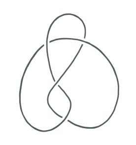
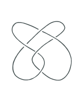
Figure 1: The hyperbolic knots known as the figure-eight knot ($\bm{4}_{1}$), on the left side, and the three-twist knot ($\bm{5}_{2}$), on the right side.

Throughout this work, we look at two concrete examples of hyperbolic knots, which allow us to perform explicit and detailed calculations to provide support to and give insight into our claims. These are the figure-eight and the three-twist knots.

Example 2.1.

The figure-eight knot, also denoted by $\bm{4}_{1}$, is shown on the left side of Fig. 1. Its classical $A$-polynomial can be written in symmetrized form as

$$A_{\bm{4}_{1}}(P,X)=P^{-1}+P-(X^{2}+X^{-2}-X-X^{-1}-2)\,.$$ (2.25)

The corresponding polynomial equation $A_{\bm{4}_{1}}(P,X)=0$ has only two distinct non-abelian branches. Explicitly, the geometric and conjugate branches are labeled as

$$\alpha=\rm{geom},\rm{conj}\,,$$ (2.26)

and they are described by

$$P^{(\rm{geom},\rm{conj})}=\frac{T(X)\pm(1-X^{2})\sqrt{\Delta(X)}}{2X^{2}}\,,$$ (2.27)

where we have introduced

$$T(X) =1-X-2X^{2}-X^{3}+X^{4}\,,$$ (2.28a)

$$\Delta(X) =1-2X-X^{2}-2X^{3}+X^{4}\,.$$ (2.28b)

Building on the results and conventions of ggm2 , the descendant $\hat{A}$-operator is given by

$$\hat{A}_{\bf{4}_{1}}(\hat{P},\hat{X},q^{m},q)=\sum_{j=0}^{2}C_{j}(\hat{X},q^{m},q)\hat{P}^{j}\,,$$ (2.29)

where $m$ takes values in ${\mathbb{Z}}$ and the coefficient functions $C_{j}(\hat{X},q^{m},q)$ are

$$C_{0}(\hat{X},q^{m},q)= q^{2+3m}\hat{X}^{2}(-1+q^{3+m}\hat{X}^{2})\,,$$ (2.30a)

$$C_{1}(\hat{X},q^{m},q)= -q^{m}(-1+q^{2+m}\hat{X}^{2})(1-q\hat{X}-q^{1+m}\hat{X}^{2}$$ (2.30b)

$$-q^{3+m}\hat{X}^{2}-q^{3+m}\hat{X}^{3}+q^{4+2m}\hat{X}^{4})\,,$$

$$C_{2}(\hat{X},q^{m},q)= q^{2}\hat{X}^{2}(-1+q^{1+m}\hat{X}^{2})\,.$$ (2.30c)

If we set $m=0$, symmetrize by multiplying by $\hat{P}^{-1}$, simplify a common factor $q^{2}\hat{X}^{2}$, and perform the change of variable $\hat{X}\rightarrow q^{-1}\hat{X}$, we obtain the conventional $\hat{A}$-operator of the figure-eight knot, that is,

$$\hat{A}_{\bf{4}_{1}}(\hat{P},\hat{X},q)=C_{0}(\hat{X},q)\hat{P}^{-1}+C_{1}(\hat{X},q)+C_{2}(\hat{X},q)\hat{P}\,,$$ (2.31)

where the coefficient functions $C_{j}(\hat{X},q)$ are

$$C_{0}(\hat{X},q)= q\hat{X}^{2}-1\,,$$ (2.32a)

$$C_{1}(\hat{X},q)= -(\hat{X}^{2}-1)(\hat{X}^{2}+\hat{X}^{-2}-\hat{X}-\hat{X}^{-1}-q-q^{-1})\,,$$ (2.32b)

$$C_{2}(\hat{X},q)= q^{-1}\hat{X}^{2}-1\,.$$ (2.32c)

Example 2.2.

The three-twist knot, also denoted by $\bm{5}_{2}$, is shown on the right side of Fig. 1. Its classical $A$-polynomial can be written in symmetrized form as

$$A_{\bm{5}_{2}}(P,X)= P^{-1}-(X^{-2}-X^{-1}+2X+2X^{2}-X^{3})$$ (2.33)

$$-(X^{-1}-2-2X+X^{3}-X^{4})P-X^{2}P^{2}\,.$$

The corresponding polynomial equation $A_{\bm{5}_{2}}(P,X)=0$ has three distinct non-abelian branches: the geometric branch, its conjugate, and a third, self-conjugate branch. We label them by

$$\alpha=\rm{geom},\rm{conj},\rm{\text{self}}\,.$$ (2.34)

Again, following ggm2 , the descendant $\hat{A}$-operator is given by

$$\hat{A}_{\bf{5}_{2}}(\hat{P},\hat{X},q^{m},q)=\sum_{j=0}^{3}C_{j}(\hat{X},q^{m},q)\hat{P}^{j}\,,$$ (2.35)

where $m$ takes values in ${\mathbb{Z}}$ and the coefficient functions $C_{j}(\hat{X},q^{m},q)$ are

$$C_{0}(\hat{X},q^{m},q)= -q^{2+m}\hat{X}^{2}(1-q^{2}\hat{X})(1+q^{2}\hat{X})(1-q^{5}\hat{X}^{2})\,,$$ (2.36a)

$$C_{1}(\hat{X},q^{m},q)= (1-q\hat{X})(1+q\hat{X})(1-q^{5}\hat{X}^{2})(1-q\hat{X}-q\hat{X}^{2}-q^{4}\hat{X}^{2}$$ (2.36b)

$$+q^{2+m}\hat{X}^{2}+q^{3+m}\hat{X}^{2}+q^{2}\hat{X}^{3}+q^{5}\hat{X}^{3}+q^{5}\hat{X}^{4}+q^{5+m}\hat{X}^{4}-q^{6}\hat{X}^{5})\,,$$

$$C_{2}(\hat{X},q^{m},q)= q\hat{X}(1-q^{2}\hat{X})(1+q^{2}\hat{X})(1-q\hat{X}^{2})(1-q^{2}\hat{X}-q^{2+m}\hat{X}-q^{2}\hat{X}^{2}-q^{5}\hat{X}^{2}$$ (2.36c)

$$+q^{4}\hat{X}^{3}+q^{7}\hat{X}^{3}-q^{5+m}\hat{X}^{3}-q^{6+m}\hat{X}^{3}+q^{7}\hat{X}^{4}-q^{9}\hat{X}^{5})\,,$$

$$C_{3}(\hat{X},q^{m},q)= q^{8+m}\hat{X}^{4}(1-q\hat{X})(1+q\hat{X})(1-q\hat{X}^{2})\,.$$ (2.36d)

If we set $m=0$, symmetrize by multiplying by $\hat{P}^{-2}$, and perform the change of variable $\hat{X}\rightarrow q^{-1}\hat{X}$, we obtain the conventional $\hat{A}$-operator of the three-twist knot, that is,

$$\hat{A}_{\bf{5}_{2}}(\hat{P},\hat{X},q)=C_{0}(\hat{X},q)\hat{P}^{-2}+C_{1}(\hat{X},q)\hat{P}^{-1}+C_{2}(\hat{X},q)+C_{3}(\hat{X},q)\hat{P}\,,$$ (2.37)

where we have defined

$$C_{0}(\hat{X},q)= -\hat{X}^{2}(1-q^{2}\hat{X}^{2})(1-q^{3}\hat{X}^{2})\,,$$ (2.38a)

$$C_{1}(\hat{X},q)= (1-\hat{X}^{2})(1-q^{3}\hat{X}^{2})(q^{2}\hat{X}^{3}-q^{2}\hat{X}^{2}-q\hat{X}^{5}$$ (2.38b)

$$+2q\hat{X}^{4}+q^{-1}\hat{X}^{3}+q\hat{X}^{2}-q^{-1}\hat{X}^{2}+\hat{X}^{2}-\hat{X}+1)\,,$$

$$C_{2}(\hat{X},q)= \hat{X}(1-q^{2}\hat{X}^{2})(1-q^{-1}\hat{X}^{2})(-q^{4}\hat{X}^{5}+q^{4}\hat{X}^{3}$$ (2.38c)

$$+q^{3}\hat{X}^{4}-q^{3}\hat{X}^{3}-q^{3}\hat{X}^{2}-q^{2}\hat{X}^{3}+q\hat{X}^{3}-2q\hat{X}-\hat{X}^{2}+1)\,,$$

$$C_{3}(\hat{X},q)= q^{4}\hat{X}^{4}(1-\hat{X}^{2})(1-q^{-1}\hat{X}^{2})\,.$$ (2.38d)

3 The structure of the wave function

In this section, we study the non-perturbative wave function $\chi_{{\cal K}}(u;\hbar)$ introduced in Section 2 by exploiting ideas from topological string theory. In particular, we propose various new conjectures on the structure of this wave function, which are motivated by similar results in the open version of the TS/ST correspondence kpamir ; mz-wv ; mz-wv2 ; szabolcs and by our detailed analysis of the examples presented in Section 4. In the following, we will not explicitly indicate the knot ${\cal K}$ to avoid the cluttering of notation.

3.1 General conjectures

Our first claim is that the WKB expansion in Eq. (2.17) can be resummed at all orders in $\hbar$ and order by order in $X={\rm e}^{2\pi{\mathsf{b}}u}$. Explicitly, for a fixed choice of $\alpha$, we have that

$$\chi^{(\alpha),\rm{WKB}}(u;\hbar)=\exp\left({{\rm i}\over\hbar}s^{(\alpha)}_{0}(x)+s^{(\alpha)}_{1}(x)+\phi^{(\alpha),\rm{WKB}}(X;q)\right)\,,$$ (3.39)

where $s^{(\alpha)}_{0,1}(x)$ are ${\mathbb{R}}$-polynomials in the variable $x=\log X$ and

$$\phi^{(\alpha),\rm{WKB}}(X;q)=\sum_{n\geq 1}a^{(\alpha)}_{n}(q)X^{n}+a^{(\alpha)}_{-n}(q)X^{-n}\,.$$ (3.40)

The coefficient functions $a^{(\alpha)}_{\pm n}(q)$ can be written as

$$a^{(\alpha)}_{\pm n}(q)={\hat{a}_{\pm n}^{(\alpha)}(q)\over n(q^{n}-1)q^{\sigma_{\alpha,\pm n}}}\,,\quad n\in{\mathbb{Z}}_{>0}\,,$$ (3.41)

where $\hat{a}^{(\alpha)}_{\pm n}(q)\in{\mathbb{Z}}[q]$ such that

$$\hat{a}^{(\rm{geom})}_{-n}(q)=0\,,\quad n\in{\mathbb{Z}}_{>0}\,,$$ (3.42)

and $\sigma_{\alpha,m}$ is a function of $m\in{\mathbb{Z}}_{\neq 0}$ which takes values in ${\mathbb{N}}$, depends on the choice of classical branch $\alpha$, and satisfies

$$\sigma_{{\rm geom},m}=0\,,\quad\sigma_{\alpha,-|m|}=0\,\quad\forall\alpha\,.$$ (3.43)

Note that we use the same notation for the perturbative WKB series in Eq. (2.17) and its resummation in terms of $q$ in Eq. (3.39). However, in the rest of this paper, we will always refer to the resummed version of $\chi^{(\alpha),\rm{WKB}}(u;\hbar)$ as in Eq. (3.39). In fact, there is additional structure in the resummed perturbative wave function. Our second claim is that $\phi^{(\alpha),\rm{WKB}}(X;q)$ has an integrality/multicovering-type structure. Namely, for a fixed choice of $\alpha$, we have that

$$\phi^{(\alpha),\rm{WKB}}(X;q)=\sum_{k,s\geq 1}{D^{(\alpha)}_{s}(q^{k})\over k(q^{k}-1)q^{k\sigma_{\alpha,s}}}X^{sk}+{D^{(\alpha)}_{-s}(q^{k})\over k(q^{k}-1)q^{k\sigma_{\alpha,-s}}}X^{-sk}\,,$$ (3.44)

where $D^{(\alpha)}_{\pm s}(q)\in{\mathbb{Z}}[q]$. Equivalently, we can write the coefficient functions from Eq. (3.40) as

$$a^{(\alpha)}_{\pm n}(q)=\sum_{k|n}{D^{(\alpha)}_{\pm{n\over k}}(q^{k})\over k(q^{k}-1)q^{k\sigma_{\alpha,\pm{n\over k}}}}\,,\quad n\in{\mathbb{Z}}_{>0}\,,$$ (3.45)

where the sum runs over all positive integer divisors of $n$. Since the following discussion holds for all non-abelian choices of the classical branch, let us now drop the explicit dependence on $\alpha$ to simplify the notation and introduce

$${\tilde{D}}_{\pm s}(q)={D_{\pm s}(q)\over(q-1)q^{\sigma_{\pm s}}}\,,\quad s\in{\mathbb{Z}}_{>0}\,.$$ (3.46)

As a consequence of Eq. (3.44), we can write

$$\exp\left(\phi^{\rm WKB}(X;q)\right)= \exp\left(\sum_{k,s\geq 1}{1\over k}{\tilde{D}}_{s}(q^{k})X^{sk}\right)\exp\left(\sum_{k,s\geq 1}{1\over k}{\tilde{D}}_{-s}(q^{k})X^{-sk}\right)$$ (3.47)

$$= {\rm Exp}_{X,q}\left(\sum_{s\geq 1}{\tilde{D}}_{s}(q)X^{s}\right){\rm Exp}_{X,q}\left(\sum_{s\geq 1}{\tilde{D}}_{-s}(q)X^{-s}\right)\,,$$

where ${\rm Exp}_{X,q}$ is the plethystic exponential in the variables $X,q$. See, e.g., lm-pv . It follows that we can extract the functions ${\tilde{D}}_{\pm s}(q)$ by applying the plethystic logarithm in the same two variables, which we denote by ${\rm Log}_{X,q}$, to both sides of Eq. (3.47). Specifically, we find that

$$\sum_{s\geq 1}{\tilde{D}}_{\pm s}(q)X^{\pm s}={\rm Log}_{X,q}\left(\exp\left(\sum_{n\geq 1}a_{\pm n}(q)X^{\pm n}\right)\right)=\sum_{k,n\geq 1}{\mu(k)\over k}a_{\pm n}(q^{k})X^{\pm nk}\,,$$ (3.48)

where $\mu(k)$ is the Möbius function, which leads to the closed formula

$${\tilde{D}}_{\pm s}(q)=\sum_{k|s}{\mu(k)\over k}a_{\pm{s\over k}}(q^{k})\,,\quad s\in{\mathbb{Z}}_{>0}\,.$$ (3.49)

Note that this is the formal inverse of Eq. (3.45), which can be equivalently written as

$$a_{\pm n}(q)=\sum_{k|n}{1\over k}{\tilde{D}}_{\pm{n\over k}}(q^{k})\,,\quad n\in{\mathbb{Z}}_{>0}\,.$$ (3.50)

We comment that, in both examples of the figure-eight and the three-twist knots studied in Section 4, we have precise expressions for $\sigma_{\alpha,m}$ for all choices of $\alpha\neq\rm{geom}$, which are given in Eqs. (4.140), (4.160), and (4.161). Moreover, our statements above simplify notably in the particular case of the geometric branch, whose function $\phi^{(\rm{geom}),\rm{WKB}}(X;q)$ has a series expansion including only the positive powers of $X$ and whose coefficients $a^{(\rm{geom})}_{n}(q)$ have a trivial factor of $q^{\sigma_{{\rm geom},n}}=1$ in the denominator.

Let us explain how our conjectures originate from insights from the TS/ST correspondence. See mmrev for a review and further references. In the context of the TS/ST correspondence, the analog of the AJ conjecture for the wave function in Eq. (2.20) is given by the quantization of the mirror curve to a toric Calabi–Yau threefold, which defines a spectral problem. Its wave function can be computed in the WKB approximation as a formal power series in $\hbar$. It was noted in kpamir ; mz-wv that this $\hbar$-expansion can be suitably resummed, producing the same picture that we have described in our claims above. This structure is similar to the one appearing in perturbative open topological string theory ov ; lmv , but it is slightly less constrained. Specifically, one has the structure of ov but not the more detailed substructure found in lmv . The integrality property in Eq. (3.44) defines what is called an admissible series in ks and is found in other examples like, e.g., in as .

We can now ask how the resummed, perturbative partition functions in Eq. (3.39) relate to the exact partition function $\chi(u;\hbar)$ described in Section 2. It follows both from physical arguments bdp and from explicit calculations gk-qseries ; dimofte-levelk ; ggm2 that the exact wave function can be decomposed as

$$\chi(u;\hbar)=\sum_{\alpha}\mathsf{C}_{\alpha}\,{\cal S}^{(\alpha)}(X;q){\cal S}^{(\alpha)}(X_{D};q_{D})\,,$$ (3.51)

where the sum runs over the different branches of the classical $A$-polynomial labeled by $\alpha$, $\mathsf{C}_{\alpha}$ is an appropriate complex constant, and ${\cal S}^{(\alpha)}(X;q)$ is known as holomorphic block. Since the holomorphic block must reproduce the perturbative expansion of the wave function, it can be identified with the resummed WKB series in Eq. (3.39), that is,

$${\cal S}^{(\alpha)}(X;q)=\exp\left(\frac{{\rm i}}{\hbar}s^{(\alpha)}_{0}(x)+s^{(\alpha)}_{1}(x)+\phi^{(\alpha),\rm{WKB}}(X;q)\right)\,.$$ (3.52)

Therefore, our conjecture in Eq. (3.44) implies that holomorphic blocks in complex CS theory have the stated integrality/multicovering property, i.e., they are admissible series in the Kontsevich–Soibelman sense. This could have been anticipated from the relation between holomorphic blocks and open topological string partition functions in some examples bdp . Indeed, we will show in Section 4 that, starting from the known closed expression for the holomorphic and antiholomorphic blocks, we can successfully verify the integrality structure of Eq. (3.44) in the examples of the figure-eight and the three-twist knots for all choices of the saddle connection $\alpha$.

Let us comment that the structure in Eqs. (3.51), (3.52) is again similar to what has been found in the open TS/ST correspondence kpamir ; mz-wv ; mz-wv2 ; szabolcs ; fgrassi : the exact wave functions are given by sums of products of the resummed WKB wave functions and their duals. As we mentioned in Section 1, a structure similar to the one in Eq. (3.40) has already been conjectured in ekholm , where the resummed WKB expansion is obtained by solving directly the quantized $A$-polynomial equation. The approach of ekholm does not appeal to the decomposition into holomorphic blocks, and our explicit results for the resummation of the WKB expansion in the case of, e.g., the figure-eight knot in Section 4 appear to be different from those in ekholm .

3.2 Cancellation of singularities

Again, we hide the explicit dependence on the classical solution $\alpha$ to simplify the notation. Here and in the rest of this work, we will only re-introduce it when necessary. Recall that the exact wave function $\chi(u;\hbar)$ is well-defined for $\hbar>0$. In particular, it is well-defined for

$$\hbar=2\pi{P\over Q}\,,$$ (3.53)

where $P,Q$ are coprime positive integers. We will refer to values of $\hbar$ of the form in Eq. (3.53) as rational values. On the other hand, due to the conjectured integrality structure in Eq. (3.44), $\phi^{\rm WKB}(X;q)$ is singular for these values of $\hbar$ precisely, thus implying that the singularities have to cancel in the sum

$$\phi^{\rm WKB}(X;q)+\phi^{\rm WKB}(X_{D};q_{D})\,,$$ (3.54)

which appears in the formula for $\chi(u;\hbar)$ in Eq. (3.51). This leads to non-trivial constraints on the coefficients $\hat{a}_{\pm n}(q)$ in Eq. (3.41). This type of cancellation of singularities played a major role in the understanding of the ABJM matrix model hmo2 and the TS/ST correspondence km ; ghm ; wzh .

We will now study how this cancellation occurs in the exact wave function $\chi(u;\hbar)$ as given in Eq. (3.51), and, in Section 3.3, we will compute the finite, well-defined piece which is left from the cancellation and constitutes the sum in Eq. (3.54). Moreover, as we will see following szabolcs in Section 3.4, it is possible to compute this finite part by using only the information contained in the quantum operator $\hat{A}(\hat{P},\hat{X},q)$. We take

$$q={\rm e}^{{\rm i}\hbar}={\rm e}^{2\pi{\rm i}{P\over Q}}\,,\quad P,Q\in{\mathbb{Z}}_{>0}\;\;\text{coprime}\,,$$ (3.55)

and, substituting into Eq. (3.40), we find that the possible singularities of $\phi^{\rm WKB}(X;q)$ occur in $a_{\pm n}(q)$ when $n=sQ$ and $s\in{\mathbb{Z}}_{>0}$. For these values of $n$, the coefficient functions $a_{\pm n}(q)$ in Eq. (3.41) become

$$a_{\pm sQ}\left(q\right)=\frac{\hat{a}_{\pm sQ}\left(q\right)}{sQ(q^{sQ}-1)q^{\sigma_{\pm sQ}}}\,.$$ (3.56)

Similarly, considering the dual variable

$$q_{D}={\rm e}^{{4\pi^{2}\over\hbar}}={\rm e}^{2\pi{\rm i}{Q\over P}}\,,$$ (3.57)

the possible singularities of the dual function $\phi_{\rm WKB}(X_{D};q_{D})$ occur in $a_{\pm n}(q_{D})$ when $n=sP$ and $s\in{\mathbb{Z}}_{>0}$. Indeed, the coefficient functions $a_{\pm n}(q_{D})$ in Eq. (3.41) become

$$a_{\pm sP}\left(q_{D}\right)=\frac{\hat{a}_{\pm sP}\left(q_{D}\right)}{sP(q_{D}^{sP}-1)q_{D}^{\sigma_{\pm sP}}}\,.$$ (3.58)

Let us now introduce

$$q_{\epsilon}={\rm e}^{{\rm i}\hbar_{\epsilon}}\,,\quad q_{\epsilon,D}={\rm e}^{{4\pi^{2}{\rm i}\over\hbar_{\epsilon}}}\,,\quad\hbar_{\epsilon}=2\pi{P\over Q}+\epsilon\,,\quad 0<\epsilon\ll 1\,,$$ (3.59)

and consider the limit $\epsilon\rightarrow 0$. As detailed in Appendix A, Eqs. (3.56), (3.58) produce the NLO $\epsilon$-expansions

$$a_{\pm sQ}\left(q_{\epsilon}\right) =\left(-\frac{{\rm i}}{(sQ)^{2}\epsilon}-\frac{1}{2sQ}+\frac{1}{(sQ)^{2}}q\frac{\partial}{\partial q}\right)\frac{\hat{a}_{\pm sQ}(q)}{q^{\sigma_{\pm sQ}}}+{\cal O}(\epsilon)\,,$$ (3.60a)

$$a_{\pm sP}\left(q_{\epsilon,D}\right) =\left(\frac{{\rm i}}{(sQ)^{2}\epsilon}+\frac{1}{sP}\left(\frac{{\rm i}}{2\pi sQ}-{1\over 2}\right)+\frac{1}{(sP)^{2}}q_{D}\frac{\partial}{\partial q_{D}}\right)\frac{\hat{a}_{\pm sP}(q_{D})}{q_{D}^{\sigma_{\pm sP}}}+{\cal O}(\epsilon)\,.$$ (3.60b)

We then require the cancellation of the $\epsilon$-poles in Eqs. (3.60a), (3.60b), which yields the relation

$$\hat{a}_{\pm sQ}\left({\rm e}^{2\pi{\rm i}{P\over Q}}\right){\rm e}^{-2\pi{\rm i}{P\over Q}\sigma_{\pm sQ}}=\hat{a}_{\pm sP}\left({\rm e}^{2\pi{\rm i}{Q\over P}}\right){\rm e}^{-2\pi{\rm i}{Q\over P}\sigma_{\pm sP}}\,,$$ (3.61)

for all $s,P,Q\in{\mathbb{Z}}_{>0}$ with $P,Q$ coprime. We remark that, for the geometric branch, the formula in Eq. (3.61) assumes the simplified form

$$\hat{a}^{(\rm{geom})}_{sQ}\left({\rm e}^{2\pi{\rm i}{P\over Q}}\right)=\hat{a}^{(\rm{geom})}_{sP}\left({\rm e}^{2\pi{\rm i}{Q\over P}}\right)\,,$$ (3.62)

where again $s,P,Q\in{\mathbb{Z}}_{>0}$ with $P,Q$ coprime.

Let us now prove that the cancellation formula in Eq. (3.61) is indeed a consequence of the integrality structure presented in Eq. (3.44). More precisely, Eqs. (3.41), (3.45) imply that

$$\hat{a}_{n}(q)q^{-\sigma_{n}}=\sum_{k|n}kD_{k}\left(q^{n\over k}\right)q^{-{n\over k}\sigma_{k}}\sum_{j=0}^{k-1}q^{{n\over k}j}\,,$$ (3.63)

and, after substituting $n=sQ$ and $q={\rm e}^{2\pi{\rm i}{P\over Q}}$ with $s,P,Q$ as above, we obtain

$$\hat{a}_{sQ}\left({\rm e}^{2\pi{\rm i}{P\over Q}}\right){\rm e}^{-2\pi{\rm i}{P\over Q}\sigma_{sQ}}=\sum_{k|sQ}kD_{k}\left({\rm e}^{2\pi{\rm i}\frac{sP}{k}}\right){\rm e}^{-2\pi{\rm i}\frac{sP}{k}\sigma_{k}}\sum_{j=0}^{k-1}{\rm e}^{2\pi{\rm i}\frac{sP}{k}j}\,.$$ (3.64)

Since the sum over $j$ on the RHS is non-zero if and only if $k|s$, Eq. (3.64) gives

$$\hat{a}_{sQ}\left({\rm e}^{2\pi{\rm i}{P\over Q}}\right){\rm e}^{-2\pi{\rm i}{P\over Q}\sigma_{sQ}}=\sum_{k|s}k^{2}D_{k}(1)=c_{s}\in{\mathbb{Z}}\,,\quad s\in{\mathbb{Z}}_{>0}\,,$$ (3.65)

which is independent of the choice of $P,Q\in{\mathbb{Z}}_{>0}$ coprime, thus proving the cancellation identity in Eq. (3.61). We note that the case of $\hat{a}_{-n}(q)$ is handled analogously, yielding the same result. In particular, recalling that $\sigma_{-n}=0$, $n\in{\mathbb{Z}}_{>0}$, it defines the sequence of integers

$$\hat{a}_{-sQ}\left({\rm e}^{2\pi{\rm i}{P\over Q}}\right)=\sum_{k|s}k^{2}D_{-k}(1)=c_{-s}\in{\mathbb{Z}}\,,\quad s\in{\mathbb{Z}}_{>0}\,.$$ (3.66)

Finally, applying the Möbius inversion formula for arithmetic functions, we deduce that

$$D_{\pm s}(1)={1\over s^{2}}\sum_{k|s}\mu(k)c_{\pm{s\over k}}\,,\quad s\in{\mathbb{Z}}_{>0}\,,$$ (3.67)

where $\mu(k)$ is the Möbius function. As we will see, the construction presented here is experimentally verified for the knots ${\bf 4}_{1}$ and ${\bf 5}_{2}$ in Section 4.

3.3 The wave function in the rational case, I

We will now apply the results obtained in Section 3.2 to derive explicitly the exact wave function $\chi(u;\hbar)$ in Eq. (3.51) as a power series in $X,X^{-1}$ for rational values of $\hbar$. Let us start from the holomorphic components $\phi^{(\alpha),{\rm WKB}}(X;q)$ and fix $\hbar$ as in Eq. (3.53), that is,

$$q={\rm e}^{{\rm i}\hbar}={\rm e}^{2\pi{\rm i}{P\over Q}}\,,\quad P,Q\in{\mathbb{Z}}_{>0}\;\;\text{coprime}\,.$$ (3.68)

As before, we drop the label $\alpha$ for simplicity and we intend the following discussion to hold for each choice of the classical branch independently. The singular terms come from the values $n=sQ$ for $s\in{\mathbb{Z}}_{>0}$, while choosing $n=sQ+k$ with $1\leq k\leq Q-1$ produces only regular terms. Specifically, the terms involving singularities are obtained by substituting Eq. (3.60a) into Eq. (3.40) and contain the non-singular contributions

$$\sum_{s\geq 1}\left(-{1\over 2}+{1\over sQ}q{\partial\over\partial q}\right)\frac{\hat{a}_{\pm sQ}(q)}{sQq^{\sigma_{\pm sQ}}}X^{\pm sQ}\,.$$ (3.69)

The regular terms associated with $n\neq sQ$ are instead

$$\sum_{k=1}^{Q-1}\frac{1}{q^{k}-1}\sum_{s\geq 0}{\hat{a}_{\pm(sQ+k)}(q)\over(sQ+k)q^{\sigma_{\pm(sQ+k)}}}X^{\pm(sQ+k)}\,,$$ (3.70)

where we have used that $q^{sQ+k}=q^{k}$. Thus, the sum of the quantities in Eqs. (3.69), (3.70) is the finite part of $\phi^{\rm WKB}(X;q)$ evaluated at the rational point in Eq. (3.53). It is convenient to introduce the functions

$$\varphi^{(+)}_{Q}(X) =\sum_{s\geq 1}{\hat{a}_{sQ}(q)\over sQq^{\sigma_{sQ}}}X^{sQ}\,,$$ (3.71a)

$$\varphi^{(-)}_{Q}(X) =\sum_{s\geq 1}{\hat{a}_{-sQ}(q)\over(-sQ)q^{sQ+\sigma_{-sQ}}}X^{-sQ}\,,$$ (3.71b)

$$\varphi^{(+)}_{k}(X) =\sum_{s\geq 0}{\hat{a}_{sQ+k}(q)\over(sQ+k)q^{\sigma_{sQ+k}}}X^{sQ+k}\,,\quad k=1,\dots,Q-1\,,$$ (3.71c)

$$\varphi^{(-)}_{k}(X) =\sum_{s\geq 0}{\hat{a}_{-(sQ+k)}(q)\over-(sQ+k)q^{sQ+k+\sigma_{-(sQ+k)}}}X^{-(sQ+k)}\,,\quad k=1,\dots,Q-1\,,$$ (3.71d)

where we hide the dependence on $q$ to simplify the notation. Moreover, we define

$$\varphi_{Q}(X) =\varphi^{(+)}_{Q}(X)+\varphi^{(-)}_{Q}(X)\,,$$ (3.72a)

$$\varphi_{k}(X) =\varphi^{(+)}_{k}(X)-q^{k}\varphi^{(-)}_{k}(X)\,,\quad k=1,\dots,Q-1\,.$$ (3.72b)

Putting Eqs. (3.69), (3.70) together and suitably identifying the functions just introduced in Eq. (3.72), we can write the holomorphic block as

$$\phi^{\rm WKB}(X;q)=-{1\over 2}\varphi_{Q}(X)+q{\partial\over\partial q}\int_{0}^{X}\varphi_{Q}(X^{\prime}){{\rm d}X^{\prime}\over X^{\prime}}+\sum_{k=1}^{Q-1}{\varphi_{k}(X)\over q^{k}-1}\,.$$ (3.73)

Let us now consider the antiholomorphic component $\phi^{\rm WKB}(X_{D};q_{D})$ and fix $\hbar$ as above. The derivation in this case is very similar to the previous one, but the novelty is the appearance of $\log X$ terms, which originate from the $\epsilon$-expansion of the dual variable

$$X_{D}=X^{2\pi\over\hbar}=X^{Q\over P}\,.$$ (3.74)

Let us add a small positive term $\epsilon$ to the rational value of $\hbar$ as in Eq. (3.59). Then, we consider the limit $\epsilon\rightarrow 0$ and find that

$$X_{\epsilon,D}=X^{2\pi\over\hbar_{\epsilon}}=X^{{Q\over P}{1\over 1+{\epsilon\over 2\pi}{Q\over P}}}=X^{Q\over P}\left(1-{Q^{2}\over 2\pi P^{2}}\epsilon\log X+{\cal O}(\epsilon^{2})\right)\,.$$ (3.75)

As described before, the singular terms come from the values $n=sP$ for $s\in{\mathbb{Z}}_{>0}$, while choosing $n=sP+k$ with $1\leq k\leq P-1$ produces only regular terms. Specifically, the terms involving singularities are obtained by substituting Eqs. (3.60b), (3.75) into the Eq. (3.40) and contain the non-singular contributions

$$\sum_{s\geq 1}\left(\frac{{\rm i}}{2\pi sQ}-{1\over 2}+{1\over sP}q_{D}{\partial\over\partial q_{D}}\mp\frac{{\rm i}}{2\pi}\log X\right)\frac{\hat{a}_{\pm sP}(q_{D})}{sPq_{D}^{\sigma_{\pm sP}}}X^{\pm sQ}\,.$$ (3.76)

The regular terms associated with $n\neq sP$ are instead

$$\sum_{k=1}^{P-1}\frac{1}{q_{D}^{k}-1}\sum_{s\geq 0}{\hat{a}_{\pm(sP+k)}(q_{D})\over(sP+k)q_{D}^{\sigma_{\pm(sP+k)}}}X^{\pm(sP+k){Q\over P}}\,,$$ (3.77)

where we have used that $q_{D}={\rm e}^{2\pi{Q\over P}}$ and thus $q_{D}^{sP+k}=q_{D}^{k}$. Therefore, the sum of the quantities in Eqs. (3.76), (3.77) is the finite part of the function $\phi^{\rm WKB}(X_{D};q_{D})$ evaluated at the rational point in Eq. (3.53). As for the holomorphic block, we introduce the functions

$$\widetilde{\varphi}^{(+)}_{P}(X_{D}) =\sum_{s\geq 1}{\hat{a}_{sP}(q_{D})\over sPq_{D}^{\sigma_{sP}}}X_{D}^{sP}\,,$$ (3.78a)

$$\widetilde{\varphi}^{(-)}_{P}(X_{D}) =\sum_{s\geq 1}{\hat{a}_{-sP}(q_{D})\over-(sP)q_{D}^{sP+\sigma_{-sP}}}X_{D}^{-sP}\,,$$ (3.78b)

$$\widetilde{\varphi}^{(+)}_{k}(X_{D}) =\sum_{s\geq 0}{\hat{a}_{sP+k}(q_{D})\over(sP+k)q_{D}^{\sigma_{sP+k}}}X_{D}^{sP+k}\,,\quad k=1,\dots,P-1\,,$$ (3.78c)

$$\widetilde{\varphi}^{(-)}_{k}(X_{D}) =\sum_{s\geq 0}{\hat{a}_{-(sP+k)}(q_{D})\over-(sP+k)q_{D}^{sP+k+\sigma_{-(sP+k)}}}X_{D}^{-(sP+k)}\,,\quad k=1,\dots,P-1\,,$$ (3.78d)

where we hide the dependence on $q_{D}$ to simplify the notation. Moreover, we define

$$\widetilde{\varphi}_{P}(X_{D}) =\widetilde{\varphi}^{(+)}_{P}(X_{D})+\widetilde{\varphi}^{(-)}_{P}(X_{D})\,,$$ (3.79a)

$$\widetilde{\varphi}_{k}(X_{D}) =\widetilde{\varphi}^{(+)}_{k}(X_{D})-q_{D}^{k}\widetilde{\varphi}^{(-)}_{k}(X_{D})\,,\quad k=1,\dots,Q-1\,.$$ (3.79b)

Putting Eqs. (3.76), (3.77) together and suitably identifying the functions just introduced in Eq. (3.79), we can now write the antiholomorphic block as

$$\phi^{\rm WKB}(X_{D};q_{D})= -\left({1\over 2}+{{\rm i}\over 2\pi}\log X\right)\widetilde{\varphi}_{P}(X_{D})$$ (3.80)

$$+\left({{\rm i}P\over 2\pi Q}+q_{D}{\partial\over\partial q_{D}}\right)\int_{0}^{X_{D}}\widetilde{\varphi}_{P}(X_{D}^{\prime}){{\rm d}X_{D}^{\prime}\over X_{D}^{\prime}}+\sum_{k=1}^{P-1}{\widetilde{\varphi}_{k}(X_{D})\over q_{D}^{k}-1}\,.$$

Finally, we observe that

$$\widetilde{\varphi}^{(+)}_{P}(X_{D})={Q\over P}\varphi^{(+)}_{Q}(X)\,,\quad\widetilde{\varphi}^{(-)}_{P}(X_{D})={Q\over P}q^{sQ\left(1-\frac{Q}{P}\right)}\varphi^{(-)}_{Q}(X)\,,$$ (3.81)

as a direct consequence of the cancellation symmetry in Eq. (3.61). Therefore, after summing Eqs. (3.73), (3.80) and using the relations in Eq. (3.81), we obtain the expression

$$\phi^{\rm WKB}(X;q)+\phi^{\rm WKB}(X_{D};q_{D})= \left(-{1\over 2}-{Q\over 2P}-{{\rm i}Q\over 2\pi P}\log X\right)\varphi_{Q}(X)$$ (3.82)

$$+\left({{\rm i}Q\over 2\pi P}+2q{\partial\over\partial q}\right)\int_{0}^{X}\varphi_{Q}(X^{\prime}){{\rm d}X^{\prime}\over X^{\prime}}$$

$$+sQ\left(1-\frac{Q}{P}\right)\int_{0}^{X}\varphi^{(-)}_{Q}(X^{\prime}){{\rm d}X^{\prime}\over X^{\prime}}$$

$$+\sum_{k=1}^{Q-1}{\varphi_{k}(X)\over q^{k}-1}+\sum_{k=1}^{P-1}{\widetilde{\varphi}_{k}(X^{Q\over P})\over q^{k{Q^{2}\over P^{2}}}-1}\,.$$

Moreover, the power series defined in Eqs. (3.72), (3.79), which dictate the formula for the exact wave function at rational points following Eq. (3.82), are determined by the function

$$\Upsilon(X)=\Upsilon^{(+)}(X)+\Upsilon^{(-)}(X)=\sum_{n\geq 1}{\hat{a}_{n}(q)\over nq^{\sigma_{n}}}X^{n}+\sum_{n\geq 1}{\hat{a}_{-n}(q)\over(-n)q^{n+\sigma_{-n}}}X^{-n}\,,$$ (3.83)

where, again, we hide the dependence on $q$ to simplify the notation. Indeed, we can write

$$\varphi_{Q}(X) ={1\over Q}\sum_{m=0}^{Q-1}\Upsilon(q^{m}X)\,,$$ (3.84a)

$$\varphi^{(\pm)}_{k}(X) ={1\over Q}\sum_{m=0}^{Q-1}q^{\mp mk}\,\Upsilon^{(\pm)}(q^{m}X,q)\,,\quad k=1,\dots,Q-1\,,$$ (3.84b)

and similarly

$$\widetilde{\varphi}_{P}(X_{D}) ={1\over P}\sum_{m=0}^{P-1}\Upsilon(q_{D}^{m}X_{D})\,,$$ (3.85a)

$$\widetilde{\varphi}^{(\pm)}_{k}(X_{D}) ={1\over P}\sum_{m=0}^{P-1}q_{D}^{\mp mk}\,\Upsilon^{(\pm)}(q_{D}^{m}X_{D})\,,\quad k=1,\dots,P-1\,.$$ (3.85b)

Let us stress that the derivation we have presented here implies a fixed choice of the classical branch. Indeed, the functions $\Upsilon(X),\varphi_{Q}(X),\varphi_{k}(X),\widetilde{\varphi}_{P}(X_{D}),\widetilde{\varphi}_{k}(X_{D})$ are implicitly dependent on the label $\alpha$. We note that, applying Eqs. (3.65), (3.66), we can simply read off the integer coefficients $c_{\pm s}$, $s\in{\mathbb{Z}}_{>0}$, from the function $\varphi_{Q}(X)$. Namely, we have that

$$\varphi_{Q}(X)=\sum_{s\geq 1}{c_{s}\over sQ}X^{sQ}-{c_{-s}\over sQ}X^{-sQ}\,,$$ (3.86)

after substituting $q^{sQ}=1$. In Appendix B, we describe an alternative way of computing the integer sequences $\{c_{\pm s}\}$, $s\in{\mathbb{Z}}_{>0}$ using Eq. (3.82). We will show in Section 4 that, starting from the known closed expression for the holomorphic and antiholomorphic blocks, we can successfully compute the integer coefficients for both series in $X,X^{-1}$ and all choices of the saddle connection $\alpha$ in the examples of the figure-eight and the three-twist knots.

3.4 The wave function in the rational case, II

In Section 3.3, we showed that the exact wave function $\chi(u;\hbar)$ in Eq. (3.51) at rational values of $\hbar$ is determined by the functions $\Upsilon^{(\alpha)}(X)$, defined in Eq. (3.83), and their derivatives with respect to $q$, up to the constants $\mathsf{C}_{\alpha}$ and the exponential prefactors containing $s^{(\alpha)}_{0,1}(x)$. We will now prove that the functions $\Upsilon^{(\alpha)}(X)$ can be obtained by solving directly the quantum $A$-polynomial in closed form. We will focus on $q$-difference equations of order two and three. These are the relevant cases for the examples studied in Section 4. The matrix formalism presented below was used in szabolcs for a second-order $q$-difference equation in the context of quantum mirror curves.

3.4.1 Solving a second-order $q$-difference equation

Recall that, for each choice of $\alpha$, the resummed perturbative wave function $\chi^{(\alpha),\rm{WKB}}(u;\hbar)$ is given in Eq. (3.39). Equivalently, we write

$$\chi^{(\alpha),\rm{WKB}}(u;\hbar)={\rm e}^{\frac{{\rm i}}{\hbar}s^{(\alpha)}_{0}(x)+s^{(\alpha)}_{1}(x)}\Psi^{(\alpha),\rm{WKB}}(X;q)\,,$$ (3.87)

where we have introduced the notation

$$\Psi^{(\alpha),\rm{WKB}}(X;q)=\exp\left(\phi^{(\alpha),\rm{WKB}}(X;q)\right)\,,$$ (3.88)

which will be useful in the following discussion. Let us assume that the corresponding quantum $A$-polynomial equation, that is,

$$\hat{A}(\hat{P},\hat{X},q)\chi^{(\alpha),\rm{WKB}}(u;\hbar)=0\,,$$ (3.89)

is of second order. After appropriately accounting for the correction due to the exponential prefactor containing the functions $s^{(\alpha)}_{0,1}(x)$ in Eq. (3.87), the $q$-difference equation above becomes

$$\Psi^{(\alpha),\rm{WKB}}(qX;q)+A(X)\Psi^{(\alpha),\rm{WKB}}(X;q)+B(X)\Psi^{(\alpha),\rm{WKB}}(q^{-1}X;q)=0\,,$$ (3.90)

where $A(X),B(X)$ are functions of $X$ and $q$. Let us observe that, due to the conjectural structure in Eqs. (3.40), (3.41), we have

$$\upsilon^{(\alpha)}(X)={\Psi^{(\alpha),\rm{WKB}}(qX;q)\over\Psi^{(\alpha),\rm{WKB}}(X;q)}=\exp\left(\Upsilon^{(\alpha)}(X)\right)\,,$$ (3.91)

and we can now write Eq. (3.90) in terms of the above function $\upsilon^{(\alpha)}(X)$ as

$$\upsilon(X)\upsilon(q^{-1}X)+A(X)\upsilon(q^{-1}X)+B(X)=0\,,$$ (3.92)

where we have dropped the label $\alpha$ from the notation for simplicity. Let us further assume that $\hbar$ is fixed as in Eq. (3.53), that is,

$$q={\rm e}^{{\rm i}\hbar}={\rm e}^{2\pi{\rm i}{P\over Q}}\,,\quad P,Q\in{\mathbb{Z}}_{>0}\;\;\text{coprime}\,,$$ (3.93)

and introduce the sequence of functions $\{\upsilon_{k}\}$, $k\in{\mathbb{Z}}_{\geq 0}$, of $X$ and $q$ defined by

$$\upsilon_{k}=\upsilon(q^{-k}X)\,.$$ (3.94)

They satisfy the system of equations

$$\upsilon_{k}\upsilon_{k+1}+A(q^{-k}X)\upsilon_{k+1}+B(q^{-k}X)=0\,,\quad 0\leq k\leq Q-1\,,$$ (3.95)

as a consequence of Eq. (3.92). We solve this system recursively, as follows. We define the sequences $\{a^{(k)}(X)\}$ and $\{b^{(k)}(X)\}$, $k\in{\mathbb{Z}}_{\geq 0}$, via the relations

$$a^{(1)}(X)=A(X),$$ (3.96a)

$$b^{(1)}(X)=B(X),$$ (3.96b)

$$\upsilon_{0}\upsilon_{1}\cdots\upsilon_{k}+a^{(k)}(X)\upsilon_{k}+b^{(k)}(X)=0\,,\quad k>1\,.$$ (3.96c)

If we multiply Eq. (3.96c) by $\upsilon_{k+1}$ and apply Eq. (3.95), we obtain a recursion relation which can be written in matrix form as

$$\begin{pmatrix}a^{(k+1)}(X)\\ b^{(k+1)}(X)\end{pmatrix}=\begin{pmatrix}-A(q^{-k}X)&1\\ -B(q^{-k}X)&0\end{pmatrix}\begin{pmatrix}a^{(k)}(X)\\ b^{(k)}(X)\end{pmatrix}\,,$$ (3.97)

and it can be solved as

$$\begin{pmatrix}a^{(Q)}(X)\\ b^{(Q)}(X)\end{pmatrix}={\mathcal{M}}_{Q}(X)\begin{pmatrix}-1\\ 0\end{pmatrix}\,.$$ (3.98)

Here, ${\mathcal{M}}_{Q}(X)$ is the matrix

$${\cal M}_{Q}(X)=\prod_{k=1}^{Q}\begin{pmatrix}-A(q^{k}X)&1\\ -B(q^{k}X)&0\end{pmatrix}=\begin{pmatrix}{\cal M}_{11}(X)&{\cal M}_{12}(X)\\ {\cal M}_{21}(X)&{\cal M}_{22}(X)\end{pmatrix}\,,$$ (3.99)

where the product is ordered from left to right as $k$ increases. Recalling that $q^{Q}=1$, we obtain

$${\mathcal{M}}_{Q}(q^{-1}X) =\begin{pmatrix}-A(X)&1\\ -B(X)&0\end{pmatrix}{\mathcal{M}}_{Q}(X)\begin{pmatrix}-A(X)&1\\ -B(X)&0\end{pmatrix}^{-1}$$ (3.100)

$$=\begin{pmatrix}{\cal M}_{22}-A{\cal M}_{12}&\frac{A}{B}\left({\cal M}_{11}+A{\cal M}_{12}\right)-\frac{1}{B}\left({\cal M}_{21}+A{\cal M}_{22}\right)\\ -B{\cal M}_{12}&{\cal M}_{11}+A{\cal M}_{12}\end{pmatrix}\,,$$

where we have removed the explicit dependence on $X$ for compactness. Following Eqs. (3.98), (3.100), we find that

$$\begin{pmatrix}a^{(Q)}(q^{-1}X)\\ b^{(Q)}(q^{-1}X)\end{pmatrix}=\begin{pmatrix}{-\mathcal{M}}_{22}(X)+A(X){\mathcal{M}}_{12}(X)\\ B(X){\mathcal{M}}_{12}(X)\end{pmatrix}\,.$$ (3.101)

Let us now define the function

$$\Pi\upsilon=\upsilon_{0}\upsilon_{1}\cdots\upsilon_{Q-1}\,,$$ (3.102)

which is invariant under $q$-shifts. We consider Eq. (3.96c) for $k=Q$ and, shifting $X$ into $q^{-1}X$, we produce the system

$$\begin{cases}\upsilon_{0}(\Pi\upsilon+a^{(Q)}(X))+b^{(Q)}(X)=0\,,\\ \upsilon_{1}(\Pi\upsilon+a^{(Q)}(q^{-1}X))+b^{(Q)}(q^{-1}X)=0\,.\end{cases}$$ (3.103)

By substituting the expressions for $a^{(Q)}(X),a^{(Q)}(q^{-1}X)$ and $b^{(Q)}(X),b^{(Q)}(q^{-1}X)$ in terms of the entries of the original matrix $\mathcal{M}_{Q}(X)$ in Eqs. (3.98), (3.101) and then using Eq. (3.95) with $k=0$, we can rewrite the system above as

$$\begin{cases}\upsilon_{0}(\Pi\upsilon-{\mathcal{M}}_{11}(X))-{\mathcal{M}}_{21}(X)=0\,,\\ \Pi\upsilon-{\mathcal{M}}_{22}(X)-\upsilon_{0}{\mathcal{M}}_{12}(X)=0\,,\end{cases}$$ (3.104)

or, equivalently, in the matrix form

$$\begin{pmatrix}{\mathcal{M}}_{11}(X)-\Pi\upsilon&{\mathcal{M}}_{21}(X)\\ {\mathcal{M}}_{12}(X)&{\mathcal{M}}_{22}(X)-\Pi\upsilon\end{pmatrix}\begin{pmatrix}\upsilon_{0}\\ 1\end{pmatrix}=\begin{pmatrix}0\\ 0\end{pmatrix}\,.$$ (3.105)

It follows straightforwardly that $\Pi\upsilon$ is an eigenvalue of the transpose matrix $\mathcal{M}_{Q}(X)^{\rm T}$ with eigenvector $(\upsilon_{0},1)^{\rm T}$. Specifically, we have that

$$\Pi\upsilon=\frac{{\rm tr}{\mathcal{M}_{Q}}(X)\pm\sqrt{\Delta_{Q}(X)}}{2}\,,$$ (3.106)

where we have introduced

$$\Delta_{Q}(X)=({\rm tr}{\mathcal{M}_{Q}}(X))^{2}-4\,\,{\rm det}{\mathcal{M}_{Q}}(X)\,,$$ (3.107)

while ${\rm det}{\mathcal{M}_{Q}}(X)$ and ${\rm tr}{\mathcal{M}_{Q}}(X)$ denote the trace and determinant of the matrix, respectively. Note that, following Eq. (3.99), both ${\rm det}{\mathcal{M}_{Q}}(X)$ and ${\rm tr}{\mathcal{M}_{Q}}(X)$ are invariant under $q$-shifts and so depend on $X$ through $X^{Q}$. The function $\upsilon_{0}$ can be found, for example, using the second line of Eq. (3.104), yielding

$$\upsilon_{0}=\frac{\Pi v-{\mathcal{M}}_{22}(X)}{{\mathcal{M}}_{12}(X)}=\frac{{\mathcal{M}}_{11}(X)-{\mathcal{M}}_{22}(X)\pm\sqrt{\Delta_{Q}(X)}}{2{\mathcal{M}}_{12}(X)}\,,$$ (3.108)

while the functions $\upsilon_{k}$, $k\in{\mathbb{Z}}_{>0}$, are obtained by successively $q$-shifting $\upsilon_{0}$. This gives the solution to Eq. (3.92) for all rational values of $\hbar$. However, we stress that, for such a solution to be consistent with the original choice of a classical branch labeled by $\alpha$, we must impose that, taking $P=Q=1$, we find

$$\upsilon_{0}=\Pi\upsilon=P^{(\alpha)}\,,$$ (3.109)

where $P^{(\alpha)}$ is the selected non-abelian solution of the classical $A$-polynomial at fixed $X$ after taking into account the corrections due to the exponential prefactor in Eq. (3.87). In this way, we remove the sign ambiguity in Eq. (3.106) and correspondingly in Eq. (3.108). We conclude by observing that Eq. (3.91) implies

$$\Upsilon(X) =\log\upsilon_{0}=\log\left(\frac{{\mathcal{M}}_{11}(X)-{\mathcal{M}}_{22}(X)\pm\sqrt{\Delta_{Q}(X)}}{2{\mathcal{M}}_{12}(X)}\right)\,,$$ (3.110a)

$$\varphi_{Q}(X) =\frac{1}{Q}\log\Pi\upsilon=\frac{1}{Q}\log\left(\frac{{\rm tr}{\mathcal{M}}_{Q}(X)\pm\sqrt{\Delta_{Q}(X)}}{2}\right)\,,$$ (3.110b)

where we have applied the relation

$$\Pi\upsilon=\exp\left(\sum_{m=0}^{Q-1}\Upsilon(q^{m}X)\right)=\exp\left(Q\varphi_{Q}(X)\right)\,,$$ (3.111)

which is a direct consequence of Eq. (3.84a). Again, the sign ambiguity in Eq. (3.110) is resolved by the requirement in Eq. (3.109).

3.4.2 Solving a third-order $q$-difference equation

We will show how the matrix formalism of Section 3.4.1 can be applied to solve a third-order $q$-difference equation in closed form. In particular, let us return to the quantum $A$-polynomial equation satisfied by the resummed perturbative wave function $\chi^{(\alpha),\rm{WKB}}(u;\hbar)$ in Eq. (3.89) and assume it is of order three. As before, after appropriately accounting for the correction due to the exponential prefactor containing the functions $s^{(\alpha)}_{0,1}(x)$ in Eq. (3.87), the $q$-difference equation takes the form

$$\Psi^{(\alpha),\rm{WKB}}(qX;q)+A(X)\Psi^{(\alpha),\rm{WKB}}(X;q)+B(X)\Psi^{(\alpha),\rm{WKB}}(q^{-1}X;q)+C(X)\Psi^{(\alpha),\rm{WKB}}(q^{-2}X;q)=0\,,$$ (3.112)

where $A(X),B(X),C(X)$ are functions of $X$ and $q$. We can now introduce the function $\upsilon^{(\alpha)}(X)$ as in Eq. (3.91) and write Eq. (3.112) equivalently as

$$\upsilon(X)\upsilon(q^{-1}X)\upsilon(q^{-2}X)+A(X)\upsilon(q^{-1}X)\upsilon(q^{-2}X)+B(X)\upsilon(q^{-2}X)+C(X)=0\,,$$ (3.113)

where we have dropped the label $\alpha$ from the notation for simplicity. Let us further assume that $q$ is fixed as in Eq. (3.93) and define the the sequence of functions $\{\upsilon_{k}(X)\}$, $k\in{\mathbb{Z}}_{\geq 0}$, of $X$ and $q$ by

$$\upsilon_{k}=\upsilon(q^{-k}X)\,.$$ (3.114)

It follows from shifting $X$ into $q^{-k}X$ in Eq. (3.113) that they satisfy the system of equations

$$\upsilon_{k}\upsilon_{k+1}\upsilon_{k+2}+A(q^{-k}X)\upsilon_{k+1}\upsilon_{k+2}+B(q^{-k}X)\upsilon_{k+2}+C(q^{-k}X)=0\,,\quad 0\leq k\leq Q-1\,.$$ (3.115)

In order to solve the above system recursively, let us define the sequences $\{a^{(k)}(X)\}$, $\{b^{(k)}(X)\}$, and $\{c^{(k)}(X)\}$, $k\in{\mathbb{Z}}_{\geq 0}$, via the relations

$$a^{(1)}(X)=A(X)\,,$$ (3.116a)

$$b^{(1)}(X)=B(X)\,,$$ (3.116b)

$$c^{(1)}(X)=C(X)\,,$$ (3.116c)

$$\upsilon_{0}\upsilon_{1}\cdots\upsilon_{k+1}+a^{(k)}(X)\upsilon_{k}\upsilon_{k+1}+b^{(k)}(X)\upsilon_{k+1}+c^{(k)}(X)=0\,,\quad k>1\,.$$ (3.116d)

If we multiply Eq. (3.116d) by $\upsilon_{k+2}$ and apply Eq. (3.115), we obtain a recursion relation which can be written in matrix form as

$$\begin{pmatrix}a^{(k+1)}(X)\\ b^{(k+1)}(X)\\ c^{(k+1)}(X)\end{pmatrix}=\begin{pmatrix}-A(q^{-k}X)&1&0\\ -B(q^{-k}X)&0&1\\ -C(q^{-k}X)&0&0\end{pmatrix}\begin{pmatrix}a^{(k)}(X)\\ b^{(k)}(X)\\ c^{(k)}(X)\end{pmatrix}\,,$$ (3.117)

and it can be solved as

$$\begin{pmatrix}a^{(Q)}(X)\\ b^{(Q)}(X)\\ c^{(Q)}(X)\end{pmatrix}={\mathcal{M}}_{Q}(X)\begin{pmatrix}-1\\ 0\\ 0\end{pmatrix}\,.$$ (3.118)

Here, ${\mathcal{M}}_{Q}(X)$ is the matrix

$${\cal M}_{Q}(X)=\prod_{k=1}^{Q}\begin{pmatrix}-A(q^{k}X)&1&0\\ -B(q^{k}X)&0&1\\ -C(q^{k}X)&0&0\end{pmatrix}=\begin{pmatrix}{\cal M}_{11}(X)&{\cal M}_{12}(X)&{\cal M}_{13}(X)\\ {\cal M}_{21}(X)&{\cal M}_{22}(X)&{\cal M}_{23}(X)\\ {\cal M}_{31}(X)&{\cal M}_{32}(X)&{\cal M}_{33}(X)\end{pmatrix}\,,$$ (3.119)

where the product is ordered from left to right as $k$ increases. As before, let us introduce

$$\Pi\upsilon=\upsilon_{0}\upsilon_{1}\cdots\upsilon_{Q-1}\,,$$ (3.120)

which is invariant under $q$-shifts. Moreover, as it will be useful in the following, we compute the $q$-shifted matrix

$${\cal M}_{Q}(q^{-1}X)=\begin{pmatrix}-A(X)&1&0\\ -B(X)&0&1\\ -C(X)&0&0\end{pmatrix}{\cal M}_{Q}(X)\begin{pmatrix}-A(X)&1&0\\ -B(X)&0&1\\ -C(X)&0&0\end{pmatrix}^{-1}\,,$$ (3.121)

and we obtain in this way

$$\begin{pmatrix}-A{\cal M}_{12}+{\cal M}_{22}&-A{\cal M}_{13}+{\cal M}_{23}&\frac{A}{C}({\cal M}_{11}+A{\cal M}_{12}+B{\cal M}_{13})-\frac{1}{C}({\cal M}_{21}+A{\cal M}_{22}+B{\cal M}_{23})\\ -B{\cal M}_{12}+{\cal M}_{32}&-B{\cal M}_{13}+{\cal M}_{33}&\frac{B}{C}({\cal M}_{11}+A{\cal M}_{12}+B{\cal M}_{13})-\frac{1}{C}({\cal M}_{21}+A{\cal M}_{22}+B{\cal M}_{23})\\ -C{\cal M}_{12}&-C{\cal M}_{13}&({\cal M}_{11}+A{\cal M}_{12}+B{\cal M}_{13})\end{pmatrix}\,,$$ (3.122)

where we have removed the explicit dependence on $X$ for compactness. Let us now take Eq. (3.116d) for $k=Q$, which gives

$$\upsilon_{0}\upsilon_{1}(\Pi\upsilon+a^{(Q)}(X))+b^{(Q)}(X)\upsilon_{1}+c^{(Q)}(X)=0\,.$$ (3.123)

Eq. (3.118) allows us to express the functions $a^{(Q)}(X)$, $b^{(Q)}(X)$, and $c^{(Q)}(X)$ in terms of the entries of the matrix $\mathcal{M}_{Q}(X)$, so that Eq. (3.123) becomes

$$\upsilon_{0}\upsilon_{1}(\Pi\upsilon-{\cal M}_{11}(X))-{\cal M}_{21}(X)\upsilon_{1}-{\cal M}_{31}(X)=0\,.$$ (3.124)

Shifting $X$ into $q^{-1}X$, using Eq. (3.115) with $k=0$, and applying the dictionary encoded in the matrix in Eq. (3.122), we find the second equation

$$\upsilon_{1}(\Pi\upsilon-{\cal M}_{22}(X))-{\cal M}_{32}(X)-{\cal M}_{12}(X)\upsilon_{0}\upsilon_{1}=0\,.$$ (3.125)

Subsequently shifting $X$ into $q^{-1}X$ in the equation above, again using Eqs. (3.115), (3.122), we obtain the third equation

$$\Pi\upsilon-{\cal M}_{33}(X)-{\cal M}_{23}(X)\upsilon_{1}-{\cal M}_{13}(X)\upsilon_{0}\upsilon_{1}=0\,.$$ (3.126)

Eqs. (3.124), (3.125), (3.126) assemble into a cubic system which can be written in matrix form as

$$\begin{pmatrix}{\cal M}_{11}(X)-\Pi\upsilon&{\cal M}_{21}(X)&{\cal M}_{31}(X)\\ {\cal M}_{12}(X)&{\cal M}_{22}(X)-\Pi\upsilon&{\cal M}_{32}(X)\\ {\cal M}_{13}(X)&{\cal M}_{23}(X)&{\cal M}_{33}(X)-\Pi\upsilon\end{pmatrix}\begin{pmatrix}\upsilon_{0}\upsilon_{1}\\ \upsilon_{1}\\ 1\end{pmatrix}=\begin{pmatrix}0\\ 0\\ 0\end{pmatrix}\,.$$ (3.127)

We conclude that $\Pi\upsilon$ is an eigenvalue of the transpose matrix ${\cal M}_{Q}(X)^{\rm T}$ with eigenvector $(\upsilon_{0}\upsilon_{1},\upsilon_{1},1)^{\rm T}$. The characteristic polynomial is

$$p(z)=\det(z\mathbb{I}_{3}-{\cal M}_{Q}^{\rm T})=z^{3}+d_{2}z^{2}+d_{1}z+d_{0}\,,$$ (3.128)

where $\mathbb{I}_{3}$ is the 3x3 identity matrix and

$$d_{2}= -{\cal M}_{11}-{\cal M}_{22}-{\cal M}_{33}\,,$$ (3.129a)

$$d_{1}= -{\cal M}_{23}{\cal M}_{32}-{\cal M}_{12}{\cal M}_{21}-{\cal M}_{13}{\cal M}_{31}+{\cal M}_{11}{\cal M}_{22}+{\cal M}_{11}{\cal M}_{33}+{\cal M}_{22}{\cal M}_{33}\,,$$ (3.129b)

$$d_{0}= -{\cal M}_{11}{\cal M}_{22}{\cal M}_{33}+{\cal M}_{11}{\cal M}_{23}{\cal M}_{32}+{\cal M}_{22}{\cal M}_{31}{\cal M}_{13}+{\cal M}_{33}{\cal M}_{21}{\cal M}_{12}$$ (3.129c)

$$-{\cal M}_{21}{\cal M}_{13}{\cal M}_{32}-{\cal M}_{31}{\cal M}_{12}{\cal M}_{23}\,.$$

The eigenvalues of the matrix ${\cal M}_{Q}(X)^{\rm T}$ are the roots of $p(z)$, that is,

$$\Pi\upsilon=-\frac{1}{3}\left(d_{2}+\Theta_{2}+\frac{\Theta_{0}}{\Theta_{2}}\right)\,,$$ (3.130)

where we have

$$\Theta_{0} =d_{2}^{2}-3d_{1}\,,$$ (3.131a)

$$\Theta_{1} =2d_{2}^{3}-9d_{2}d_{1}+27d_{0}\,,$$ (3.131b)

$$\Theta_{2} ={{\rm e}^{m{\pi{\rm i}\over 3}}\over 2}\sqrt[3]{\Theta_{1}+\sqrt{\Theta_{1}^{4}-4\Theta_{0}^{3}}}\,,\quad m=0,1,2\,.$$ (3.131c)

The function $\upsilon_{0}$ is obtained, for example, by solving the system of Eqs. (3.125), (3.126), yielding

$$\upsilon_{0}=\frac{{\cal M}_{22}{\cal M}_{33}-{\cal M}_{22}\Pi\upsilon-{\cal M}_{23}{\cal M}_{32}-{\cal M}_{33}\Pi\upsilon+(\Pi\upsilon)^{2}}{-{\cal M}_{12}{\cal M}_{33}+{\cal M}_{12}\Pi\upsilon+{\cal M}_{13}{\cal M}_{32}}\,,$$ (3.132)

while the functions $\upsilon_{k}$, $k\in{\mathbb{Z}}_{>0}$, are computed by successively $q$-shifting $\upsilon_{0}$. This gives the solution to Eq. (3.113) for all rational values of $\hbar$. As we have done in Section 3.4.1, we can now fix the ambiguity in Eq. (3.130) and correspondingly in Eq. (3.132), that is, the value of $m=0,1,2$ in the definition of $\Theta_{2}$, by imposing the consistency of the solution with the original choice of a non-abelian classical branch labeled by $\alpha$. Specifically, we require that Eq. (3.109) holds in the case of $P=Q=1$ after accounting for the exponential prefactor in Eq. (3.87). Again, we conclude by observing that Eqs. (3.91), (3.111) yield

$$\Upsilon(X)=\log\upsilon_{0}\,,\quad\varphi_{Q}(X)=\frac{1}{Q}\log\Pi\upsilon\,.$$ (3.133)

Note that the procedure described here for a third-order $q$-difference equation can be generalized to higher orders.

4 Examples

In this section, we will illustrate how the conjectures and calculation methods of Section 3 apply to the two simplest hyperbolic knots, i.e., the figure-eight and the three-twist knots. We will first verify the integrality structure of Eq. (3.44) starting from the known decomposition into holomorphic and antiholomorphic blocks. We will then determine the wave function at rational values of $\hbar$ following the matrix formalism of Section 3.4 and cross-check the agreement of our results.

4.1 The figure-eight knot

The state integral of the figure-eight knot $\chi_{{\bf{4}}_{1}}(u;\hbar)$ can be expressed explicitly as bdp ; dimofte-levelk ; ggm2

$$\chi_{{\bf{4}}_{1}}(u;\hbar)={\rm e}^{-\frac{\pi{\rm i}}{12}-\frac{2\pi{\rm i}}{3}c_{\mathsf{b}}^{2}}\Big{(} {\rm e}^{\pi{\rm i}(-2u^{2}-4c_{\mathsf{b}}u)}{\cal J}({\rm e}^{4\pi{\mathsf{b}}u},{\rm e}^{2\pi{\mathsf{b}}u};q){\cal J}({\rm e}^{4\pi{\mathsf{b}}^{-1}u},{\rm e}^{2\pi{\mathsf{b}}^{-1}u};{\tilde{q}}^{-1})$$ (4.134)

$$+ {\rm e}^{\pi{\rm i}(u^{2}-2c_{\mathsf{b}}u)}{\cal J}({\rm e}^{2\pi{\mathsf{b}}u},{\rm e}^{-2\pi{\mathsf{b}}u};q){\cal J}({\rm e}^{2\pi{\mathsf{b}}^{-1}u},{\rm e}^{-2\pi{\mathsf{b}}^{-1}u};{\tilde{q}}^{-1})\Big{)}\,,$$

where $c_{{\mathsf{b}}}={\rm i}({\mathsf{b}}+{\mathsf{b}}^{-1})/2$ and the $q$-special function ${\cal J}(x,y;q)$ is defined by

$${\cal J}(x,y;q)=(yq;q)_{\infty}\sum_{n=0}^{\infty}(-1)^{n}\frac{q^{n(n+1)/2}x^{n}}{(q;q)_{n}(yq;q)_{n}}\,,$$ (4.135)

while $(yq;q)_{\infty}$ and $(yq;q)_{n}$ denote the quantum dilogarithm and the $q$-shifted factorial, respectively. See Appendix C for their definitions. By means of Eq. (4.134), we can identify

$$\phi^{(\rm{geom}),\rm{WKB}}(X;q) =\log{\cal J}(X^{2},X;q)\,,$$ (4.136a)

$$\phi^{(\rm{conj}),\rm{WKB}}(X;q) =\log{\cal J}(X,X^{-1};q)\,,$$ (4.136b)

together with $C_{\rm{geom}}=C_{\rm{conj}}={\rm e}^{\frac{\pi{\rm i}}{4}}$ and

$${{\rm i}s^{(\rm{geom})}_{0}(x)\over\hbar}+s^{(\rm{geom})}_{1}(x)+{{\rm i}s^{(\rm{geom})}_{0}(x_{D})\over\hbar_{D}}+s^{(\rm{geom})}_{1}(x_{D}) ={x^{2}\over{\rm i}\hbar}+{2\pi x\over\hbar}+x+{\pi^{2}{\rm i}\over 3\hbar}+{{\rm i}\hbar\over 12}\,,$$ (4.137a)

$${{\rm i}s^{(\rm{conj})}_{0}(x)\over\hbar}+s^{(\rm{conj})}_{1}(x)+{{\rm i}s^{(\rm{conj})}_{0}(x_{D})\over\hbar_{D}}+s^{(\rm{conj})}_{1}(x_{D}) ={{\rm i}x^{2}\over 2\hbar}+{\pi x\over\hbar}+{x\over 2}+{\pi^{2}{\rm i}\over 3\hbar}+{{\rm i}\hbar\over 12}\,.$$ (4.137b)

Indeed, the two terms in the RHS of Eq. (4.134) represent the contributions coming from the geometric and conjugate branches, respectively. These are the only two non-abelian branches of the $\bm{4}_{1}$-knot, as described in Example 2.1. Moreover, we solve Eqs. (4.137a), (4.137b) order by order in $x$ and $\hbar$ and obtain that

$$s^{(\rm{geom})}_{0}(x) =\frac{\pi^{2}}{3}-\frac{x^{2}}{2}\,,\quad s^{(\rm{geom})}_{1}(x)=x\,,$$ (4.138a)

$$s^{(\rm{conj})}_{0}(x) =\frac{\pi^{2}}{3}+\frac{x^{2}}{4}\,,\quad s^{(\rm{conj})}_{1}(x)=\frac{x}{2}\,.$$ (4.138b)

In this way, we have fully determined the perturbative wave functions $\chi^{(\alpha),\rm{WKB}}(u;\hbar)$ of the figure-eight knot in the resummed form of Eq. (3.39). We verify successfully that they are annihilated by the $\hat{A}$-operator in Eq. (2.31), as expected.

Let us now test the conjectural integrality structure in Eq. (3.44) for both the geometric and the conjugate branches. Expanding the RHS of Eqs. (4.136a), (4.136b) gives

$$\phi^{(\rm{geom}),\rm{WKB}}(X;q) =\sum_{k\geq 1}\frac{q^{k}X^{k}}{k(q^{k}-1)}+\log\left(\sum_{n\geq 0}\frac{(-1)^{n}q^{n(n+1)/2}X^{2n}}{\prod_{i=1}^{n}(1-q^{i})(1-q^{i}X)}\right)\,,$$ (4.139a)

$$\phi^{(\rm{conj}),\rm{WKB}}(X;q) =\sum_{k\geq 1}\frac{q^{k}X^{-k}}{k(q^{k}-1)}+\log\left(\sum_{n\geq 0}\frac{(-1)^{n}q^{n(n+1)/2}X^{2n}}{\prod_{i=1}^{n}(1-q^{i})(X-q^{i})}\right)\,.$$ (4.139b)

Let us note that both terms on the RHS of Eq. (4.139a) for the geometric branch contribute with positive powers of $X$. For the conjugate branch, we note that the negative powers of $X$ arise entirely from the first term on the RHS of Eq. (4.139b), while a factor of $q^{\sigma_{{\rm conj},n}}$ with

$$\sigma_{{\rm conj},n}=\left\lfloor\frac{n^{2}}{8}\right\rfloor\,,\quad n\in{\mathbb{Z}}_{>0}\,,$$ (4.140)

appears in the denominator of the power series in $X$ obtained by expanding the second term. Let us stress that this negative power of $q$ arises from the factors $\prod_{i=1}^{n}(X-q^{i})^{-1}$ in the summand inside the logarithm, and it is absent from both the $X^{-1}$-series for the conjugate branch and the $X$-series for the geometric branch.

After extracting the coefficients $a^{(\alpha)}_{\pm n}(q)$, $n\in{\mathbb{Z}}_{>0}$, from the series for $\phi^{(\alpha),\rm{WKB}}(X;q)$, one can obtain the functions $D_{\pm s}^{(\alpha)}(q)$, $s\in{\mathbb{Z}}_{>0}$, by applying the formulae in Eqs. (3.46), (3.49). It is non-trivial that the resulting functions are polynomials with integer coefficients. In particular, the first few of them are

$$D^{({\rm geom})}_{1}(q) =D^{({\rm geom})}_{2}(q)=q\,,\quad D^{({\rm geom})}_{3}(q)=q^{2}\,,\quad D^{({\rm geom})}_{4}(q)=q^{3}\,,$$ (4.141)

$$D^{({\rm geom})}_{5}(q) =q^{3}(1+q)\,,\quad D^{({\rm geom})}_{6}(q)=q^{4}(1+2q)\,,\quad D^{({\rm geom})}_{7}(q)=q^{4}(1+q)(1+q+q^{2})\,,$$

for the geometric solution, and

$$D^{({\rm conj})}_{1}(q) =0\,,\quad D^{({\rm conj})}_{2}(q)=D^{({\rm conj})}_{3}(q)=D^{({\rm conj})}_{4}(q)=-1\,,\quad D^{({\rm conj})}_{5}(q) =-1-q\,,$$ (4.142)

$$D^{({\rm conj})}_{6}(q) =-2-q\,,\quad D^{({\rm conj})}_{7}(q)=-(1+q)(1+q+q^{2})\,,$$

for its conjugate. Trivially, we have that

$$D^{({\rm conj})}_{-1}(q)=q\,,\quad D^{({\rm conj})}_{-s}(q)=0\quad s\geq 2\,.$$ (4.143)

We have verified the integrality structure numerically up to $s=20$. It is then straightforward to compute the integers $c_{\pm s}$, $s\in{\mathbb{Z}}_{>0}$, using Eqs. (3.65), (3.66), which give

$$\{c^{(\rm{geom})}_{s}\}_{s\in{\mathbb{Z}}_{>0}} =\{1,5,10,21,51,122,295,725,1792,4455,11133,27930,\dots\}\,,$$ (4.144a)

$$\{c^{(\rm{conj})}_{s}\}_{s\in{\mathbb{Z}}_{>0}} =(-1)\{0,4,9,20,50,121,294,724,1791,4454,11132,27929,\dots\}\,,$$ (4.144b)

while $c^{(\rm{conj})}_{-s}=1$ for all $s\in{\mathbb{Z}}_{>0}$. We point out that the integers in Eq. (4.144a) appear to match numerically the sequence

$$\sum_{k=0}^{\left\lfloor s/2\right\rfloor}\left({s-k\choose k}+{s-k-1\choose k-1}\right)^{2}\,,\quad s\in{\mathbb{Z}}_{>0}\,.$$ (4.145)

Moreover, we remark that the above sequences of integers satisfy

$$c^{(\rm{geom})}_{s}+c^{(\rm{conj})}_{s}=c^{(\rm{conj})}_{-s}\,,\quad s\in{\mathbb{Z}}_{>0}\,.$$ (4.146)

The same integer constants are obtained by implementing the alternative computational method proposed in Appendix B.

Let us now go back to the quantum $A$-polynomial for the $\bm{4}_{1}$-knot written in Eq. (2.31). The corresponding second-order $q$-difference equation is

$$\hat{A}_{\bm{4}_{1}}(\hat{P},\hat{X},q)\chi^{(\alpha),\rm{WKB}}(u;\hbar)=0\,,$$ (4.147)

where $\chi^{(\alpha),\rm{WKB}}(u;\hbar)$ is the resummed perturbative wave function in Eq. (3.87) associated with the branch $\alpha$. In the rational case of $q={\rm e}^{2\pi{\rm i}{P\over Q}}$ with $P,Q\in{\mathbb{Z}}_{>0}$ coprime, Eq. (4.147) can be solved in closed form by directly applying the results of Section 3.4.1. For simplicity, let us consider the classical solution $\alpha=\rm{geom}$ and drop the label from our notation. After suitably taking into account the exponential prefactor containing the functions $s_{0,1}(x)$ in Eq. (4.138a), the $q$-difference equation above assumes the form in Eq. (3.90) with the identifications

$$A(X)=-q^{-2}X^{-2}{X^{2}-1\over q^{-1}X^{2}-1}\tilde{a}(X;q)\,,\quad B(X)=q^{-2}X^{-4}{qX^{2}-1\over q^{-1}X^{2}-1}\,,$$ (4.148)

where we have introduced the function

$$\tilde{a}(X;q)=X^{2}+X^{-2}-X-X^{-1}-q-q^{-1}\,.$$ (4.149)

Substituting the expressions in Eq. (4.148) into Eq. (3.99), we compute the matrix ${\cal M}_{Q}(X)$ and obtain explicit formulae for $\rm{tr}{\cal M}_{Q}(X)$, $\det{\cal M}_{Q}(X)$, and $\Delta_{Q}(X)$. Specifically, we find that

$$\rm{tr}{\cal M}_{Q}(X) =X^{-4Q}\left(1-X^{Q}-2X^{2Q}-X^{3Q}+X^{4Q}\right)\,,$$ (4.150a)

$$\det{\cal M}_{Q}(X) =X^{-4Q}\,,$$ (4.150b)

$$\Delta_{Q}(X) =X^{-8Q}\left(1-X^{2Q}\right)^{2}\left(1-2X^{Q}-X^{2Q}-2X^{3Q}+X^{4Q}\right)\,,$$ (4.150c)

and plugging these into Eq. (3.110) with a choice of plus sign to satisfy the requirement in Eq. (3.109) for $\alpha=\text{geom}$, we obtain the functions $\Upsilon(X)$ and $\varphi_{Q}(X)$. Observe that all functions in Eq. (4.150), and thus also $\varphi_{Q}(X)$, depend on $X$ through $X^{Q}$, as expected, and we can identify

$$\rm{tr}{\cal M}_{Q}(X) =X^{-4Q}T(X^{Q})=X^{-2Q}\tilde{a}(X^{Q};1)\,,$$ (4.151a)

$$\Delta_{Q}(X) =X^{-8Q}\left(1-X^{2Q}\right)^{2}\Delta(X^{Q})=X^{-4Q}\left(\tilde{a}(X^{Q};1)^{2}-4\right)\,,$$ (4.151b)

where $\tilde{a}(X;q)$ is defined in Eq. (4.149), while $T(X)$ and $\Delta(X)$ are the functions introduced in Eqs. (2.28a), (2.28b), respectively, which appear in the formula for the solutions to the classical $A$-polynomial of the figure-eight knot in Eq. (2.27). In particular, it follows that

$$\varphi_{Q}(X)=\frac{1}{Q}\log\left(\frac{T(X^{Q})+(1-X^{2Q})\sqrt{\Delta(X^{Q})}}{2X^{4Q}}\right)=\frac{1}{Q}\log\left(\frac{\tilde{a}(X^{Q};1)+\sqrt{\tilde{a}(X^{Q};1)^{2}-4}}{2X^{2Q}}\right)\,,$$ (4.152)

which gives us another way to numerically evaluate the integer constants $c_{s}$, $s\in{\mathbb{Z}}_{>0}$ for the geometric branch, following Eq. (3.86) for any choice of $P,Q\in{\mathbb{Z}}_{>0}$ coprime, in full agreement with our previous computations. In principle, one could use the formula for $\varphi_{Q}(X)$ with $P=Q=1$, that is,

$$\varphi_{1}(X)=\log\left({\tilde{a}(X;1)+{\sqrt{\tilde{a}(X;1)^{2}-4}}\over 2X^{2}}\right)\,,$$ (4.153)

to derive the conjectural expression in Eq. (4.145), but we have not attempted to do so. The same formalism can be applied to the conjugate branch of the figure-eight knot, in which case the appropriate functions $s_{0,1}(x)$ are written in Eq. (4.138b) and the sign ambiguity in Eq. (3.110) is resolved by imposing the condition in Eq. (3.109) with $\alpha=\text{conj}$, which implies a choice of minus sign. Again, the corresponding computation of the integer constants $c_{\pm s}$, $s\in{\mathbb{Z}}_{>0}$, for the conjugate branch agrees with the results obtained above.

4.2 The three-twist knot

The state integral of the three-twist knot $\chi_{{\bf{5}}_{2}}(u;\hbar)$ can be expressed explicitly as bdp ; dimofte-levelk ; ggm2

$$\chi_{{\bf{5}}_{2}}(u;\hbar)= {\rm e}^{-\frac{\pi{\rm i}}{12}-\frac{5\pi{\rm i}}{3}c_{\mathsf{b}}^{2}}\Big{(}{\rm e}^{\pi{\rm i}(-2u^{2}-4c_{\mathsf{b}}u)}{\cal H}({\rm e}^{2\pi{\mathsf{b}}u},{\rm e}^{4\pi{\mathsf{b}}u},{\rm e}^{4\pi{\mathsf{b}}u},;q){\cal H}({\rm e}^{2\pi{\mathsf{b}}^{-1}u},{\rm e}^{4\pi{\mathsf{b}}^{-1}u},{\rm e}^{4\pi{\mathsf{b}}^{-1}u};{\tilde{q}}^{-1})$$ (4.154)

$$+{\rm e}^{\pi{\rm i}(-2u^{2}+4c_{\mathsf{b}}u)}{\cal H}({\rm e}^{-2\pi{\mathsf{b}}u},{\rm e}^{-4\pi{\mathsf{b}}u},{\rm e}^{-4\pi{\mathsf{b}}u};q){\cal H}({\rm e}^{-2\pi{\mathsf{b}}^{-1}u},{\rm e}^{-4\pi{\mathsf{b}}^{-1}u},{\rm e}^{-4\pi{\mathsf{b}}^{-1}u};{\tilde{q}}^{-1})$$

$$+{\cal H}({\rm e}^{2\pi{\mathsf{b}}u},{\rm e}^{-2\pi{\mathsf{b}}u},1;q){\cal H}({\rm e}^{2\pi{\mathsf{b}}^{-1}u},{\rm e}^{-2\pi{\mathsf{b}}^{-1}u},1;{\tilde{q}}^{-1})\Big{)}\,,$$

where $c_{{\mathsf{b}}}={\rm i}({\mathsf{b}}+{\mathsf{b}}^{-1})/2$ and the $q$-special function ${\cal H}(x,y,z;q)$ is defined by

$${\cal H}(x,y,z;q)=(xq;q)_{\infty}(yq;q)_{\infty}\sum_{n=0}^{\infty}\frac{q^{n(n+1)}z^{n}}{(q;q)_{n}(xq;q)_{n}(yq;q)_{n}}\,,$$ (4.155)

while $(xq;q)_{\infty}$ and $(xq;q)_{n}$ denote the quantum dilogarithm and the $q$-shifted factorial, respectively. See Appendix C for their definitions. As for the case of the figure-eight knot in Section 4.1, using Eq. (4.154), we can identify

$$\phi^{(\rm{geom}),\rm{WKB}}(X;q) =\log{\cal H}(X,X^{2},X^{2};q)\,,$$ (4.156a)

$$\phi^{(\rm{conj}),\rm{WKB}}(X;q) =\log{\cal H}(X^{-1},X^{-2},X^{-2};q)\,,$$ (4.156b)

$$\phi^{(\rm{self}),\rm{WKB}}(X;q) =\log{\cal H}(X,X^{-1},1;q)\,,$$ (4.156c)

together with $C_{\rm{geom}}=C_{\rm{conj}}=C_{\rm{self}}={\rm e}^{\frac{3\pi{\rm i}}{4}}$ and

$${{\rm i}s^{(\rm{geom})}_{0}(x)\over\hbar}+s^{(\rm{geom})}_{1}(x)+{{\rm i}s^{(\rm{geom})}_{0}(x_{D})\over\hbar_{D}}+s^{(\rm{geom})}_{1}(x_{D}) ={x^{2}\over{\rm i}\hbar}+{2\pi x\over\hbar}+x+{5\pi^{2}{\rm i}\over 6\hbar}+{5{\rm i}\hbar\over 24}\,,$$ (4.157a)

$${{\rm i}s^{(\rm{conj})}_{0}(x)\over\hbar}+s^{(\rm{conj})}_{1}(x)+{{\rm i}s^{(\rm{conj})}_{0}(x_{D})\over\hbar_{D}}+s^{(\rm{conj})}_{1}(x_{D}) ={x^{2}\over{\rm i}\hbar}-{2\pi x\over\hbar}-x+{5\pi^{2}{\rm i}\over 6\hbar}+{5{\rm i}\hbar\over 24}\,,$$ (4.157b)

$${{\rm i}s^{(\rm{self})}_{0}(x)\over\hbar}+s^{(\rm{self})}_{1}(x)+{{\rm i}s^{(\rm{self})}_{0}(x_{D})\over\hbar_{D}}+s^{(\rm{self})}_{1}(x_{D}) ={5\pi^{2}{\rm i}\over 6\hbar}+{5{\rm i}\hbar\over 24}\,.$$ (4.157c)

Indeed, the three terms in the RHS of Eq. (4.154) capture the contributions to the exact partition function coming from the geometric, conjugate, and self-conjugate branches, respectively. These are the only three non-abelian branches of the $\bm{5}_{2}$-knot, as described in Example 2.2. Moreover, as before, we solve Eqs. (4.157a), (4.157b), and (4.157c) order by order in $x$ and $\hbar$ and obtain that

$$s^{(\rm{geom})}_{0}(x) =\frac{5\pi^{2}}{6}-\frac{x^{2}}{2}\,,\quad s^{(\rm{geom})}_{1}(x)=x\,,$$ (4.158a)

$$s^{(\rm{conj})}_{0}(x) =\frac{5\pi^{2}}{6}-\frac{x^{2}}{2}\,,\quad s^{(\rm{conj})}_{1}(x)=-x\,,$$ (4.158b)

$$s^{(\rm{self})}_{0}(x) =\frac{5\pi^{2}}{6}\,,\quad s^{(\rm{self})}_{1}(x)=0\,.$$ (4.158c)

In this way, we have fully determined the perturbative wave functions $\chi^{(\alpha),\rm{WKB}}(u;\hbar)$ of the three-twist knot in the resummed form of Eq. (3.39). As before, we verify successfully that they are annihilated by the $\hat{A}$-operator in Eq. (2.37), as expected.

Let us now test the integrality conjecture in Eq. (3.44) for all three non-abelian branches. Expanding the RHS of Eqs. (4.156a), (4.156b), and (4.156c) gives

$$\phi^{(\rm{geom}),\rm{WKB}}(X;q) =\sum_{k\geq 1}\frac{q^{k}(X^{k}+X^{2k})}{k(q^{k}-1)}+\log\left(\sum_{n\geq 0}\frac{q^{n(n+1)}X^{2n}}{\prod_{i=1}^{n}(1-q^{i})(1-q^{i}X)(1-q^{i}X^{2})}\right)\,,$$ (4.159a)

$$\phi^{(\rm{conj}),\rm{WKB}}(X;q) =\sum_{k\geq 1}\frac{q^{k}(X^{-k}+X^{-2k})}{k(q^{k}-1)}+\log\left(\sum_{n\geq 0}\frac{q^{n(n+1)}X^{n}}{\prod_{i=1}^{n}(1-q^{i})(X-q^{i})(X^{2}-q^{i})}\right)\,,$$ (4.159b)

$$\phi^{(\rm{self}),\rm{WKB}}(X;q) =\sum_{k\geq 1}\frac{q^{k}(X^{k}+X^{-k})}{k(q^{k}-1)}+\log\left(\sum_{n\geq 0}\frac{q^{n(n+1)}X^{n}}{\prod_{i=1}^{n}(1-q^{i})(1-q^{i}X)(X-q^{i})}\right)\,.$$ (4.159c)

Both terms on the RHS of Eq. (4.159a) for the geometric branch contribute with positive powers of $X$. For the conjugate branch, we note that the negative powers of $X$ arise entirely from the first term on the RHS of Eq. (4.159b), while a factor of $q^{\sigma_{{\rm conj},n}}$ with

$$\sigma_{{\rm conj},n}=\left\lfloor\frac{n^{2}}{4}\right\rfloor\,,\quad n\in{\mathbb{Z}}_{>0}\,,$$ (4.160)

appears in the denominator of the power series in $X$ obtained by expanding the second term. Let us stress that this negative power of $q$ arises from the factors $\prod_{i=1}^{n}(X-q^{i})^{-1}(X^{2}-q^{i})^{-1}$ in the summand inside the logarithm, and it is absent from both the $X^{-1}$-series for the conjugate branch and the $X$-series for the geometric branch. Finally, in the case of the self-conjugate branch, the first term on the RHS of Eq. (4.159c) supplies both positive and negative powers of $X$, while the second term only adds to the $X$-series after expansion. Here, a more complicated factor of $q^{\sigma_{{\rm self},n}}$ with

$$\sigma_{{\rm self},n}=\left\lfloor\frac{1}{24}\left(P\left(\left\lfloor\frac{2(n+2)}{3}\right\rfloor\right)^{2}-1\right)\right\rfloor\,,\quad n\in{\mathbb{Z}}_{>0}\,,$$ (4.161)

where $P(n)$ denotes the $n$-th prime number, occurs in the denominator of the power series in $X$ after summing up the contribution from the expansion of the second term on the RHS of Eq. (4.159c). This originates from the factors $\prod_{i=1}^{n}(X-q^{i})^{-1}$ in the summand inside the logarithm.

As we have done for the $\bm{4}_{1}$-knot, after extracting the coefficients $a^{(\alpha)}_{\pm n}(q)$, $n\in{\mathbb{Z}}_{>0}$, from the series for $\phi^{(\alpha),\rm{WKB}}(X;q)$, we obtain the functions $D_{\pm s}^{(\alpha)}(q)$, $s\in{\mathbb{Z}}_{>0}$, by applying the formulae in Eqs. (3.46), (3.49). Again, these are non-trivial polynomials with integer coefficients. In particular, the first few of them are

$$D^{({\rm geom})}_{1}(q) =q\,,\quad D^{({\rm geom})}_{2}(q)=-q(-1+q)\,,\quad D^{({\rm geom})}_{3}(q)=D^{({\rm geom})}_{4}(q)=-q^{3}\,,$$ (4.162)

$$D^{({\rm geom})}_{5}(q) =q^{4}(-1+q^{2})\,,\quad D^{({\rm geom})}_{6}(q)=q^{4}(-1+2q^{2}+q^{4})\,,$$

$$D^{({\rm geom})}_{7}(q) =q^{5}(-1+q(1+q)^{2})\,,$$

for the geometric solution,

$$D^{({\rm conj})}_{1}(q) =D^{({\rm conj})}_{2}(q)=-1\,,\quad D^{({\rm conj})}_{3}(q)=-2-q\,,\quad D^{({\rm conj})}_{4}(q)=-(1+q)(1+2q)\,,$$ (4.163)

$$D^{({\rm conj})}_{5}(q) =-2-2q-7q^{2}-4q^{3}-q^{4}\,,$$

$$D^{({\rm conj})}_{6}(q) =-(1+q)(1+2q+3q^{2}+6q^{3}+7q^{4}+2q^{5})\,$$

$$D^{({\rm conj})}_{7}(q) =-2-2q-8q^{2}-11q^{3}-20q^{4}-23q^{5}-32q^{6}-19q^{7}-6q^{8}-q^{9}\,,$$

for its conjugate, and

$$D^{({\rm self})}_{1}(q)= 2q\,,\quad D^{({\rm self})}_{2}(q)=1+q^{2}\,,\quad D^{({\rm self})}_{3}(q)=1+q^{2}+2q^{4}\,,$$ (4.164)

$$D^{({\rm self})}_{4}(q)= -1-q+q^{2}+2q^{4}+3q^{6}+q^{7}\,,$$

$$D^{({\rm self})}_{5}(q)= -1+q-q^{2}+2q^{3}+4q^{5}+q^{6}+6q^{7}+2q^{8}+2q^{9}\,,$$

$$D^{({\rm self})}_{6}(q)= -1-q^{2}-2q^{4}+2q^{5}-2q^{6}+4q^{7}+q^{8}+8q^{9}+4q^{10}$$

$$+11q^{11}+7q^{12}+5q^{13}+3q^{14}+q^{15}\,,$$

$$D^{({\rm self})}_{7}(q)= -1-q^{3}-2q^{5}+q^{6}-4q^{7}+4q^{8}-3q^{9}+9q^{10}+4q^{11}+18q^{12}$$

$$+12q^{13}+27q^{14}+18q^{15}+17q^{16}+10q^{17}+8q^{18}+2q^{19}+2q^{20}\,,$$

for the self-conjugate one. Trivially, we have that

$$D^{({\rm conj})}_{-1}(q)=D^{({\rm conj})}_{-2}(q) =q\,,\quad D^{({\rm conj})}_{-s}(q)=0\quad s\geq 3\,,$$ (4.165)

$$D^{({\rm self})}_{-1}(q) =q\,,\quad D^{({\rm self})}_{-s}(q)=0\quad s\geq 2\,.$$

We have verified numerically that the polynomials $D_{\pm s}(q)$ have integer coefficients up to $s=20$ for all three branches. We then compute the integers $c_{\pm s}$, $s\in{\mathbb{Z}}_{>0}$, using Eqs. (3.65), (3.66), which give

$$\{c^{(\rm{geom})}_{s}\}_{s\in{\mathbb{Z}}_{>0}}= \{1,1,-8,-15,1,64,148,49,-575,-1599,-1088,5088,\dots\}\,,$$ (4.166a)

$$\{c^{(\rm{conj})}_{s}\}_{s\in{\mathbb{Z}}_{>0}}= (-1)\{1,5,28,101,401,1544,6077,24101,96418,388205,1571307,6387608,\dots\}\,,$$ (4.166b)

$$\{c^{(\rm{self})}_{s}\}_{s\in{\mathbb{Z}}_{>0}}= \{2,10,38,122,402,1486,5931,24058,96995,389810,1572397,6382526\dots\}\,,$$ (4.166c)

while $c^{(\rm{conj})}_{-s}=[s]_{2}+5[s+1]_{2}$, where $[s]_{2}$ denotes the remainder of the division of $s$ by $2$, and $c^{(\rm{self})}_{-s}=1$ for all $s\in{\mathbb{Z}}_{>0}$. We observe that the above sequences of integers satisfy the relation

$$c^{(\rm{geom})}_{s}+c^{(\rm{conj})}_{s}+c^{(\rm{self})}_{s}=c^{(\rm{conj})}_{-s}+c^{(\rm{self})}_{-s}\,,\quad s\in{\mathbb{Z}}_{>0}\,.$$ (4.167)

which corresponds to the analogous formula in Eq. (4.146) for the figure-eight knot. Note that, in both our examples, the sum of the integer sequences $\{c_{s}\}$ over all branches equals the sum of the integer sequences $\{c_{-s}\}$, which is a periodic function of $s\in{\mathbb{Z}}_{>0}$. Again, the alternative computational approach of Appendix B agrees with the above results.

Let us now go back to the quantum $A$-polynomial for the $\bm{5}_{2}$-knot written in Eq. (2.37). The corresponding $q$-difference equation in the form of Eq. (2.20) is of third order. Precisely, we have

$$\hat{A}_{\bm{5}_{2}}(\hat{P},\hat{X},q)\chi^{(\alpha),\rm{WKB}}(u;\hbar)=0\,,$$ (4.168)

where $\chi^{(\alpha),\rm{WKB}}(u;\hbar)$ is the resummed perturbative wave function in Eq. (3.87) associated with the branch $\alpha$. In the rational case of $q={\rm e}^{2\pi{\rm i}{P\over Q}}$ with $P,Q\in{\mathbb{Z}}_{>0}$ coprime, Eq. (4.168) can be solved in closed form by directly applying the results of Section 3.4.2. As for the $\bm{4}_{1}$-knot, let us consider the case $\alpha=\rm{geom}$ and drop the label to simplify our notation. After appropriately accounting for the exponential prefactor containing the functions $s_{0,1}(x)$ in Eq. (4.158a), the $q$-difference equation above assumes the form in Eq. (3.112) with the identifications

$$A(X)=q^{-2}X^{-2}\frac{C_{2}(X,q)}{C_{3}(X,q)}\,,\quad B(X)=q^{-2}X^{-4}\frac{C_{1}(X,q)}{C_{3}(X,q)}\,,\quad C(X)=X^{-6}\frac{C_{0}(X,q)}{C_{3}(X,q)}\,,$$ (4.169)

where $C_{0},C_{1},C_{2},C_{3}$ are the coefficient functions defined in Eq. (2.38). Substituting the expressions in Eq. (4.169) into Eq. (3.119) and computing the matrix ${\cal M}_{Q}(X)$, we can then derive explicit formulae for $\Pi\upsilon$ and $\upsilon_{0}$ from Eqs. (3.130), (3.132). We stress that the ambiguity in the definition of $\Theta_{2}$ is resolved by requiring Eq. (3.109) to be satisfied with $\alpha=\text{geom}$, which implies the choice $m=2$. Plugging these into Eq. (3.133), we find the functions $\Upsilon(X)$ and $\varphi_{Q}(X)$ for the geometric branch of the three-twist knot. We can easily use the resulting explicit expression for $\varphi_{Q}(X)$ to numerically evaluate the integer constants $c_{s}$, $s\in{\mathbb{Z}}_{>0}$, for the geometric branch by applying Eq. (3.86) for any choice of $P,Q\in{\mathbb{Z}}_{>0}$ coprime, thus producing a third independent computation which is in perfect agreement with the previous two. The same discussion can be applied to the conjugate and self-conjugate branches of the $\bm{5}_{2}$-knot, in which case the appropriate functions $s_{0,1}(x)$ are written in Eqs. (4.158b), (4.158c) and the ambiguity in the choice of $m$ in Eq. (3.131c) is fixed by imposing the condition in Eq. (3.109) with $\alpha=\text{conj},\text{self}$, yielding $m=1$ and $m=0$, respectively. Again, the corresponding integer constants $c_{\pm s}$, $s\in{\mathbb{Z}}_{>0}$, for the conjugate and self-conjugate branches match our previous results.

5 The wave function from the state integral

In this section, we consider the Andersen–Kashaev invariant ak ; ak2 ; dimofte-rev $\chi_{{\cal K}}(u;\hbar)$ in its original form as a finite-dimensional state integral, whose integrand is a product of Faddeev’s quantum dilogarithm functions faddeev . We evaluate it directly at rational values of $\hbar$ by applying the techniques of garou-kas , thus providing a third method for the computation of the exact wave function. For simplicity, we focus on the case of the figure-eight knot and show that this third approach agrees with the two previous methods presented in Section 3. A similar calculation in the case ${\mathsf{b}}^{2}=1$ was done in unpublished work by Szabolcs Zakany.

5.1 Evaluation at rational points

Following the conventions of ak , the state integral for the $\bm{4}_{1}$-knot takes the form

$$\chi_{\bm{4}_{1}}(u;\hbar)=\frac{1}{2\pi{\mathsf{b}}}{\rm e}^{-\frac{x}{2}-\frac{x}{2{\mathsf{b}}^{2}}-\frac{{\rm i}x^{2}}{2\pi{\mathsf{b}}^{2}}}\int_{{\mathbb{R}}+{\rm i}0}\frac{\Phi_{{\mathsf{b}}}\left(\frac{x-y}{2\pi{\mathsf{b}}}\right)}{\Phi_{{\mathsf{b}}}\left(\frac{y}{2\pi{\mathsf{b}}}\right)}{\rm e}^{\frac{{\rm i}xy}{\pi{\mathsf{b}}^{2}}}dy\,,$$ (5.170)

where $x=2\pi{\mathsf{b}}u$ and $\hbar=2\pi{\mathsf{b}}^{2}$, as before, while $\Phi_{{\mathsf{b}}}(z)$ denotes the Faddeev’s quantum dilogarithm. We refer to Appendix C for its definition and some useful properties. Let us define the function

$$f(y)=\frac{\Phi_{{\mathsf{b}}}\left(\frac{x-y}{2\pi{\mathsf{b}}}\right)}{\Phi_{{\mathsf{b}}}\left(\frac{y}{2\pi{\mathsf{b}}}\right)}{\rm e}^{\frac{{\rm i}xy}{\pi{\mathsf{b}}^{2}}}\,,$$ (5.171)

where we consider $x\in{\mathbb{R}}$ fixed. The singularities of $f(y)$ are poles located at the points

$$y =x-\pi{\rm i}\left(2M+1\right)-\pi{\rm i}{\mathsf{b}}^{2}\left(2N+1\right)\,,$$ (5.172a)

$$y =-\pi{\rm i}\left(2M+1\right)-\pi{\rm i}{\mathsf{b}}^{2}\left(2N+1\right)\,,$$ (5.172b)

where $M,N\in{\mathbb{N}}$, as dictated by the singular structure of Faddeev’s quantum dilogarithm in Appedix C. Therefore, $f(y)$ is a holomorphic function in the upper half-plane. Let us now fix the rational value

$${\mathsf{b}}^{2}=\frac{P}{Q}\,,\quad P,Q\in{\mathbb{Z}}_{>0}\;\;\text{coprime}\,,$$ (5.173)

and observe that the function $f(y)$ satisfies the relation

$$f(y+2\pi{\rm i}P)=f(y+2\pi{\rm i}{\mathsf{b}}^{2}Q) =\Phi_{{\mathsf{b}}}\left(\frac{x-y}{2\pi{\mathsf{b}}}-{\rm i}{\mathsf{b}}Q\right)\Phi_{{\mathsf{b}}}\left(\frac{y}{2\pi{\mathsf{b}}}+{\rm i}{\mathsf{b}}Q\right)^{-1}{\rm e}^{\frac{{\rm i}xy}{\pi{\mathsf{b}}^{2}}-2xQ}$$ (5.174)

$$=f(y)\left(1+{\rm e}^{Q(x-y)-\pi{\rm i}PQ}\right)\left(1+{\rm e}^{Qy+\pi{\rm i}PQ}\right){\rm e}^{-2xQ}\,,$$

and similarly

$$f(y-2\pi{\rm i}P)=f(y-2\pi{\rm i}{\mathsf{b}}^{2}Q) =\Phi_{{\mathsf{b}}}\left(\frac{x-y}{2\pi{\mathsf{b}}}+{\rm i}{\mathsf{b}}Q\right)\Phi_{{\mathsf{b}}}\left(\frac{y}{2\pi{\mathsf{b}}}-{\rm i}{\mathsf{b}}Q\right)^{-1}{\rm e}^{\frac{{\rm i}xy}{\pi{\mathsf{b}}^{2}}+2xQ}$$ (5.175)

$$=f(y)\left(1+{\rm e}^{Q(x-y)+\pi{\rm i}PQ}\right)^{-1}\left(1+{\rm e}^{Qy-\pi{\rm i}PQ}\right)^{-1}{\rm e}^{2xQ}\,,$$

where we have applied the periodicity formulae for $\Phi_{{\mathsf{b}}}(z)$ at rational values in Eqs. (C.10a), (C.10b). Since $P,Q\in{\mathbb{Z}}_{>0}$ and thus ${\rm e}^{\pi{\rm i}PQ}={\rm e}^{-\pi{\rm i}PQ}$, it follows from Eqs. (5.174), (5.175) that $f(y)$ satisfies the functional equation

$$f(y+2\pi{\rm i}P)f(y-2\pi{\rm i}P)=f(y)^{2}\,.$$ (5.176)

It is straightforward to verify that

$$f(y)(f(y)-f(y+2\pi{\rm i}P))\neq 0\,,\quad\forall y\in{\mathbb{R}}+{\rm i}0\,,$$ (5.177)

and therefore we can use Lemma 2.1 from garou-kas to write

$$\int_{{\mathbb{R}}+{\rm i}0}f(y)dy=\left(\int_{{\mathbb{R}}+{\rm i}0}-\int_{{\mathbb{R}}+{\rm i}0+2\pi{\rm i}P}\right)\frac{f(y)}{1-f(y+2\pi{\rm i}P)/f(y)}dy\,.$$ (5.178)

Let us now compute the integral on the RHS of Eq. (5.178) applying the residue theorem. We start by using Eq. (5.174) to express the integrand in the form

$$\frac{f(y)}{1-f(y+2\pi{\rm i}P)/f(y)}=\frac{f(y){\rm e}^{2xQ}}{G(x,y)}\,,$$ (5.179)

where we have introduced the function

$$G(x,y)={\rm e}^{2xQ}-\left(1+{\rm e}^{Q(x-y)-\pi{\rm i}PQ}\right)\left(1+{\rm e}^{Qy+\pi{\rm i}PQ}\right)\,.$$ (5.180)

Since the numerator in Eq. (5.179) is holomorphic in the upper half of the complex plane, the relevant singularities of the integrand are the solutions to $G(x,y)=0$ at fixed $x\in{\mathbb{R}}$ which lie within the domain of integration. Specifically, these are

$$y_{\pm,k}(x)=2\pi{\rm i}\frac{k}{Q}-{\rm i}\pi P-\frac{1}{Q}\log\left(-\frac{1+{\rm e}^{xQ}-{\rm e}^{2xQ}\pm\sqrt{\Delta({\rm e}^{xQ})}}{2{\rm e}^{xQ}}\right)\,,$$ (5.181)

where $k\in{\mathbb{Z}}$ such that $0\leq k\leq PQ-1$, the function $\Delta(X)$ is defined by

$$\Delta(X)=1-2X-X^{2}-2X^{3}+X^{4}\,,$$ (5.182)

and the branch of the logarithm is chosen in such a way that $\Im(y_{\pm,0}(x))\in(0,\,2\pi/Q]$ for each value of $x\in{\mathbb{R}}$. Note that $\Delta(X)$ is the same function introduced in Eq. (2.28b), which appears in the formula for the solutions to the classical $A$-polynomial of the figure-eight knot in Eq. (2.27) and in the formula for the function $\varphi_{Q}(X)$ obtained via the matrix formalism of Section 3.4.2 in Eq. (4.152). Besides, the functions $y_{\pm,k}(x)$ only depend on $x$ through ${\rm e}^{xQ}=X^{Q}$. We denote $y_{\pm}(x)=y_{\pm,0}(x)$ for simplicity, so that

$$y_{\pm,k}(x)=y_{\pm}(x)+2\pi{\rm i}\frac{k}{Q}\,,\quad 0\leq k\leq PQ-1\,.$$ (5.183)

For $y_{\pm,k}^{(\epsilon)}(x)=y_{\pm,k}(x)+\epsilon$ and $\epsilon\rightarrow 0^{+}$, we have the asymptotic expansions

$$\frac{1}{G\left(x,y_{\pm,k}^{(\epsilon)}(x)\right)}=\mp\frac{1}{\epsilon Q\sqrt{\Delta({\rm e}^{xQ})}}+{\cal O}(\epsilon^{0})\,,\quad 0\leq k\leq PQ-1\,.$$ (5.184)

Note that the leading-order term in the expansion above does not depend on the integer $k$. The integral in Eq. (5.178) can then be evaluated via the sum of residues of the integrand in Eq. (5.179) at the singularities in Eq. (5.181). We find in this way that

$$\int_{{\mathbb{R}}+{\rm i}0}f(y)dy =2\pi{\rm i}\sum_{k=0}^{PQ-1}\underset{y(x)=y_{\pm,k}(x)}{\text{Res}}\left(\frac{f(y){\rm e}^{2xQ}}{G(x,y)}\right)$$ (5.185)

$$=-\frac{2\pi{\rm i}{\rm e}^{2xQ}}{Q\sqrt{\Delta({\rm e}^{xQ})}}\sum_{k=0}^{PQ-1}{\rm e}^{-\frac{2xk}{P}}\left({\rm e}^{F_{k}(y_{+}(x))}-{\rm e}^{F_{k}(y_{-}(x))}\right)\,,$$

where we have introduced the notation

$$F_{k}(y(x))=\frac{{\rm i}Qxy(x)}{\pi P}+\log\Phi_{{\mathsf{b}}}\left(\frac{x-y(x)}{2\pi{\mathsf{b}}}-{\rm i}{\mathsf{b}}\frac{k}{P}\right)-\log\Phi_{{\mathsf{b}}}\left(\frac{y(x)}{2\pi{\mathsf{b}}}+{\rm i}{\mathsf{b}}\frac{k}{P}\right)\,,$$ (5.186)

for $0\leq k\leq PQ-1$. Therefore, substituting Eq. (5.185) into Eq. (5.170), we obtain that the state-integral invariant of the figure-eight knot at rational values is given exactly by

$$\chi_{\bm{4}_{1}}(u;\hbar)=\frac{{\rm e}^{\frac{x^{2}Q}{2\pi{\rm i}P}+x\left(2Q-\frac{1}{2}-\frac{Q}{2P}\right)}}{{\rm i}{\mathsf{b}}Q\sqrt{\Delta({\rm e}^{xQ})}}\sum_{k=0}^{PQ-1}{\rm e}^{-\frac{2xk}{P}}\left({\rm e}^{F_{k}(y_{+}(x))}-{\rm e}^{F_{k}(y_{-}(x))}\right)\,.$$ (5.187)

We conclude by noting that $\Phi_{{\mathsf{b}}}(z)$ for ${\mathsf{b}}^{2}\in{\mathbb{Q}}_{>0}$ can be expressed explicitly in terms of more elementary functions garou-kas . The relevant formula is written in Eq. (C.11) and can be used to simplify the computational implementation of Eq. (5.187) for arbitrary $P,Q\in{\mathbb{Z}}_{>0}$ coprime.

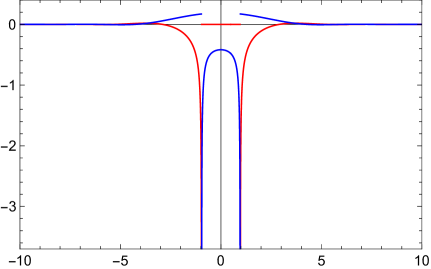
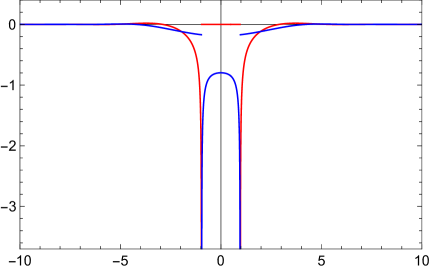
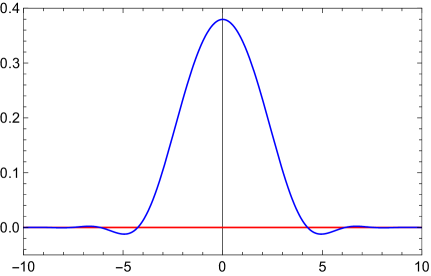
Figure 2: The state integral $\chi_{\bm{4}_{1}}(u;\hbar)$ in the closed form of Eq. (5.187) as a function of $x\in{\mathbb{R}}$, at the bottom, and its components $\chi_{\bm{4}_{1}}^{(\pm)}(u;\hbar)$ in Eq. (5.188), in the top left and top right, respectively, for $P=Q=1$. The real and imaginary parts are displayed in blue and red.

We will now comment on the most notable features of the exact expression for the non-perturbative wave function in Eq. (5.187). It will be useful to introduce

$$\chi_{\bm{4}_{1}}^{(\pm)}(u;\hbar)=\frac{{\rm e}^{\frac{x^{2}Q}{2\pi{\rm i}P}+x\left(2Q-\frac{1}{2}-\frac{Q}{2P}\right)}}{{\rm i}{\mathsf{b}}Q\sqrt{\Delta({\rm e}^{xQ})}}\sum_{k=0}^{PQ-1}{\rm e}^{-\frac{2xk}{P}}{\rm e}^{F_{k}(y_{\pm}(x))}\,,$$ (5.188)

where again $x\in{\mathbb{R}}$, so that we write

$$\chi_{\bm{4}_{1}}(u;\hbar)=\chi_{\bm{4}_{1}}^{(+)}(u;\hbar)-\chi_{\bm{4}_{1}}^{(-)}(u;\hbar)\,.$$ (5.189)

Observe that the $S$-duality, which acts in the rational case via $P\leftrightarrow Q$ and $x\rightarrow xQ/P$, leaves $\Delta({\rm e}^{xQ})$ unchanged while transforming $y_{\pm,k}(x)$ into $y_{\pm,k}(x)Q/P$, and therefore the closed formula for the state integral of the $\bm{4}_{1}$-knot in Eq. (5.187) is $S$-invariant, as expected. Similarly, we also find that its components in Eq. (5.188) are themselves invariant under $S$-duality. Moreover, we have that

$$\Im(\chi_{\bm{4}_{1}}^{(+)}(u;\hbar))=\Im(\chi_{\bm{4}_{1}}^{(-)}(u;\hbar))\,,$$ (5.190)

while both $\Re(\chi_{\bm{4}_{1}}^{(\pm)}(u;\hbar))$ and $\Im(\chi_{\bm{4}_{1}}^{(\pm)}(u;\hbar))$ are even functions of $x\in{\mathbb{R}}$ with singularities located at the points

$$x=\frac{1}{Q}\log\left(\frac{3\pm\sqrt{5}}{2}\right)\,,$$ (5.191)

which correspond to the zeros of $\Delta({\rm e}^{xQ})$ in Eq. (5.182) and, as such, do not depend on the value of $P$. The discontinuities of $\Re(\chi_{\bm{4}_{1}}^{(\pm)}(u;\hbar))$ cancel with each other to give a smooth difference function in Eq. (5.189), which is itself symmetric under $x\rightarrow-x$. Remarkably, we find that the total state integral $\chi_{\bm{4}_{1}}(u;\hbar)$ is a real-valued smooth square-integrable function of $x\in{\mathbb{R}}$, while both functions $\chi_{\bm{4}_{1}}^{(\pm)}(u;\hbar)$ are neither real-valued, smooth, or square-integrable when considered separately. To illustrate these properties with an example, we show in Fig. 2 the functions in Eqs. (5.187), (5.188) for the benchmark choice $P=Q=1$. The same features and similar functional profiles are verified for various choices of $P,Q\in{\mathbb{Z}}_{>0}$ coprime. We show in Fig. 3 the full non-perturbative wave function for a sample of small values of ${\mathsf{b}}^{2}\in{\mathbb{Q}}_{>0}$.

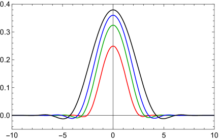
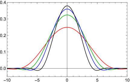
Figure 3: The real part of the state integral $\chi_{\bm{4}_{1}}(u;\hbar)$ in the closed form of Eq. (5.187) as a function of $x\in{\mathbb{R}}$ for rational values of ${\mathsf{b}}^{2}$. We show ${\mathsf{b}}^{2}=1/3$ (in red), $1/2$ (in green), $2/3$ (in blue), and $1$ (in black), on the left, and ${\mathsf{b}}^{2}=3$ (in red), $2$ (in green), $3/2$ (in blue), and $1$ (in black), on the right. The imaginary part is identically zero and not displayed explicitly in the plot.

We observe that $\chi_{\bm{4}_{1}}(u;\hbar)$ has a Gaussian-type profile centered at $x=0$ with lateral oscillations around the $x$-axis, which are quickly dampened. The peak at the origin can be evaluated directly from Eqs. (5.181), (5.186), and (5.187) for arbitrary $P,Q\in{\mathbb{Z}}_{>0}$ coprime, yielding a result which is left unchanged by $P\leftrightarrow Q$, as expected from the $S$-invariance of the state integral and evident in Fig. 3. In particular, the highest peak corresponds to the choice $P=Q=1$ and amounts to

$$\chi_{\bm{4}_{1}}(0;2\pi)=\frac{2}{\sqrt{3}}\sinh\left(\frac{V}{2\pi}\right)\,,\quad V=2\,\Im\left(\text{Li}_{2}\left({\rm e}^{\frac{\pi{\rm i}}{3}}\right)\right)=2.0298832\dots\,,$$ (5.192)

where $\text{Li}_{2}(z)$ is the standard dilogarithm and $V$ is the volume of the $\bm{4}_{1}$-knot, as expected garou-kas . As ${\mathsf{b}}^{2}>1$ increases, the shape of the function $\chi_{\bm{4}_{1}}(u;\hbar)$ widens, while for decreasing ${\mathsf{b}}^{2}<1$, the shape tightens, and in both cases the peak lowers.

We point out that the structure of the exact wave function at rational values for the figure-eight knot obtained here is tantalizingly close to what has been found in the spectral theory of quantum mirror curves. The case of $\hbar=2\pi$, corresponding to ${\mathsf{b}}^{2}=1$, was studied in detail in mz-wv ; mz-wv2 . As in Eq. (5.189), the wave functions in mz-wv ; mz-wv2 are the sums of two individual functions corresponding to two different choices of branch cut in the mirror curve. Each component function is singular when considered alone. Still, the singularities cancel each other in the sum, and one obtains a square-integrable wave function in the end, similar to the one plotted in Fig. 2. We observe that, in the case of the quantum mirror curves studied in mz-wv ; mz-wv2 , one is working with exponentiated Heisenberg operators, and the resulting wave functions do not satisfy the nodal theorem for the Schrödinger operator typical of confining potentials, since the ground state changes sign in a small region. This same feature is also evident in our plots for the exact wave functions of the $\bm{4}_{1}$-knot at rational points shown in Fig. 2 and Fig. 3. Such a property suggests that the wave function occurring in complex CS theory is a ground state for an appropriate spectral definition of the quantum $A$-polynomial. We will return to this point in the conclusions.

Finally, let us stress that the results above provide a third method for the computation of the exact wave function at rational values of $\hbar$ to be compared with the previous two presented in Section 3. We conclude by verifying numerically that our closed formula in Eq. (5.187) for the state integral of the figure-eight knot at rational values matches the results of Section 4.1. Specifically, the two components $\chi_{\bm{4}_{1}}^{(\pm)}(u;\hbar)$ in Eq. (5.188) can be identified with the two terms in the holomorphic/antiholomorphic block decomposition in Eq. (4.134), which correspond to the conjugate and geometric classical branches, respectively. This identification will be formally clarified in the discussion in the following section.

5.2 Factorization and two special subcases

Let us apply the explicit formula for the Faddeev’s quantum dilogarithm at the rational point ${\mathsf{b}}^{2}=P/Q$, $P,Q\in{\mathbb{Z}}_{>0}$ coprime, in Eq. (C.11) to the expression for $F_{k}(y(x))$, $0\leq k\leq PQ-1$, which is given in Eq. (5.186). After appropriately rearranging the terms, we find the factorization

$${\rm e}^{F_{k}(y(x))}={\rm e}^{F_{0}(y(x))}f_{0,k}(y(x))f_{1,k}(y(x))f_{2,k}(y(x))\,,$$ (5.193)

where we have introduced the functions

$$f_{0,k}(y(x)) =\left[\left(1-{\rm e}^{Q(x-y(x))+\pi{\rm i}(P+Q)}\right)\left(1-{\rm e}^{Qy(x)+\pi{\rm i}(P+Q)}\right)\right]^{\frac{k}{PQ}}\,,$$ (5.194a)

$$f_{1,k}(y(x)) =\prod_{j=1}^{Q-1}\left[\frac{\left(1+{\rm e}^{x-y(x)+\frac{\pi{\rm i}P}{Q}(2j+1)}\right)\left(1+{\rm e}^{y(x)+\frac{\pi{\rm i}P}{Q}(2j+1+2k/P)}\right)}{\left(1+{\rm e}^{x-y(x)+\frac{\pi{\rm i}P}{Q}(2j+1-2k/P)}\right)\left(1+{\rm e}^{y(x)+\frac{\pi{\rm i}P}{Q}(2j+1)}\right)}\right]^{j\over Q}\,,$$ (5.194b)

$$f_{2,k}(y(x)) =\prod_{j=1}^{P-1}\left[\frac{\left(1+{\rm e}^{\frac{Q}{P}(x-y(x))+\frac{\pi{\rm i}Q}{P}(2j+1)}\right)\left(1+{\rm e}^{\frac{Q}{P}y(x)+\frac{\pi{\rm i}Q}{P}(2j+1+2k/Q)}\right)}{\left(1+{\rm e}^{\frac{Q}{P}(x-y(x))+\frac{\pi{\rm i}Q}{P}(2j+1-2k/Q)}\right)\left(1+{\rm e}^{\frac{Q}{P}y(x)+\frac{\pi{\rm i}Q}{P}(2j+1)}\right)}\right]^{j\over P}\,,$$ (5.194c)

for $0\leq k\leq PQ-1$. Thus, we can write the state integral for arbitrary rational values of ${\mathsf{b}}^{2}$ in Eq. (5.187) in the equivalent form

$$\chi_{\bm{4}_{1}}(u;\hbar)=\frac{{\rm e}^{\frac{x^{2}Q}{2\pi{\rm i}P}+x\left(2Q-\frac{1}{2}-\frac{Q}{2P}\right)}}{{\rm i}{\mathsf{b}}Q\sqrt{\Delta({\rm e}^{xQ})}}\left[{\rm e}^{F_{0}(y_{+}(x))}{\cal A}(y_{+}(x))-{\rm e}^{F_{0}(y_{-}(x))}{\cal A}(y_{-}(x))\right]\,,$$ (5.195)

where the function ${\cal A}(y(x))$ is defined by

$${\cal A}(y(x))=\sum_{k=0}^{PQ-1}{\rm e}^{-\frac{2xk}{P}}f_{0,k}(y(x))f_{1,k}(y(x))f_{2,k}(y(x))\,,$$ (5.196)

and $F_{0}(y(x))$ can be expressed explicitly in terms of more elementary functions using Eq. (C.11). We stress that the formula for the state integral in Eq. (5.195) allows us to more clearly separate the contributions from the two non-abelian saddle connections of the $\bm{4}_{1}$-knot labeled by $\alpha=\text{geom},\text{conj}$, as in the holomorphic/antiholomorphic block decomposition in Eq. (3.51). Indeed, expanding the functions $F_{0}(y_{\mp}(x))$ in powers of $X,X^{-1}$ and suitably identifying the terms in the expansions, we derive the integer constants $c_{\pm s}$, $s\in{\mathbb{Z}}_{>0}$, previously written in Eqs. (4.144a), (4.144b), for the geometric and conjugate branches, respectively.

Let us consider now the two special choices ${\mathsf{b}}^{2}=P$ and ${\mathsf{b}}^{2}=1/Q$ for $P,Q\in{\mathbb{Z}}_{>0}$. In both subcases, the closed formula for the state integral of the figure-eight knot in Eq. (5.195) specializes in a correspondingly simpler and more compact form. We start by choosing ${\mathsf{b}}^{2}=P$ positive integer. After some manipulations, the factorization formula in Eq. (5.193) reduces to the relation

$${\rm e}^{F_{k}(y(x))}={\rm e}^{F_{0}(y(x))}\prod_{j=0}^{k-1}\left(1+{\rm e}^{\frac{1}{P}(x-y(x))-\frac{\pi{\rm i}}{P}(2j+1)}\right)\left(1+{\rm e}^{\frac{1}{P}y(x)+\frac{\pi{\rm i}}{P}(2j+1)}\right)\,,$$ (5.197)

where $0\leq k\leq P-1$, and we can write the state integral in Eq. (5.195) for ${\mathsf{b}}^{2}=P$ as

$$\chi_{\bm{4}_{1}}(u;\hbar)=\frac{{\rm e}^{\frac{x^{2}}{2\pi{\rm i}P}+x\left(\frac{3}{2}-\frac{1}{2P}\right)}}{{\rm i}{\mathsf{b}}\sqrt{\Delta({\rm e}^{x})}}\left[{\rm e}^{F_{0}(y_{+}(x))}{\cal B}(y_{+}(x))-{\rm e}^{F_{0}(y_{-}(x))}{\cal B}(y_{-}(x))\right]\,,$$ (5.198)

where the function ${\cal B}(y(x))$ is simply defined by

$${\cal B}(y(x))=\sum_{k=0}^{P-1}{\rm e}^{-\frac{2xk}{P}}\prod_{j=0}^{k-1}\left(1+{\rm e}^{\frac{1}{P}(x-y(x))-\frac{\pi{\rm i}}{P}(2j+1)}\right)\left(1+{\rm e}^{\frac{1}{P}y(x)+\frac{\pi{\rm i}}{P}(2j+1)}\right)\,,$$ (5.199)

and $F_{0}(y(x))$ can be expressed explicitly by means of Eq. (C.13a). Let us now choose ${\mathsf{b}}^{-2}=Q$ positive integer. After some manipulations, the factorization formula in Eq. (5.193) becomes

$${\rm e}^{F_{k}(y(x))}={\rm e}^{F_{0}(y(x))}\prod_{j=0}^{k-1}\left(1+{\rm e}^{x-y(x)-\frac{\pi{\rm i}}{Q}(2j+1)}\right)\left(1+{\rm e}^{y(x)+\frac{\pi{\rm i}}{Q}(2j+1)}\right)\,,$$ (5.200)

and the exact partition function in Eq. (5.195) for ${\mathsf{b}}^{2}=1/Q$ assumes the simplified form

$$\chi_{\bm{4}_{1}}(u;\hbar)=\frac{{\rm e}^{\frac{x^{2}Q}{2\pi{\rm i}}+x\left(\frac{3Q}{2}-\frac{1}{2}\right)}}{{\rm i}{\mathsf{b}}Q\sqrt{\Delta({\rm e}^{xQ})}}\left[{\rm e}^{F_{0}(y_{+}(x))}{\cal C}(y_{+}(x))-{\rm e}^{F_{0}(y_{-}(x))}{\cal C}(y_{-}(x))\right]\,,$$ (5.201)

where the function ${\cal C}(y(x))$ is given by

$${\cal C}(y(x))=\sum_{k=0}^{Q-1}{\rm e}^{-2xk}\prod_{j=0}^{k-1}\left(1+{\rm e}^{x-y(x)-\frac{\pi{\rm i}}{Q}(2j+1)}\right)\left(1+{\rm e}^{y(x)+\frac{\pi{\rm i}}{Q}(2j+1)}\right)\,,$$ (5.202)

and $F_{0}(y(x))$ can be expressed explicitly by means of Eq. (C.13b). We observe that the reduced factorization formulae in Eq. (5.197), (5.200) for ${\mathsf{b}}^{2}=P$ and ${\mathsf{b}}^{2}=1/Q$ with $P,Q\in{\mathbb{Z}}_{>0}$ can alternatively be derived by substituting ${\rm i}{\mathsf{b}}k/P={\rm i}{\mathsf{b}}^{-1}k$ and ${\rm i}{\mathsf{b}}k/P={\rm i}{\mathsf{b}}k$ into the arguments of the Faddeev’s quantum dilogarithms in Eq. (5.186) and applying the periodicity properties in Eqs. (C.8c), (C.8d) and Eqs. (C.8a), (C.8b) to the resulting formulae for $F_{k}(y(x))$, $0\leq k\leq PQ-1$, respectively. In the general case of ${\mathsf{b}}^{2}=P/Q$, instead, we cannot resort to these quasi-periodicity properties because the functions $F_{k}(y(x))$ contain, in general, a fractional shift in the arguments of the Faddeev’s quantum dilogarithms.

6 Conclusions

In this paper, we have made various observations on the structure of the wave functions in CS theory with gauge group $\text{SL}(2,{\mathbb{C}})$ on the complement of a hyperbolic knot in the three-sphere. We have first conjectured explicit integrality properties for the resummed WKB expansion of the wave function, which can be tested directly using the decomposition into holomorphic/anti-holomorphic blocks. Our integrality conjecture guarantees that the singularities appearing in the holomorphic blocks at rational values of $\hbar$ get canceled against those occurring in the corresponding anti-holomorphic blocks. We have then developed various techniques to compute the wave function in the rational case effectively. In particular, we have analyzed the quantum $A$-polynomial at rational points by exploiting the underlying quasi-periodic structure, and we have solved the associated $q$-dfference equation in closed form in the general cases of order two and three. The calculation methods we have introduced have been applied to the examples of the figure-eight and the three-twist knots, and our conjectural statements have been verified. Finally, we have performed a direct evaluation of the Andersen–Kashaev state integral of the figure-eight knot at rational values, which gave us further insights into the properties of the exact wave functions. All computational approaches have yielded compatible results.

Our investigation raises two main questions. The first one concerns the interpretation of the integrality structure of the resummed WKB expansion of the wave function in terms of an enumerative problem, or a BPS counting problem, in the dual supersymmetric theory dgg . The second one concerns the shape of the wave function obtained by directly evaluating the state integral. As highlighted in Section 5, this is enticingly similar to the functional profiles of the ground state wave functions computed in the context of the TS/ST correspondence mz-wv ; mz-wv2 . This observation raises the issue of understanding the AJ conjecture from a purely quantum mechanical point of view. The AJ conjecture can be explained, a priori, as a consequence of the quantization of the classical moduli space described by the $A$-polynomial, as pointed out in gukov and briefly recalled in Section 2. However, the precise details of this quantization procedure still need to be fully understood from a physical perspective. We know that the quantization is non-trivial and cannot be obtained by simply promoting the classical variables $X,P$ to Weyl operators. In addition, the classical phase space is not compact, which carries various problems concerning its appropriate quantization. From a quantum mechanical angle, in such a situation, we would generically expect to have at most metastable states with complex energies. We are, therefore, tempted to conjecture that the observed non-trivial quantization of the $A$-polynomial is required to obtain a normalizable wave function with precisely zero energy. We hope to address this question in the near future.

Appendix A Computing the $\epsilon$-expansions

For completeness, we include here the details of the computations performed in Section 3.2. We observe that, as a consequence of Eqs. (3.41), (3.45), the coefficient functions $\hat{a}_{\pm n}(q)$ satisfy the relation

$$\hat{a}_{\pm n}(q)q^{-\sigma_{\pm n}}=\sum_{k|n}kD_{\pm k}\left(q^{n\over k}\right)q^{-{n\over k}\sigma_{\pm k}}\sum_{j=0}^{k-1}q^{{n\over k}j}\,,\quad n\in{\mathbb{Z}}_{>0}\,,$$ (A.1)

and we write the ${\mathbb{Z}}$-polynomials $D_{\pm k}(q)$ explicitly as

$$D_{\pm k}(q)=\sum_{\ell=0}^{\deg{D_{\pm k}}}D_{\pm k,\ell}\;q^{\ell}\,,\quad k\in{\mathbb{Z}}_{>0}\,,$$ (A.2)

where $D_{\pm k,\ell}$ is an integer and $\deg{D_{\pm k}}$ denotes the degree of the polynomial. Let us now take

$$q={\rm e}^{2\pi{\rm i}{P\over Q}}\,,\quad P,Q\in{\mathbb{Z}}_{>0}\;\;\text{coprime}\,,$$ (A.3)

while we introduce

$$q_{\epsilon}={\rm e}^{{\rm i}\hbar_{\epsilon}}\,,\quad\hbar_{\epsilon}=2\pi{P\over Q}+\epsilon\,,\quad 0<\epsilon\ll 1\,,$$ (A.4)

and consider the limit $\epsilon\rightarrow 0$. In the case $n=sQ$, $s\in{\mathbb{Z}}_{>0}$, we have the $\epsilon$-expansions

$$D_{\pm k}\left(q_{\epsilon}^{sQ\over k}\right) =\left(1+{\rm i}\epsilon\,q{\partial\over\partial q}\right)D_{\pm k}\left(q^{sQ\over k}\right)+{\cal O}(\epsilon^{2})\,,$$ (A.5a)

$$\sum_{j=0}^{k-1}q_{\epsilon}^{{sQ\over k}(j-\sigma_{\pm k})} =\left(1+{\rm i}\epsilon\,q{\partial\over\partial q}\right)\sum_{j=0}^{k-1}q^{{sQ\over k}(j-\sigma_{\pm k})}+{\cal O}(\epsilon^{2})\,,$$ (A.5b)

and therefore also

$$\hat{a}_{\pm sQ}(q_{\epsilon})q_{\epsilon}^{-\sigma_{\pm sQ}}=\left(1+{\rm i}\epsilon\,q{\partial\over\partial q}\right)\hat{a}_{\pm sQ}(q)q^{-\sigma_{\pm sQ}}+{\cal O}(\epsilon^{2})\,.$$ (A.6)

We now observe that

$$\frac{1}{q_{\epsilon}^{sQ}-1}=-\frac{{\rm i}}{sQ\epsilon}-\frac{1}{2}+{\cal O}(\epsilon)\,,$$ (A.7)

and, combining Eqs. (A.6), (A.7), we finally obtain the NLO $\epsilon$-expansion in Eq. (3.60a). On the dual side, we consider

$$q_{D}=q^{Q^{2}\over P^{2}}={\rm e}^{2\pi{\rm i}{Q\over P}}\,,\quad q_{\epsilon,D}={\rm e}^{4\pi^{2}{\rm i}\over\hbar_{\epsilon}}\,,$$ (A.8)

and take again the limit $\epsilon\rightarrow 0$. It follows that

$$q_{\epsilon,D}=q_{D}\,{\rm e}^{-\epsilon{Q^{2}\over P^{2}}+{\cal O}(\epsilon^{2})}\,.$$ (A.9)

Similarly to the case above, when $n=sP$, $s\in{\mathbb{Z}}_{>0}$, we have the $\epsilon$-expansions

$$D_{\pm k}\left(q_{\epsilon,D}^{sP\over k}\right) =\left(1-{\rm i}\epsilon\frac{Q^{2}}{P^{2}}\,q_{D}{\partial\over\partial q_{D}}\right)D_{\pm k}\left(q_{D}^{sP\over k}\right)+{\cal O}(\epsilon^{2})\,,$$ (A.10a)

$$\sum_{j=0}^{k-1}q_{\epsilon,D}^{{sP\over k}(j-\sigma_{\pm k})} =\left(1-{\rm i}\epsilon\frac{Q^{2}}{P^{2}}\,q_{D}{\partial\over\partial q_{D}}\right)\sum_{j=0}^{k-1}q_{D}^{{sP\over k}(j-\sigma_{\pm k})}+{\cal O}(\epsilon^{2})\,,$$ (A.10b)

and therefore also

$$\hat{a}_{\pm sP}(q_{\epsilon,D})q_{\epsilon,D}^{-\sigma_{\pm sP}}=\left(1-{\rm i}\epsilon\frac{Q^{2}}{P^{2}}\,q_{D}{\partial\over\partial q_{D}}\right)\hat{a}_{\pm sP}(q_{D})q_{D}^{-\sigma_{\pm sP}}+{\cal O}(\epsilon^{2})\,.$$ (A.11)

Finally, we note that

$$\frac{1}{q_{\epsilon,D}^{sP}-1}=\frac{{\rm i}P}{sQ^{2}\epsilon}-\frac{1}{2}+\frac{{\rm i}}{2\pi sQ}+{\cal O}(\epsilon)\,,$$ (A.12)

and, combining Eqs. (A.11), (A.12), we obtain the NLO $\epsilon$-expansion in Eq. (3.60b).

Appendix B An alternative way of obtaining the integer sequences

We present an alternative, simple way of computing the integer sequences $\{c_{\pm s}\}$, $s\in{\mathbb{Z}}_{>0}$, defined in Eqs. (3.65), (3.66), using the results on the exact wave function at rational values obtained in Section 3.3. Let us denote by $\phi_{(\pm)}^{\rm WKB}(X;q)$ the contributions to the holomorphic block $\phi^{\rm WKB}(X;q)$ from the positive and negative powers of $X$, respectively, so that Eq. (3.40) assumes the form

$$\phi^{\rm WKB}(X;q)=\phi_{(+)}^{\rm WKB}(X;q)+\phi_{(-)}^{\rm WKB}(X;q)\,,$$ (B.1)

and analogously for the antiholomorphic block $\phi^{\rm WKB}(X_{D};q_{D})$. We fix $\hbar$ as in Eq. (3.53) and consider the formula for $\phi^{\rm WKB}(X;q)+\phi^{\rm WKB}(X_{D};q_{D})$ in Eq. (3.82). Setting the values $P=Q=1$, the $X$-series component becomes

$$\frac{{\rm i}}{2\pi}\sum_{s\geq 1}\frac{X^{s}}{s^{2}}\left[\left(2\pi{\rm i}s+1-s\log X+4\pi{\rm i}\sigma_{s}\right)\hat{a}_{s}(1)-4\pi{\rm i}\frac{\partial}{\partial q}\hat{a}_{s}(q)_{q=1}\right]\,.$$ (B.2)

Let us now go back to the sum in Eq. (3.54) and apply the change of variable $\hbar\rightarrow-\hbar$, which transforms $q,q_{D}$ into $q^{-1},q_{D}^{-1}$, while we keep $X,X_{D}$ fixed. After performing the $\epsilon$-expansion as in Section 3.2 and then taking $P=Q=1$ in the sum $\phi_{(+)}^{\rm WKB}(X;q^{-1})+\phi_{(+)}^{\rm WKB}(X_{D};q_{D}^{-1})$, we find the very close but not identical quantity

$$\frac{{\rm i}}{2\pi}\sum_{s\geq 1}\frac{X^{s}}{s^{2}}\left[\left(2\pi{\rm i}s-1+s\log X+4\pi{\rm i}\sigma_{s}\right)\hat{a}_{s}(1)-4\pi{\rm i}\frac{\partial}{\partial q}\hat{a}_{s}(q)_{q=1}\right]\,.$$ (B.3)

By taking the difference of Eqs. (B.2), (B.3), we arrive at

$$\frac{{\rm i}}{\pi}\sum_{s\geq 1}\frac{X^{s}}{s^{2}}(1-s\log X)\hat{a}_{s}(1)\,.$$ (B.4)

Therefore, if we compute the function

$$\left[\left(\phi_{(+)}^{\rm WKB}(X;q)+\phi_{(+)}^{\rm WKB}(X_{D};q_{D})\right)-\left(\phi_{(+)}^{\rm WKB}(X;q^{-1})+\phi_{(+)}^{\rm WKB}(X_{D};q_{D}^{-1})\right)\right]_{P=Q=1}\,,$$ (B.5)

its expansion in powers of $X$ is precisely the series in Eq. (B.4). From the coefficients of this expansion, we can easily extract the desired integers $c_{s}=\hat{a}_{s}(1)$ for $s\in{\mathbb{Z}}_{>0}$. Let us now consider the $X^{-1}$-series component of Eq. (3.82). Again, setting the values $P=Q=1$, we find

$$\frac{{\rm i}}{2\pi}\sum_{s\geq 1}\frac{X^{-s}}{s^{2}}\left[\left(2\pi{\rm i}s+1+s\log X\right)\hat{a}_{-s}(1)-4\pi{\rm i}\frac{\partial}{\partial q}\hat{a}_{-s}(q)_{q=1}\right]\,.$$ (B.6)

As before, we go back to the sum in Eq. (3.54) and apply the change of variable $\hbar\rightarrow-\hbar$, which transforms $q,q_{D}$ into $q^{-1},q_{D}^{-1}$, while we keep $X,X_{D}$ fixed. After performing the $\epsilon$-expansion as in Section 3.2 and then taking $P=Q=1$ in the sum $\phi_{(-)}^{\rm WKB}(X;q^{-1})+\phi_{(-)}^{\rm WKB}(X_{D};q_{D}^{-1})$, we find the slightly different quantity

$$\frac{{\rm i}}{2\pi}\sum_{s\geq 1}\frac{X^{-s}}{s^{2}}\left[\left(2\pi{\rm i}s-1-s\log X\right)\hat{a}_{-s}(1)-4\pi{\rm i}\frac{\partial}{\partial q}\hat{a}_{-s}(q)_{q=1}\right]\,.$$ (B.7)

By taking the difference of Eqs. (B.6), (B.7), we arrive at

$$\frac{{\rm i}}{\pi}\sum_{s\geq 1}\frac{X^{-s}}{s^{2}}(1+s\log X)\hat{a}_{-s}(1)\,.$$ (B.8)

Accordingly, if we compute the function

$$\left[\left(\phi_{(-)}^{\rm WKB}(X;q)+\phi_{(-)}^{\rm WKB}(X_{D};q_{D})\right)-\left(\phi_{(-)}^{\rm WKB}(X;q^{-1})+\phi_{(-)}^{\rm WKB}(X_{D};q_{D}^{-1})\right)\right]_{P=Q=1}\,,$$ (B.9)

its expansion in powers of $X^{-1}$ is precisely the series in Eq. (B.8). From the coefficients of this expansion, we can straightforwardly obtain the desired integers $c_{-s}=\hat{a}_{-s}(1)$ for $s\in{\mathbb{Z}}_{>0}$.

Appendix C Faddeev’s quantum dilogarithm and other special functions

The quantum dilogarithm is the function of two variables defined by the series fk ; Kirillov

$$(zq^{\alpha};\,q)_{\infty}=\prod_{n=0}^{\infty}(1-zq^{\alpha+n})\,,\quad\alpha\in{\mathbb{R}}\,,$$ (C.1)

which is analytic in $z,q\in{\mathbb{C}}$ with $|z|,|q|<1$, and it has asymptotic expansions around $q$ a root of unity. Furthermore, we denote by

$$(z;\,q)_{m}=\prod_{n=0}^{m-1}(1-zq^{n})=\frac{(z;\,q)_{\infty}}{(zq^{m};\,q)_{\infty}}\,,\quad m\in{\mathbb{Z}}\,,$$ (C.2)

with $(z;\,q)_{0}=1$, the $q$-shifted factorials, also known as $q$-Pochhammer symbols. Faddeev’s quantum dilogarithm $\Phi_{{\mathsf{b}}}(z)$ is defined in the strip $|\Im(z)|<|\Im(c_{{\mathsf{b}}})|$ as faddeev ; fk

$$\Phi_{{\mathsf{b}}}(z)=\exp\left(\int_{{\mathbb{R}}+{\rm i}\epsilon}\frac{{\rm e}^{-2{\rm i}zy}}{4\sinh(y{\mathsf{b}})\sinh(y{\mathsf{b}}^{-1})}\frac{{\rm d}y}{y}\right)\,,$$ (C.3)

which can be analytically continued to the whole complex $z$-plane for all values of ${\mathsf{b}}$ such that ${\mathsf{b}}^{2}\notin{\mathbb{R}}_{\leq 0}$. When $\Im({\mathsf{b}}^{2})>0$, the formula in Eq. (C.3) is equivalent to

$$\Phi_{{\mathsf{b}}}(z)=\frac{({\rm e}^{2\pi{\mathsf{b}}(z+c_{{\mathsf{b}}})};\,q)_{\infty}}{({\rm e}^{2\pi{\mathsf{b}}^{-1}(z-c_{{\mathsf{b}}})};\,\tilde{q})_{\infty}}=\prod_{n=0}^{\infty}\frac{1-{\rm e}^{2\pi{\mathsf{b}}(z+c_{{\mathsf{b}}})}q^{n}}{1-{\rm e}^{2\pi{\mathsf{b}}^{-1}(z-c_{{\mathsf{b}}})}\tilde{q}^{n}}\,,$$ (C.4)

where $q={\rm e}^{2\pi\text{i}{\mathsf{b}}^{2}}$, $\tilde{q}={\rm e}^{-2\pi\text{i}{\mathsf{b}}^{-2}}$, and $c_{{\mathsf{b}}}={\rm i}({\mathsf{b}}+{\mathsf{b}}^{-1})/2$. It follows that $\Phi_{{\mathsf{b}}}(z)$ is a meromorphic function with poles at the points $z=c_{{\mathsf{b}}}+{\rm i}m{\mathsf{b}}+{\rm i}n{\mathsf{b}}^{-1}$ and zeros at the points $z=-c_{{\mathsf{b}}}-{\rm i}m{\mathsf{b}}-{\rm i}n{\mathsf{b}}^{-1}$ for $m,n\in{\mathbb{N}}$. It satisfies the inversion property

$$\Phi_{{\mathsf{b}}}(z)\Phi_{{\mathsf{b}}}(-z)={\rm e}^{\pi{\rm i}z^{2}}\Phi_{{\mathsf{b}}}(0)^{2}\,,\quad\Phi_{{\mathsf{b}}}(0)=\left(\frac{q}{\tilde{q}}\right)^{1/48}={\rm e}^{\pi{\rm i}({\mathsf{b}}^{2}+{\mathsf{b}}^{-2})/24}\,,$$ (C.5)

the complex conjugation property

$$\Phi_{{\mathsf{b}}}(z)^{*}=\Phi_{{\mathsf{b}}^{*}}(z^{*})^{-1}\,,$$ (C.6)

and the symmetries

$$\Phi_{{\mathsf{b}}}(z)=\Phi_{-{\mathsf{b}}}(z)=\Phi_{\frac{1}{{\mathsf{b}}}}(z)\,.$$ (C.7)

Moreover, Faddeev’s quantum dilogarithm is a quasi-periodic function. Precisely, as a direct consequence of its definition in Eq. (C.4), we find the relations

$$\Phi_{{\mathsf{b}}}(z+{\rm i}{\mathsf{b}}k) =\Phi_{{\mathsf{b}}}(z)\prod_{j=0}^{k-1}\left(1+{\rm e}^{2\pi{\mathsf{b}}z+\pi{\rm i}{\mathsf{b}}^{2}(2j+1)}\right)^{-1}\,,$$ (C.8a)

$$\Phi_{{\mathsf{b}}}(z-{\rm i}{\mathsf{b}}k) =\Phi_{{\mathsf{b}}}(z)\prod_{j=0}^{k-1}\left(1+{\rm e}^{2\pi{\mathsf{b}}z-\pi{\rm i}{\mathsf{b}}^{2}(2j+1)}\right)\,,$$ (C.8b)

$$\Phi_{{\mathsf{b}}}(z+{\rm i}{\mathsf{b}}^{-1}k) =\Phi_{{\mathsf{b}}}(z)\prod_{j=0}^{k-1}\left(1+{\rm e}^{2\pi{\mathsf{b}}^{-1}z+\pi{\rm i}{\mathsf{b}}^{-2}(2j+1)}\right)^{-1}\,,$$ (C.8c)

$$\Phi_{{\mathsf{b}}}(z-{\rm i}{\mathsf{b}}^{-1}k) =\Phi_{{\mathsf{b}}}(z)\prod_{j=0}^{k-1}\left(1+{\rm e}^{2\pi{\mathsf{b}}^{-1}z-\pi{\rm i}{\mathsf{b}}^{-2}(2j+1)}\right)\,,$$ (C.8d)

where $k\in{\mathbb{Z}}_{>0}$. If we consider the special case of ${\mathsf{b}}^{2}\in{\mathbb{Q}}_{>0}$ and, specifically, take

$${\mathsf{b}}^{2}=\frac{P}{Q}\,,\quad P,Q\in{\mathbb{Z}}_{>0}\;\;\text{coprime}\,,$$ (C.9)

then the periodicity formulae above give in particular

$$\Phi_{{\mathsf{b}}}(z+{\rm i}{\mathsf{b}}Q) =\Phi_{{\mathsf{b}}}(z)\left(1+{\rm e}^{2\pi{\mathsf{b}}Qz+\pi{\rm i}PQ}\right)^{-1}\,,$$ (C.10a)

$$\Phi_{{\mathsf{b}}}(z-{\rm i}{\mathsf{b}}Q) =\Phi_{{\mathsf{b}}}(z)\left(1+{\rm e}^{2\pi{\mathsf{b}}Qz-\pi{\rm i}PQ}\right)^{\,}.$$ (C.10b)

Finally, in the above rational case of Eq. (C.9), it was shown in garou-kas that Faddeev’s quantum dilogarithm can be expressed as

$$\Phi_{{\mathsf{b}}}\left(\frac{z}{2\pi{\mathsf{b}}}\right)=\exp\left[\frac{{\rm i}}{2\pi PQ}\right. \text{Li}_{2}\left({\rm e}^{w(z)}\right)+\left(1+\frac{{\rm i}w(z)}{2\pi PQ}\right)\log\left(1-{\rm e}^{w(z)}\right)$$ (C.11)

$$\left.-\log D_{Q}\left({\rm e}^{\frac{w(z)}{Q}};\,{\rm e}^{2\pi{\rm i}\frac{P}{Q}}\right)-\log D_{P}\left({\rm e}^{\frac{w(z)}{P}};\,{\rm e}^{2\pi{\rm i}\frac{Q}{P}}\right)\right]\,,$$

where $w(z)=Qz+\pi{\rm i}(P+Q)$, $\text{Li}_{2}(z)$ is the standard dilogarithm, and

$$D_{N}(z;\,q)=\prod_{j=1}^{N-1}\left(1-zq^{j}\right)^{j/N}\,,\quad N\in{\mathbb{Z}}_{>0}\,,$$ (C.12)

is the $N$-th cyclic quantum dilogarithm with $D_{1}(z;q)=1$. In the special subcases of ${\mathsf{b}}^{2}=P$ positive integer and ${\mathsf{b}}^{2}=1/Q$ positive unit fraction, the formula in Eq. (C.11) simplifies into

$$\Phi_{{\mathsf{b}}}\left(\frac{z}{2\pi{\mathsf{b}}}\right)= \exp\left[\frac{{\rm i}}{2\pi P}\text{Li}_{2}\left(-{\rm e}^{z+\pi{\rm i}P}\right)+\left(\frac{P-1}{2P}+\frac{{\rm i}z}{2\pi P}\right)\log\left(1+{\rm e}^{z+\pi{\rm i}P}\right)\right.$$ (C.13a)

$$\left.\quad\quad\;-\log D_{P}\left(-{\rm e}^{\frac{z}{P}+\frac{\pi{\rm i}}{P}};\,{\rm e}^{\frac{2\pi{\rm i}}{P}}\right)\right]\,,$$

$$\Phi_{{\mathsf{b}}}\left(\frac{z}{2\pi{\mathsf{b}}}\right)= \exp\left[\frac{{\rm i}}{2\pi Q}\text{Li}_{2}\left(-{\rm e}^{Qz+\pi{\rm i}Q}\right)+\left(\frac{Q-1}{2Q}+\frac{{\rm i}z}{2\pi}\right)\log\left(1+{\rm e}^{Qz+\pi{\rm i}Q}\right)\right.$$ (C.13b)

$$\left.\quad\quad\;-\log D_{Q}\left(-{\rm e}^{z+\frac{\pi{\rm i}}{Q}};\,{\rm e}^{\frac{2\pi{\rm i}}{Q}}\right)\right]\,,$$

respectively.

References

- (1) J. E. Andersen and R. Kashaev, A TQFT from Quantum Teichmüller Theory, Commun. Math. Phys. 330 (2014) 887–934, [1109.6295].
- (2) K. Hikami, Generalized volume conjecture and the A-polynomials: The Neumann–Zagier potential function as a classical limit of the partition function, J. Geom. Phys. 57 (2007) 1895–1940.
- (3) T. Dimofte, S. Gukov, J. Lenells and D. Zagier, Exact Results for Perturbative Chern-Simons Theory with Complex Gauge Group, Commun. Num. Theor. Phys. 3 (2009) 363–443, [0903.2472].
- (4) S. Garoufalidis, On the characteristic and deformation varieties of a knot, in Proceedings of the Casson Fest, vol. 7 of Geom. Topol. Monogr., pp. 291–309, Geom. Topol. Publ., Coventry, 2004. DOI.
- (5) S. Gukov, Three-dimensional quantum gravity, Chern-Simons theory, and the A polynomial, Commun. Math. Phys. 255 (2005) 577–627, [hep-th/0306165].
- (6) A. Grassi, Y. Hatsuda and M. Mariño, Topological strings from quantum mechanics, Annales Henri Poincaré 17 (2016) 3177–3235, [1410.3382].
- (7) S. Codesido, A. Grassi and M. Mariño, Spectral theory and mirror curves of higher genus, Annales Henri Poincaré 18 (2017) 559–622, [1507.02096].
- (8) X. Wang, G. Zhang and M.-x. Huang, New exact quantization condition for toric Calabi–Yau geometries, Phys. Rev. Lett. 115 (2015) 121601, [1505.05360].
- (9) M. Mariño, Spectral Theory and Mirror Symmetry, Proc. Symp. Pure Math. 98 (2018) 259, [1506.07757].
- (10) M. Mariño and S. Zakany, Exact eigenfunctions and the open topological string, J. Phys. A50 (2017) 325401, [1606.05297].
- (11) M. Mariño and S. Zakany, Wavefunctions, integrability, and open strings, JHEP 05 (2019) 014, [1706.07402].
- (12) S. Zakany, Quantized mirror curves and resummed WKB, JHEP 05 (2019) 114, [1711.01099].
- (13) M. François and A. Grassi, Painlevé kernels and surface defects at strong coupling, 2310.09262.
- (14) L. Faddeev, Discrete Heisenberg-Weyl group and modular group, Lett. Math. Phys. 34 (1995) 249–254, [hep-th/9504111].
- (15) Y. Hatsuda, S. Moriyama and K. Okuyama, Instanton Effects in ABJM Theory from Fermi Gas Approach, JHEP 1301 (2013) 158, [1211.1251].
- (16) R. Gopakumar and C. Vafa, M-theory and topological strings. 2., hep-th/9812127.
- (17) T. J. Hollowood, A. Iqbal and C. Vafa, Matrix models, geometric engineering and elliptic genera, JHEP 03 (2008) 069, [hep-th/0310272].
- (18) A.-K. Kashani-Poor, Quantization condition from exact WKB for difference equations, JHEP 06 (2016) 180, [1604.01690].
- (19) H. Ooguri and C. Vafa, Knot invariants and topological strings, Nucl. Phys. B 577 (2000) 419–438, [hep-th/9912123].
- (20) J. M. F. Labastida, M. Mariño and C. Vafa, Knots, links and branes at large N, JHEP 11 (2000) 007, [hep-th/0010102].
- (21) M. Kameyama and S. Nawata, Refined large N duality for knots, J. Knot Theor. Ramifications 32 (2023) 2041001, [1703.05408].
- (22) T. Ekholm, A. Gruen, S. Gukov, P. Kucharski, S. Park, M. Stošić et al., Branches, quivers, and ideals for knot complements, J. Geom. Phys. 177 (2022) 104520, [2110.13768].
- (23) C. Beem, T. Dimofte and S. Pasquetti, Holomorphic blocks in three dimensions, JHEP 12 (2014) 177, [1211.1986].
- (24) S. Garoufalidis and R. Kashaev, Evaluation of state integrals at rational points, Commun. Num. Theor. Phys. 09 (2015) 549–582, [1411.6062].
- (25) Y. Hatsuda, H. Katsura and Y. Tachikawa, Hofstadter’s butterfly in quantum geometry, New J. Phys. 18 (2016) 103023, [1606.01894].
- (26) Y. Hatsuda, Y. Sugimoto and Z. Xu, Calabi-Yau geometry and electrons on 2d lattices, Phys. Rev. D95 (2017) 086004, [1701.01561].
- (27) T. Dimofte, Perturbative and nonperturbative aspects of complex Chern–Simons theory, J. Phys. A 50 (2017) 443009, [1608.02961].
- (28) E. Witten, Quantization of Chern-Simons gauge theory with complex gauge group, Comm. Math. Phys. 137 (1991) 29–66.
- (29) T. Dimofte, Complex Chern–Simons Theory at Level k via the 3d–3d Correspondence, Commun. Math. Phys. 339 (2015) 619–662, [1409.0857].
- (30) S. Garoufalidis, J. Gu and M. Mariño, Peacock patterns and resurgence in complex Chern-Simons theory, Research in the Mathematical Sciences 10 (2023) 29, [2012.00062].
- (31) D. Cooper, M. Culler, H. Gillet, D. D. Long and P. B. Shalen, Plane curves associated to character varieties of 3-manifolds, Inventiones mathematicae 118 (1994) 47–84.
- (32) K. Hikami, Hyperbolic structure arising from a knot invariant, Int. J. Mod. Phys. A 16 (2001) 3309–3333.
- (33) J. E. Andersen and R. Kashaev, The Teichmüller TQFT, pp. 2541–2565. World Sci. Publ., 2018. https://www.worldscientific.com/doi/pdf/10.1142/9789813272880_0149.
- (34) J. E. Andersen and A. Malusà, The AJ-conjecture for the Teichmüller TQFT, 1711.11522.
- (35) J. M. F. Labastida and M. Mariño, A New point of view in the theory of knot and link invariants, math/0104180.
- (36) M. Kontsevich and Y. Soibelman, Cohomological Hall algebra, exponential Hodge structures and motivic Donaldson-Thomas invariants, Commun. Num. Theor. Phys. 5 (2011) 231–352, [1006.2706].
- (37) M. Aganagic and S. Shakirov, Knot Homology and Refined Chern-Simons Index, Commun. Math. Phys. 333 (2015) 187–228, [1105.5117].
- (38) S. Garoufalidis and R. Kashaev, From state integrals to q-series, Math. Res. Lett. 24 (2017) 781–801, [1304.2705].
- (39) J. Kallen and M. Mariño, Instanton Effects and Quantum Spectral Curves, Annales Henri Poincare 17 (2016) 1037–1074, [1308.6485].
- (40) R. F. Swarttouw, The Hahn-Exton q-Bessel function. ProQuest LLC, Ann Arbor, MI, 1992.
- (41) H. T. Koelink and R. F. Swarttouw, On the zeros of the Hahn-Exton -Bessel function and associated -Lommel polynomials, J. Math. Anal. Appl. 186 (1994) 690–710.
- (42) T. Dimofte, D. Gaiotto and S. Gukov, Gauge Theories Labelled by Three-Manifolds, Commun. Math. Phys. 325 (2014) 367–419, [1108.4389].
- (43) L. Faddeev and R. Kashaev, Quantum Dilogarithm, Mod.Phys.Lett. A9 (1994) 427–434, [hep-th/9310070].
- (44) A. N. Kirillov, Dilogarithm identities, Prog. Theor. Phys. Suppl. 118 (1995) 61–142, [hep-th/9408113].