Analysis of the $\boldsymbol{\psi(3770)}$ resonance in line with unitarity and analyticity constraints

Abstract

We study the inclusive and exclusive cross sections of $e^{+}e^{-}\to\text{hadrons}$ for center-of-mass energies between $3.70\,\,\mathrm{GeV}$ and $3.83\,\,\mathrm{GeV}$ to infer the mass, width, and couplings of the $\psi(3770)$ resonance. By using a coupled-channel $K$-matrix approach, we setup our analysis to respect unitarity and the analyticity properties of the underlying scattering amplitudes. We fit three models to the full dataset and identify our nominal results through a statistical model comparison. We find that, accounting for the interplay between the $\psi(2S)$ and the $\psi(3770)$, no further pole is required to describe the $\psi(3770)$ line shape. In particular we derive from the pole location $M_{\psi(3770)}~{}=~{}3777.1~{}\pm~{}0.3~{}\,\mathrm{MeV}$ and $\Gamma_{\psi(3770)}~{}=~{}26.3~{}\pm~{}0.8~{}\,\mathrm{MeV}$. Moreover, we find the decay to $D^{+}D^{-}$ and $D^{0}\bar{D}^{0}$ to be consistent with isospin symmetry and obtain a sizeable branching ratio $\mathcal{B}(\psi(3770)\to\textrm{non-}D\bar{D})=(22\pm 6)\%$.

1 Introduction

The study of $e^{+}e^{-}\to\text{hadrons}$ processes has been useful to improve our understanding of a variety of aspects of particle physics in general and the strong interaction in particular. These include the confirmation of three as the number of strong charges (colours) Bar:2001qk , the discovery of exotic states outside the established quark model (see Refs. Lebed:2016hpi ; Esposito:2016noz ; Olsen:2017bmm ; Guo:2017jvc ; Brambilla:2019esw ; Chen:2022asf for recent reviews), and the data-driven prediction of hadronic contributions to the anomalous magnetic moment of the muon Aoyama:2020ynm .

In this analysis, we study $e^{+}e^{-}\to\text{open charm}$ processes in the immediate vicinity of the $D^{0}\bar{D}^{0}$ and the $D^{+}D^{-}$ thresholds but below the $D\bar{D}^{*}+\text{h.c.}$ threshold. Our study of $e^{+}e^{-}\to\text{open charm}$ data is motivated by the following questions:

1. What is the nature of the $\psi(3770)$ state? To that end, does it decay sizeably into $\textrm{non-}D\bar{D}$ final states, in contradiction with being a pure $c\bar{c}$ quarkonium state and in support of alternative interpretations?

2. Are contemporary theoretical frameworks capable to describe the now-available high-resolution measurements of $e^{+}e^{-}\to\text{open charm}$ processes?

3. How many vector states are necessary to descibe the data within the mass range studied?

4. Can we describe the $e^{+}e^{-}\to\text{open charm}$ spectrum well enough to use it for data-driven predictions of non-local contributions in $b\to s\ell^{+}\ell^{-}$ processes?

A previous study of a large part of the $e^{+}e^{-}\to\text{open charm}$ phase space has been carried out in Ref. Shamov:2016mxe using, amongst others, high resolution BES, BESII, and BESIII data. That study uses a model consisting of a sum of Breit-Wigner functions. This approach is known to violate unitarity of the $S$-matrix in the description of broad resonances close to their dominant decay threshold (see Review Resonances in Ref. Workman:2022ynf ), which clearly holds for the $\psi(3770)$. As a consequence, the line shape extracted from $e^{+}e^{-}\to\text{open charm}$ data cannot be transferred to other applications, such as data-driven predictions of $b\to s\ell^{+}\ell^{-}$ decays, without incurring an unquantifiable model uncertainty. To overcome this issue, we strive to model the relevant scattering amplitudes with as few assumptions as possible before fitting our models to the available data. Our choice of phase space window implies the absence of dominant three-hadron final states. This is a necessary prerequisite for the $K$-matrix framework, which we use in this study. A previous $K$-matrix analysis of exclusive $e^{+}e^{-}\to\text{open charm}$ data has been carried out in Ref. Uglov:2016orr , exclusively using Belle data. This data covers a much larger energy range than what we study here but features a substantially lower resolution than the BES data. It is therefore interesting to see if the available high-resolution measurements by the BES, BESII, and BESIII experiments can be described within the highly-predictive $K$-matrix framework. Moreover, we allow for the $\psi(2S)$ to interfere with the $\psi(3770)$, which appears necessary to describe the data.

Conceptually our work seems similar to that of Ref. Coito:2017ppc , however, we deviate in a couple of crucial points: we allow for $\textrm{non-}D\bar{D}$ decays and for a contribution of the $\psi(2S)$. The most salient difference is that our framework does not generate additional poles beyond those explicitly included by construction. A more detailed comparison to the results of Ref. Coito:2017ppc will be presented below.

The structure of this article is as follows. We discuss our analysis setup in Sec.  2, including a brief overview of the $K$-matrix framework, a description of the available experimental data, and the definition of our fit models. We present the numerical results in Sec.  3. A summary and outlook follows in Sec.  4. We describe a path toward data-driven predictions of the non-local form factors in rare semileptonic $b$ decays in App.  A.

2 Setup

2.1 Analysis Framework

The $K$-matrix framework has first been proposed in Ref. Chung:1995dx to describe $2\to r\to 2$ scattering amplitudes and $r\to 2$ decay amplitudes, where $r$ denotes some hadronic resonance. The framework allows straightforwardly for the inclusion of two-body channels and automatically leads to unitary amplitudes. Here, we apply the $K$-matrix framework in its modern, Lorentz-invariant form; see Ref. Workman:2022ynf for a review and a collection of the relevant formulae.

In the $K$-matrix framework, a scattering amplitude $\mathcal{M}$ is modelled as

$$\mathcal{M}=n\left[1-\mathcal{K}\,\Sigma\right]^{-1}\mathcal{K}\,n.$$ ((1))

Here, columns and rows of $\mathcal{M}$ correspond to the initial and final states of the processes under consideration, which are commonly referred to as “channels”. The same holds for the columns and rows of the underlying matrix $\mathcal{K}$. Moreover, to ensure unitarity of the $S$-matrix and to uphold symmetry under time-reversal, $\mathcal{K}$ must be real-valued and symmetric, respectively. The channels’ vertex structure is accounted for by the diagonal matrix $n=\mathrm{diag}(n_{a},n_{b},...)$ with

$$n_{k}=(q_{k}/q_{0})^{l_{k}}F_{l_{k}}(q_{k}/q_{0})\,.$$ ((2))

In the above, $l_{k}$ is the orbital angular momentum in channel $k$ and

$$q_{k}(s)=\frac{\lambda(s,M_{k1}^{2},M_{k2}^{2})^{1/2}}{2\sqrt{s}}$$ ((3))

is the break-up momentum, expressed in terms of the Källén triangle function. The masses of the two hadrons of channel $k$ are denoted by $M_{k1}$ and $M_{k2}$, respectively. Their break-up momentum is further used to define a channel’s phase space function $\rho_{k}=q_{k}(s)/(8\pi\sqrt{s})$ . Moreover, $q_{0}$ is some fixed momentum scale, conventionally chosen between $0.2\,\mathrm{GeV}$ and $1\,\mathrm{GeV}$ Workman:2022ynf ; Achasov:2021adv , and $F_{l_{k}}$ are the Blatt-Weisskopf form factors Blatt:1952ije

$$F_{0}^{2}(z)=1\,,\qquad F_{1}^{2}(z)=1/(1+z^{2})\,.$$

The matrix $\Sigma$ in Eq.  (1) is a diagonal matrix $\Sigma=\mathrm{diag}(\Sigma_{a}(s),\Sigma_{b}(s),...)$, where the functions $\Sigma_{k}(s)$ are channel-specific, modified Chew-Mandelstam functions. The latter functions are the proper analytic completions of the phase space factors $i\rho_{k}(s)n_{k}(s)^{2}$ by means of dispersion integrals, which allow for the continuations of the amplitudes into the complex plane. Here, we are only concerned with channels for which $M_{k1}=M_{k2}$, which is reflected in the formulas for the modified Chew-Mandelstam functions. For an $S$-wave channel (i.e., $l_{k}=0$), they read

$$\Sigma_{k}(s)=\frac{1}{8\pi^{2}}\Pi_{0}\,.$$ ((4))

For a $P$-wave channel (i.e., $l_{k}=1$) they read

$$\Sigma_{k}(s)=\frac{1}{8\pi^{2}}\frac{s-s_{\mathrm{th}}}{s_{0}}\left(F_{1}^{2}(q_{k}(s)/q_{0})\,\Pi_{0}(s)+\Pi_{1}(s)\right).$$ ((5))

In the above we use

$$\Pi_{0} =-\frac{\sqrt{s_{\mathrm{th}}-s}}{\sqrt{s}}\,\arctan\sqrt{\frac{s}{s_{\mathrm{th}}-s}},$$ ((6))

$$\Pi_{1} =\frac{s_{0}^{3/2}}{\sqrt{s_{0}-s_{\mathrm{th}}}(s+s_{0}-s_{\mathrm{th}})}\,\operatorname{atanh}\sqrt{1-\frac{s_{\mathrm{th}}}{s_{0}}},$$ ((7))

where $s_{\mathrm{th}}=4\,M_{k}^{2}$ and $s_{0}=4\,q_{0}^{2}$. Note that the pole in Eq.  (7) cancels exactly the pole due to $F_{1}^{2}$, which makes both $\Sigma_{k}$ analytic functions of $s$ in the whole complex plane, except for a branch cut starting at $s=s_{\mathrm{th}}$. This branch cut connects the two Riemann sheets of the Chew-Mandelstam functions. The formulas above are suitable to evaluate them on their first Riemann sheet only. To evaluate the function on their second Riemann sheet, we use

$$\Sigma^{\textrm{II}}_{k}(s)=\Sigma_{k}(s)+2i\left(\rho_{k}(s^{*})\,n_{k}^{2}(s^{*})\right)^{*}.$$ ((8))

Following Ref. Workman:2022ynf , we parametrize the $K$-matrix as follows:

$$\mathcal{K}_{ij}(s)=\sum_{r=1}^{N_{R}}\frac{g_{i}^{r}g_{j}^{r}}{m_{r}^{2}-s}+c_{ij}\,.$$ ((9))

The first term describes the $N_{R}$ resonances included explicitly in the model, with bare mass $m_{r}$ and $g_{i}^{r}$ for their coupling to the channel $i$, all of them real valued. The second term is the background constant that models non-resonant contributions of, e.g., tails of resonances outside the phase space window considered here.

Each resonance $r$ gives rise to pairs of poles of the scattering amplitudes Eq.  (1) on the unphysical Riemann sheets. For $N_{C}$ channels, this amounts to a total of $2^{N_{C}}$ Riemann sheets. However, given the parametrisation employed here, it is sufficient to continue the individual self-energies $\Sigma_{k}$ to their second sheet to reach those poles. We may label any given sheet with a multi index, by denoting on which sheet the respective self-energy for each channel is evaluated. In this notation, the physical sheet is denoted as $\vec{\textrm{I}}\equiv\{\textrm{I},\dots,\textrm{I}\}$. The resonance pole located closest to the physical axis is commonly quoted as the resonance pole and parametrised as

$$\sqrt{s_{r}}=M_{r}-i\frac{\Gamma_{r}}{2}\,,$$ ((10))

which defines the resonance’s physical mass $M_{r}$ and total decay width $\Gamma_{r}$. To access these properties, one requires the numerical evaluation of the scattering amplitudes on the proper Riemann sheet. In our analysis, we are interested only in the description of the $\psi(3770)$ pole, which is located above all modelled hadronic thresholds. To determine this pole’s properties, it therefore suffices to consider the Riemann sheet closest to the physical axis, which we denote as $\vec{\textrm{II}}\equiv\{\textrm{II},\dots,\textrm{II}\}$.

This sheet can be reached by means of

$$\mathcal{M}^{\textrm{II}}=n\left[1-\mathcal{K}\,\Sigma^{\vec{\textrm{II}}}\right]^{-1}\mathcal{K}\,n\,,$$ ((11))

where $\Sigma^{\vec{\textrm{II}}}$ denotes the self-energy matrix with all channel-self-energies continued to their second sheet. To determine the physical quantities, such as partial decay widths and branching ratios, we require access to the renormalized couplings $G_{k}^{r}$. We extract these couplings as residues of the diagonal elements in channel space of a partial-wave amplitude on the proper Riemann sheet

$$(G_{k}^{r})^{2}=-\frac{1}{2\pi i}\oint_{C(s_{r})}ds\,\mathcal{M}^{\textrm{II}}_{kk}(s).$$ ((12))

Here $C(s_{r})$ describes a contour around the resonance’s pole position, $s_{r}$, on the proper Riemann sheet that avoids all other singularities. The definition of the physical observables then reads

$$\Gamma_{r\to a}=\frac{|G_{a}^{r}|^{2}}{M_{r}}\rho_{a}(M_{r}^{2})\qquad\text{and}\qquad\mathcal{B}_{r\to a}=\frac{\Gamma_{r\to a}}{\Gamma_{r}}\ ,$$ ((13))

where we employed the narrow width approximation for the calculation of the partial width. Note that we do not impose the identity $\Gamma_{r}=\sum_{a}\Gamma_{r\to a}$. We discuss this type of relation later on in Sec.  2.3. Finally, we compute the cross sections from the scattering amplitudes as

$$\sigma_{e^{+}e^{-}\to k}(s)=\frac{1}{16\pi s}\,\frac{\rho_{k}(s)}{\rho_{e^{+}e^{-}}(s)}\,\frac{\mathcal{N}_{k}}{4}\,\left|\mathcal{M}_{e^{+}e^{-},k}\right|^{2},$$ ((14))

where $\mathcal{N}_{k}=2l_{k}+1$ is a combinatorial factor and the factor of 4 accounts for the number of spin configurations in the initial state.

Resonances

For this analysis, we study cross sections for exclusive $e^{+}e^{-}\to\text{open charm}$ processes. All resonances must share the same quantum numbers as the photon, i.e., all flavour quantum numbers must vanish and $J^{PC}=1^{--}$, where $J$ denotes the total angular momentum. The energy range of interest here, $4M_{D^{0}}^{2}<s<(M_{D}+M_{D^{*}})^{2}$, sits above the well-known narrow charmonium resonances $J/\psi$ and $\psi(2S)$ and is dominated by effects of the broad $\psi(3770)$ resonance. We do not aim at modelling the shape of the $J/\psi$ and $\psi(2S)$ resonances. Nevertheless, the interference effect between the $\psi(2S)$ and the $\psi(3770)$ is found to play a major role in the shape of the $\psi(3770)$ in various works Uglov:2016orr ; Shamov:2016mxe . Hence, we include the $\psi(2S)$ as the closest narrow charmonium state in our model:

$$r\in\{\psi(2S),\psi(3770)\}\quad\text{and}\quad N_{R}=2\ .$$ ((15))

Channels

The energy range of interest overlaps with only a small slice of the full phase space of open-charm production. The dominant processes are therefore $e^{+}e^{-}\to\textrm{non-}D\bar{D}$, $e^{+}e^{-}\to D^{+}D^{-}$, and $e^{+}e^{-}\to D^{0}\bar{D}^{0}$. A comment is due on the hadronic $\textrm{non-}D\bar{D}$ final states. Empirically, it is known that various genuine non-two-body final states contribute here Workman:2022ynf that cannot be straightforwardly expressed within the $K$-matrix framework as applied here Chung:1995dx ; Workman:2022ynf . For our purpose, this inclusive final state is expected to yield a numerically dominant contribution only to the decay width of the $\psi(2S)$ resonance, i.e., well below the open charm threshold. We therefore setup our model using the following assumptions:

• The effects of the $\psi(2S)$ modify the line shape of the $\psi(3770)$ and a description of this modification is needed. However, we are not interested in describing the line shape of the $\psi(2S)$. For the purpose of determining the impact on the $\psi(3770)$ line shape through interference, we model this component as an effective $P$-wave two-body channel $\text{eff}_{\psi(2S)}$ with threshold $4M_{\pi}^{2}$. Note that the results are insensitive to the concrete value chosen here as long as it is located significantly below the energy range considered.
  Moreover, the decay width of the $\psi(3770)$ contains a non-negligible $\textrm{non-}D\bar{D}$ component. For the purpose of determining the overall width of the $\psi(3770)$ we model this component as an effective $P$-wave two-body channel $\text{eff}_{\psi(3770)}$ with threshold $4M_{\pi}^{2}$. We study two scenarios: one in which $\text{eff}_{\psi(3770)}$ and $\text{eff}_{\psi(2S)}$ are assumed to be distinct and hence non-interfering; and one in which the channels are identical, $\text{eff}_{\psi(3770)}=\text{eff}_{\psi(2S)}=\text{eff}_{\psi}$.

• The cross sections in our phase space windows are dominated by $D^{+}D^{-}$ and $D^{0}\bar{D}^{0}$ final states. We model these final states via two independent $P$-wave channels (i.e., $l_{D^{+}D^{-}}=l_{D^{0}\bar{D}^{0}}=1$).

• The coupling of the two resonances to $e^{+}e^{-}$ enter all cross sections discussed here. To keep our numerical code as simple as possible, we define a $K$-matrix channel with label $e^{+}e^{-}$. This approach leads to an inadvertent accounting for hadronic open-charm contributions to the $e^{+}e^{-}$ vacuum polarisation, which is negligible in our case. We have checked that our numerical code yields virtually indistinguishable results compared to a (simpler) code that uses a $P$-vector approach for the $e^{+}e^{-}$ channel. We model the $e^{+}e^{-}$ initial state as an $S$-wave channel (i.e., $l_{e^{+}e^{-}}=0$).

This leaves us with the following sets of channels, depending on the number of non-$D\bar{D}$ channels included. Each channel features an independent set of couplings. We thus have either

$$k\in\{e^{+}e^{-},D^{+}D^{-},D^{0}\bar{D}^{0},\text{eff}_{\psi(2S)},\text{eff}_{\psi(3770)}\}\quad\text{and}\quad N_{C}=5\,,$$ ((16))

or

$$k\in\{e^{+}e^{-},D^{+}D^{-},D^{0}\bar{D}^{0},\text{eff}_{\psi}\}\quad\text{and}\quad N_{C}=4\,.$$ ((17))

2.2 Experimental Data

Experimental measurements of the $e^{+}e^{-}\to\textrm{hadron}$ cross sections in the energy range of interest are available from the BaBar Aubert:2008pa , Belle Pakhlova:2008zza , BES Bai:2001ct , BESII Ablikim:2006mb , BESIII BESIII:2021wib , and CLEO CroninHennessy:2008yi experiments. These measurements vary strongly in the underlying approaches to measure the cross sections, which can roughly be divided into two categories:

energy scan

The BES, BESII, BESIII, and CLEO experiments take data at a variety of different center-of-mass energies, $\sqrt{s}$, of the $e^{+}e^{-}$ collisions. This enables them to obtain measurements of the exclusive cross sections at different values of $\sqrt{s}$. The resolution of these data points is $\lesssim 10\,\,\mathrm{MeV}$, yielding high-resolution measurements of the spectra. In the context of this analysis, we treat energy-scan measurements as single-points with vanishing bin width.

initial-state radiation

The BaBar and Belle experiments work at fixed center-of-mass energies, $\sqrt{s}~{}\sim~{}10\,\mathrm{GeV}$, far above the energy range of interest. Nevertheless, they can access lower energies by means of initial-state radiation (ISR), i.e., radiation of an energetic photon off either of the initial-state leptons. This approach does not permit a high-resolution energy scan of the pertinent cross section. Instead, those results are presented as integrated cross sections in relatively coarse bins of the center-of-mass energy.

For this analysis, we use only the measurements by the BES, BESII, and BESIII experiments. Our reasoning is as follows:

• The BES, BESII, and BESIII measurements are based on much larger data sets than the CLEO measurements. Consequently, the latter are not competitive with the former within our analysis on account of larger statistical uncertainties.

• The BES, BESII, and BESIII measurements provide a high-resolution access to the energy dependence of the exclusive cross sections. The BaBar and Belle results cannot compete with these BES results due the limitations of the ISR method.

We refer to the data sets on the ratio $R=\sigma(e^{+}e^{-}\to\textrm{hadrons})/\sigma(e^{+}e^{-}\to\mu^{+}\mu^{-})$ as inclusive data and to the data sets on $e^{+}e^{-}\to D^{0}\bar{D}^{0}$ and $e^{+}e^{-}\to D^{+}D^{-}$ as the exclusive data. Taking the exclusive data into account allows our fit to be sensitive to isospin symmetry violation. We only use data points with center-of-mass energy $\sqrt{s}\leq 3.83\,\mathrm{GeV}$, to limit the experimental pollution of the $\psi(4040)$ resonance. This leaves us with the following combined dataset that is used throughout our analyses:

inclusive

We use $12$ and $60+1$ experimental measurements from the analyses by BES Bai:2001ct and BESII Ablikim:2006mb ; BES:2006dso , denoted as BES 2002, BESII 2006A and BESII 2006B, respectively, in the rest of this paper;

exclusive

We use $26$ and $27$ experimental measurements from a preliminary BESIII analysis Julin:2017jcl that we will denote as BESIII 2017 in the following. We do not account for small systematic correlations between the $D^{+}D^{-}$ and $D^{0}\bar{D}^{0}$ final states.

This corresponds to a total of $126$ observations. As they are measured during different experimental runs, all these measurements are statistically independent. The systematic uncertainties are provided in the experimental publication. They permit us to reconstruct the full correlation matrices by separating the energy-independent uncertainties from the other systematic uncertainties.

We fix the value of the $R$ ratio below the open-charm threshold to the value $R_{uds}=2.171$ Harlander:2002ur . To ensure the convergence of the fits and the physical meaning of the models, we furthermore consider two additional constraints:

• The bare partial width of the $\psi(2S)$ resonance to $e^{+}e^{-}$ is constrained to $\Gamma_{\psi(2S)\to e^{+}e^{-}}=(2.33\pm 0.04)\,\mathrm{keV}$. This constraint has a limited impact on the fit and is just used to ensure convergence.

• The value of the $R$ ratio far above the open-charm threshold should not exceed the value $R_{udsc}=3.55$ Harlander:2002ur . To implement this constraint, in the fit we impose a penalty function

  $$-2\log P\supseteq\frac{(r-3.55)^{2}}{\sigma^{2}}\theta(r-3.55),$$ ((18))

  where $r=R(\sqrt{s}=9\,\mathrm{GeV})$ corresponds to the four-flavour $R$ ratio evaluated below the first $b\bar{b}$ resonance and $\theta$ is the Heaviside function. We use $\sigma=10\%$ to account for the theory uncertainty the $R$ prediction. Here again, the fit is not sensitive to these exact values, but using this prior ensures that the model remains physical.

2.3 Analysis

To confront our physical model with the available data, we perform a Bayesian analysis. Central to this type of analysis is the posterior probability density function (PDF) of our fit parameters $\vartheta$,

$$P(\vartheta\,|\,D,M)=\frac{P(D,M\,|\,\vartheta)\,P_{0}(\vartheta\,|\,M)}{Z(D,M)}\,.$$ ((19))

In the above, $P(D,M\,|\,\vartheta)$ is known as the (experimental) likelihood, $P_{0}$ is the prior PDF of our parameters, and the evidence $Z(D,M)$ ensures the normalization of the posterior PDF. The label $D$ refers to the dataset used in the fit (see Sec.  2.2) and the label $M$ refers to the fit model (discussed below).

Our fit parameters can be classified as follows:

masses

We fix the bare mass of the $\psi(2S)$ to the physical world average $M_{\psi(2S)}=3.6861\,\mathrm{GeV}$ Workman:2022ynf . We fit the bare mass parameter of the $\psi(3770)$. This amounts to one fit parameter.

couplings

We fit the bare couplings of all resonances $r$ listed in Eq.  (15) to the channels listed in Eq.  (16) or Eq.  (17), depending on the fit model. In the former setting the $\psi(2S)$ does not couple to the channel $\text{eff}_{\psi(3770)}$ and vice versa. In the latter both vector resonances couple to the same channel. In both cases this amounts to eight parameters describing the bare couplings.

background terms

We fit the background terms introduced in Eq.  (9). In our analysis, only background terms for the processes $e^{+}e^{-}\to\{D^{0}\bar{D}^{0},D^{+}D^{-}\}$ are considered. Symmetry of the $K$-matrix implies that we must use the same background terms for the time-reversed processes. This amounts to two independent fit parameters.

effective momentum

We fit the effective momentum $q_{0}$ entering Eq.  (2). Although this quantity is a-priori channel dependent, we use a common value for $q_{0}$ across all channels. This amounts to one fit parameter.

By construction, all fit parameters are real-valued parameters as demanded by the properties of $\mathcal{K}$; see Sec.  2.1. We find that the likelihood (and hence the posterior PDF) exhibits several symmetries with respect to the above parameters that help in reducing the prior ranges of our analysis:

• If the effective channels are specific to a single resonance only and we do not impose a background term for them, the posterior PDF is insensitive to the signs of the effective couplings. In that case, we can choose both couplings to be positive. If, on the other hand, the effective channels are allowed to interfere, the relative sign between both couplings becomes observable. Hence, we choose the coupling to the $\psi(3770)$ to be positive.

• The posterior PDF is insensitive to the overall sign of the full set of bare couplings to a common resonance $r$, since each observable contains the product of two resonance couplings. Put differently, we can change the sign of all bare couplings $g_{k}^{r}$ for a fixed $r$ without changes to the posterior PDF. This enables us to choose the sign of one bare coupling per (fixed) resonance. We choose the couplings $g_{e^{+}e^{-}}^{r}$ to be positive.

• The posterior PDF is insensitive to the overall sign of the full set of couplings to a common single channel $k$. Put differently, we can change the sign of all bare couplings $g_{k}^{r}$ for a fixed $k$ without changes to the posterior PDF. This enables us to choose the sign of one bare coupling per (fixed) channel $k$. We choose the coupling $g_{k}^{\psi(3770)}$ to be positive.

We use as the prior PDF a product of uniform PDFs for each fit parameter.

We define the following fit models that are investigated as part of our analysis:

no background

We fit the $\psi(3770)$ bare mass parameter and the eight bare coupling parameters as discussed above in the context of two distinct effective channels; see Eq.  (16). (9 parameters)

background

Same as the “no background” model. We additionally fit the constant background parameter in the off-diagonal $K$-matrix entries for the $e^{+}e^{-}\to D^{0}\bar{D}^{0}$ and $e^{+}e^{-}\to D^{+}D^{-}$ processes. Since our framework is constructed to produce a symmetric $K$-matrix, these background terms also contribute to the time-reversed processes $D^{0}\bar{D}^{0}\to e^{+}e^{-}$ and $D^{+}D^{-}\to e^{+}e^{-}$. (11 parameters)

$\boldsymbol{q_{0}}$ variation

Same as the “background” model. We additionally fit the effective scale $q_{0}$, assuming, as stated above, that this parameter is the same for all the channels. (12 parameters)

interference

We fit the $\psi(3770)$ bare mass parameter and the eight bare coupling parameters as discussed above in the context of one joint effective channel with couplings to both the $\psi(2S)$ and the $\psi(3770)$, see Eq.  (17). (11 parameters)

To carry out our analysis we use the EOS software EOSAuthors:2021xpv in version 1.0.11 EOS:v1.0.11 , which has been modified for this purpose. Our analysis involves the optimisation of the posterior to determine the best-fit point or points. Since all experimental measurements used here are represented by a Gaussian likelihood, we compute the global $\chi^{2}$ value in the best-fit point(s), providing a suitable test statistic for the fit.

We further produce importance samples of the model parameters for each fit model. This enables us to produce posterior-predictive distributions for dependent observables, including those used in the likelihood but also observables that are as-of-yet unmeasured. We produce the importance samples by application of the dynamical nested sampling algorithm Higson:2018 . To this end, EOS interfaces with the dynesty software Speagle:2020 ; dynesty:v2.0.3 . Usage of dynamical nested sampling provides the additional benefit of estimating the evidence $Z(D,M)$ in parallel to sampling from the posterior density. This enables us to carry out a Bayesian model comparison between two models $M_{1}$ and $M_{2}$ for a common dataset $D$ through computation of the Bayes factor

$$B(M_{2},M_{1})\equiv\frac{Z(D\,|\,M_{2})}{Z(D\,|\,M_{1})}\,.$$ ((20))

A Bayes factor larger than unity favours model $M_{2}$ over model $M_{1}$. Jeffreys provides a more detailed interpretation of the Bayes factor Jeffreys:1939xee .

Pole position

To determine the position of the $\psi(3770)$ pole in the complex plane, we carry out a root finding procedure for $\det\left[1-\mathcal{K}\,\Sigma^{\vec{}\textrm{II}}\right]$. To determine the uncertainty on the pole position, we repeat the procedure for each posterior sample.

Viability tests

To test the accuracy of our numerical implementation, we perform two types of viability tests a-posteriori.

• Since our setup respects the unitarity of the $S$-matrix, we expect the sum of the partial decay widths to correspond to the total decay width, within the uncertainties of the fit.

• Since final state interaction is a long-distance effect, we expect the short-distance dominated residues of the resonance poles to factorize:

  $$-\frac{1}{2\pi i}\oint_{C(s_{r})}\mathcal{M}^{\textrm{II}}_{ab}(s)\,ds=G_{a}^{r}\times G_{b}^{r}\,.$$ ((21))

  We remind that we extract the physical couplings $G_{k}^{r}$ from their respective partial wave amplitudes $\mathcal{M}^{\textrm{II}}_{kk}(s)$.

• The spectral function of the $\psi(3770)$ defined as (Weinberg:1995mt, , chapter 10.7)

  $$\text{spect}_{\psi(3770)}(s)=-\frac{1}{\pi}\operatorname{Im}\left[1\left/\left(s-m^{2}_{\psi(3770)}+\sum\limits_{k=0}^{N_{C}}\left(g_{k}^{\psi(3770)}\right)^{2}\Sigma_{k}(s)\right)\right.\right]\,,$$ ((22))

  must be normalised, (i.e.) it must fulfill the property

  $$\int_{s_{\mathrm{th}}}^{\infty}\text{spect}_{\psi(3770)}(s)\,ds=1\,,$$ ((23))

  where $s_{\mathrm{th}}$ is the first hadronic threshold.

Significant violation of either test would indicate potential issues with the numerical implementation of our framework. We apply these tests a-posteriori only, since the information needed to perform the test is not readily accessible in the course of the optimization of or the sampling from the posterior density. A numerical implementation may violate these tests due to loss of precision or use of functions outside their domain. This is meant as a practical test of the implementation, not a test of the physics.

3 Results and Interpretation

Model	$\chi^{2}$	d.o.f.	$p$-value	$\log(Z)$	$M_{\psi(3770)}$ [MeV]	$\Gamma_{\psi(3770)}$ [MeV]	$\mathcal{B}_{\textrm{non-}D\bar{D}}$ [%]
no background	140	118	8.5	77.9	$3776.9\pm 0.3$	$27.7\pm 0.4$	$20.8\pm 4.6$
background	130	116	17.7	76.0	$3777.1\pm 0.3$	$26.3\pm 0.8$	$20.9\pm 4.5$
$q_{0}$ variation	129	115	18.0	68.7	$3777.0\pm 0.3$	$26.4\pm 0.7$	$19.7\pm 4.9$
interference	121	116	36.2	80.6	$3777.1\pm 0.3$	$26.3\pm 0.8$	$23.8\pm 4.3$

Table 1: Summary of the analysis of each model. d.o.f. refers to the degrees of freedom, $\log(Z)$ to the Bayesian (natural-)log-evidence and $\mathcal{B}_{\textrm{non-}D\bar{D}}$ stands for $\mathcal{B}(\psi(3770)\to\textrm{non-}D\bar{D})$.

We perform a total of four analyses, using the dataset described in Sec.  2.2 and the four fit models described in Sec.  2.3. All four analyses yield satisfactory $p$-values larger than our a-priori threshold of $3\%$. The $\chi^{2}$ and $p$-values are collected in Tab.  1, alongside the evidence $\log(Z)$ and our results for the $\psi(3770)$ mass and width. The best-fit points for all analyses pass the viability tests discussed in Sec.  2.3.

Let us first compare the three models that use two distinct effective channels, i.e., the models “no background”, “background” and “$q_{0}$ variation”. We observe that the “background” model is favoured in a log-likelihood ratio test with respect to the “no background” model by $2.6\,\sigma$, assuming a Gaussian distribution of the parameters to apply Wilk’s theorem. However, at the same time, the “no background” fit is moderately more efficient than the “background” model according to Jeffreys’ interpretation of the Bayes factor $B(\text{no background},\text{background})\simeq 6.7$. The split between log-likelihood ratio test and Bayes factor becomes even larger for the “$q_{0}$ variation” model. It is favoured by the log-likelihood ratio test with respect to the two other models slightly (by $1.1\,\sigma$) and significantly (by $2.5\,\sigma$), but it is less efficient in describing the data according to the Bayes factors of $\sim 1500$ and $\sim 10^{4}$.

We consider the results obtained in the “background” model as our nominal results in the case of two distinct effective channels, based on the following arguments:

• The “background” model is, a-priori, more conservative than the “no background” model and it is significantly favoured by the log-likelihood ratio test while only moderately less effective according to the Bayes factor.

• The $q_{0}$ model is significantly favoured by the log-likelihood ratio test over the “no background” model, but extremely inefficient in describing the data according to the Bayes factor. In addition, we find that its best-fit point is located in the tails of the marginal distribution of the effective momentum parameter $q_{0}$, which is distinctly non-Gaussian. Hence, the validity of the log-likelihood ratio test, which assumes a Gaussian behaviour, is doubtful.

The model “interference” with its description of the data with a single, interfering effective channel clearly gives a better fit than the “background” model and it is more efficient in its description of the data: the best-fit point improves with $\Delta\chi^{2}=9$ for the same number of degrees of freedom; and the Bayes factor yields $B(\text{interference},\text{background})\simeq 99$, which reads “very strongly favoured” according to Jeffreys’ interpretation of the Bayes factor.

We thus see that both the “background” and the “interference” models give a fair description of the data although the latter is somewhat favoured. The distinction of the two is that in the“background” model the two vector resonances included in the model cannot interfere via the $\textrm{non-}D\bar{D}$ channels while in the “interference” model they can. In this sense, the two models provide two extreme scenarios: one assumes that the decay channels of the resonances are all distinct, the other that they are identical. We therefore expect the spread of our results in either model to cover the true physical results. A further investigation of this issue would mandate a fit to the respective set of physical exclusive $\textrm{non-}D\bar{D}$ modes.

The posterior samples for both models are available in form of machine-readable files upon request. No sizable departure from Gaussian distributions are found in the posterior and all samples pass the viability tests discussed in Sec.  2.3.

We present the predictions of both models in Fig.  1. In the upper plots, the cross-section of $e^{+}e^{-}\to D^{+}D^{-}$ scattering and the $R$-ratio are compared to the experimental data used in the fit. The shaded regions indicate the data not used in the fit. In the bottom right plot, we show the fit residuals for the $R$-ratio. It is obtained by subtracting the $R$-ratio line shape of our nominal best fit from both the experimental data and the predictions in the “background” and “interference”. The residual excess of the data around $E=3.765\,\mathrm{GeV}$ motivated the interpretation of the $\psi(3770)$ as a double pole Ablikim:2008zzc . Our “interference” model shows that this structure can fully be explained by the interference effects between the $\textrm{non-}D\bar{D}$ component of the $\psi(3770)$ with the $\psi(2S)$ resonance, an effect not included in Ref. Ablikim:2008zzc .

Our results deviate from those of Ref. Coito:2017ppc in various aspects: while in our case the parameter in the regulator functions does not play a significant role as is expected, since the line shape should be dominated by the resonance itself, in that work it was determined with a $1\%$ accuracy. This means that in Ref. Coito:2017ppc the regulator plays a crucial role to shape the resonance. Our fits only need the well established $\psi(2S)$ and $\psi(3770)$ as poles of the amplitude, while the fits of Ref. Coito:2017ppc , where the $\psi(2S)$ was omitted, dynamically generate an additional pole. The authors stress that this emergence is unavoidable, if one wants to get a good description of the data. However, our analysis shows that fits of acceptable accuracy without that additional pole are possible, once the $\psi(2S)$ is allowed in the analysis. Thus, we may conclude that the interplay of an additional pole with that of the $\psi(3770)$ is indeed necessary to understand the line shape of the latter, however, this additional pole can well be an established charmonium state.

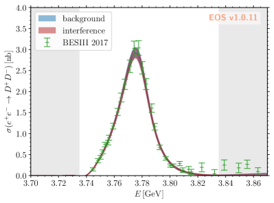
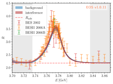
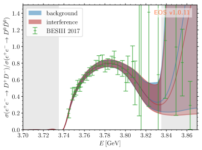
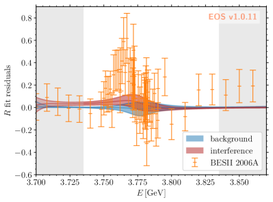
Figure 1: Predictions of our nominal (“background”) model for a couple of observables in the region of the $\psi(3770)$ resonance, compared to the experimental measurement performed by the BES experiment. Shaded areas are not used in the fit.
Top left: Cross-section of the $e^{+}e^{-}\to D^{+}D^{-}$ scattering. Top right: $R$-ratio. Bottom left: Ratio of the cross-sections of $e^{+}e^{-}\to D^{+}D^{-}$ and $e^{+}e^{-}\to D^{0}\bar{D}^{0}$. The experimental points are given for illustrative purpose and neglect the experimental correlations between the $D^{+}D^{-}$ and $D^{0}\bar{D}^{0}$ final states. Bottom right: Residuals of the fit of the $R$-ratio, the “background” model is used for the subtraction and compared with the “interference” model and experimental data.

Mass and width

Within both of our fit models, we obtain for the physical mass and total decay width of the $\psi(3770)$ identical results:

$$M_{\psi(3770)} =3777.1\pm 0.3\,\mathrm{MeV} \Gamma_{\psi(3770)} =26.3\pm 0.8\,\mathrm{MeV}\,.$$ ((24))

These values are fully consistent with those extracted in Ref. Coito:2017ppc

$$M_{\psi(3770)}^{\text{\cite[cite]{\@@bibref{Authors Phrase1YearPhrase2}{Coito:2017ppc}{\@@citephrase{(}}{\@@citephrase{)}}}}} =3777.0\pm 1.0\,\mathrm{MeV} \Gamma_{\psi(3770)}^{\text{\cite[cite]{\@@bibref{Authors Phrase1YearPhrase2}{Coito:2017ppc}{\@@citephrase{(}}{\@@citephrase{)}}}}} =24.6\pm 1.0\,\mathrm{MeV}\,.$$ ((25))

The stability of the pole location is very reassuring, given that there are significant differences in the actual modelling of the non-$\psi(3770)$ physics between our work and Ref. Coito:2017ppc , as outlined above.

We remind that our results are obtained from a $K$-matrix analysis. They are therefore not expected to reflect the parameters extracted from Breit-Wigner analyses, such as the one of Ref. Shamov:2016mxe or the world average quoted in the PDG review Workman:2022ynf . Nevertheless, we provide these respective results here for convenience

$$M_{\psi(3770)}^{\text{\cite[cite]{\@@bibref{Authors Phrase1YearPhrase2}{Shamov:2016mxe}{\@@citephrase{(}}{\@@citephrase{)}}}}} =3779.8\pm 0.6\,\mathrm{MeV} \Gamma_{\psi(3770)}^{\text{\cite[cite]{\@@bibref{Authors Phrase1YearPhrase2}{Shamov:2016mxe}{\@@citephrase{(}}{\@@citephrase{)}}}}} =25.8\pm 1.3\,\mathrm{MeV}\,.$$ ((26))

$$M_{\psi(3770)}^{\text{\cite[cite]{\@@bibref{Authors Phrase1YearPhrase2}{Workman:2022ynf}{\@@citephrase{(}}{\@@citephrase{)}}}}} =3778.1\pm 0.7\,\mathrm{MeV} \Gamma_{\psi(3770)}^{\text{\cite[cite]{\@@bibref{Authors Phrase1YearPhrase2}{Workman:2022ynf}{\@@citephrase{(}}{\@@citephrase{)}}}}} =27.5\pm 0.9\,\mathrm{MeV}\,.$$

We find the mass to be significantly lower than what is obtained in the literature. In contrast, we find the total decay width to be quite compatible with the literature. Given the variety of theoretical approaches to describe the data, we do not consider it meaningful to quote a statistical significance for the deviations.

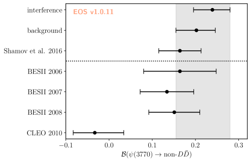
Figure 2: Comparison of our results for the branching ratio of the $\psi(3770)$ to $\textrm{non-}D\bar{D}$ final states with results from the phenomenological literature Shamov:2016mxe above the dotted line and the experimental literature BES:2008vad ; Ablikim:2007zz ; BES:2006fpf ; CLEO:2005mpm below. The grey band corresponds to our final result. Although they use different analysis techniques, the three results by the BESII experiment are not statistically independent.

Branching ratio of the $\psi(3770)$ to $\textrm{non-}D\bar{D}$

As already discussed in the literature Shamov:2016mxe ; BES:2008vad ; Ablikim:2007zz ; BES:2006fpf ; CLEO:2005mpm , the combined analysis of inclusive and exclusive measurements points to a substantial coupling of the $\psi(3770)$ to $\textrm{non-}D\bar{D}$ channels, i.e., yielding branching ratios $\mathcal{B}(\psi(3770)\to\textrm{non-}D\bar{D})$ at the level of a few percent. Our results for this branching ratio are presented in the last row of Tab.  1. We obtain

$$\mathcal{B}(\psi(3770)\to\textrm{non-}D\bar{D}) =(20.9\pm 4.5)\%$$ in the “background” model, ((27))

$$\mathcal{B}(\psi(3770)\to\textrm{non-}D\bar{D}) =(23.8\pm 4.3)\%$$ in the “interference” model. ((28))

As discussed above, these two results arise from two extreme analyses. We therefore expect the true value to be somewhat in between, and conclude that

$$\mathcal{B}(\psi(3770)\to\textrm{non-}D\bar{D})=(22\pm 6)\%$$ ((29))

is the most conservative presentation of our result. We compare our result to those quoted in the literature and find generally good statistical agreement. The most significant deviation at the $3\,\sigma$ level is seen in comparison to the CLEO results CLEO:2005mpm . However, it is noteworthy that our result is systematically larger than the previous determinations. We juxtapose those results with ours in Fig.  2.

We further investigate explicitly if such a coupling to the $\textrm{non-}D\bar{D}$ channel is required by the data. We do so by fitting a model “$\textrm{non-}D\bar{D}$” with vanishing bare couplings $g^{\psi(3770)}_{\text{eff(3770)}}=0$. As expected, we find that this model fits the data very poorly, with a low $p$-value of $10^{-4}$ and a Bayes factor $B(\text{``\cancel{$\textrm{non-}D\bar{D}$}''},\text{``background''})\simeq 10^{-6}$, substantially disfavouring this model with respect to our nominal fit models “background” and “interference”.

Isospin symmetry at the $\psi(3770)$ resonance

The $\psi(3770)$ resonance lies just above the $D^{0}\bar{D}^{0}$ threshold ($\sqrt{s}\sim 3.73\,\mathrm{GeV}$) and the $D^{+}D^{-}$ threshold ($\sqrt{s}\sim 3.74\,\mathrm{GeV}$). It is therefore sensitive to the differences in phase space volume between the two channels, leading to an apparent violation of isospin symmetry in the ratio of the exclusive cross sections; see the bottom left plot of Fig.  1 for an illustration. We prefer to probe the degree of isospin symmetry violation at hand of a quantity that is unaffected by these phase space effects. To this end, we investigate the ratio of the bare couplings between this resonance and either of the two channels. Unbroken isospin symmetry would yield unity, with symmetry breaking corrections being naturally suppressed by powers of $\alpha_{e}$ and $(m_{u}-m_{d})/m_{s}$.

We find the ratio of bare couplings to be

$$g_{D^{0}\bar{D}^{0}}^{\psi(3770)}/g_{D^{+}D^{-}}^{\psi(3770)}=1.00\pm 0.03\,,$$ ((30))

showing no sign of isospin symmetry violation in these decays in either model. We therefore conclude that the structure shown in the bottom plot of Fig.  1 originates from the difference in the phase space volumes. Our finding is in tension with findings in the literature Ishikawa:2023bnx ; Julin:2017jcl , which are obtained by fitting a Breit-Wigner-like line shape to the $\psi(3770)$ spectrum, but in line with the findings of Ref. Coito:2017ppc . In addition, we determine the isospin ratio of the bare $D\bar{D}$ couplings to the $\psi(2S)$ resonance to be $1.13\pm 0.13$, which is also compatible with unity with substantially larger uncertainties. The larger uncertainty obtained in this ratio is likely due to the fact that we are not fully modelling the $\psi(2S)$ resonance, as described in Sec.  2.1.

4 Summary and Outlook

In this paper we have performed a coupled-channel analysis of $e^{+}e^{-}\to\text{open charm}$ processes in a window around the $\psi(3770)$. Our analysis compares different models based on the $K$-matrix framework. We find that the now available high-resolution measurements by the BES, BESII, and BESIII experiments can be successfully described within our models. We further confirm through a Bayesian model comparison that the data require a sizable branching ratio to $\textrm{non-}D\bar{D}$ final states. Modelling these $\textrm{non-}D\bar{D}$ channels with a single effective $P$-wave channel, we obtain

$$\mathcal{B}(\psi(3770)\to\textrm{non-}D\bar{D})=(22\pm 6)\%\,.$$

Our result is compatible with but systematically larger than nearly all other determinations of this branching fraction. In recent years, various vector states were identified as good candidates for exotic states beyond the quark model—see Refs. Lebed:2016hpi ; Esposito:2016noz ; Olsen:2017bmm ; Guo:2017jvc ; Brambilla:2019esw ; Chen:2022asf for recent reviews. However, given our results we see no reason to question a dominant $\bar{c}c$ nature of the $\psi(3770)$. Note that hadronic loops that drive e.g. the emergence of hadronic molecules Guo:2017jvc are suppressed near threshold since they appear in a $P$-wave.

In the course of our analysis, we have struggled at times with the lack of statistical constraints on the electron couplings $g_{e^{+}e^{-}}^{r}$ . For this coupling to the $\psi(2S)$ we had to resort to external determinations of the partial width $\Gamma(\psi(2S)\to e^{+}e^{-})$. We would like to point out that this caveat could be overcome by using measurements of the cross section $e^{+}e^{-}\to\mu^{+}\mu^{-}$ in our phase space of interest, which are currently not available at the level of precision we require.

We look forward to future work in this field, where we plan to extend our analysis to larger values of $\sqrt{s}$ and, accordingly, to both additional channels and resonances. This extension will be essential for an envisaged phenomenological application: the transfer of the line shape information for the vector charmonia from measurements of $e^{+}e^{-}\to\text{hadrons}$ cross sections to theoretical predictions of exclusive $b\to s\ell^{+}\ell^{-}$ decays. A sketch of this application is provided in the appendix of this work. It is presently unclear if this application can be achieved without non-public information on the experimental measurements, and we hope that this work reinvigorates interest amongst our experimental colleagues.

Appendix A Relations to Non-local Form Factors in $\boldsymbol{b\to s\ell^{+}\ell^{-}}$

Non-local hadronic matrix elements in exclusive $b\to s\ell^{+}\ell^{-}$ processes pose a major source of systematic uncertainty to their theoretical predictions Gross:2022hyw . They have been the focus of theoretical developments for the past decade Khodjamirian:2010vf ; Khodjamirian:2012rm ; Jager:2012uw ; Ciuchini:2015qxb ; Bobeth:2017vxj ; Gubernari:2020eft ; Gubernari:2022hxn . Using $\bar{B}\to\bar{K}\ell^{+}\ell^{-}$ processes as an example for definiteness, a common definition of the dominant (charm-induced) non-local contributions reads

$$\mathcal{H}^{\mu}=i\!\int d^{4}x\,e^{iq\cdot x}\,\bra{\bar{K}(k)}T\big{\{}\bar{c}\gamma^{\mu}c(x),\sum_{i}C_{i}O_{i}(0)\big{\}}\ket{\bar{B}(q+k)}\,.$$ ((31))

Here the $O_{i}$ are local operators in the weak effective theory of mass dimension six and with flavour quantum numbers $sbcc$, and the $C_{i}$ are their respective Wilson coefficients. It is convenient to discuss this hadronic matrix element in terms of its scalar-valued non-local form factors

$$\mathcal{H}_{(\lambda)}(q^{2})=P^{\mu}(\lambda)\,\mathcal{H}_{\mu}(q)\,.$$ ((32))

Here $\lambda=0,\pm 1$ denotes a polarization state of the virtual photon coupling to the vector current, and $P^{\mu}(\lambda)$ are suitable projection operators; we refer to Ref. Gubernari:2022hxn for their definition. We emphasize that the $\mathcal{H}_{(\lambda)}$ are complex-valued functions even below all thresholds in $q^{2}$. This property emerges since the $\bar{B}$ meson can decay into an on-shell hadronic state by virtue of the four-quark operators $O_{i}$; see Ref. Khodjamirian:2010vf for a discussion on this topic.

A systematic approach to describing $\mathcal{H}_{(\lambda)}(q^{2})$ for $q^{2}<4M_{D}^{2}$ has been developed over the course of the last decade Bobeth:2017vxj ; Gubernari:2020eft ; Gubernari:2022hxn . Here, we instead focus on the open-charm region $q^{2}\geq 4M_{D}^{2}$. Common approaches to estimate or describe the non-local form factors in this region include an operator product expansion (OPE) of the time-ordered product in Eq.  (31) Grinstein:2004vb ; Beylich:2011aq , and a Breit-Wigner model of the broad charmonium resonance therein Kruger:1996cv ; Lyon:2014hpa ; Brass:2016efg . We propose a different approach based on the $P$-vector formalism that utilizes the information obtained in the main part of this work. First, we note that by crossing symmetry the scalar non-local form factors can be related to the scattering amplitude $\bar{B}K\to e^{+}e^{-}$

$$\mathcal{A}_{\bar{B}K,e^{+}e^{-}}\sim\sum_{\lambda}L_{\mu}P_{(\lambda)}^{*\mu}\mathcal{H}_{\lambda}\,,$$ ((33))

where $L_{\mu}=\bar{u}_{\ell}\gamma_{\mu}v_{\ell}$ denotes the leptonic current. Similarly, the $P$-wave amplitude for the processes $\bar{B}\to\bar{K}D\bar{D}$ can be related to $\bar{B}K\to D\bar{D}$ scattering amplitudes $\mathcal{A}_{\bar{B}K,D\bar{D}}$. Both of these processes are induced only by the weak interaction. As a consequence, their contributions to the overall width of the various vector charmonium resonances in the unitarization, for example through the $K$-matrix approach, are negligible. In such cases, the $P$-vector formalism provides a convenient approach to parametrize both of the amplitudes mentioned above:

$$\mathcal{A}_{\bar{B}K,a}=n_{a}\left[1-\mathcal{K}\Sigma\right]^{-1}P_{\bar{B}K}(s)\,.$$ ((34))

In the above $P_{\bar{B}K}$ represents the source term,

$$P_{\bar{B}K}(s)=\sum_{r}^{N_{R}}\frac{\alpha^{r}g^{r}_{\bar{B}K}}{m_{r}^{2}-s}+b_{\bar{B}K}\,$$ ((35))

split into a sum of the same resonances accounted for by the $K$-matrix and a background term $b_{\bar{B}K}$. As before, $m_{r}$ and $g_{r}$ represent bare masses and couplings, and the mass parameters should match those used in the $K$-matrix analysis. In contrast to the usual $P$-vector formalism, the couplings $g^{r}_{\bar{B}K}$ and the background term $b_{\bar{B}K}$ are complex-valued quantities. This can be readily understood from the fact that non-local form factors (and hence the scattering amplitudes) feature non-vanishing imaginary parts below all thresholds, as discussed above.

References

- (1) O. Bar and U.J. Wiese, Can one see the number of colors?, Nucl. Phys. B 609 (2001) 225 [hep-ph/0105258].
- (2) R.F. Lebed, R.E. Mitchell and E.S. Swanson, Heavy-Quark QCD Exotica, Prog. Part. Nucl. Phys. 93 (2017) 143 [1610.04528].
- (3) A. Esposito, A. Pilloni and A.D. Polosa, Multiquark Resonances, Phys. Rept. 668 (2017) 1 [1611.07920].
- (4) S.L. Olsen, T. Skwarnicki and D. Zieminska, Nonstandard heavy mesons and baryons: Experimental evidence, Rev. Mod. Phys. 90 (2018) 015003 [1708.04012].
- (5) F.-K. Guo, C. Hanhart, U.-G. Meißner, Q. Wang, Q. Zhao and B.-S. Zou, Hadronic molecules, Rev. Mod. Phys. 90 (2018) 015004 [1705.00141].
- (6) N. Brambilla, S. Eidelman, C. Hanhart, A. Nefediev, C.-P. Shen, C.E. Thomas et al., The states: experimental and theoretical status and perspectives, Phys. Rept. 873 (2020) 1 [1907.07583].
- (7) H.-X. Chen, W. Chen, X. Liu, Y.-R. Liu and S.-L. Zhu, An updated review of the new hadron states, Rept. Prog. Phys. 86 (2023) 026201 [2204.02649].
- (8) T. Aoyama et al., The anomalous magnetic moment of the muon in the Standard Model, Phys. Rept. 887 (2020) 1 [2006.04822].
- (9) A.G. Shamov and K.Y. Todyshev, Analysis of BaBar, Belle, BES-II, CLEO and KEDR data on line shape and determination of the resonance parameters, Phys. Lett. B 769 (2017) 187 [1610.02147].
- (10) Particle Data Group collaboration, Review of Particle Physics, PTEP 2022 (2022) 083C01.
- (11) T.V. Uglov, Y.S. Kalashnikova, A.V. Nefediev, G.V. Pakhlova and P.N. Pakhlov, Exclusive open-charm near-threshold cross sections in a coupled-channel approach, JETP Lett. 105 (2017) 1 [1611.07582].
- (12) S. Coito and F. Giacosa, Line-shape and poles of the , Nucl. Phys. A 981 (2019) 38 [1712.00969].
- (13) S.U. Chung, J. Brose, R. Hackmann, E. Klempt, S. Spanier and C. Strassburger, Partial wave analysis in K matrix formalism, Annalen Phys. 4 (1995) 404.
- (14) N.N. Achasov and G.N. Shestakov, Electronic width of the resonance interfering with the background, Phys. Rev. D 103 (2021) 076017 [2102.03738].
- (15) J.M. Blatt and V.F. Weisskopf, Theoretical nuclear physics, Springer, New York (1952), 10.1007/978-1-4612-9959-2.
- (16) BaBar collaboration, Study of the Exclusive Initial-State-Radiation Production of the System, 0710.1371.
- (17) Belle collaboration, Measurement of the near-threshold cross section using initial-state radiation, Phys. Rev. D77 (2008) 011103 [0708.0082].
- (18) BES collaboration, Measurements of the cross-section for at center-of-mass energies from 2 GeV to 5 GeV, Phys. Rev. Lett. 88 (2002) 101802 [hep-ex/0102003].
- (19) M. Ablikim et al., Measurements of the continuum R(uds) and R values in annihilation in the energy region between 3.650 and 3.872 GeV, Phys. Rev. Lett. 97 (2006) 262001 [hep-ex/0612054].
- (20) BESIII collaboration, Measurement of the Cross Section for Hadrons at Energies from 2.2324 to 3.6710 GeV, Phys. Rev. Lett. 128 (2022) 062004 [2112.11728].
- (21) CLEO collaboration, Measurement of Charm Production Cross Sections in Annihilation at Energies between 3.97 and 4.26 GeV, Phys. Rev. D80 (2009) 072001 [0801.3418].
- (22) BES collaboration, Measurements of the cross-sections for at 3.650 GeV, 3.6648 GeV, 3.773 GeV and the branching fraction for , Phys. Lett. B 641 (2006) 145 [hep-ex/0605105].
- (23) A.J. Julin, Measurement of Decays from the Resonance, Ph.D. thesis, Minnesota U., 2017.
- (24) R.V. Harlander and M. Steinhauser, rhad: A Program for the evaluation of the hadronic R ratio in the perturbative regime of QCD, Comput. Phys. Commun. 153 (2003) 244 [hep-ph/0212294].
- (25) EOS Authors collaboration, EOS: a software for flavor physics phenomenology, Eur. Phys. J. C 82 (2022) 569 [2111.15428].
- (26) D. van Dyk, M. Reboud, N. Gubernari, D. Leljak, P. Lüghausen, A. Kokulu et al., “EOS version 1.0.11 (to appear).”
- (27) E. Higson, W. Handley, M. Hobson and A. Lasenby, Dynamic nested sampling: an improved algorithm for parameter estimation and evidence calculation, Statistics and Computing 29 (2018) 891.
- (28) J.S. Speagle, dynesty: a dynamic nested sampling package for estimating Bayesian posteriors and evidences, Monthly Notices of the Royal Astronomical Society 493 (2020) 3132.
- (29) S. Koposov, J. Speagle, K. Barbary, G. Ashton, E. Bennett, J. Buchner et al., dynesty version 2.0.3, Dec., 2022. 10.5281/zenodo.7388523.
- (30) H. Jeffreys, The Theory of Probability, Oxford Classic Texts in the Physical Sciences, Oxford University Press (1939).
- (31) S. Weinberg, The Quantum theory of fields. Vol. 1: Foundations, Cambridge University Press (6, 2005), 10.1017/CBO9781139644167.
- (32) M. Ablikim et al., Anomalous Line Shape of the Cross Section for Hadrons in the Center-of-Mass Energy Region between 3.650 and 3.872 GeV, Phys. Rev. Lett. 101 (2008) 102004.
- (33) BES collaboration, Direct measurements of the cross sections for in the range from 3.65 GeV to 3.87 GeV and the branching fraction for , Phys. Lett. B 659 (2008) 74.
- (34) M. Ablikim et al., Direct measurements of the non- cross section at and the branching fraction for , Phys. Rev. D 76 (2007) 122002.
- (35) BES collaboration, Measurements of the branching fractions for , , and the resonance parameters of and , Phys. Rev. Lett. 97 (2006) 121801 [hep-ex/0605107].
- (36) CLEO collaboration, Measurement of at = 3773 MeV, Phys. Rev. Lett. 96 (2006) 092002 [1004.1358].
- (37) K. Ishikawa, O. Jinnouchi, K. Nishiwaki and K.-y. Oda, Wave-packet effects: a solution for isospin anomalies in vector-meson decay, Eur. Phys. J. C 83 (2023) 978 [2308.09933].
- (38) F. Gross et al., 50 Years of Quantum Chromodynamics, 2212.11107.
- (39) A. Khodjamirian, T. Mannel, A.A. Pivovarov and Y.M. Wang, Charm-loop effect in and , JHEP 09 (2010) 089 [1006.4945].
- (40) A. Khodjamirian, T. Mannel and Y.M. Wang, decay at large hadronic recoil, JHEP 02 (2013) 010 [1211.0234].
- (41) S. Jäger and J. Martin Camalich, On at small dilepton invariant mass, power corrections, and new physics, JHEP 05 (2013) 043 [1212.2263].
- (42) M. Ciuchini, M. Fedele, E. Franco, S. Mishima, A. Paul, L. Silvestrini et al., decays at large recoil in the Standard Model: a theoretical reappraisal, JHEP 06 (2016) 116 [1512.07157].
- (43) C. Bobeth, M. Chrzaszcz, D. van Dyk and J. Virto, Long-distance effects in from analyticity, Eur. Phys. J. C 78 (2018) 451 [1707.07305].
- (44) N. Gubernari, D. van Dyk and J. Virto, Non-local matrix elements in , JHEP 02 (2021) 088 [2011.09813].
- (45) N. Gubernari, M. Reboud, D. van Dyk and J. Virto, Improved theory predictions and global analysis of exclusive processes, JHEP 09 (2022) 133 [2206.03797].
- (46) B. Grinstein and D. Pirjol, Exclusive rare decays at low recoil: Controlling the long-distance effects, Phys. Rev. D 70 (2004) 114005 [hep-ph/0404250].
- (47) M. Beylich, G. Buchalla and T. Feldmann, Theory of decays at high : OPE and quark-hadron duality, Eur. Phys. J. C 71 (2011) 1635 [1101.5118].
- (48) F. Kruger and L.M. Sehgal, Lepton polarization in the decays and , Phys. Lett. B 380 (1996) 199 [hep-ph/9603237].
- (49) J. Lyon and R. Zwicky, Resonances gone topsy turvy - the charm of QCD or new physics in ?, 1406.0566.
- (50) S. Braß, G. Hiller and I. Nisandzic, Zooming in on decays at low recoil, Eur. Phys. J. C 77 (2017) 16 [1606.00775].