Constraining tensor-to-scalar ratio based on VLBI observations: PGWs induced-incoherence approach

Abstract

The background of primordial gravitational waves (PGWs) predicted by the inflationary scenario induce incoherence of the electromagnetic field propagating over cosmological distances. We propose a new schema to constrain the underlying inflationary parameters, in particular the tensor-to-scalar ratio r, based on angular size-redshift $\theta-z$ measurement accomplished by very long baseline interferometry (VLBI) surveys. VLBI observations rely on the van-Citter Zernike theorem, which expresses the coherence length of the emitted field in terms of its wavelength and angular size, i.e., $d_{\text{coh}}\leq\lambda/\theta$. In this study, we show that the interaction of the radio signal (involved in VLBI) with PGWs, along the propagation from a source located at redshift $z_{\ast}$ to the Earth, leads to the blurring of the visibility. The blurring effect is evaluated for the highly-squeezed PGW, where it turns out that in order not to ruin the visibility, the projected baseline of the interferometer must be smaller than $\xi_{\text{sq}}(z)$, which is inversely proportional to the the tensor-to-scalar ratio through $\xi_{\text{sq}}\propto\text{r}^{-1/2}$. Hence, VLBI observations based on interference pattern lead to a constraint on r imposed by the fact that $\xi_{\text{sq}}(z)$ is greater than $d_{coh}$ of the emitted radiation. In order to evaluate the constraint, we use a sample of compact radio quasars observed in VLBI and located at redshift range $0.46\leq z\leq 2.73$. We obtain a stringent upper-bound on the tensor-to-scalar ratio, $\text{r}<2\times 10^{-6}$, far beyond present constraints on this parameter. Further issues and caveats that potentially affect the results are reviewed. In particular, the possible effect of quantum-to-classical transition of PGWs is discussed. Ultimately, the background of primordial tensor perturbations may be more constrained with the help of the high-precision VLBI measurement of angular size-redshift of more distant sources.

1 Introduction

Interferometric methods have found vast applications in testing gravity either at the classical or quantum level. Starting from the famous Michelson-Morley interferometer to rule out the motion through “aether", light interferometry is now routinely used as a crucial technique to detect the tiniest effects of gravitational waves (GWs) with an incredible precision [1, 2, 3, 4, 5]. Whether these ripples in the spacetime obey quantum mechanical rules at a fundamental scale, say the Planck scale, is an open question and we lack any direct observational evidence in favor of that.

It is believed that space and time, when viewed at Planck scales, form a foam-like structure due to quantum fluctuations of the vacuum metric tensor [6, 7, 8]. Searching for Planck-scale quantum features of spacetime is an old quest, and many interferometric schemes based on the phase properties of electromagnetic (EM) radiation of distant objects have been proposed to inquire it [9, 10, 11, 12, 13, 14]. For instance, the phase interferometric approach early introduced in [10] inspects the Planck-scale physics through the spacetime foam-induced phase incoherence of light emitted from distant objects. In fact, it has been perceived that accumulation of tiny phase-incoherence during the long journey of light through the quantum fluctuations of the vacuum spacetime leads to loss of the phase of radiation at large distances. This approach was elaborated in [11] to rule out, or put stringent limits on some Planck-scale phenomenological models, by evidence of the diffraction pattern from the Hubble Space Telescope observations of SN 1994D and the unresolved appearance of a Hubble Deep Field galaxy at $z=5.34$. However, further studies [15] declared that such effects “are far below what is required in this approach to shed light on the foaminess of spacetime". Moreover, it was soon realized [16] that such an argument is only relevant for a division of amplitude interference such as occurs in a Michelson interferometer, whereas in a division of wavefront interference, such as in the stellar interferometry, the propagation of coherence is simply governed by the van-Citter Zernike theorem [17]. The former is connected to the notion of “temporal coherence" of a source, while the latter is relevant to its “spatial coherence", i.e., the phase correlations of the wavefronts at two points of space. It turned out that “spatial correlations are immune to any underlying fuzzy Planck scale", hence the Planck scale still remains inaccessible to interferometer detection with present technology [16]. Albeit, this result leaves the room for quantum gravitational effects of length scales much larger than the Planck length.

One important example is the relic background of quantum tensor perturbations naturally generated by the pumping engine of inflation; At the heart of cosmology, the inflationary scenario predicts that quantum fluctuations of the gravitational field present at the very early Universe have evolved and been amplified during the successive expansion of the Universe, and constitute a stochastic background of primordial gravitational waves (PGWs) today [18, 19, 20, 21, 22, 23, 24, 25, 26, 27, 28, 29, 30]. Due to its specific generating mechanism, PGWs spectrum span a full range of frequencies, corresponding to wavelengths much larger than the Planck scale. Thereupon, the quest for PGWs has made one of the main targets of today’s and upcoming GW detectors in different frequency bands: LIGO [31], Advanced LIGO [32, 33], VIRGO [34, 35], GEO [36, 37], AIGO [38, 39], LCGT [40], ET [41, 42] aiming at the frequency range $(10^{2}-10^{3})$ Hz; the space interferometers, such as the future LISA [43, 44] which is sensitive in the frequency range $(10^{-4}-10^{-1})$ Hz, BBO [45, 46, 47] and DECIGO [48, 49] both sensitive in frequency range $(0.1-10)$ Hz; and the pulsar timing arrays, including PPTA [50, 51, 52] and the planned SKA [53] working in frequency window $(10^{-9}-10^{-6})$ Hz. Besides, there are potential proposals able to detect the very-high-frequency part of PGWs, among which are the waveguide detector [54, 55, 56, 57], the proposed gaussian maser beam detector around GHz [58, 59, 60], and the $100$ MHz detector [61]. Moreover, the very low frequency portion of PGWs contribute to the anisotropy and polarization of cosmic microwave background (CMB) [62, 63, 64, 65, 66, 67, 68], yielding a magnetic-type polarization of CMB as a distinguished signal of PGWs, which would possibly be sensed by means of WMAP [69, 70, 71, 72, 73], Planck [74, 75], liteBIRD [76], the ground-based ACTPol [77] and the proposed CMBpol [78]. Detection of PGWs would not only confirm the inflationary scenario but also validate the quantum description of gravity at scales much larger than the Planck length.

In the present study, we introduce a new schema to search for the unique imprints of the PGWs on the spatial correlations of EM emission from furthest objects, and show how high-precision measurements of the angular size $\theta$ of distant objects using Very Long Baseline Interferometers (VLBI) exerts constraint on PGWs. The VLBI imaging technique takes advantage of the largest possible baselines (from several meters to thousands of kilometers) to precisely determine the location and fine structure of astronomical sources including Active Galactic Nucleis (AGNs) [79, 80, 81, 82, 83]. In a typical VLBI experiment, the incoming radiation of a distant source is collected by two or more spatially-separated telescopes (Fig. 1). Existence of spatial correlations throughout the baseline of the interferometer leads to the non-vanishing visibility pattern, which is used to determine the geometrical properties of the object, such as its angular diameter; Albeit this notion was first used in the Hanbury Brown and Twiss intensity interferometry to infer the angular diameter of Sirius A based on spatial correlations [84].

Noticeably, VLBI imaging has found great attention in constraining cosmology. For instance, the Event Horizon Telescope (EHT) which is a VLBI array imaging supermassive black holes (SMBHs) on event horizon scales, allows tests of deviation from general relativity by performing high precision measurements of the Kerr metric [85, 86]. Moreover, the Megamaser Cosmology Project (MCP) which is based on the VLBI sub-milliarcsecond angular mapping of compact objects, has provided an independent laboratory to constrain the Hubble constant, $H_{0}$, in parallel to other surveys such as CMB [87], likewise putting updated constraints on the mass of SMBHs [88]. In particular, capability of VLBI method in accurate measurement of the angular size-redshift ($\theta-z$) of intermediate-luminosity radio quasars has led to specify AGNs as astrophysical standard rulers with intrinsic size $\ell_{m}\sim 11.26$ pc, that can be used to constrain cosmological parameters, namely $H_{0},\Omega_{m},w_{\Lambda}$ [89, 90]. Recently, capability of the stellar interferometry as a potential tool to detect GWs in the lower frequency range $(10^{-6}-10^{-4})$ Hz is investigated [91]. However, to our best knowledge, VLBI measurements of the angular size-redshift has not yet been used to constrain the background of PGWs. Here, we promote the idea of employing stellar interferometric methods to constrain the underlying gravitational background of PGWs. We show how VLBI measurements of the angular size-redshift may put new constraint on the inflationary parameters, in particular the tensor-to-scalar ratio r.

It is worth mentioning that, in the literature there are numerous schema that focus on graviton-induced decoherence (GID) of light [92, 93] or particles [94, 95]. As a matter of fact, due to negligibly small coupling strength between gravity and radiation or matter fields, one usually needs a huge interaction time to observe the GID effect, provided that the system is completely isolated from other environmental effects that may lead to decoherence. In contrast, spatial correlations of a source are known to be immune to the typical environment induced-decoherence. In particular, van Citter-Zernike theorem implies that correlation length of initially spatial-incoherent sources grows with distance [17]. Hence, sources with cosmological distances that have had enough time to interact with the underlying gravitational background seem proper candidates to explore the underlying quantum gravitational effects.

The paper is organized as follows. Sec. 2 provides a brief introduction about the expansionary Universe, model parameters and PGWs. In Sec. 3, two-point correlation function of EM radiation is investigated and the coherence criteria is defined based on $\theta-z$ relation. Sec. 4 is devoted to further possible topics that can be addressed within the presented method. The paper is concluded in Sec. 5. A complete supplementary material containing derivation of the equations and its subtleties is provided in Appendices. (A,B,C). Throughout the paper, we occasionally take the speed of light unity, $c\equiv 1$, however it is sometimes explicitly written in specific expressions.

2 PGWs in expansionary Universe

2.1 Expansionary Universe

The spatially flat expanding Universe is often described by the Friedmann-Lemaître-Robertson-Walker (FLRW) metric and assumes a power-law scale factor $a(\eta)\propto\eta^{\alpha}$, where $\eta$ is the conformal time. Each successive expanding stage is specified with a different index $\alpha$. The whole expansion history can be regarded as [96]

$$a(\eta)=\begin{cases}\ell_{0}|\eta|^{1+\beta}\quad,\quad-\infty\leq\eta\leq\eta_{1}\\ a_{z}(\eta-\eta_{p})^{1+\beta_{s}}\quad,\quad\eta_{1}\leq\eta\leq\eta_{s}\\ a_{e}(\eta-\eta_{e})\quad,\quad\eta_{s}\leq\eta\leq\eta_{2}\\ a_{m}(\eta-\eta_{m})^{2}\quad,\quad\eta_{2}\leq\eta\leq\eta_{E}\\ \ell_{H}|\eta-\eta_{a}|^{-\gamma}\quad,\quad\eta_{E}\leq\eta\leq\eta_{H}\end{cases}$$ (2.1)

Usually the inflation index $\beta$ is related to the scalar spectral index of primordial perturbations according to $n_{s}=2\beta+5$ [21, 97, 98]. Basically, $n_{s}$ is a parameter introduced under the assumption that scalar perturbation spectrum obeys a power-law behaviour near the pivot scale $k_{0}$, with $n_{s}=1$ referred to Harrison-Zeldovich spectrum. The Planck2018 release favor $n_{s}\simeq 0.9649\pm 0.0044$ [99] (corresponding to $\beta\simeq-2.018\pm 0.0022$). However, the exact relation between $\beta$ and $n_{s}$ depends crucially on the specific inflationary potential through the (first order) slow-roll parameter $\epsilon_{V}$ (see Sec. 4.1). In this study, we generally consider $\beta$ as a free parameter of the model and, in some cases, we take $\beta=-2.0$ for the sake of illustration.

The parameter $\beta_{s}$ describes the expansion during the reheating stage starting right after the end of inflation, and may be related to the equation of state (EoS) parameter during the reheating stage $w_{reh}$, and to inflationary model parameters. In the literature, usually $\beta_{s}=1$ is chosen, which may correspond to a quadratic inflation potential with EoS parameter $w_{reh}=0$ [100, 101]. As discussed in Appendix. (A.2), $\beta_{s}$ affects only the high-frequency part of the PGWs spectrum, which leave a negligible effect on incoherence of the EM field. We mostly adopt the value $\beta_{s}=1$ in our investigations.

The parameter $\gamma$ determines the late expansion of the Universe governed by dark energy $\Lambda$. One may numerically solve the Friedmann equation with the ansatz Eq. (2.1) for given values of $\Omega_{\Lambda}$. For $\Omega_{\Lambda}\sim 0.7$ one has $\gamma\sim 1$ [102]. Throughout the paper we fix $\gamma=1$. The present scale factor is conveniently chosen $a(\eta_{0})=\ell_{H}$, so that the condition $|\eta_{0}-\eta_{a}|=1$ turns out. The constant $\ell_{H}$ is determined by $\ell_{H}=\gamma/H_{0}$ as a result of Eq. (2.1). Here, $H_{0}=100h\quad km/s/Mpc$ is the present Hubble constant with $h=0.6766$ being the Hubble constant in $km/s/Mpc$ unit [103]. Considering $\beta$ and $\beta_{s}$ as free parameters, there remain $12$ constants in Eq. (2.1), $8$ of which are reduced by the continuity of $a(\eta)$ and its derivative at four jointing points $\eta_{1}$, $\eta_{s}$, $\eta_{2}$ and $\eta_{E}$, resulting in $4$ independent parameters. One usually expresses these $4$ parameters in terms of increase of the scale factor during various stages, namely, $\zeta_{1}\equiv a(\eta_{s})/a(\eta_{1})$, $\zeta_{s}\equiv a(\eta_{2})/a(\eta_{s})$, $\zeta_{2}\equiv a(\eta_{E})/a(\eta_{2})$, and $\zeta_{E}\equiv a(\eta_{0})/a(\eta_{E})$. In our study, we take $\zeta_{E}=1.33$ and $\zeta_{2}=2547$. The increase of scale factor during the reheating and radiation-dominated stages, namely $\zeta_{1}$ and $\zeta_{s}$, generally depend on the reheating temperature $T_{reh}$ at which the radiation stage begins (see Appendix. A for details). Lower and upper bounds on $T_{reh}$ come from the Big Bang Nucleosynthesis (BBN) $T_{reh}\geq 10$ MeV and the energy scale at the end of inflation $T_{reh}\leq 10^{16}$ GeV, respectively. However, the CMB data modify the lower bound on the reheating temperature $T_{reh}\geq 6\times 10^{3}$ GeV [104], and gravitinos generation has given the upper bound $T_{reh}\leq 10^{7}$ GeV [105]. As discussed in Appendix. (A.2), $T_{reh}$ does not play significant roll in incoherence of the EM field, since it only changes the high-frequency part of the PGWs spectrum. However, the value of $T_{reh}$ could affect the range of other parameters, including $\beta,\beta_{s},\zeta_{1}$, when considering specific inflationary scenarios (see [106] for example). Here, we mainly adopt $T_{reh}=10^{8}$ GeV for the sake of illustration. The specific $T_{reh}$-dependency of $\zeta_{s}$ is given by Eq. (A.3), though $\zeta_{1}$ is usually regarded as a free parameter. So far, four parameters $(\beta,\beta_{s},T_{reh},\zeta_{1})$ determine the expansion of the Universe. The introduction of primordial perturbations adds extra degrees of freedom, namely $(A_{s,t},n_{s,t})$, among which we only treat $A_{t}$ or r as free parameter.

2.2 PGWs amplification in expanding Universe

PGWs originate from tensor perturbations of the FLRW metric. Started from the vacuum state, they have been amplified during the course of expansion of the Universe. It has been shown that the super-adiabatic amplification leads vacuum tensor perturbations to evolve into multi-mode highly squeezed state with enormously large number of gravitons [20, 21]. One may show that the squeezing spectrum at present, $e^{r_{k}}(\eta_{0})$, is related to the present perturbation field $h(k,\eta_{0})$ according to $e^{r_{k}}(\eta_{0})=\frac{1}{8\sqrt{\pi}\gamma}\frac{\ell_{H}}{\ell_{Pl}}\left(\frac{k_{H}}{k}\right)h(k,\eta_{0})$, given by (see Appendix. A.2)

$$e^{r_{k}}(\eta_{0})=\frac{1}{8\sqrt{\pi}}\frac{\ell_{H}}{\ell_{Pl}}\left(\frac{k_{H}}{k}\right)\begin{cases}A\left(\frac{k}{k_{H}}\right)^{2+\beta}\quad,\quad k\leq k_{E}\\ A\left(\frac{k}{k_{H}}\right)^{\beta-1}\frac{1}{(1+z_{E})^{3}}\quad,\quad k_{E}\leq k\leq k_{H}\\ A\left(\frac{k}{k_{H}}\right)^{\beta}\frac{1}{(1+z_{E})^{3}}\quad,\quad k_{H}\leq k\leq k_{2}\\ A\left(\frac{k}{k_{H}}\right)^{1+\beta}\left(\frac{k_{H}}{k_{2}}\right)\frac{1}{(1+z_{E})^{3}}\quad,\quad k_{2}\leq k\leq k_{s}\\ A\left(\frac{k}{k_{H}}\right)^{1+\beta-\beta_{s}}\left(\frac{k_{s}}{k_{H}}\right)\left(\frac{k_{H}}{k_{2}}\right)\frac{1}{(1+z_{E})^{3}}\quad,\quad k_{s}\leq k\leq k_{1}\\ \end{cases}$$ (2.2)

where the coefficient $A$ determines the initial perturbation amplitude that can be assessed by theoretical or observational normalization conditions. Here, $r_{k}$ stands for the squeezing amplitude of PGWs mode $k$. Characteristic wave numbers $k_{E},k_{H},k_{2},k_{s},k_{1}$ are determined once the increase parameters are fixed (see Appendix. A.2).

2.3 Quantum normalization condition (QNC)

Contribution of tensor perturbations around the pivot scale $k_{0}$ is usually expressed in terms of the so-called tensor-to-scalar ratio, $\text{r}_{k_{0}}\equiv\frac{\Delta_{h}^{2}(k_{0})}{\Delta_{\mathcal{R}}^{2}(k_{0})}$ with $\Delta_{h,\mathcal{R}}^{2}(k_{0})\equiv A_{t,s}$ being the tensor and scalar spectral amplitudes at the pivot scale $k_{0}$, respectively. We shall take $k_{0}=0.002Mpc^{-1}$ in our calculations. Basically, typical wavelength of tensor perturbations at the moment they exit the horizon during inflation must have been around the Hubble scale, hence much larger than the Planck length. Consequently, the perturbation field $h_{ij}$ at initial moment $\eta_{i}$ can be treated as a quantum field in its vacuum state, possessing an energy $\frac{1}{2}h\nu$. This assumption imposes a criteria on the initial amplitude $A$, called the quantum normalization condition (QNC) [20, 96, 107], so on the tensor-to-scalar ratio $\text{r}_{k_{0}}$. As a result of QNC, it can be shown that one ends up with the following theoretical constraint between the parameters ($\beta,\beta_{s},T_{reh},\zeta_{1},\text{r}$) [96],

$$A=\sqrt{A_{s}\text{r}}\left(\frac{k_{H}}{k_{0}}\right)^{\beta}\zeta_{E}^{\frac{2+\gamma}{\gamma}}=\frac{4}{c\sqrt{\pi}}\ell_{Pl}H_{0}\zeta_{1}^{\frac{\beta_{s}-\beta}{1+\beta_{s}}}\zeta_{s}^{-\beta}\zeta_{2}^{\frac{1-\beta}{2}}\zeta_{E}^{(1+\frac{1+\beta}{\gamma})}.$$ (2.3)

Upper bounds $A_{s}\lesssim 2.1\times 10^{-9}$ and $\text{r}_{0.002}<0.056$ has been made by Planck2018+ TT,TE,EE +lowE+lensing+BAO means [103]. However, here we treat r as a free parameter to be constrained by VLBI method, and express $\zeta_{1}$ as a function of other parameters,

$$\zeta_{1}(\beta,\beta_{s},T_{reh},\text{r})=\left(\frac{c\sqrt{\pi A_{s}\text{r}}}{4\ell_{Pl}H_{0}}\left(\frac{k_{H}}{k_{0}}\right)^{\beta}\zeta_{s}^{\beta}\zeta_{2}^{\frac{\beta-1}{2}}\zeta_{E}^{\frac{1-\beta}{\gamma}}\right)^{\frac{1+\beta_{s}}{\beta_{s}-\beta}}.$$ (2.4)

so that the expansionary model Eq. (2.1) is described by four independent parameters $(\beta,\beta_{s},T_{reh},\text{r})$. The strain field spectrum $h(k,\eta_{0})$ together with the corresponding squeezing factor $e^{r_{k}}(\eta_{0})$ are plotted in Fig. 4 for chosen values of $\beta=-2,\beta_{s}=1,T_{reh}=10^{8}GeV$ and $\text{r}=10^{-2}$. It can be seen that changing the reheating parameters only changes the high-frequency part of the spectrum, i.e., $k_{s},k_{1}$, which possess small squeezing.

3 PGWs induced incoherence of radiation

3.1 Two-point correlation function and spatial incoherence

The imprint of GWs on light is comprehensively studied in the literature, either at classical [30] or quantum level [108, 109, 92, 93]. In particular, it is shown that PGWs ruin the coherence properties of light after a characteristic time-scale $\tau_{gr}$ that crucially depends on the squeezing of the PGWs background, hence on the underlying inflationary model parameters [93]. However, as argued in [92] and [93], detection of such graviton induced-decoherence in a laboratory experiment seems challenging, mainly due to relatively small intrinsic coherence time of natural or artificial sources which are basically much tinier than the needed interaction time to have an observable effect.

To investigate the effect of PGWs background on EM field spatial correlations, we consider the general expression of two-point correlation function, defined by [17, 110]

$$\Gamma^{(1)}(\mathbf{r}_{1},t_{1};\mathbf{r}_{2},t_{2})\equiv\text{Re}\left[\Big{\langle}\hat{E}^{(-)}(\mathbf{r}_{1},t_{1})\hat{E}^{(+)}(\mathbf{r}_{2},t_{2})\Big{\rangle}\right].$$ (3.1)

where the expectation value is taken over $\hat{\rho}_{\text{em}}\otimes\hat{\rho}_{\text{pgws}}$. The field amplitudes $\hat{E}(\mathbf{r}_{i},t_{i})$ suffer the interaction with PGWs (in the Heisenberg picture). Basically, different light rays coming from two distant points of an extended emitter, say $\mathbf{k}$ and $\mathbf{k}^{\prime}$, travel along different paths, and the inhomogeneous nature of the GWs background leads them to experience nonidentical phase changes. This phase-incoherence mechanism is in competition with the growing phase-correlations that is established during the propagation of light as implied by the van Citter-Zernik theorem. The final result, however, drastically depends on the state of PGWs, $\hat{\rho}_{\text{pgws}}$.

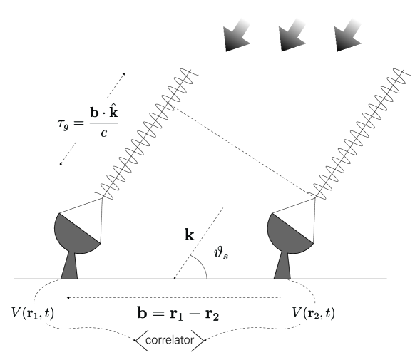
Figure 1: A two-telescope VLBI apparatus with distance $d_{12}=|\mathbf{r}_{1}-\mathbf{r}_{2}|$. The line of sight of the source makes angle $\vartheta_{s}$ with jointing line of the telescopes, which leads to a geometrical delay time $\tau_{g}=\mathbf{b}\cdot\hat{\mathbf{k}}/c$. Equal-time correlations $\langle V(\mathbf{r}_{1},t)V(\mathbf{r}_{2},t)\rangle$ are achieved by compensating for delay time $\tau_{g}$ [111].

To show that, one may consider a typical configuration of two-telescope interferometer, which could be the VLBI apparatus, as follows: two telescopes located at $\mathbf{r}_{1}$ and $\mathbf{r}_{2}$ collect the EM field rays $E(\mathbf{r}_{1},t_{1})$ and $E(\mathbf{r}_{2},t_{2})$, then the signals are correlated at zero time-difference so that the visibility $J(\mathbf{r}_{1},\mathbf{r}_{2})\equiv\Gamma^{(1)}(\mathbf{r}_{1},\mathbf{r}_{2};t,t)$ is obtained. The configuration of the system is depicted in Fig. (1). According to the van Citter-Zernik theorem, in the far zone and close to the direction normal to the source plane and parallel to it, the light produced by a spatially incoherent, quasi-monochromatic, uniform, circular source of radius $a$ is approximately coherent over a circular area $\Delta A$ whose diameter is $d_{12}\sim 2/(k_{0}\theta)$, where the angular size of the source is defined by $\theta\equiv 2a/D$ with $a$ and $D$ being the radius of the star and its distance to the Earth (see ch.4 of [17]). However, as it is shown in Appendix. (B.2), the presence of quantum GWs background appears as a modulating amplitude, $\mathcal{A}(\mathbf{r}_{1},t_{1};\mathbf{r}_{2},t_{2})$, defined by Eq. (B.8), which may completely spoil the interference pattern depending on the state of GWs, $\hat{\rho}_{\text{gws}}$.

In case of the so-called highly-squeezed PGWs specified by Eq. (2.2), it turns out that the induced phase-incoherence is such that spatial correlations vanish if $d_{12}\geq\xi_{\text{sq}}$ with $\xi_{\text{sq}}$ being a characteristic length-scale defined by Eq. (B.3.2). More precisely, the decaying envelope of the mutual intensity $J(\mathbf{r}_{1},\mathbf{r}_{2})$ turns out to be given by

$$\mathcal{A}(\theta;d_{12},z) = \exp\left(-\frac{d_{12}^{2}}{\xi_{\text{sq}}^{2}(\theta,z)}\right).$$ (3.2)

where $z$ is the redshift of the source. That is, PGWs background leads to the blurring of the visibility. The interference pattern survives if the detectors distance $d_{12}$ satisfy $\xi_{\text{sq}}\gtrsim d_{12}$. Nevertheless, successful measurement of the angular size $\theta$ of distant objects based on visibility implies that the correlation length of the source is at least equal to the projected baseline of the VLBI instrument, say $b\sin\vartheta_{s}=d_{12}\sin\vartheta_{s}\sim 2/(k_{0}\theta)$, otherwise the VLBI apparatus could not be able to resolve the source. In the following, without lose of generality we consider the case of normal incidence, where $\vartheta_{s}=90^{\circ}$. In practical situation of VLBI experiments the geometrical delay time $\tau_{g}$ arising from asymmetric configuration of the instrument with respect to the line of sight of the source is usually compensated, so that equal-time correlation of EM signals $\langle V(\mathbf{r}_{1},t)V(\mathbf{r}_{2},t)\rangle$ is achieved [111]. Hence, one may regard the separation length $d_{12}\equiv d_{\text{coh}}\equiv 2/(k_{0}\theta)$ as a threshold of coherence and the coherence criteria $\xi_{\text{sq}}\gtrsim d_{12}$ becomes $\xi_{\text{sq}}\gtrsim d_{\text{coh}}$. It seems easier to work with the dimensionless coherence parameter defined by $\alpha_{\text{coh}}\equiv\log(k_{0}d_{\text{coh}})$ and the gravitational induced incoherence parameter $\alpha_{\text{sq}}\equiv\log(k_{0}\xi_{\text{sq}})$; The criteria of non-vanishing visibility implies that $\alpha_{\text{sq}}\gtrsim\alpha_{\text{coh}}$. In the following, we use the $\theta-z$ data measured by VLBI means to find the threshold coherence parameter $\alpha_{\text{coh}}(z)=\log(2/\theta(z))$ and constrain $\alpha_{\text{sq}}(z)$ based on that.

3.2 Definition of the fiducial $\Lambda$CDM coherence parameter $\alpha_{\text{fid}}$ based on VLBI measurement of angular size-redshift $\theta-z$

Here we make use of a sample of 120 radio-quasars described in [89] with redshift range between $z=0.462$ and $z=2.73$, chosen from a well-known $2.29$ GHz VLBI survey called P85 [112]. These 120 radio quasars have been carefully selected for cosmological studies [89, 90, 113]. The scatter diagram of the observed angular size for 120 radio quasars is shown in Fig. 2. Detailed information about angular size $\theta(z)$ and redshift $z$ data are listed in Table. 1 of Cao et al [89].

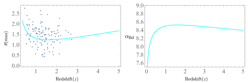
Figure 2: Left panel: The scatter plot of angular sizes of 120 compact radio quasars. The cyan line denotes the angular size $\theta(z)$ calculated from the fiducial flat $\Lambda$CDM model ($H_{0}=70.0km/s/Mpc,\Omega_{m}=0.3$) [90]. Right panel: The fiducial flat $\Lambda$CDM coherence parameter defined by $\alpha_{\text{fid}}\equiv\log(2/\theta_{\text{fid}}(z))$. The criteria $\alpha_{\text{sq}}\gtrsim\alpha_{\text{fid}}$ is used to constrain the gravitational-induced incoherence.

The angular size-redshift relation in the flat $\Lambda$CDM model is encapsulated in $\theta(z)=\ell_{m}H_{0}(1+z)[\int_{0}^{z}dz^{\prime}/\sqrt{\Omega_{m}(1+z^{\prime})^{3}+(1-\Omega_{m})}]^{-1}$ [114] where the best fit to data is found to be given by $\Omega_{m}=0.3$ with $\ell_{m}=11.26$pc [90]. The right panel in Fig. (1) shows the fiducial flat $\Lambda$CDM coherence parameter $\alpha_{\text{fid}}(z)=\log(2/\theta_{\text{fid}}(z))$ for $\Omega_{m}=0.3$ and $\ell_{m}=11.26$pc. In next section, we use the coherence criteria $\alpha_{\text{fid}}(z)\lesssim\alpha_{\text{sq}}(z)$ to constrain the tensor-to-scalar ratio of highly-squeezed PGWs.

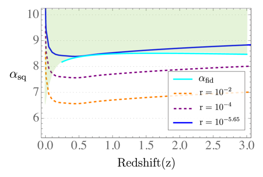
Figure 3: The coherence parameter $\alpha_{\text{sq}}$ versus redshift $z$ based on numerical calculations. The cyan curve shows $\alpha_{\text{fid}}=\log(2/\theta_{\text{fid}})$ calculated based on the fiducial flat $\Lambda$CDM model for $\Omega_{m}=0.3$. Dashed orange and purple curves correspond to $\alpha_{\text{sq}}$ for $\text{r}=10^{-2}$ and $\text{r}=10^{-4}$, respectively. The green region shows the coherence criteria $\alpha_{\text{fid}}\geq\alpha_{\text{sq}}$ fulfilled. The coherence criteria is violated for $\text{r}\gtrsim 10^{-5.65}$ shown by the blue curve. This determines the highest allowed value of r so that the coherence criteria if fulfilled. Here, $\beta=-2.0$, $\beta_{s}=1$ and $T_{reh}=10^{8}$ GeV are chosen. Hence the coherence criteria implies the upper-bound $\text{r}\lesssim 10^{-5.65}\simeq 2.24\times 10^{-6}$.

3.3 $\alpha_{\text{fid}}(z)$ versus $\alpha_{\text{sq}}(z)$: constraint on the tensor-to-scalar ratio r

In expression of Eq. (3.2), the implicit dependence of the incoherence length $\xi_{\text{sq}}(z,\theta)$ on the model parameters $(\beta,\beta_{s},\zeta_{1},T_{reh},\text{r})$ is encapsulated in the squeezing factor $e^{r_{k}}$ given by Eq. (2.2). The behaviour of the incoherence parameter $\alpha_{\text{sq}}$ versus redshift $z$ is shown in Fig. (3) for different values of r where $\beta$ is fixed to $\beta=-2.0$, $\beta_{s}=1$ and $T_{reh}=10^{8}$ GeV are chosen: orange and purple dashed curves correspond to $\text{r}=10^{-2}$, $10^{-4}$, respectively and the cyan line shows the coherence threshold $\alpha_{\text{fid}}=\log(2/\theta)$ implied by VLBI observations. The blue curve corresponds to $\text{r}=10^{-5.65}\simeq 2.24\times 10^{-6}$. The incoherence parameter $\alpha_{\text{sq}}$ is a quantity independent from the EM frequency of the emitted light, while sensitively dependent on the initial amplitude of PGWs, encapsulated in r. Increasing or decreasing r shifts the curves down or up as a result of increasing or decreasing the strain field and squeezing factor, that in turn strengthens or attenuates the incoherence mechanism (Note that decreasing in $\alpha_{\text{sq}}$ means decreasing in $\xi_{\text{sq}}$ hence a more severe effect). Basically, from Eq. (B.3.2) one may deduce that $\xi_{gr}\propto\text{r}^{-1/2}$. Moreover, it can be seen that changing $\beta$ shifts the curves slightly up or down, while changing $\beta_{s}$ and $T_{reh}$ practically do not leave a sensible effect on the incoherence parameter.

It is seen from Fig. 3 that coherence criteria is fulfilled for tensor-to-scalar ratio as small as $\text{r}\lesssim 10^{-5.65}$ when $\beta=-2.0$. This small value for r is more stringent than (although compatible with) the threshold value $\text{r}=10^{-3}$ sensible by Planck Means, and is below the constraining power of post-Planck CMB missions [115]. Although this upper-bound on r is obtained independent from the specific inflationary model, one could apply the present schema to given inflationary models. In next section, general implications of the upper-bound $\text{r}\lesssim 10^{-5.65}$ on the slow-roll parameters $\epsilon_{V}$ and $n_{t}$ are investigated. Moreover, the hypothesis of PGWs being in the highly-squeezed vacuum state is inquired in detail where further issues are addressed.

4 Discussion and conclusions

4.1 Implications for the slow-roll framework

We have seen that PGWs induced-incoherence may put constraint on the inflationary parameter r under the quantum normalization condition, while the reheating parameters such as $(\beta_{s},\zeta_{1},T_{reh})$ are not sensible by this method as described before. Although we have presented the method in a model-independent manner, specific models describing the inflationary epoch can be addressed straightforwardly; General inflationary parameters such as $\text{r},\beta,n_{s},n_{T}$ are expressible in terms of the slow-roll parameters within a given inflationary model with specific potential $V(\phi)$. Hence, the coherence criteria based on $\theta-z$ observations may put constraint on the model parameters. However, the stringent upper-bound $\text{r}\lesssim 10^{-5.65}$ which was obtained model-independently holds on, and implies extremely small values for the (first order) slow-roll parameter $\epsilon_{V}$.

Generally, under the first order slow-roll approximation, tensor and scalar spectral tilts are determined by $n_{t}\simeq-2\epsilon_{V}$ and $n_{s}-1\simeq 2\eta_{V}-6\epsilon_{V}$, where $\epsilon_{V}$ and $\eta_{V}$ are the slow-roll parameters which depend on the specific form of the inflationary potential $V(\phi)$. Taking the initial tensor spectrum $h(k_{0},\eta_{i})=A(k_{0}/k_{H})^{2+\beta}$ to constitute tensor perturbation spectrum at pivot scale $\Delta_{t}^{2}(k_{0})$, one obtains the relation $n_{t}=2\beta+4$ [106]. Hence, a general (model-independent) results is the relation between $\epsilon_{V}$ and $\beta$ given by $\epsilon_{V}=-\beta-2$. Note that, according to definition $\epsilon_{V}>0$ so that $\beta<-2$. Moreover, the single-field slow-roll inflation predicts $\text{r}=-8n_{t}=16\epsilon_{V}=-16(\beta+2)$. Assuming $\text{r}\lesssim 10^{-5.65}$ implies an upper-bound on the slow-roll parameter $\epsilon_{V}\lesssim 1.4\times 10^{-7}$ and the tensor spectral index $|n_{t}|\lesssim 2.8\times 10^{-7}$. Such small values for r and $\epsilon_{V}$ are compatible with prediction of some specific inflationary models [115]. Hence, knowledge of upper-bounds on slow-roll parameters based on VLBI method may rule out inflationary models or put stringent constraint on the model parameters.

4.2 Remarks on the assumption of quantum normalization condition

Throughout the paper, we considered QNC that exerts a specific relation between different parameters as implied by Eq. (2.3). Although it seems natural to assume that PGWs modes were in vacuum state before they exit the horizon, the vacuum state can not be defined unambiguously due to the particle creation in the expanding Universe [116]. If one disregard QNC, the only normalization of tensor spectrum could be obtained from the definition $\text{r}\equiv\frac{\Delta_{h}^{2}(k_{0})}{\Delta_{\mathcal{R}}^{2}(k_{0})}$. For $k_{H}\leq k_{0}\leq k_{2}$, Eq. (22) of [96] yields $h(k_{0},\eta_{0})=A\left(k_{0}/k_{H}\right)^{\beta}\zeta_{E}^{-3}=[\Delta_{h}^{2}(k_{0})]^{1/2}=[\Delta_{\mathcal{R}}^{2}(k_{0})\text{r}]^{1/2}$, and the constraint on the initial amplitude $A$ outcomes as $A=\sqrt{A_{s}\text{r}}\left(k_{H}/k_{0}\right)^{\beta}\zeta_{E}^{3}$, as is given by the left hand-side of Eq. (2.3). Consequently, the parameters $\zeta_{1}$ which was related to $\beta,\beta_{s}$ and $T_{reh}$ becomes a free parameter, taking a broad range of values $\zeta_{1}\in(10^{0},10^{16})$ [96]. In any case, $\zeta_{1}$ is the increase of the scale factor during reheating which merely determines the highest PGWs mode $k_{1}$ according to Eq. (A.4). This part of the spectrum practically doesn’t leave observable effect on the correlations of light, due to negligibly small strain field. In this regard, the final results Eq. (B.3.2, B.25, B.3.2) are not sensitive to the QNC assumption.

4.3 Remarks on the squeezed nature of PGWs and quantum-to-classical transition issue

The longstanding issue of the quantum-to-classical transition of inflationary perturbations has been widely scrutinized in the literature [117, 118, 119, 120, 121]. As a general result of interaction with environment, PGWs modes lose their quantum coherence. Consequently, the present state of the PGWs background is not a pure squeezed state in its rigid sense. However, the standard predictions for the rms values of the perturbations generated during inflation are not affected by these mechanisms, at least for scales of interest in cosmological applications [117]. Specially, it is shown that gravitons are robust against the decoherence caused by the cosmological magnetic fields and the squeezing of PGWs is not spoiled [122]. On the other hand, it is argued that, for the scales probed in the CMB, decoherence is effective as soon as inflation proceeds above $\sim 5\times 10^{9}$ GeV, and if inflation proceeds at GUT scale, decoherence is incomplete only for the scales crossing out the Hubble radius in the last $\sim 13$ $\mathrm{e}-$folds of inflation, namely the high-frequency part of PGWs [123]. By all means, the decay rate of coherence of PGWs depends crucially on the specific form of the interaction Hamiltonian, as investigated in [118]. In generic case, the final state of the PGWs, $\hat{\rho}_{\text{pgws}}(\eta_{0})$, can be considered as a mixture of different quantum and classical states, namely the vacuum state (associated to those modes which were outside the horizon for ever), coherent, squeezed and thermal states. This crucially affects the phase incoherence process and the resulting interference pattern, through the quantity $\mathcal{A}_{\mathbf{k}}(\mathbf{r}_{1},t_{1};\mathbf{r}_{2},t_{2})$ defined by Eq. (B.8) which depends explicitly on the PGWs state $\hat{\rho}_{\text{pgws}}$. To better grasp the distinction between different PGWs states in spatial interference of the EM field, one may consider the effect of GWs continuum in vacuum, coherent and thermal states, on phase coherence.

Vacuum perturbations of GWs field can be described by the density matrix $\hat{\rho}_{\text{vac}}=\prod_{K}|0_{K}\rangle\langle 0_{K}|$ with $K=(\mathbf{K},\gamma)$ denoting the GWs modes. From Eq. (B.8), the modulation amplitude $\mathcal{A}(\mathbf{r}_{1},t_{1};\mathbf{r}_{2},t_{2})$ become

$$\mathcal{A}_{\text{vac}}(\mathbf{r}_{1},t_{1};\mathbf{r}_{2},t_{2}) = \underbrace{e^{i\int d^{3}K\kappa_{K}^{2}\Im[\eta^{\ast}(\mathbf{r}_{1},t_{1})\eta(\mathbf{r}_{2},t_{2})]}}_{\text{coherent oscillations}}\underbrace{e^{-\frac{1}{2}\int d^{3}K\kappa_{K}^{2}\big{|}\eta(\mathbf{r}_{1},t_{1})-\eta(\mathbf{r}_{2},t_{2})\big{|}^{2}}}_{\text{incoherent decay}},$$ (4.1)

that means, vacuum perturbations of GWs field induce coherent oscillations of the interference phase, accompanied by destruction of the visibility amplitude. However, both effects are quadratic in $(\hbar\omega_{0}/E_{Pl})$ that makes it impossible to witness any observable effect. For a coherent background, one may describe the state of GWs by density matrix $\hat{\rho}_{\text{coh}}=\prod_{K}|\beta_{K}\rangle\langle\beta_{K}|$ with $\beta_{K}$ being the corresponding coherence parameter of mode $K=(\mathbf{K},\gamma)$. One can consider the polar representation $\beta_{K}=\bar{n}_{K}^{1/2}e^{i\theta_{\beta_{K}}}$ with $(\bar{n}_{K},\theta_{\beta_{K}})$ being the mean number of gravitons in the coherent state $|\beta_{K}\rangle$ and the coherence phase, respectively. In this case, the modulation amplitude $\mathcal{A}_{\mathbf{K}}(\mathbf{r}_{1},t_{1};\mathbf{r}_{2},t_{2})$ Eq. (B.8) turns out

$$\mathcal{A}_{\text{coh}}(\mathbf{r}_{1},t_{1};\mathbf{r}_{2},t_{2}) = \mathcal{A}_{\text{vac}}(\mathbf{r}_{1},t_{1};\mathbf{r}_{2},t_{2})\underbrace{e^{i\mathcal{N}(\mathbf{r}_{1},t_{1};\mathbf{r}_{2},t_{2})}}_{\text{coherent oscillations}},$$ (4.2)

where $\mathcal{N}(\mathbf{r}_{1},t_{1};\mathbf{r}_{2},t_{2})=2\int d^{3}K\kappa_{K}\Im\left[\eta(\mathbf{r}_{1},t_{1})-\eta(\mathbf{r}_{2},t_{2})\right]\beta^{\ast}_{K}$. Hence, in addition to the same behaviour induced by vacuum perturbation field, gravitons in the coherent state induce additional coherent phase oscillations in the interference pattern that is proportional to the coherence parameter $\beta_{K}$. This effect is first-order in $(\hbar\omega_{0}/E_{Pl})$ and may get amplified in the presence of high-intensity coherent state of gravitons. Indeed, the effect of a coherent background may be searched through the phase modulation term $\cos[\mathbf{k}\cdot(\mathbf{r}_{1}-\mathbf{r_{2}})+\mathcal{N}(\mathbf{r}_{1},t_{1};\mathbf{r}_{2},t_{2})]$ present in the interference pattern (see Sec. B.2), provided that the mean number of gravitons per mode $\bar{n}_{K}$ is so high that compensate the insignificant prefactor $\hbar\omega_{0}/E_{Pl}$. For the visible light with frequency $\sim 10^{15}$ Hz, one needs $\bar{n}_{K}^{1/2}\gtrsim 10^{29}$ for a meaningful change in the EM phase.

In case of thermal gravitons with mean graviton number per mode $\bar{n}_{\text{th}}(K)$, one may describe the GWs state by $\hat{\rho}_{\text{th}}=\prod_{K}\hat{\rho}_{\text{th}_{K}}$ and find the modulation amplitude as

$$\mathcal{A}_{\text{th}}(\mathbf{r}_{1},t_{1};\mathbf{r}_{2},t_{2}) = \mathcal{A}_{\text{vac}}(\mathbf{r}_{1},t_{1};\mathbf{r}_{2},t_{2})\underbrace{e^{-\int d^{3}K\kappa_{K}^{2}\bar{n}_{\text{th}}(K)\big{|}\eta(\mathbf{r}_{1},t_{1})-\eta(\mathbf{r}_{2},t_{2})\big{|}^{2}}}_{\text{contribution of thermal gravitons}},$$ (4.3)

i.e., mean number of thermal gravitons induce phase incoherence. To conclude the comparison between different states of gravitons, it is worthy to review the case of squeezed GWs. Following the discussion in Appendix. (B), the modulation amplitude Eq. (B.10) and Eq. (B.2) can be rewritten as

$$\mathcal{A}_{\text{sq}}(\mathbf{r}_{1},t_{1};\mathbf{r}_{2},t_{2}) = \mathcal{A}_{\text{vac}}(\mathbf{r}_{1},t_{1};\mathbf{r}_{2},t_{2})\underbrace{e^{-\int d^{3}K\kappa_{K}^{2}\bar{n}_{sq}(K)|\eta(\mathbf{r}_{1},t_{1})-\eta(\mathbf{r}_{2},t_{2})|^{2}}}_{\text{contribution of mean number of gravitons}}$$ (4.4)

$$\times \underbrace{e^{-\int d^{3}K\kappa_{K}^{2}\sinh r_{K}\cosh r_{K}\Re\left[e^{-i\theta_{K}}\left(\eta(\mathbf{r}_{1},t_{1})-\eta(\mathbf{r}_{2},t_{2})\right)^{2}\right]}}_{\text{contribution of quantum correlations}},$$

where the contribution of mean number of squeezed graviton $\bar{n}_{sq}(K)$ and the contribution of the correlations of type $\langle\hat{b}_{K}\hat{b}_{K}\rangle_{\hat{\rho}_{\text{sq}}}$ in the incoherence mechanism are written separately. Although mean number of gravitons in thermal and squeezed states act similarly, the presence of quantum correlations between gravitons in the squeezed state develop different behaviour. The substantial difference between thermal and squeezed gravitons emerges as a result of quantum correlations in the squeezed state, that are absent in thermal state. To see that, one may perform calculations similar to steps described in Appendix. (B) for squeezed state, to find the incoherence length induced by thermal gravitons $\hat{\rho}_{\text{th}}$. In this case, the modulation amplitude Eq. (4.3) can be rewritten as

$$\mathcal{A}_{\text{th}}(\mathbf{r}_{1},t_{1};\mathbf{r}_{2},t_{2}) \equiv e^{-\mathcal{B}_{\text{th}}(\mathbf{r}_{1},t_{1};\mathbf{r}_{2},t_{2})},$$ (4.5)

where the vacuum contribution is disregarded and the function

$$\mathcal{B}_{\text{th}}(\mathbf{r}_{1},t_{1};\mathbf{r}_{2},t_{2}) = \frac{1}{(4\pi)^{2}}\left(\frac{\hbar\omega_{0}}{E_{Pl}}\right)^{2}\int d\Phi_{K}d(\cos\Theta_{K})F_{\gamma}^{2}(\hat{\mathbf{K}},\hat{\mathbf{k}})$$

$$\times \int\frac{dK}{K}\bar{n}_{\text{th}}(K)\left(4\sin^{2}\left[\frac{\Omega_{K}}{2}(t_{1}-t_{2}+\frac{d_{12}}{c}\sin\Theta_{K})\right]\right)$$

$$= \bigg{(}\frac{1}{(4\pi)^{2}}\left(\frac{\hbar\omega_{0}}{E_{Pl}}\right)^{2}\int d\Phi_{K}d(\cos\Theta_{K})F_{\gamma}^{2}(\hat{\mathbf{K}},\hat{\mathbf{k}})\sin\Theta_{K}^{2}\int dKK\bar{n}_{\text{th}}(K)\bigg{)}d_{12}^{2}$$

$$= \xi_{\text{th}}^{-2}d_{12}^{2},$$

accounts for the decaying behaviour. In the second line of Eq. (4.3), Eqs. (B.18,B.19) are used and thermal induced incoherence length $\xi_{\text{th}}$ is defined by

$$\xi_{\text{th}}^{-2} = \frac{1}{(4\pi)^{2}}\left(\frac{\hbar\omega_{0}}{E_{Pl}}\right)^{2}\int d\Phi_{K}d(\cos\Theta_{K})F_{\gamma}^{2}(\hat{\mathbf{K}},\hat{\mathbf{k}})\sin\Theta_{K}^{2}\int dKK\bar{n}_{\text{th}}(K).$$ (4.7)

$\xi_{\text{th}}$ depends on the mean number of thermal gravitons while does not depend on the interaction time $t_{\text{int}}$ between source emission and detector receiver. In other words, since the signals coming from two distant edges of the source spend roughly equal time to reach to the Earth, $t_{1}=t_{2}\sim D/c$, the time difference $t_{1}-t_{2}$ would be zero. This is in contrast to the case of squeezed GWs background where the contribution of quantum correlations leads to time-dependent decaying behaviour, as can be seen from Eq. (B.3.2). In fact, Eq. (B.3.2) for $\xi_{\text{sq}}$ can be evidently separated to two part,

$$\xi_{\text{sq}}^{-2} = \frac{1}{(4\pi)^{2}}\left(\frac{\hbar\omega_{0}}{E_{Pl}}\right)^{2}\int d\Phi_{K}d(\cos\Theta_{K})F_{\gamma}^{2}(\hat{\mathbf{K}},\hat{\mathbf{k}})\sin\Theta_{K}^{2}$$ (4.8)

$$\times \int KdK\Big{(}\bar{n}_{\text{sq}}(K)-\frac{1}{2}\sinh(2r_{k})\cos\Big{[}2\Omega_{K}t_{\text{int}}(1-\cos\Theta_{K})\Big{]}\Big{)},$$

the first term is constant and related to the mean number of gravitons, while the second term is non-stationary and comes from correlations between gravitons in the squeezed state. Indeed, as noted by L. P. Grishchuk [20], non-stationary nature of the squeezed background is a consequence of squeezing and severe reduction of the phase uncertainty, and is directly reflected in the non-stationary behaviour of the spectral variance $\langle h^{2}(k,\eta_{0})$ of the PGWs field. Here, the phase correlations between gravitons in the squeezed state lead to non-stationary behaviour of the decaying amplitude. Consequently, time-dependence, or equivalently, redshift-dependence of the correlation length $\xi_{\text{sq}}$ can be regarded as a characteristic feature of the squeezed background.

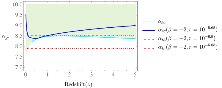
Figure 4: Comparison between thermal and squeezed induced incoherence. The cyan and blue curves show the fiducial flat $\Lambda$CDM coherence parameter $\alpha_{\text{fid}}$ and squeezed induced incoherence parameter $\alpha_{\text{sq}}$ for $\text{r}=10^{-5.65}$, respectively. The red and gray dot-dashed lines correspond to $\alpha_{\text{th}}$ for $\text{r}=10^{-5.65}$ and $\text{r}=10^{-6.9}$, respectively. The green region shows the region that coherence criteria $\alpha_{\text{gr}}\geq\alpha_{\text{fid}}$ is fulfilled.

Fig. 4 shows the comparison between thermal and squeezed incoherence parameters versus the redshift, where both states occupy the same mean number of gravitons $\bar{n}_{\text{th}}(K)=\bar{n}_{\text{sq}}(K)=\sinh^{2}r_{K}\sim e^{2r_{K}}/4$ implied by Eq. (2.2). The cyan curve shows the coherence parameter $\alpha_{\text{fid}}$ implied by the fiducial flat $\Lambda$CDM model. The red and gray dot-dashed lines correspond to $\alpha_{\text{th}}$ for $\text{r}=10^{-5.65}$ and $\text{r}=10^{-6.9}$ respectively, while the blue curve corresponds to $\alpha_{\text{sq}}$ for $\text{r}=10^{-5.65}$. Hence, at large enough distances where $t_{1}\sim t_{2}$, mean number of gravitons in thermal or squeezed state act as a stationary medium that induces a constant reduction of phase-correlations, that only depends on the PGWs amplitudes through r. On the other hand, quantum correlations between gravitons in the squeezed state induce a non-stationary behaviour of the incoherence parameter, as reflected in the $z-$dependence of $\alpha_{\text{sq}}$, which tends to relieve the incoherence mechanism. That is, for a given r, thermal gravitons leave a more severe effect than a squeezed state with the same mean number of gravitons. In the worst scenario that PGWs have been thermalized as a result of quantum-to-classical transition, the coherence criteria leads to the upper-bound $\text{r}=10^{-6.9}$, which is around 100 times smaller than the prediction of $\text{r}=10^{-5.65}$ for pure squeezed PGWs. In this case, one has an upper bound on the late value of the tensor-to-scalar ratio, since the decoherence induced by environment after the generation of PGWs during inflationary stage has lead the correlations between gravitons to decay. We conclude this section by summing up the results as following:

1. Vacuum fluctuations of the GWs field induce coherent (non-dissipative) oscillations as well as decaying behaviour in the phase correlations of EM field, though not sensible due to negligible effect.

2. GWs background in coherent state, induce an extra oscillating behaviour in the interference pattern of phase correlations. The mean number of gravitons in the coherent state should be as large as $\bar{n}_{\text{coh}}\propto\left(\frac{E_{Pl}}{\hbar\omega_{0}}\right)^{2}$ to induce an observable effect. The phase modulation in the interference pattern should be a characteristic feature of GWs in coherent state.

3. Thermal states of GWs background absolutely induce decaying behaviour in the interference pattern, contributed from thermal gravitons.

4. GWs in the squeezed state lead to a relieved decaying behaviour (with respect to the corresponding thermal state occupying the same mean number of gravitons) stemming from the contribution of quantum correlations between gravitons in the squeezed state. As a result of correlations in the squeezed state, a substantial difference between thermal and squeezed PGWs emerges as the non-stationarity (redshift-dependence) of the induced phase-incoherence.

5. The main distinctive property between the squeezed background and thermal background (which is the worst scenario) is the appearance of the non-stationary behaviour in $\xi_{sq}$ or $\alpha_{sq}$. Hence, direct measurement of $d_{coh}$ of distant objects not only constrain r but also could distinguish between thermal and squeezed background.

6. It is worthy to note that, the present criteria for coherence based on $\alpha_{\text{fid}}(z)=\log(k_{0}d_{\text{fid}})\equiv\log(2/\theta_{\text{fid}}(z))$ relies on the relation between $\theta_{\text{fid}}(z)$ and $d_{\text{fid}}$ inferred from the van-Citter Zernik theorem (see Sec. 3.2). However, it would be instructive to arrange experimental effort for direct measurement of the extent of spatial coherence of distant objects, $d_{\text{coh}}$, using well-established VLBI techniques. That would define the coherence criteria unambiguously so that the constraint on r singles out within a deterministic uncertainty.

7. Concerning the quantum-to-classical transition, it turned out that the worst case scenario is the thermal PGWs which leave the most sever effect on the phase-correlations of EM field, leading to most stringent constraint on r. In a given decoherence schema for PGWs, it is crucial to follow the dynamics of the mean number of gravitons and quantum correlations in the course of Universe expansion, encoded in the diagonal and off-diagonal density matrix elements $\rho_{\text{pgws}}^{mn}(\eta)$ in the Fock space representation. Possible decaying of the density matrix elements due to decoherence mechanism, especially in the ultra-low frequency band of PGWs, may significantly reduce the incoherence of EM field that results in less stringent upper-bound on the tensor-to-scalar ratio r.

Hence, investigating the effect of PGWs decoherence, initiated from different mechanisms studied in the literature, on phase correlations of light deserves further assay that can be addressed within the presented formalism. The main goal of the present study is to introduce and evaluate a new way to look forward quantum gravitational effects by means of well-established VLBI techniques, and to infer the corresponding model parameters based on that.

5 Conclusion

In a nutshell, this work promotes the idea of using gravitational induced-incoherence of the EM field, as a new approach to prob the inflationary Universe. We theoretically investigated phase-incoherence of the EM field emitted from distant objects caused by the background of primordial gravitational waves which encodes historical features of the expanding Universe in itself. We show that the squeezed PGWs background ruins spatial correlations of the EM field so that the interference pattern present in a typical two-telescope interferometer, such as VLBI, vanish if the projected separation between the interferometers exceed $\xi_{sq}$. However, successful observation of the visibility pattern in VLBI experiments implies that $\xi_{sq}$ must has been larger than the projected baseline. A coherence criteria is defined based on the van-Citter Zernik therom which relates the spatial coherence of the source, $d_{\text{coh}}$, to its angular size $\theta(z)$. We used the angular size-redshift relation ($\theta-z$) of 120 radio AGNs located at redshift range $0.46\leq z\leq 2.73$ with angular size $0.424<\theta<2.743$ (mas) to define the fiducial flat $\Lambda$CDM coherence parameter, $\alpha_{\text{fid}}(z)\equiv\log(2/\theta_{\text{fid}}(z))$, based on which the squeezed PGWs induced-incoherence can be constrained. The coherence criteria $\alpha_{\text{sq}}\geq\alpha_{\text{fid}}$ exerts stringent upper-bound on the tensor-to-scalar ratio $\text{r}_{0.002}\lesssim 10^{-5.65}\simeq 2.24\times 10^{-6}$ as well as on the first-order slow-roll parameter $\epsilon_{V}\lesssim 1.4\times 10^{-7}$ under the slow-roll paradigm. Hence, it is found that the present method can be used to put constraint on specific inflationary model parameters that predict such small values of $(\text{r},\epsilon_{V})$. A detailed discussion about different states of PGWs revealed that the EM phase-incoherence may arise from thermal or squeezed states of PGWs, while vacuum or coherent PGWs can not induce incoherence. Distinction between thermal and squeezed PGWs background emerges as the non-stationary behaviour of the incoherence length $\xi_{\text{sq}}(z)$ and incoherence parameter $\alpha_{\text{sq}}(z)$. Moreover, a thermal background predicts a $\sim 100$ times smaller upper-bound on the tensor-to-scalar ratio. The effect of decoherence of PGWs (due to quantum-to-classical transition) on the EM phase-incoherence can be included straightforwardly, once dynamics of the diagonal and off-diagonal density matrix elements $\rho_{\text{pgws}}^{mn}$ are determined. Intuitively, the possible decaying in coherence and mean number of gravitons as a result of quantum-to-classical transition, relieves the upper-bound on tensor-to-scalar ratio $\text{r}\lesssim 10^{-5.65}$. The aim of the present study is to highlight the capability of interferometric methods, in particular the very long baseline interferometry technique, to put constraint on the inflationary Universe by means of gravitational induced incoherence of EM field. Altogether, VLBI methods seem promising to be used as an observatory to search for quantum features of spacetime.

6 Supplementary materials

Appendix A PGWs spectrum and related parameters

A.1 Increase parameters: $\zeta_{E},\zeta_{2},\zeta_{s},\zeta_{1}$

In the $\Lambda CDM$ framework, one has

$$\zeta_{E}=1+z_{E}=(\Omega_{\Lambda}/\Omega_{m})^{1/3}\simeq 1.33,$$ (A.1)

given the current values of $\Omega_{\Lambda}\sim 0.7$ and $\Omega_{m}\sim 0.3$, and $z_{E}$ is the redshift at the matter-dark energy equality. The increase factor at matter-radiation equality is

$$\zeta_{2}=\left(1+z_{eq}\right)\zeta_{E}^{-1}\simeq 2547,$$ (A.2)

where $z_{eq}=3387$ [103]. The increase of scale factor during the reheating, namely $\zeta_{s}$, depends on the reheating temperature $T_{reh}$ through [106]

$$\zeta_{s}=\frac{T_{reh}}{T_{CMB}(1+z_{eq})}\left(\frac{g_{\ast s}}{g_{\star s}}\right)^{1/3},$$ (A.3)

where $T_{CMB}=2.348\cdot 10^{-13}$ GeV [124]. Here, $g_{\ast s}$ and $g_{\star s}$ count the effective number of relativistic species contributing to the entropy during the reheating and recombination, respectively, and will be taken $g_{\ast s}\simeq 200$ and $g_{\star s}=3.91$ [125], as was also employed in [106]. Under the quantum normalization condition, the increase parameter $\zeta_{1}$ is expressed in terms of $\zeta_{s},\zeta_{2},\zeta_{E}$ according to Eq. (2.4).

A.2 PGWs’ squeezing spectrum and characteristic wave numbers

The squeezing factor of PGWs $e^{r_{k}}$ is directly related to the dimensionless amplitude $h(k,\eta_{0})$ according to the relation $e^{r_{k}}(\eta_{0})=\frac{1}{8\sqrt{\pi}\gamma}\frac{\ell_{H}}{\ell_{Pl}}\left(\frac{k_{H}}{k}\right)h(k,\eta_{0})$ [20]. The strain field $h(k,\eta_{0})$ is comprehensively studied in the literature. Here we take the form of $h(k,\eta_{0})$ as given in [96] and invert it to obtain the expression for the squeezing factor given by Eq. (2.2).

The comoving wave number at a given jointing time $\eta_{x}$ is defined as $k_{x}\equiv k(\eta_{x})=2\pi\mathcal{H}(\eta)$, assuming the wave mode crosses the horizon when $\lambda=1/\mathcal{H}$ with $\mathcal{H}$ being the Hubble radius (This definition is also used in [20, 102]). Thus $k_{0}\equiv k_{H}=2\pi\mathcal{H}(\eta_{0})=2\pi\gamma$ is the comoving Hubble wave number. The physical wave number at the present is related to the comoving wave number $k$ according to $k^{ph}=k/a(\eta_{0})=k/\ell_{H}$. Hence, $k_{H}^{ph}=2\pi\gamma/\ell_{H}=2\pi H_{0}/c$ with $H_{0}$ being the Hubble frequency. One can show that characteristic wave numbers at different jointing points $\eta_{1}$, $\eta_{s}$, $\eta_{2}$ and $\eta_{E}$ are related to the increase parameters according to [96]

$$\frac{k_{E}}{k_{H}}=\zeta_{E}^{-\frac{1}{\gamma}}\quad,\quad\frac{k_{2}}{k_{E}}=\zeta_{2}^{\frac{1}{2}}\quad,\quad\frac{k_{s}}{k_{2}}=\zeta_{s}\quad,\quad\frac{k_{1}}{k_{s}}=\zeta_{1}^{\frac{1}{1+\beta_{s}}}.$$ (A.4)

Given $H_{0}=67.66km/s/Mpc$ one has $k_{H}^{ph}\sim 4.53\times 10^{-26}$, $k_{E}^{ph}=3.41\times 10^{-26}$ and $k_{2}=1.72\times 10^{-24}$ in $m^{-1}$ units. The values of $k_{s}$ and $k_{1}$, corresponding to waves that crossed the horizon at the end of the reheating and inflationary stages respectively, are determined by $(\zeta_{s},\zeta_{1},\beta_{s})$. For $T_{reh}=10^{8}$ GeV, $k_{s}=38.34m^{-1}$ and $k_{1}$ depends on the values of $(\beta,\text{r})$ through Eq. (2.4). Basically, $\beta_{s}$ and $T_{reh}$ determine characteristic features of the expanding Universe during the reheating stage, so they only affect the frequencies $\nu_{s}$ and $\nu_{1}$, e.g., waves re-entering the horizon during the reheating stage. The main contribution in decoherence mechanism (Eq. (B.3.2)) comes from ultra-low frequency PGWs, say $\nu\leq\nu_{s}$, which possess highly squeezing amplitude. Throughout the paper, we mostly take $\beta_{s}=1$ and $T_{reh}=10^{8}$ GeV in our calculations unless it is stated. Fig. 5 shows schematic view of today PGWs strain field $h(k,\eta_{0})$ and the squeezing factor $e^{r_{k}}$ versus the physical wave number $k_{E}\leq k^{ph}\leq k_{1}$ for $\beta=-2.0$ ,$\beta_{s}=1$ and $\text{r}=10^{-2}$. The green and blue curves correspond to $T_{reh}=10^{8},10^{10}$ GeV, respectively. Changing $T_{reh}$ affects only the high-frequency part of the spectrum, which possesses the lowest squeezing amplitude.

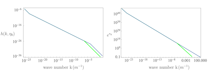
Figure 5: Left panel:Today PGWs strain field $h(k,\eta_{0})$ versus the physical wave number $k^{ph}(m^{-1})$. Right panel: Today PGWs squeezing factor $e^{r_{k}}(\eta_{0})$ versus physical wave number $k_{E}\leq k^{ph}\leq k_{1}$ for $\beta=-2.0$, $\beta_{s}=1$ and $\text{r}=10^{-2}$. The green and blue curves correspond to $T_{reh}=10^{8},10^{10}$ GeV, respectively.

The value of upper frequency of PGWs, $\nu_{1}=ck_{1}/2\pi$, depends on the choice of the increase parameter $\zeta_{1}$. The modes whose frequency is higher than $\nu_{1}$ decay with the expansion of the universe and didn’t get squeezed at all. The value of $\nu_{1}$ should be below the constraint from the rate of the primordial nucleosynthesis (PN) $\nu_{up}\simeq 4\times 10^{10}Hz$ [107, 106], which will in turn exerts constraints on $T_{reh},\beta_{s},\zeta_{1}$, as implied by Eq. (A.1).

Appendix B Gravitational induced-decoherence of the EM field

B.1 Quantum dynamics of the EM field in the presence of PGWs background

Quantum mechanical interaction between GWs and EM field can be encapsulated in the following interaction Hamiltonian [93]

$$\hat{H}_{int}/\hbar = -\frac{1}{2}\frac{\sqrt{16\pi c^{3}}}{(2\pi)^{3/2}}\left(\frac{\hbar\omega_{0}}{E_{Pl}}\right)\sum_{\gamma=+,\times}\int\frac{d^{3}\mathbf{K}}{\sqrt{2\Omega_{K}}}F_{\gamma}(\hat{\mathbf{K}},\hat{\mathbf{k}})\left(\hat{b}_{\mathbf{K},\gamma}e^{-i\Omega_{K}t}+\hat{b}_{\mathbf{K},\gamma}^{\dagger}e^{i\Omega_{K}t}\right)\hat{a}^{\dagger}\hat{a},$$ (B.1)

where $\omega_{0}$ is the EM frequency and $K=(\Omega_{K}/c,\mathbf{K})$ is the GWs four-momentum. The contribution of geometrical configuration of the EM field with respect to the incoming GWs is included in the function $F_{\gamma}(\hat{\mathbf{K}},\hat{\mathbf{k}})=\hat{e}_{ij}^{\gamma}[\hat{\mathbf{K}}]\hat{k}_{i}\hat{k}_{j}$, where $\hat{e}_{ij}^{\gamma}$ stands for the polarization tensor of the GWs with wave vector $\mathbf{K}$, and $\hat{k}$ represents the propagation direction of the EM field. In this expression, $t$ is abbreviation of the delayed time $t_{del}\equiv t-\hat{K}\cdot\mathbf{r}/c=t-\frac{r}{c}\mathbf{K}\cdot\hat{r}=t-\frac{r}{c}\cos\psi_{\hat{r}}$ where $\psi_{\hat{r}}$ is the angle between GWs wave vector and an observation point $\mathbf{r}$ with respect to some frame. Following the quantum Heisenberg equations, it can be shown that the ladder operators of the EM field obey [93]

$$\hat{a}_{\mathbf{k}}(\mathbf{r},t)=e^{-\int d^{3}\mathbf{K}\kappa(\mathbf{K},\mathbf{k})\left(\hat{b}^{\dagger}_{K}\eta_{K}(\mathbf{r},t)-\hat{b}_{K}\eta^{\ast}_{K}(\mathbf{r},t)\right)}e^{iM_{\mathbf{k}}(\mathbf{r},t)\left(1+2\hat{a}^{\dagger}\hat{a}\right)},$$ (B.2)

where $\eta_{K}(\mathbf{r},t)=1-e^{i\Omega_{K}(t-\frac{r}{c}\hat{K}\cdot\hat{r})}$ and

$$\kappa(\mathbf{K},\mathbf{k}) = \frac{1}{4\pi}\left(\frac{\hbar\omega_{0}}{E_{Pl}}\right)K^{-3/2}F_{\gamma}(\hat{\mathbf{K}},\mathbf{k}),$$ (B.3)

could be interpreted as the coupling strength between EM field and quantum GWs and

$$M_{\mathbf{k}}(\mathbf{r},t) = \int d^{3}K\kappa^{2}(\mathbf{K},\mathbf{k})\left(\Omega_{K}(t-\frac{r}{c}\hat{K}\cdot\hat{r})-\sin[\Omega_{K}(t-\frac{r}{c}\hat{K}\cdot\hat{r}]\right).$$ (B.4)

B.2 EM field correlations in the presence of PGWs background

In this section, we investigate the effect of the PGWs background on spatial field correlations of light coming from a distant source. This can be accomplished by considering a Michelson stellar-interferometer setup as depicted in Fig. 6, which was primarily used to measure the angular separation of a binary star or the angular diameter of an extended source. Two EM wave vectors $\mathbf{k}$ and $\mathbf{k}^{\prime}$ illuminate two mirrors $M_{1}$ and $M_{2}$ located at $\mathbf{r}_{1}$ and $\mathbf{r}_{2}$, respectively. By beating the collected light at a point $P$ chosen so that two paths $\overline{M_{1}P}$ and $\overline{M_{2}P}$ are equal, the intensity at point $P$ is measured so as $I\sim I_{0}\{1+\cos[(\mathbf{k}+\mathbf{k})\cdot(\mathbf{r}_{1}-\mathbf{r}_{2})/2]\cos[(\mathbf{k}-\mathbf{k})\cdot(\mathbf{r}_{1}-\mathbf{r}_{2})/2]\}$ [110], where the interference pattern stems from spatial correlations of the source. More generally, spatial correlations are responsible for Young’s double slit interference and Hanbury Brown-Twiss (HB-T) intensity correlations as well, as implied by the van-Citter Zernik theorem [17]. However, existence of PGWs affect spatial correlations as follows; One may consider first order correlation function $\Gamma^{(1)}$ defined by Eq. (3.1) that accounts for the interference patter of the field correlations. We may calculate it for the setup shown in Fig. LABEL:fig:fig6 by specifying the positive frequency-part of the electric field at the location of mirrors as

$$\hat{E}^{(+)}(\mathbf{r}_{i},t_{i})=\mathcal{E}_{k}\left(\hat{a}_{k}(\mathbf{r}_{i},t_{i})e^{i\mathbf{k}\cdot\mathbf{r}_{i}}+\hat{a}_{k^{\prime}}(\mathbf{r}_{i},t_{i})e^{i\mathbf{k}^{\prime}\cdot\mathbf{r}_{i}}\right)$$ (B.5)

where $i=1,2$ and $\hat{a}_{\mathbf{k}}(\mathbf{r}_{i},t_{i})$ is defined in Eq. (B.2). Substituting Eq. B.5 and and its hermitian conjugate into Eq. (3.1) results in

$$\Gamma^{(1)}(\mathbf{r}_{1},t_{1};\mathbf{r}_{2},t_{2}) = \text{Re}[\langle\hat{E}^{(-)}(\mathbf{r}_{1},t_{1})\hat{E}^{(+)}(\mathbf{r}_{2},t_{2})\rangle]$$

$$\sim \text{Re}\left[\langle\hat{a}_{\mathbf{k}}^{\dagger}(\mathbf{r}_{1},t_{1})\hat{a}_{\mathbf{k}}(\mathbf{r}_{2},t_{2})\rangle e^{-i\mathbf{k}\cdot(\mathbf{r}_{1}-\mathbf{r}_{2})}+\mathbf{k}\longleftrightarrow\mathbf{k}^{\prime}\right],$$

where the expectation value is taken over $\hat{\rho}(t)=\hat{\rho}_{\text{pgws}}\otimes\hat{\rho}_{\mathbf{k}}\otimes\hat{\rho}_{\mathbf{k}^{\prime}}$ and each signal is in its own state. It follows

$$\langle\hat{a}_{\mathbf{k}}^{\dagger}(\mathbf{r}_{1},t_{1})\hat{a}_{\mathbf{k}}(\mathbf{r}_{2},t_{2})\rangle = \mathcal{A}_{\mathbf{k}}(\mathbf{r}_{1},t_{1};\mathbf{r}_{2},t_{2})e^{-i(M_{\mathbf{k}}(\mathbf{r}_{1},t_{1})-M_{\mathbf{k}}(\mathbf{r}_{2},t_{2}))}e^{i\omega_{0}(t_{1}-t_{2})}$$

$$\times \Big{\langle}\hat{a}_{\mathbf{k}}^{\dagger}e^{-2iM_{\mathbf{k}}(\mathbf{r}_{1},t_{1})\hat{a}_{\mathbf{k}}^{\dagger}\hat{a}_{\mathbf{k}}}e^{2iM_{\mathbf{k}}(\mathbf{r}_{1},t_{2})\hat{a}_{\mathbf{k}}^{\dagger}\hat{a}_{\mathbf{k}}}\hat{a}_{\mathbf{k}}\Big{\rangle}_{\hat{\rho}_{\mathbf{k}}},$$

where

$$\mathcal{A}_{\mathbf{k}}(\mathbf{r}_{1},t_{1};\mathbf{r}_{2},t_{2})\equiv\bigg{\langle}e^{\int d^{3}\mathbf{K}\kappa(\mathbf{K},\mathbf{k})\left(\hat{b}^{\dagger}_{\mathbf{K}}\eta_{K}(\mathbf{r}_{1},t_{1})-\hat{b}_{\mathbf{K}}\eta^{\ast}_{K}(\mathbf{r}_{1},t_{1})\right)}e^{-\int d^{3}\mathbf{K}\kappa(\mathbf{K},\mathbf{k})\left(\hat{b}^{\dagger}_{\mathbf{K}}\eta_{K}(\mathbf{r}_{2},t_{2})-\hat{b}_{\mathbf{K}}\eta^{\ast}_{K}(\mathbf{r}_{2},t_{2})\right)}\bigg{\rangle}_{\hat{\rho}_{\text{pgws}}}.$$ (B.8)

Since $M_{\mathbf{k}}(\mathbf{r}_{1},t)\propto\kappa^{2}(\mathbf{K},\mathbf{k})\propto\left(\hbar\omega_{0}/E_{Pl}\right)^{2}$ is negligibly small, one may disregard terms containing $M_{\mathbf{k}}(\mathbf{r}_{i},t_{i})$ in expression Eq. (B.2), that basically causes coherent phase modulation. On the other hand, here we consider PGWs quantum state to be the multi-mode squeezed state, $\hat{\rho}_{\text{pgws}}=\prod_{K}\hat{\mathcal{S}}^{\dagger}(\zeta_{K})|0_{K}\rangle\langle 0_{K}|\hat{\mathcal{S}}(\zeta_{K})$ with $\hat{\mathcal{S}}$ being the squeezing operator, $\zeta_{K}\equiv r_{K}e^{i\theta_{\zeta_{K}}}$ being the squeezing parameter and $(r_{K},\theta_{\zeta_{K}})$ being the squeezing amplitude and angle, respectively. The squeezing amplitude $r_{K}$ is determined by Eq. (2.2). The squeezing angle $\theta_{\zeta_{K}}$ for super-horizon modes tends to either $0$ or $\pi$, while for sub-horizon modes leads to harmonically oscillating phase [20], that is already contributed in the Hamiltonian Eq. (B.1). Since due to causality we consider the interaction between EM and sub-horizon PGWs modes (see Sec. C.2 for details), we may proceed by taking $\theta_{\zeta_{K}}=0$. One ends up with

$$\Gamma^{(1)}(\mathbf{r}_{1},t_{2};\mathbf{r}_{2},t_{2}) = \text{Re}\left[\mathcal{A}_{\mathbf{k}}^{\text{sq}}(\mathbf{r}_{1},t_{1};\mathbf{r}_{2},t_{2})\langle\hat{a}_{\mathbf{k}}^{\dagger}\hat{a}_{\mathbf{k}}\rangle e^{-i\mathbf{k}\cdot(\mathbf{r}_{1}-\mathbf{r}_{2})+i\omega_{0}(t_{1}-t_{2})}+\mathbf{k}\longleftrightarrow\mathbf{k}^{\prime}\right],$$ (B.9)

where the decaying amplitude for the squeezed PGWs turns out

$$\mathcal{A}_{\mathbf{k}}^{\text{sq}}(\mathbf{r}_{1},t_{1};\mathbf{r}_{2},t_{2}) = \mathcal{A}_{\mathbf{k}}^{\text{vac}}(\mathbf{r}_{1},t_{1};\mathbf{r}_{2},t_{2})e^{-\mathcal{B}_{\mathbf{k}}^{\text{sq}}(\mathbf{r}_{1},t_{1};\mathbf{r}_{2},t_{2})},$$ (B.10)

The contribution of vacuum is define by Eq. (4.1), and the function $\mathcal{B}_{\mathbf{k}}^{\text{sq}}(\mathbf{r}_{1},t_{1};\mathbf{r}_{2},t_{2})$ is defined by

$$\mathcal{B}_{\mathbf{k}}^{\text{sq}}(\mathbf{r}_{1},t_{1};\mathbf{r}_{2},t_{2}) = \int d^{3}\mathbf{K}\kappa^{2}(\mathbf{K},\mathbf{k})\bigg{\{}\sinh^{2}(r_{K})\Big{(}4\sin^{2}\big{[}\frac{\Omega_{K}(t_{1}-t_{2})}{2}\big{]}\Big{)}$$

$$+ \frac{1}{2}\sinh(2r_{K})\Big{(}\cos\left[2\Omega_{K}t_{1}\right]+\cos\left[2\Omega_{K}t_{2}\right]-2\cos\left[\Omega_{K}(t_{1}+t_{2})\right]\Big{)}\bigg{\}}.$$

where the contributions of mean number of gravitons and correlation between them are represented by the first and second terms on the r.h.s of Eq. (B.2), respectively. Here, $t_{1}$ and $t_{2}$ are abbreviations of the delayed time (see Sec. B.1). To proceed, we shall assume that the mean number of photons in each mode $\mathbf{k}$ and $\mathbf{k}^{\prime}$ is the same, and consider the normalized correlation function $\gamma^{(1)}(\mathbf{r}_{1},t_{1},\mathbf{r}_{2},t_{2})\equiv\frac{\Gamma^{(1)}(\mathbf{r}_{1},t_{1},\mathbf{r}_{2},t_{2})}{\langle\hat{a}^{\dagger}\hat{a}\rangle}$. Moreover, we shall show that the decaying amplitude $\mathcal{A}_{\mathbf{k}}^{\text{sq}}(\mathbf{r}_{1},t_{1};\mathbf{r}_{2},t_{2})$ is the same for both modes $\mathbf{k}$ and $\mathbf{k}^{\prime}$, so that Eq. (B.8) results in

$$\gamma^{(1)}(\mathbf{r}_{1},t_{2};\mathbf{r}_{2},t_{2}) = \mathcal{A}_{\mathbf{k}}^{\text{sq}}(\mathbf{r}_{1},t_{1};\mathbf{r}_{2},t_{2})\cos\left(\frac{(\mathbf{k}+\mathbf{k}^{\prime})\cdot(\mathbf{r}_{1}-\mathbf{r}_{2})}{2}\right)\cos\left(\frac{(\mathbf{k}-\mathbf{k}^{\prime})\cdot(\mathbf{r}_{1}-\mathbf{r}_{2})}{2}\right),$$ (B.12)

This expression describes the interference pattern appearing in a typical Michelson stellar interferometer, stemming from spatial coherence of radiation [17]. However, PGWs background introduce a decaying prefactor which may spoil the interference pattern. More generally, it can be shown that higher order correlation functions of the field, such as intensity correlations, also suffer from the same decaying behaviour of the correlations. Hence, to ruin the phase correlations of the EM field is a characteristic feature of the PGWs background which induces phase incoherence that lead spatial correlations of the field to vanish. In next sections, we investigate $\mathcal{A}_{\mathbf{k}}^{\text{sq}}(\mathbf{r}_{1},t_{1};\mathbf{r}_{2},t_{2})$ and look for circumstances that PGWs don’t spoil spatial correlations.

B.3 Spatial incoherence induced by PGWs

B.3.1 Configuration of the ineterferometer

In order to perform integrals involved in Eq. (B.10), we consider a typical Michelson stellar interferometer configuration depicted in Fig. 6(a): the origin of coordinate system is chosen at the center of the (quasi) planar source with radius $a$; two detectors located at $P_{1}$ and $P_{2}$ lay along $x-$axis with a separation $d_{12}=|\mathbf{r}_{1}-\mathbf{r}_{2}|$ perpendicular to $z-$ axis; GWs propagation direction makes angle $\Theta_{K}$ with $z-$axis; Two EM signals with wave vectors $\mathbf{k}$ and $\mathbf{k}^{\prime}$ from two distant edges of the source incidence both detectors, making angles $\theta_{\mathbf{k}}=\theta/2$ and $\theta_{\mathbf{k}^{\prime}}=-\theta/2$ with $z-$axis respectively, where $\theta\equiv 2a/|\mathbf{r}|$ is the angular diameter subtended by the source when viewed from $P_{1}P_{2}$.

Before proceed, one may note that the function $F_{\gamma}(\hat{\mathbf{K}},\hat{\mathbf{k}})=\hat{e}_{ij}[\hat{\mathbf{K}}]\hat{k}_{i}\hat{k}_{j}$ that describes EM-GWs coupling is an invariant quantity that doesn’t depend on the choice of the coordinate system. As a result, one is free to consider a configuration in which $\hat{\mathbf{K}}$ and $\hat{\mathbf{k}}$ are such as shown in Fig. 6. Here, positioning of detectors with respect to line of sight is symmetric, and is a specific case of a more general situation in which the baseline of the interferometer makes an angle $\theta_{s}$ with the line of sight, as is shown in panel (b) of Fig. 6. This can be justified by noticing the fact that, according to the van Citter-Zernik theorem, the light produced by spatially incoherent, quasi-monochromatic, uniform, circular source of radius $a$ is approximately coherent in the far zone and close to the direction normal to the source plane and parallel to it. In practical situation of a typical VLBI instrument, orientation of the source with respect to detectors baseline causes a geometrical delay $\tau_{g}=(\mathbf{r}_{1}-\mathbf{r}_{2})\cdot\mathbf{k}/c$ that is often compensated to achieve equal-time correlations [111]. Panel (c) illustrates the symmetrical configuration where $\theta_{s}=0$. A plane source of radius $a$ is located at the origin of coordinates, illuminating the mirrors $M_{1}$ and $M_{2}$ located at $\mathbf{r}_{1}$ and $\mathbf{r}_{2}$, respectively. The EM wave vectors make angle $\theta$ and $(\Theta_{K},\Phi_{K})$ show spatial angles of the GWs wave vector $\mathbf{K}$.

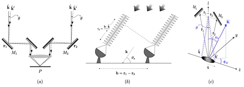
Figure 6: Configuration of the system. Panel (a): a typical Michelson interferometer working based on spatial coherence. Panel (b): a two-detector VLBI apparatus with an asymmetric positioning with respect to the line of sight of the source. Panel (c): Detailed illustration of the physical parameters $\mathbf{r}_{1},\mathbf{r}_{2},\mathbf{k}_{1},\mathbf{k}_{2},\mathbf{K},\theta,\Theta_{K},\Phi_{K}.$

According to Fig. 6(c) one has

$$\hat{\mathbf{k}} = (\sin\theta/2,0,\cos\theta/2),$$

$$\hat{\mathbf{k}}^{\prime} = (-\sin\theta/2,0,\cos\theta/2),$$ (B.13)

$$\hat{\mathbf{K}} = (\sin\Theta_{K}\cos\Phi_{K},\sin\Theta_{K}\sin\Phi_{K},\cos\Theta_{K}).$$

For each mode $\mathbf{k}$ and $\mathbf{k}^{\prime}$ the function $F_{\gamma}(\hat{\mathbf{K}},\hat{\mathbf{k}})$ become

$$F_{\gamma}(\hat{\mathbf{K}},\hat{\mathbf{k}}) = e_{11}^{\gamma}\sin^{2}\theta/2+e_{33}^{\gamma}\cos^{2}\theta/2+e_{13}^{\gamma}\sin\theta\simeq e_{33}^{\gamma}+\theta e_{13}^{\gamma}+\theta^{2}\left(\frac{e_{11}^{\gamma}-e_{33}^{\gamma}}{4}\right),$$

$$F_{\gamma}(\hat{\mathbf{K}},\hat{\mathbf{k}}^{\prime}) = e_{11}^{\gamma}\sin^{2}\theta/2+e_{33}^{\gamma}\cos^{2}\theta/2-e_{13}^{\gamma}\sin\theta\simeq e_{33}^{\gamma}-\theta e_{13}^{\gamma}+\theta^{2}\left(\frac{e_{11}^{\gamma}-e_{33}^{\gamma}}{4}\right).$$ (B.14)

Typical angular sizes of distant objects is of order $\mathcal{O}(\theta)\sim 10^{-8}$ [89] so we may keep terms proportional to $\mathcal{O}(\theta)$ in our calculations,

$$F^{2}_{\gamma}(\hat{\mathbf{K}},\hat{\mathbf{k}}) = [e_{33}^{\gamma}]^{2}+2\theta[e_{13}^{\gamma}][e_{33}^{\gamma}]+\theta^{2}\left([e_{13}^{\gamma}]^{2}+e_{33}^{\gamma}\frac{e_{11}^{\gamma}-e_{33}^{\gamma}}{2}\right),$$

$$F^{2}_{\gamma}(\hat{\mathbf{K}},\hat{\mathbf{k}}^{\prime}) = [e_{33}^{\gamma}]^{2}-2\theta[e_{13}^{\gamma}]^{2}[e_{33}^{\gamma}]+\theta^{2}\left([e_{13}^{\gamma}]^{2}+e_{33}^{\gamma}\frac{e_{11}^{\gamma}-e_{33}^{\gamma}}{2}\right).$$ (B.15)

Hence the coupling function for modes $\mathbf{k}$ and $\mathbf{k}^{\prime}$ differs by a term proportional to $[e_{13}^{\gamma}][e_{33}^{\gamma}]$. According to definition of $\hat{e}_{ij}$ one has

$$\begin{cases}e_{33}^{+}=\sin^{2}\Theta_{K},\\ e_{33}^{\times}=0\end{cases}\quad,\quad\begin{cases}e_{13}^{+}=-\sin\Theta_{K}\cos\Theta_{K}\cos\Phi_{K},\\ e_{13}^{\times}=\sin\Theta_{K}\sin\Phi_{K}.\end{cases}$$ (B.16)

Integration over the azimuthal angle $\Phi_{K}$ yields $\int d\Phi_{K}[e_{13}^{+}][e_{33}^{+}]=0=\int d\Phi_{K}[e_{13}^{\times}][e_{33}^{\times}]$ hence the coupling strength $\kappa(\hat{\mathbf{K}},\hat{\mathbf{k}})$ is the same for $\mathbf{k}$ and $\mathbf{k}^{\prime}$ as one expects intuitively. In fact, physical quantities must be invariant under the replacement $\mathbf{k}\Longleftrightarrow\mathbf{k}^{\prime}$, as it does for the coupling strength $\kappa$ as well as the decaying amplitude $\mathcal{A}$ define by Eqs. (B.9 , B.10). We proceed by defining

$$F^{2}_{\gamma}(\hat{\mathbf{K}},\hat{\mathbf{k}}) \equiv F^{2}_{\gamma}(\hat{\mathbf{K}},\hat{\mathbf{k}}^{\prime})=[e_{33}^{\gamma}]^{2}+\theta^{2}[e_{13}^{\gamma}]^{2}.$$ (B.17)

B.3.2 PGWs induced incoherence length $\xi_{gr}$

The integral over $d^{3}\mathbf{K}$ in Eq. (B.10) can be performed as follows. First note that the times $t_{1}$ and $t_{2}$ are replaced by delay times according to

$$\begin{cases}t_{1}\rightarrow t_{1}-\hat{\mathbf{K}}\cdot\frac{\mathbf{r_{1}}}{c}=t_{1}-\frac{r_{1}}{c}\hat{\mathbf{K}}\cdot\hat{\mathbf{r}}_{1}=t_{1}-\frac{r_{1}}{c}\cos(\Theta_{K}+\frac{d_{12}}{2D}),\\ t_{2}\rightarrow t_{2}-\hat{\mathbf{K}}\cdot\frac{\mathbf{r_{2}}}{c}=t_{2}-\frac{r_{2}}{c}\hat{\mathbf{K}}\cdot\hat{\mathbf{r}}_{2}=t_{2}-\frac{r_{2}}{c}\cos(\Theta_{K}-\frac{d_{12}}{2D})\\ \end{cases}$$ (B.18)

where $|\mathbf{r}_{1}|\simeq|\mathbf{r}_{2}|\simeq|\mathbf{r}|\equiv D$. To first order in $d$ one has

$$\begin{cases}t_{1}\rightarrow t_{1}-\frac{D}{c}\cos\Theta_{K}+\frac{D}{c}\frac{d_{12}}{2D}\sin\Theta_{K},\\ t_{2}\rightarrow t_{2}-\frac{D}{c}\cos\Theta_{K}-\frac{D}{c}\frac{d_{12}}{2D}\sin\Theta_{K},\end{cases}$$ (B.19)

Plugging $\kappa$ from Eq. (B.3) into Eq. (B.2) and replacing $t_{1}$ and $t_{2}$ from Eq. (B.19) yields

$$\mathcal{B}_{\mathbf{k}}^{\text{sq}}(\mathbf{r}_{1},t_{1};\mathbf{r}_{2},t_{2}) = \frac{1}{(4\pi)^{2}}\left(\frac{\hbar\omega_{0}}{E_{Pl}}\right)^{2}\int d\Phi_{K}\int d(\cos\Theta_{K})F^{2}_{\gamma}(\hat{\mathbf{K}},\hat{\mathbf{k}})\int\frac{dK}{K}$$

$$\times \bigg{\{}\sinh^{2}(r_{K})\Big{(}4\sin^{2}\left[\frac{\Omega_{K}}{2}(t_{1}-t_{2}+\frac{d_{12}}{c}\sin\Theta_{K})\right]\Big{)}$$

$$+ \frac{1}{2}\sinh(2r_{K})\Big{(}\cos\left[2\Omega_{K}(t_{1}-\frac{D}{c}\cos\Theta_{K}+\frac{d_{12}}{2c}\sin\Theta_{K})\right]$$

$$+ \cos\left[2\Omega_{K}(t_{2}-\frac{D}{c}\cos\Theta_{K}-\frac{d_{12}}{2c}\sin\Theta_{K})\right]-2\cos\left[\Omega_{K}(t_{1}+t_{2}-\frac{2D}{c}\cos\Theta_{K})\right]\Big{)}\bigg{\}}.$$

where $F_{\gamma}(\hat{\mathbf{K}},\hat{\mathbf{k}})$ is given by Eq. (B.16). Here, $t_{1}$ and $t_{2}$ are the propagation time intervals of the EM field through the PGWs background, hence one may write $t_{1}\simeq t_{2}\simeq\frac{D}{c}\equiv t_{int}$, so that the equal-time EM correlations after a long time of interaction with PGWs background is obtained. Expanding terms in powers of $d_{12}$ and keep terms up to $\mathcal{O}(d_{12}^{2})$ results in

$$\Big{(}Kd_{12}\sin\Theta_{K}\Big{)}^{2}\bigg{\{}\bar{n}_{\text{sq}}(K)-\frac{1}{2}\sinh(2r_{k})\cos\Big{[}2\Omega_{K}t_{\text{int}}(1-\cos\Theta_{K})\Big{]}\bigg{\}}$$ (B.21)

and Eq. (B.3.2) becomes

$$\mathcal{B}^{\text{sq}}_{\mathbf{k}}(\mathbf{r}_{1},t_{1};\mathbf{r}_{2},t_{2}) = \bigg{(}\frac{1}{(4\pi)^{2}}\left(\frac{\hbar\omega_{0}}{E_{Pl}}\right)^{2}\int d\Phi_{K}\int d(\cos\Theta_{K})F^{2}_{\gamma}(\hat{\mathbf{K}},\hat{\mathbf{k}})\sin^{2}\Theta_{K}$$

$$\times \int KdK\Big{\{}\bar{n}_{\text{sq}}(K)-\frac{1}{2}\sinh(2r_{k})\cos\Big{[}2\Omega_{K}t_{\text{int}}(1-\cos\Theta_{K})\Big{]}\Big{\}}\bigg{)}d_{12}^{2}.$$

$$\equiv \xi_{\text{sq}}^{-2}d_{12}^{2}$$

In last line of Eq. (B.3.2), we have defined the incoherence length induced by squeezed PGWs, $\xi_{\text{sq}}$, as

$$\xi_{\text{sq}} \equiv \bigg{[}\frac{1}{(4\pi)^{2}}\left(\frac{\hbar\omega_{0}}{E_{Pl}}\right)^{2}\int d\Phi_{K}\int d(\cos\Theta_{K})F^{2}_{\gamma}(\hat{\mathbf{K}},\hat{\mathbf{k}})\sin^{2}\Theta_{K}$$

$$\times \int KdK\Big{(}\bar{n}_{\text{sq}}(K)-\frac{1}{2}\sinh(2r_{k})\cos\Big{[}2\Omega_{K}t_{\text{int}}(1-\cos\Theta_{K})\Big{]}\Big{)}\bigg{]}^{-1/2},$$

and the decaying amplitude Eq. (B.10) becomes

$$\mathcal{A}(\mathbf{r}_{1},t_{1};\mathbf{r}_{2},t_{2})=e^{-\left(\frac{d_{12}}{\xi_{\text{sq}}}\right)^{2}},$$ (B.24)

The final expression of the two-point correlation function Eq. (B.9) outcomes

$$\gamma^{(1)}(\mathbf{r}_{1},t_{1};\mathbf{r}_{2},t_{2}) = e^{-\left(\frac{d_{12}}{\xi_{\text{sq}}}\right)^{2}}\cos\left(\frac{(\mathbf{k}+\mathbf{k}^{\prime})\cdot(\mathbf{r}_{1}-\mathbf{r}_{2})}{2}\right)\cos\left(\frac{(\mathbf{k}-\mathbf{k}^{\prime})\cdot(\mathbf{r}_{1}-\mathbf{r}_{2})}{2}\right)$$ (B.25)

$$= e^{-\left(\frac{d_{12}}{\xi_{\text{sq}}}\right)^{2}}\cos\left(kd_{12}\theta/2\right),$$

where in last line of we replaced $(\mathbf{k}+\mathbf{k}^{\prime})\cdot(\mathbf{r}_{1}-\mathbf{r}_{2})=0$ and $(\mathbf{k}-\mathbf{k}^{\prime})\cdot(\mathbf{r}_{1}-\mathbf{r}_{2})=kd_{12}\theta$ according to the aforementioned configuration. Eq. (B.24) implies that as a consequence of interaction with PGWs, the interference pattern disappears provided that $d_{12}\gtrsim\xi_{\text{sq}}$. The induced incoherence length $\xi_{\text{sq}}$ inversely depends on the squeezing factor $e^{2r}$ as well as on the initial amplitude of tensor perturbations through Eq. (2.2). Higher squeezing of PGWs or larger initial amplitude of tensor perturbations shrink the correlation length $\xi_{\text{sq}}$ more, so as leading to a more strength decaying amplitude.

It is easier to work with the dimensionless coherence parameter $\alpha_{\text{sq}}\equiv\log(k_{0}d_{12})$ where $k_{0}=\omega_{0}/c$ being the EM wave number. Eq. (B.3.2) results in

$$\alpha_{\text{sq}}(\beta,\beta_{s},T_{reh},\text{r}) = \bigg{[}\frac{1}{(4\pi)^{2}}\left(\frac{\hbar c}{E_{Pl}}\right)^{2}\int d\Phi_{K}\int d(\cos\Theta_{K})F^{2}_{\gamma}(\hat{\mathbf{K}},\hat{\mathbf{k}})\sin^{2}\Theta_{K}$$

$$\times \int KdK\Big{(}\bar{n}_{\text{sq}}(K)-\frac{1}{2}\sinh(2r_{k})\cos\Big{[}2\Omega_{K}t_{\text{int}}(1-\cos\Theta_{K})\Big{]}\Big{)}\bigg{]}^{-1/2},$$

where $F^{2}_{\gamma}(\hat{\mathbf{K}},\hat{\mathbf{k}})$ is given by Eq. (B.17), $(\beta,\beta_{s},T_{reh},\text{r})$-dependence of $e^{r_{K}}$ is determined by Eq. (2.2) and the integration limit is $k_{E}\leq k\leq k_{1}$.

The light detected today was emitted at some earlier time $t_{em}$. The interaction time $t_{int}$ appearing in Eq. (B.3.2) is the time of flight of the EM field from emission time $t_{em}$ to detection time at present $t_{0}$. In next section, we incorporate the cosmological expansion of the FLRW background meantime the EM field propagates from the source to the Earth.

Appendix C Incorporating cosmological expansion

C.1 Expression of $t_{\text{int}}$ in terms of the redshift $z$

In order to prob the incoherence induced by PGWs, we consider a set of intermediate-luminosity radio quasars whose angular size-redshift are accurately measure by VLBI means, i.e., based on spatial coherence of the emitted EM radiation (see Fig. 7). These objects are located at redshift range $0.46\leq z\leq 2.73$, so during their journey to the Earth, they have been affected not only by PGWs background, but also by the expansion of the Universe. One may incorporate the Universe expansion by expressing time, distance and frequency in terms of redshift. In particular, one may replace the EM frequency $\omega_{0}\rightarrow\omega_{0}/(1+z_{\ast})$ where $z_{\ast}$ stands for the redshift of the source. The light detected today was emitted at some earlier time. The interaction time $t_{int}$ that is the time interval between emission at time $t_{z_{\ast}}$ and detection at a later time $t_{z}$, can be related to redshift $z$ according to [114]

$$t_{int}=t_{z}-t_{z_{\ast}}\equiv t(z,z_{\ast})=\int_{z}^{z_{\ast}}\frac{dz^{\prime}}{(1+z^{\prime})H(z^{\prime})},$$ (C.1)

where $H(z)$ is the Hubble parameter. For a flat Universe comprising only cold dark matter and a cosmological constant, so that $\Omega_{0}=\Omega_{\Lambda}+\Omega_{m}=1$, one has

$$H(z)=H_{0}\sqrt{(1-\Omega_{m})+\Omega_{m}(1+z)^{3}}.$$ (C.2)

and the interaction time Eq. (C.1) outcomes

$$t_{int}(z,z_{\ast})=H_{0}^{-1}\int_{z}^{z_{\ast}}\frac{dz^{\prime}}{\sqrt{(1-\Omega_{m})(1+z^{\prime})^{2}+\Omega_{m}(1+z^{\prime})^{5}}},$$ (C.3)

C.2 Particle horizon and delayed interaction of EM field with PGWs inside the horizon

At the moment of EM emission from a source located at $z_{\ast}$, say $\eta_{\ast}$, the EM field can only interact with PGWs modes that are already reentered the horizon, since it doesn’t have causal contact with modes with wave lengths larger than the Hubble radius at that moment, i.e, with modes with $\lambda_{k}\geq 1/\mathcal{H}$. As time passes, new modes reenter the horizon and the EM field can interact with them at a later time $\eta$. We may call this later interaction as delayed interaction. The situation is schematically described in Fig. 7: vertical axis shows the Hubble radius $\mathcal{H}(\eta)$ (multiplied by $2\pi$ factor) versus comoving time $\eta$. A typical EM source located at $z_{\ast}$ emits light at $\eta_{\ast}$ which will be detected at time $\eta_{0}$. The EM field interacts only with a PGWs mode which are inside the horizon, i.e., with $k\geq k(\eta_{\ast})$. Gradually, new modes reenter the horizon and there would be interaction with those modes at later times. As a result, the interaction time $t_{int}$ generally depends on PGWs mode $k$.

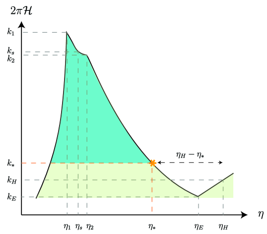
Figure 7: Schematic view of Hubble radius $2\pi\mathcal{H}(\eta)$ versus comoving time $\eta$ corresponding to the expanding Universe Eq. (2.1). A typical PGWs mode $k$ leaves the horizon during inflation and re-enter it at subsequent epochs. The colored regions show the time interval during which the mode $k$ is outside the horizon. For a source located at $z_{\ast}$, the interaction time $\eta_{H}-\eta_{\ast}$ not only depends on $z_{\ast}$ but also depends on the particle horizon at the moment of emission $\eta_{\ast}$: modes with $k\geq k_{\ast}$ reside the horizon (shown by blue region) while $k\leq k_{\ast}$ reenter the horizon at later times (shown by green region).

In order to find $k-$dependence of the interaction time $t_{int}$, we first consider three sub-regions $0\leq z_{\ast}\leq z_{E}$, $z_{E}\leq z_{\ast}\leq z_{H}$ and $z_{\ast}\geq z_{H}$. For each case, the PGWs modes inside the horizon and the corresponding interaction time differs. We consider each case separately.

C.2.1 $z_{\ast}\geq z_{H}$

During the matter-dominated era, the characteristic wave number is related to the redshift $z$ according to

$$1+z(k)=\frac{a(\eta_{0})}{a(\eta_{k}}=\frac{a(\eta_{0})}{a(\eta_{E})}\frac{a(\eta_{E})}{a(\eta_{k})}=\zeta_{E}\left(\frac{k}{k_{E}}\right)^{2}\quad\rightarrow\quad k=k_{E}\sqrt{(1+z_{k})\zeta_{E}^{-1}}.$$ (C.4)

For objects with $z_{\ast}\geq z_{E}=0.33$ the emission time $\eta_{\ast}$ resides in the matter-dominated are. In this case, Eq. (C.4) gives the characteristic wave number at emission time $\eta_{\ast}$ is given by $k_{\ast}=k_{E}\sqrt{(1+z_{\ast})\zeta_{E}^{-1}}$. Moreover, at the time $\eta_{H_{1}}$ which $k_{H}$ leaves the horizon during matter-dominated era, one has $1+z_{H}=\zeta_{E}^{3}\simeq 2.35$ or $z_{H}\simeq 1.35$.

• Modes with $k\geq k_{\ast}$ always stay inside the horizon and the interaction time $t_{int}=t_{0}-t_{z_{\ast}}=t(0,z_{\ast})$ is given by

  $$t_{int}=H_{0}^{-1}\int_{0}^{z_{\ast}}\frac{dz^{\prime}}{\sqrt{(1-\Omega_{m})(1+z^{\prime})^{2}+\Omega_{m}(1+z^{\prime})^{5}}}\quad,\quad k\geq k_{\ast}$$ (C.5)

• Modes with $k_{H}\leq k\leq k_{\ast}$ reenter the horizon at a later time $\eta_{z}$ and stay inside the horizon by $\eta_{0}$, hence the interaction time $t_{int}(k)=t_{0}-t_{z(k)}$ is given by

  $$t_{int}(k)=H_{0}^{-1}\int_{0}^{z(k)}\frac{dz^{\prime}}{\sqrt{(1-\Omega_{m})(1+z^{\prime})^{2}+\Omega_{m}(1+z^{\prime})^{5}}}\quad,\quad k_{H}\leq k\leq k_{\ast}$$ (C.6)

  where $z(k)$ obeys Eq. (C.4) that is $z(k)=\zeta_{E}(k/k_{E})^{2}-1$ and $z_{H}\geq z(k)\geq z_{\ast}$.

• Modes with $k_{E}\leq k\leq k_{H}$ reenter the horizon at a time $\eta_{z}$ during matter-dominated era and again leave the horizon at $\eta_{z_{\ast\ast}}$ during $\Lambda$-dominated era, where $0\leq z_{\ast\ast}\leq z_{E}$. The interaction time $t_{int}(k)=t_{z_{\ast\ast}}(k)-t_{z}(k)$ is given by

  $$t_{int}(k)=H_{0}^{-1}\int_{z_{\ast\ast}(k)}^{z(k)}\frac{dz^{\prime}}{\sqrt{(1-\Omega_{m})(1+z^{\prime})^{2}+\Omega_{m}(1+z^{\prime})^{5}}}\quad,\quad k_{E}\leq k\leq k_{H}$$ (C.7)

  where $z_{\ast\ast}(k)$ obeys

  $$1+z_{\ast\ast}(k)=\frac{a(\eta_{0})}{a(\eta_{z_{\ast\ast}})}=\left(\frac{k_{H}}{k}\right).$$ (C.8)

C.2.2 $z_{E}\leq z_{\ast}\leq z_{H}$

For objects with $z_{E}\leq z_{\ast}\leq z_{H}$ the corresponding characteristic wave number $k_{\ast}$ is determined by Eq. (C.9).

• PGWs modes with $k\geq k_{H}$ always stay inside the horizon and the interaction time $t_{int}=t_{0}-t_{z_{\ast}}=t(0,z_{\ast})$ is given by Eq.(C.5).

• Modes with $k_{\ast}\leq k\leq k_{H}$ have been inside the horizon from emission time $\eta_{\ast}$ and leave the horizon at a later time $\eta_{z_{\ast\ast}}$ during $\Lambda-$dominated era. The interaction time $t_{int}(k)=t_{z_{\ast\ast}}(k)-t_{z_{\ast}}$ is given by

  $$t_{int}(k)=H_{0}^{-1}\int_{z_{\ast\ast}(k)}^{z_{\ast}}\frac{dz^{\prime}}{\sqrt{(1-\Omega_{m})(1+z^{\prime})^{2}+\Omega_{m}(1+z^{\prime})^{5}}}\quad,\quad k_{\ast}\leq k\leq k_{H}$$ (C.9)

  where $z_{\ast\ast}(k)$ is determined by Eq. (C.8)

• Modes with $k_{E}\leq k\leq k_{\ast\ast}$ reenter the horizon at a time $\eta_{z}$ during matter-dominated era and leave it at a time $\eta_{z_{\ast\ast}}$ during $\Lambda-$dominated era. The interaction time $t_{int}(k)=t_{z_{\ast\ast}(k)}-t_{z(k)}$ is given by Eq. (C.7) where $z(k)$ and $z_{\ast\ast}(k)$ are given by Eqs. (C.4,C.8), respectively.

C.2.3 $z_{\ast}\leq z_{E}$

For objects with $z_{\ast}\leq z_{E}$ the corresponding characteristic wave number $k_{\ast}$ can be determined by Eq. (C.8).

• PGWs modes with $k\geq k_{H}$ always stay inside the horizon and the interaction time $t_{int}=t_{0}-t_{z_{\ast}}=t(0,z_{\ast})$ is given by Eq.(C.5).

• Modes with $k_{\ast}\leq k\leq k_{H}$ have been inside the horizon from emission time $\eta_{\ast}$ and leave the horizon at a later time $\eta_{z_{\ast\ast}}$ during $\Lambda-$dominated era. The interaction time $t_{int}(k)=t_{z_{\ast\ast}}(k)-t_{z_{\ast}}$ is given by

  $$t_{int}(k)=H_{0}^{-1}\int_{z_{\ast\ast}(k)}^{z_{\ast}}\frac{dz^{\prime}}{\sqrt{(1-\Omega_{m})(1+z^{\prime})^{2}+\Omega_{m}(1+z^{\prime})^{5}}}\quad,\quad k_{\ast}\leq k\leq k_{H}$$ (C.10)

  where $z_{\ast\ast}(k)$ is determined by Eq. (C.8)

• Modes with $k_{E}\leq k\leq k_{\ast\ast}$ reenter the horizon at a time $\eta_{z}$ during matter-dominated era and leave it at a time $\eta_{z_{\ast\ast}}$ during $\Lambda-$dominated ear. The interaction time $t_{int}(k)=t_{z_{\ast\ast}(k)}-t_{z_{\ast}}$ is given by Eq. (C.9) where $z_{\ast\ast}$ is given by Eq. (C.8).

• Modes with $k\leq k_{\ast}$ always reside out of the horizon.

By substituting the interaction time $t_{int}(k)$ from previous expressions into Eq. (B.25) and performing integration with respect to PGWs modes $(K,\Theta_{K},\Phi_{K})$, the curves $\alpha_{gr}-z$ can be obtained, for given values of ($\beta,\beta_{s},T_{reh},\text{r}$).

References

- Saulson [1994] P. R. Saulson, Fundamentals of interferometric gravitational wave detectors (World Scientific, 1994).
- Barish and Weiss [1999] B. C. Barish and R. Weiss, Ligo and the detection of gravitational waves, Physics Today 52, 44 (1999).
- Ju et al. [2000] L. Ju, D. Blair, and C. Zhao, Detection of gravitational waves, Reports on Progress in Physics 63, 1317 (2000).
- Accadia et al. [2012] T. Accadia, F. Acernese, M. Alshourbagy, P. Amico, F. Antonucci, S. Aoudia, N. Arnaud, C. Arnault, K. Arun, P. Astone, et al., Virgo: a laser interferometer to detect gravitational waves, Journal of Instrumentation 7 (03), P03012.
- Blair et al. [2012] D. G. Blair, E. J. Howell, L. Ju, and C. Zhao, Advanced gravitational wave detectors (Cambridge University Press, 2012).
- Garay [1998] L. J. Garay, Spacetime foam as a quantum thermal bath, Physical Review Letters 80, 2508 (1998).
- Kempf [1999] A. Kempf, On the three short-distance structures which can be described by linear operators, Reports on Mathematical Physics 43, 171 (1999).
- Rovelli [2008] C. Rovelli, Loop quantum gravity, Living reviews in relativity 11, 1 (2008).
- Amelino-Camelia [2000] G. Amelino-Camelia, Gravity-wave interferometers as probes of a low-energy effective quantum gravity, Physical Review D 62, 024015 (2000).
- Lieu and Hillman [2003] R. Lieu and L. W. Hillman, The phase coherence of light from extragalactic sources: Direct evidence against first-order planck-scale fluctuations in time and space, The Astrophysical Journal 585, L77 (2003).
- Ragazzoni et al. [2003] R. Ragazzoni, M. Turatto, and W. Gaessler, The lack of observational evidence for the quantum structure of spacetime at planck scales, The Astrophysical Journal 587, L1 (2003).
- Lämmerzahl [2005] C. Lämmerzahl, Interferometry as a universal tool in physics, in Planck Scale Effects in Astrophysics and Cosmology (Springer, 2005) pp. 161–198.
- Lämmerzahl [2007] C. Lämmerzahl, The search for quantum gravity effects, Quantum Gravity: Mathematical Models and Experimental Bounds , 15 (2007).
- Khodadi et al. [2019] M. Khodadi, K. Nozari, A. Bhat, and S. Mohsenian, Probing planck-scale spacetime by cavity opto-atomic rb interferometry, Progress of Theoretical and Experimental Physics 2019, 053E03 (2019).
- Ng et al. [2003] Y. J. Ng, W. A. Christiansen, and H. van Dam, Probing planck-scale physics with extragalactic sources?, The Astrophysical Journal 591, L87 (2003).
- Coule [2003] D. Coule, Planck scale still safe from stellar images, Classical and Quantum Gravity 20, 3107 (2003).
- Mandel and Wolf [1995] L. Mandel and E. Wolf, Optical coherence and quantum optics (Cambridge university press, 1995).
- Grishchuk [1977] L. Grishchuk, Graviton creation in the early universe, Annals of the New York Academy of Sciences 302, 439 (1977).
- Grishchuk [1997] L. Grishchuk, The implications of microwave background anisotropies for laser-interferometer-tested gravitational waves, Classical and Quantum Gravity 14, 1445 (1997).
- Grishchuk [2001] L. P. Grishchuk, Relic gravitational waves and their detection, in Gyros, Clocks, Interferometers…: Testing Relativistic Graviy in Space (Springer, 2001) pp. 167–192.
- Grishchuk [2010] L. P. Grishchuk, Discovering relic gravitational waves in cosmic microwave background radiation, General Relativity and John Archibald Wheeler , 151 (2010).
- Rubakov et al. [1982] V. Rubakov, M. V. Sazhin, and A. Veryaskin, Graviton creation in the inflationary universe and the grand unification scale, Physics Letters B 115, 189 (1982).
- Fabbri and Pollock [1983] R. Fabbri and M. Pollock, The effect of primordially produced gravitons upon the anisotropy of the cosmological microwave background radiation, Physics Letters B 125, 445 (1983).
- Abbott and Wise [1984] L. F. Abbott and M. B. Wise, Constraints on generalized inflationary cosmologies, Nuclear physics B 244, 541 (1984).
- Allen [1988] B. Allen, Stochastic gravity-wave background in inflationary-universe models, Physical Review D 37, 2078 (1988).
- Sahni [1990] V. Sahni, Energy density of relic gravity waves from inflation, Physical Review D 42, 453 (1990).
- Tashiro et al. [2004] H. Tashiro, T. Chiba, and M. Sasaki, Reheating after quintessential inflation and gravitational waves, Classical and Quantum Gravity 21, 1761 (2004).
- Henriques [2004] A. B. Henriques, The stochastic gravitational-wave background and the inflation to radiation transition in the early universe, Classical and Quantum Gravity 21, 3057 (2004).
- Zhao and Zhang [2006a] W. Zhao and Y. Zhang, Relic gravitational waves and their detection, Physical Review D 74, 043503 (2006a).
- Maggiore [2007] M. Maggiore, Gravitational waves constrained, Nature 447, 651 (2007).
- [31] http://www.ligo.caltech.edu/.
- [32] http://www.ligo.caltech.edu/advLIGO/.
- Waldman [2011] S. Waldman, The advanced ligo gravitational wave detector, arXiv preprint arXiv:1103.2728 (2011).
- [34] http://www.virgo.infn.it/.
- Acernese et al. [2005] F. Acernese, P. Amico, M. Al-Shourbagy, S. Aoudia, S. Avino, D. Babusci, G. Ballardin, R. Barillé, F. Barone, L. Barsotti, et al., Status of virgo, Classical and Quantum Gravity 22, S869 (2005).
- [36] http://www.geo600.uni-hannover.de/geocurves/.
- Willke et al. [2002] B. Willke, P. Aufmuth, C. Aulbert, S. Babak, R. Balasubramanian, B. Barr, S. Berukoff, S. Bose, G. Cagnoli, M. M. Casey, et al., The geo 600 gravitational wave detector, Classical and Quantum Gravity 19, 1377 (2002).
- Degallaix et al. [2005] J. Degallaix, B. Slagmolen, C. Zhao, L. Ju, and D. Blair, Thermal lensing compensation principle for the aciga’s high optical power test facility test 1, General Relativity and Gravitation 37, 1581 (2005).
- Barriga et al. [2005] P. Barriga, C. Zhao, and D. Blair, Optical design of a high power mode-cleaner for aigo, General Relativity and Gravitation 37, 1609 (2005).
- Kuroda et al. [2010] K. Kuroda, on behalf ofthe LCGT Collaboration, et al., Status of lcgt, Classical and Quantum Gravity 27, 084004 (2010).
- Punturo et al. [2010] M. Punturo, M. Abernathy, F. Acernese, B. Allen, N. Andersson, K. Arun, F. Barone, B. Barr, M. Barsuglia, M. Beker, et al., The einstein telescope: a third-generation gravitational wave observatory, Classical and Quantum Gravity 27, 194002 (2010).
- Hild et al. [2011] S. Hild, M. Abernathy, F. e. Acernese, P. Amaro-Seoane, N. Andersson, K. Arun, F. Barone, B. Barr, M. Barsuglia, M. Beker, et al., Sensitivity studies for third-generation gravitational wave observatories, Classical and Quantum gravity 28, 094013 (2011).
- Larson et al. [2000] S. L. Larson, W. A. Hiscock, and R. W. Hellings, Sensitivity curves for spaceborne gravitational wave interferometers, Physical Review D 62, 062001 (2000).
- Larson et al. [2002] S. L. Larson, R. W. Hellings, and W. A. Hiscock, Unequal arm space-borne gravitational wave detectors, Physical Review D 66, 062001 (2002).
- Crowder and Cornish [2005] J. Crowder and N. J. Cornish, Beyond lisa: Exploring future gravitational wave missions, Physical Review D 72, 083005 (2005).
- Cornish and Crowder [2005] N. J. Cornish and J. Crowder, Lisa data analysis using markov chain monte carlo methods, Physical Review D 72, 043005 (2005).
- Cutler and Harms [2006] C. Cutler and J. Harms, Big bang observer and the neutron-star-binary subtraction problem, Physical Review D 73, 042001 (2006).
- Kawamura et al. [2006] S. Kawamura, T. Nakamura, M. Ando, N. Seto, K. Tsubono, K. Numata, R. Takahashi, S. Nagano, T. Ishikawa, M. Musha, et al., The japanese space gravitational wave antenna-decigo, Classical and Quantum Gravity 23, S125 (2006).
- Kudoh et al. [2006] H. Kudoh, A. Taruya, T. Hiramatsu, and Y. Himemoto, Detecting a gravitational-wave background with next-generation space interferometers, Physical Review D 73, 064006 (2006).
- Hobbs [2008] G. Hobbs, Gravitational wave detection using high precision pulsar observations, Classical and Quantum Gravity 25, 114032 (2008).
- Manchester [2006] R. Manchester, The parkes pulsar timing array, Chinese Journal of Astronomy and Astrophysics 6, 139 (2006).
- Jenet et al. [2006] F. A. Jenet, G. B. Hobbs, W. Van Straten, R. N. Manchester, M. Bailes, J. Verbiest, R. T. Edwards, A. W. Hotan, J. M. Sarkissian, and S. M. Ord, Upper bounds on the low-frequency stochastic gravitational wave background from pulsar timing observations: Current limits and future prospects, The Astrophysical Journal 653, 1571 (2006).
- Kramer et al. [2004] M. Kramer, D. Backer, J. Cordes, T. Lazio, B. Stappers, and S. Johnston, Strong-field tests of gravity using pulsars and black holes, New Astronomy Reviews 48, 993 (2004).
- Cruise [2000] A. Cruise, An electromagnetic detector for very-high-frequency gravitational waves, Classical and Quantum Gravity 17, 2525 (2000).
- Cruise and Ingley [2005] A. Cruise and R. M. Ingley, A correlation detector for very high frequency gravitational waves, Classical and Quantum Gravity 22, S479 (2005).
- Cruise and Ingley [2006] A. Cruise and R. Ingley, A prototype gravitational wave detector for 100 mhz, Classical and Quantum Gravity 23, 6185 (2006).
- Tong and Zhang [2008] M.-L. Tong and Y. Zhang, Detecting very-high-frequency relic gravitational waves by a waveguide, Chinese Journal of Astronomy and Astrophysics 8, 314 (2008).
- Li et al. [2003] F.-Y. Li, M.-X. Tang, and D.-P. Shi, Electromagnetic response of a gaussian beam to high-frequency relic gravitational waves in quintessential inflationary models, Physical Review D 67, 104008 (2003).
- Li et al. [2008] F. Li, R. M. Baker Jr, Z. Fang, G. V. Stephenson, and Z. Chen, Perturbative photon fluxes generated by high-frequency gravitational waves and their physical effects, The European Physical Journal C 56, 407 (2008).
- Tong et al. [2008] M. Tong, Y. Zhang, and F.-Y. Li, Using a polarized maser to detect high-frequency relic gravitational waves, Physical Review D 78, 024041 (2008).
- Akutsu et al. [2008] T. Akutsu, S. Kawamura, A. Nishizawa, K. Arai, K. Yamamoto, D. Tatsumi, S. Nagano, E. Nishida, T. Chiba, R. Takahashi, et al., Search for a stochastic background of 100-mhz gravitational waves with laser interferometers, Physical review letters 101, 101101 (2008).
- Zaldarriaga and Seljak [1997] M. Zaldarriaga and U. Seljak, All-sky analysis of polarization in the microwave background, Physical Review D 55, 1830 (1997).
- Kamionkowski et al. [1997] M. Kamionkowski, A. Kosowsky, and A. Stebbins, Statistics of cosmic microwave background polarization, Physical Review D 55, 7368 (1997).
- Keating et al. [1998] B. Keating, P. Timbie, A. Polnarev, and J. Steinberger, Large angular scale polarization of the cosmic microwave background radiation and the feasibility of its detection, The Astrophysical Journal 495, 580 (1998).
- Pritchard and Kamionkowski [2005] J. R. Pritchard and M. Kamionkowski, Cosmic microwave background fluctuations from gravitational waves: An analytic approach, Annals of Physics 318, 2 (2005).
- Zhao and Zhang [2006b] W. Zhao and Y. Zhang, Analytic approach to the cmb polarization generated by relic gravitational waves, Physical Review D 74, 083006 (2006b).
- Xia and Zhang [2009] T. Xia and Y. Zhang, Approximate analytic spectra of reionized cmb anisotropies and polarization generated by relic gravitational waves, Physical Review D 79, 083002 (2009).
- Zhao and Baskaran [2009] W. Zhao and D. Baskaran, Detecting relic gravitational waves in the cmb: Optimal parameters and their constraints, Physical Review D 79, 083003 (2009).
- Bevis et al. [2008] N. Bevis, M. Hindmarsh, M. Kunz, and J. Urrestilla, Fitting cosmic microwave background data with cosmic strings and inflation, Physical Review Letters 100, 021301 (2008).
- Komatsu et al. [2009] E. Komatsu, J. Dunkley, M. Nolta, C. Bennett, B. Gold, G. Hinshaw, N. Jarosik, D. Larson, M. Limon, L. Page, et al., Five-year wilkinson microwave anisotropy probe* observations: cosmological interpretation, The Astrophysical Journal Supplement Series 180, 330 (2009).
- Dunkley et al. [2009a] J. Dunkley, E. Komatsu, M. Nolta, D. Spergel, D. Larson, G. Hinshaw, L. Page, C. Bennett, B. Gold, N. Jarosik, et al., Five-year wilkinson microwave anisotropy probe* observations: Likelihoods and parameters from the wmap data, The Astrophysical Journal Supplement Series 180, 306 (2009a).
- Jarosik et al. [2011] N. Jarosik, C. Bennett, J. Dunkley, B. Gold, M. Greason, M. Halpern, R. Hill, G. Hinshaw, A. Kogut, E. Komatsu, et al., Seven-year wilkinson microwave anisotropy probe (wmap*) observations: sky maps, systematic errors, and basic results, The Astrophysical Journal Supplement Series 192, 14 (2011).
- Hinshaw et al. [2013] G. Hinshaw, D. Larson, E. Komatsu, D. N. Spergel, C. Bennett, J. Dunkley, M. Nolta, M. Halpern, R. Hill, N. Odegard, et al., Nine-year wilkinson microwave anisotropy probe (wmap) observations: cosmological parameter results, The Astrophysical Journal Supplement Series 208, 19 (2013).
- Collaboration et al. [2006] P. Collaboration et al., The scientific programme of planck, arXiv preprint astro-ph/0604069 (2006).
- [75] http://www.rssd.esa.int/index.php?project=Planck.
- Suzuki et al. [2018] A. Suzuki, P. A. Ade, Y. Akiba, D. Alonso, K. Arnold, J. Aumont, C. Baccigalupi, D. Barron, S. Basak, S. Beckman, et al., The litebird satellite mission: Sub-kelvin instrument, Journal of Low Temperature Physics 193, 1048 (2018).
- Niemack et al. [2010] M. D. Niemack, P. A. Ade, J. Aguirre, F. Barrientos, J. Beall, J. Bond, J. Britton, H. Cho, S. Das, M. Devlin, et al., Actpol: a polarization-sensitive receiver for the atacama cosmology telescope, in Millimeter, Submillimeter, and Far-Infrared Detectors and Instrumentation for Astronomy V, Vol. 7741 (SPIE, 2010) pp. 537–557.
- Dunkley et al. [2009b] J. Dunkley, A. Amblard, C. Baccigalupi, M. Betoule, D. Chuss, A. Cooray, J. Delabrouille, C. Dickinson, G. Dobler, J. Dotson, et al., Prospects for polarized foreground removal, in AIP Conference Proceedings, Vol. 1141 (American Institute of Physics, 2009) pp. 222–264.
- Cohen [1973] M. H. Cohen, Introduction to very-long-baseline interferometry, Proceedings of the IEEE 61, 1192 (1973).
- Falcke et al. [2000] H. Falcke, N. M. Nagar, A. S. Wilson, and J. S. Ulvestad, Radio sources in low-luminosity active galactic nuclei. ii. very long baseline interferometry detections of compact radio cores and jets in a sample of liners, The Astrophysical Journal 542, 197 (2000).
- Pushkarev and Kovalev [2015] A. Pushkarev and Y. Kovalev, Milky way scattering properties and intrinsic sizes of active galactic nuclei cores probed by very long baseline interferometry surveys of compact extragalactic radio sources, Monthly Notices of the Royal Astronomical Society 452, 4274 (2015).
- An et al. [2018] T. An, B. Sohn, and H. Imai, Capabilities and prospects of the east asia very long baseline interferometry network, Nature Astronomy 2, 118 (2018).
- Algaba [2013] J. Algaba, High-frequency very long baseline interferometry rotation measure of eight active galactic nuclei, Monthly Notices of the Royal Astronomical Society 429, 3551 (2013).
- Brown and Twiss [1958] R. H. Brown and R. Twiss, Interferometry of the intensity fluctuations in light iv. a test of an intensity interferometer on sirius a, Proceedings of the Royal Society of London. Series A. Mathematical and Physical Sciences 248, 222 (1958).
- Roelofs et al. [2021] F. Roelofs, C. M. Fromm, Y. Mizuno, J. Davelaar, M. Janssen, Z. Younsi, L. Rezzolla, and H. Falcke, Black hole parameter estimation with synthetic very long baseline interferometry data from the ground and from space, Astronomy & Astrophysics 650, A56 (2021).
- Carballo-Rubio et al. [2022] R. Carballo-Rubio, V. Cardoso, and Z. Younsi, Toward very large baseline interferometry observations of black hole structure, Physical Review D 106, 084038 (2022).
- Pesce et al. [2020] D. Pesce, J. Braatz, M. Reid, A. Riess, D. Scolnic, J. Condon, F. Gao, C. Henkel, C. Impellizzeri, C. Kuo, et al., The megamaser cosmology project. xiii. combined hubble constant constraints, The Astrophysical Journal Letters 891, L1 (2020).
- Kuo et al. [2013] C. Kuo, J. A. Braatz, M. J. Reid, K. Lo, J. J. Condon, C. M. Impellizzeri, and C. Henkel, The megamaser cosmology project. v. an angular-diameter distance to ngc 6264 at 140 mpc, The Astrophysical Journal 767, 155 (2013).
- Cao et al. [2017] S. Cao, X. Zheng, M. Biesiada, J. Qi, Y. Chen, and Z.-H. Zhu, Ultra-compact structure in intermediate-luminosity radio quasars: building a sample of standard cosmological rulers and improving the dark energy constraints up to z~ 3, Astronomy & Astrophysics 606, A15 (2017).
- Liu et al. [2023a] T. Liu, Z. Liu, J. Wang, S. Gong, M. Li, and S. Cao, Revisiting friedmann-like cosmology with torsion: newest constraints from high-redshift observations, arXiv preprint arXiv:2304.06425 (2023a).
- Park et al. [2021] I. Park, K.-Y. Choi, J. Hwang, S. Jung, D. Kim, M. Kim, C.-H. Lee, K. Lee, S. Oh, M.-G. Park, et al., Stellar interferometry for gravitational waves, Journal of Cosmology and Astroparticle Physics 2021 (11), 008.
- Lagouvardos and Anastopoulos [2021] M. Lagouvardos and C. Anastopoulos, Gravitational decoherence of photons, Classical and Quantum Gravity 38, 115012 (2021).
- Shojaei Arani et al. [2023] F. Shojaei Arani, M. Bagheri Harouni, B. Lamine, and A. Blanchard, Sensing quantum nature of primordial gravitational waves using electromagnetic probes, Physica Scripta (2023).
- Kanno et al. [2021] S. Kanno, J. Soda, and J. Tokuda, Noise and decoherence induced by gravitons, Physical Review D 103, 044017 (2021).
- Sharifian et al. [2023] M. Sharifian, M. Zarei, M. Abdi, N. Bartolo, and S. Matarrese, Open quantum system approach to the gravitational decoherence of spin-1/2 particles, arXiv preprint arXiv:2309.07236 (2023).
- Tong et al. [2013] M.-L. Tong, Y. Zhang, W. Zhao, J.-Z. Liu, C.-S. Zhao, and T.-G. Yang, Using pulsar timing arrays and the quantum normalization condition to constrain relic gravitational waves, Classical and Quantum Gravity 31, 035001 (2013).
- Zhang et al. [2010] Y. Zhang, M. Tong, and Z. Fu, Constraints upon the spectral indices of relic gravitational waves by ligo s5, Physical Review D 81, 101501 (2010).
- Tong and Zhang [2009] M.-L. Tong and Y. Zhang, Relic gravitational waves with a running spectral index and its constraints at high frequencies, Physical Review D 80, 084022 (2009).
- Akrami et al. [2020] Y. Akrami, F. Arroja, M. Ashdown, J. Aumont, C. Baccigalupi, M. Ballardini, A. J. Banday, R. Barreiro, N. Bartolo, S. Basak, et al., Planck 2018 results-x. constraints on inflation, Astronomy & Astrophysics 641, A10 (2020).
- Starobinsky [1980] A. A. Starobinsky, A new type of isotropic cosmological models without singularity, Physics Letters B 91, 99 (1980).
- Tong [2012] M. Tong, Revisit relic gravitational waves based on the latest cmb observations, Classical and Quantum Gravity 29, 155006 (2012).
- Miao and Zhang [2007] H. Miao and Y. Zhang, Analytic spectrum of relic gravitational waves modified by neutrino free streaming and dark energy, Physical Review D 75, 104009 (2007).
- Aghanim et al. [2020] N. Aghanim, Y. Akrami, M. Ashdown, J. Aumont, C. Baccigalupi, M. Ballardini, A. Banday, R. Barreiro, N. Bartolo, S. Basak, et al., Planck 2018 results-vi. cosmological parameters, Astronomy & Astrophysics 641, A6 (2020).
- Martin and Ringeval [2010] J. Martin and C. Ringeval, First cmb constraints on the inflationary reheating temperature, Physical Review D 82, 023511 (2010).
- Bailly et al. [2009] S. Bailly, K.-Y. Choi, K. Jedamzik, and L. Roszkowski, A re-analysis of gravitino dark matter in the constrained mssm, Journal of High Energy Physics 2009, 103 (2009).
- Tong [2013] M. Tong, Relic gravitational waves in the frame of slow-roll inflation with a power-law potential, and their detection, Classical and Quantum Gravity 30, 055013 (2013).
- Zhang et al. [2005] Y. Zhang, Y. Yuan, W. Zhao, and Y.-T. Chen, Relic gravitational waves in the accelerating universe, Classical and Quantum Gravity 22, 1383 (2005).
- Coradeschi et al. [2021] F. Coradeschi, A. M. Frassino, T. Guerreiro, J. R. West, and E. J. Schioppa, Can we detect the quantum nature of weak gravitational fields?, Universe 7, 414 (2021).
- Anastopoulos and Hu [2013] C. Anastopoulos and B. Hu, A master equation for gravitational decoherence: probing the textures of spacetime, Classical and Quantum Gravity 30, 165007 (2013).
- Scully and Zubairy [1999] M. O. Scully and M. S. Zubairy, Quantum optics (1999).
- Philip [2016] L. Philip, Calibration and wide field imaging with paper: a catalogue of compact sources, (2016).
- Preston et al. [1985] R. Preston, D. Morabito, J. Williams, J. Faulkner, D. Jauncey, and G. Nicolson, A vlbi survey at 2.29 ghz, The Astronomical Journal 90, 1599 (1985).
- Liu et al. [2023b] T. Liu, S. Cao, S. Ma, Y. Liu, C. Zheng, and J. Wang, What are recent observations telling us in light of improved tests of distance duality relation?, Physics Letters B 838, 137687 (2023b).
- Mukhanov [2005] V. F. Mukhanov, Physical foundations of cosmology (Cambridge university press, 2005).
- Martin et al. [2014] J. Martin, C. Ringeval, and V. Vennin, How well can future cmb missions constrain cosmic inflation?, Journal of Cosmology and Astroparticle Physics 2014 (10), 038.
- Parker and Toms [2009] L. Parker and D. Toms, Quantum field theory in curved spacetime: quantized fields and gravity (Cambridge university press, 2009).
- Polarski and Starobinsky [1996] D. Polarski and A. A. Starobinsky, Semiclassicality and decoherence of cosmological perturbations, Classical and Quantum Gravity 13, 377 (1996).
- Kiefer and Polarski [1998] C. Kiefer and D. Polarski, Emergence of classicality for primordial fluctuations: Concepts and analogies, Annalen der Physik 510, 137 (1998).
- Campo and Parentani [2008] D. Campo and R. Parentani, Decoherence and entropy of primordial fluctuations. i. formalism and interpretation, Physical Review D 78, 065044 (2008).
- Kanno et al. [2023] S. Kanno, A. Mukuno, J. Soda, and K. Ueda, Impact of quantum entanglement induced by magnetic fields on primordial gravitational waves, Physical Review D 107, 063503 (2023).
- Ning et al. [2023] S. Ning, C. M. Sou, and Y. Wang, On the decoherence of primordial gravitons, Journal of High Energy Physics 2023, 1 (2023).
- Kanno et al. [2022] S. Kanno, J. Soda, and K. Ueda, Conversion of squeezed gravitons into photons during inflation, Physical Review D 106, 083508 (2022).
- Burgess et al. [2023] C. Burgess, R. Holman, G. Kaplanek, J. Martin, and V. Vennin, Minimal decoherence from inflation, Journal of Cosmology and Astroparticle Physics 2023 (07), 022.
- Fixsen [2009] D. Fixsen, The temperature of the cosmic microwave background, The Astrophysical Journal 707, 916 (2009).
- Watanabe and Komatsu [2006] Y. Watanabe and E. Komatsu, Improved calculation of the primordial gravitational wave spectrum in the standard model, Physical Review D 73, 123515 (2006).