Cheers: a linear-scaling KBE+GKBA code

Abstract

The interaction of electrons with quantized phonons and photons underlies the ultrafast dynamics of systems ranging from molecules to solids, giving rise to a plethora of physical phenomena experimentally accessible using time-resolved techniques. Green’s function methods offer an invaluable interpretation tool since scattering mechanisms of growing complexity can be selectively incorporated in the theory. cheers is a general-purpose nonequilibrium Green’s function code that implements virtually all known many-body approximations and is designed for first principles studies of ultrafast processes in molecular and model solid state systems. The aims of generality, extensibility, efficiency, and user friendliness of the code are achieved through the underlying theory development and the use of modern software design practices. Here, we motivate the necessity for the creation of such a code and overview its design and capabilities.

Y. Pavlyukh R. Tuovinen E. Perfetto G. Stefanucci

Y. Pavlyukh
Institute of Theoretical Physics, Faculty of Fundamental Problems of Technology, Wroclaw University of Science and Technology, 50-370 Wroclaw, Poland
yaroslav.pavlyukh@gmail.com
R. Tuovinen
Department of Physics, Nanoscience Center, P.O. Box 35, 40014 University of Jyväskylä, Finland
E. Perfetto and G. Stefanucci
Dipartimento di Fisica, Università di Roma Tor Vergata, Via della Ricerca Scientifica 1, 00133 Rome, Italy and INFN, Sezione di Roma Tor Vergata, Via della Ricerca Scientifica 1, 00133 Rome, Italy

1 Introduction

Coherent electron dynamics in correlated materials is typically accompanied by the interaction with bosonic particles and quasiparticles, such as phonons, plasmons, charge density waves, and photons. Numerous proposals have been pushed forward for creating materials with novel properties by putting them into an entangled light-matter state [1]. Vastly different energy and length scales, quantum aspects of the involved bosonic particles, and numerous intertwined orders pose considerable challenges for theory. A scalable theoretical method to model excitation and relaxation phenomena in correlated many-body systems, reliable beyond the perturbative regime, is therefore crucial to simulate and interpret experimental results and to suggest new materials to study.

Many-body perturbation theory represents a systematic way to deal with inter-particle correlations. In order to get access to the dynamical properties of the system, the equations of motion (EOM) for the two-times electron and boson Green’s functions (GF), hereafter referred to as the nonequilibrium Green’s function (NEGF) theory [2], must be propagated. The EOMs in this case are known as the Kadanoff-Baym equations (KBE). The time non-locality of the scattering term represents the major difficulty for the full two-times propagation leading to the scaling that is at least cubic ($t_{\text{f}}^{3}$) with the physical propagation time $t_{\text{f}}$ [3, 4, 5, 6, 7, 8, 9] making it very difficult to resolve smaller energy scales associated, for instance, with phonons [10]. Still, interesting progress has recently been made [11, 12, 13, 14]. The so-called generalized Kadanoff-Baym ansatz (GKBA) [15] allows one to limit the propagation to time-diagonal, that is, to work with one-particle density matrices rather than with two-times Green’s functions, preserving concomitantly the description of inter-particle correlations. First-principles implementations of the KBE+GKBA equations have been pioneered in atoms and organic molecules in Refs. [16, 17, 18, 19, 20, 21, 22, 23] and 2D materials [24, 25] using the cheers (a tool for the correlated hole-electron evolution from real-time simulations) code [26].

KBE+GKBA became a competitive first-principles method in pure electronic case when formulated in an ordinary differential equation (ODE) form with linear time-scaling [27, 28, 29]. In our recent Letter [30], we generalized the GKBA to quantized bosonic particles. In Ref. [31], we further extended the time-linear formulation to quantum transport, empowering the Meir-Wingreen formula [32] for calculating time-dependent currents. The second version of cheers represents a novel implementation of these ideas adding the time-linear formulation, the interaction with bosonic particles as well as the coupling to fermionic baths. The latest improvement of theory [33, 34, 29] was a natural reason for restructuring of the code and incorporation of new features such as computation of the molecular integrals based on our earlier implementation [35]. In what follows we will denote our computational scheme as GKBA+ODE in order to emphasize the time-linear implementation.

It may be tempting to conclude that GKBA+ODE is a black box method that can be applied to a variety of systems without any physical insight. One can even parallel it with another popular approach, time-dependent density functional theory (TDDFT). Common to them are a small set of observables, linear propagation time, and reliance on additional approximations. The knowledge of these approximations distinguishes expert user from a casual practitioner. They should be carefully selected based on the level of correlations in the initial and excited state of the studied system [29], and one should be aware that GKBA, while maintaining the conserving properties of the many-body approximations, may lead to violations of other physically mandated properties, such as the positivity of electronic [36] and doublonic [34] occupation numbers.

The purpose of this contribution is to assist users in taking their first steps with the cheers code and to explain its structure to developers. Technical details of the underlying theory and implementation can be found in the Supporting Information.

2 Structure of the code

Mathematically speaking, GKBA+ODE represents an initial value problem (ivp)

$$\dot{\bm{\mathit{y}}}(t) =\mathcal{F}\left\{t,\bm{\mathit{y}}(t)\right\},$$ (1a)

$$\bm{\mathit{y}}(t_{0}) =\bm{\mathit{y}}_{0},$$ (1b)

where $\mathcal{F}$ depends on the time $t$ and is a complicated functional of the state vector $\bm{\mathit{y}}(t)$. Under the state vector we understand a collection of electronic, bosonic and embedding correlators that fully characterize the system under consideration. Its precise composition is not fixed and depends on the level of approximation.

The goal is to compute the evolution in time of some relevant physical observables depending on the system state, that is

$$\bm{\mathit{O}}(t) =\bm{\mathit{O}}\left\{\bm{\mathit{y}}(t)\right\}.$$ (2)

Typical examples of observables would be the dipole transition moment, different contributions to the total energy, electron and doublon occupation numbers, a set of bosonic observables such as occupation numbers and displacements, and currents for open systems.

Under some mild conditions, the ivp has a unique solution. Thus, at least mathematically, the problem is well-posed and requires a mere application of some well-known methods such as Runge-Kutta (RK) for the approximate solutions of ordinary differential equations (ODE). While this indeed is the essential part of the cheers code, the computational complexity of the $\mathcal{F}$ functional grows rapidly with the system size. This is due to the fact that the state vector $\bm{\mathit{y}}(t)$ contains the one- and two-body density matrices with dimensions growing as a second and forth power of the system size, respectively. It represents the major challenge for implementation and determines the feasibility of the method as well as the maximal propagation time $t_{\text{f}}$. In what follows, we characterize the system with the number of electronic $N_{\text{$e$-basis}}$ and bosonic $N_{\text{$b$-basis}}$ basis functions and denote the dimension of the state vector $\bm{\mathit{y}}(t)$ as $N_{v}$. Already the form of Eqs. (1) and the dimension $N_{v}$ mandate important design decisions.

2.1 General design features

Table 1: Typical characteristics of organic molecules (amino acids) computed using the pVDZ basis set (for tyrosine 6311G is used). $n_{o}$ and $n_{v}$ represents typical number of occupied and virtual states, respectively.

System	Structure	Formula	AO basis	$n_{o}$	$n_{v}$
Alanine		C3NH7O2	125	18	17
Glycine		C2NH5O2	100	15	15
Tyrosine		C9NH11O3	202	35	35
Proline		C5NH9O2	165	23	24
Phenylalanine		C9NH11O2	235	32	33
Cysteine		C3NH7SO2	144	21	24

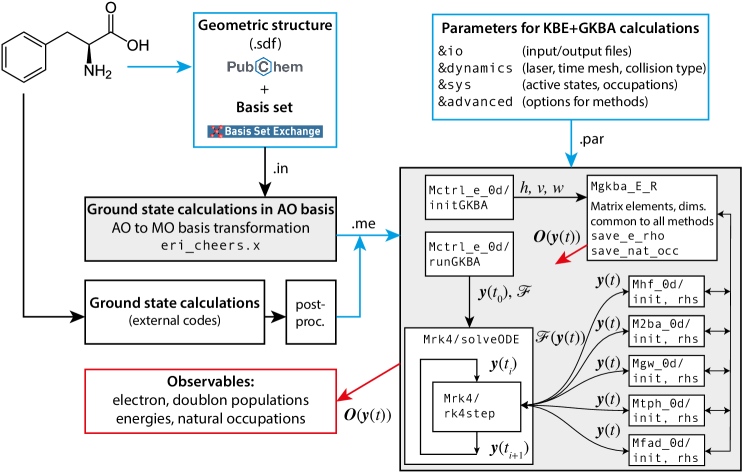
Figure 1: Workflow diagram of the GKBA+ODE calculations of the nonequilibrium dynamics in molecular systems (one can think of them as zero dimensional systems, and this is reflected in suffixes _0d in the names of respective modules). Pieces of code belonging to the cheers package are gray-shaded. Input parameters are framed in blue color, output observables are framed in red color. Most computationally intensive subroutines are rhs belonging to the modules Mhf, M2ba, Mgw, Mtph, Mtpp, and Mfad. They all have access to the module Mgkba_E_R, which contains all relevant system parameters needed for the time-propagation. Mrk4 is our implementation of the RK4 algorithms. It contains a stepper rk4step and a driver solveODE, which loops over the times, estimates propagation error and calls a subroutine for the computation of observables. Due to its simplicity and efficiency rk4step is not parallelized, whereas rhs are perfect candidates for parallelization.

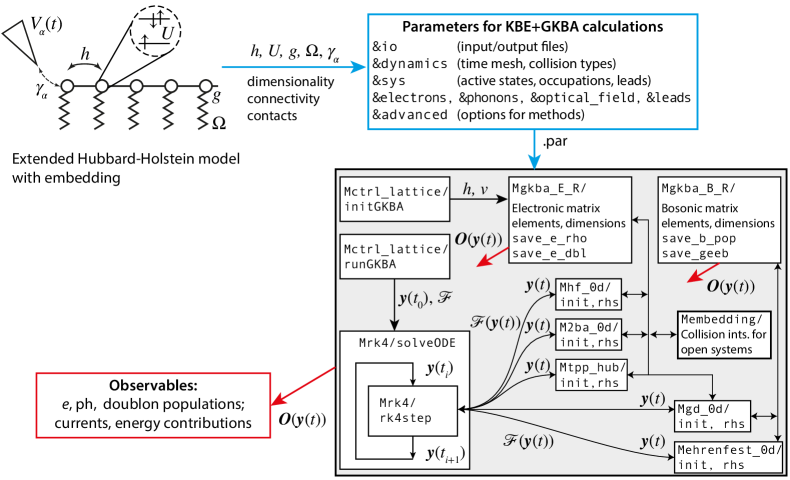
Figure 2: Workflow diagram of the GKBA+ODE calculations of the nonequilibrium dynamics in model lattice systems. Notations as in Fig. 1. Additionally we have a module for storing bosonic variables Mgkba_B_R and computational bosonic modules Mehrenfest_0d and Mgd_0d. Notice that electronic and bosonic modules are not completely independent. For instance Mgd_0d needs to fetch effective electronic one-body Hamiltonian stored in Mgkba_E_R.

We focus on the scenario where several copies of the state vector $\bm{\mathit{y}}(t)$ can be stored in the main memory of a computer or be distributed to each node of a computer cluster. This is by no means obvious: typical DFT implementations completely avoid the storage of quantities scaling as a forth power of the system size (such as Coulomb integrals). They operate with one-body densities with quadratic scaling, whereas the Coulomb matrix elements in atomic orbital (AO) basis are computed “on the fly”, allowing one to perform self-consistent calculations even for proteins [37].

This approach is not feasible for a KBE+GKBA theory, which is often formulated in the molecular orbital (MO) basis making the re-computation of the Hamiltonian matrix elements at each time-step infeasible. Intricacies of the basis selection and the basis transformation are discussed by [21], where it is shown how to deal with a continuum of unbound states that participate in the photoionization processes. This constitutes a separate preparatory step. Of course, the fact that $N_{v}=\mathcal{O}\left(N_{\text{$e$-basis}}^{4}\right)$ puts strong restrictions of the feasible system sizes. Let us consider a few representative examples (Tab. 1). As can be seen from the table, the number of atomic basis functions in the full-electron calculations is significantly larger than the number of occupied and virtual MO states used in the GKBA+ODE dynamics. This is achieved by excluding the core and the unoccupied states with large positive energy. This restriction is not mathematically but physically motivated considering typical optical excitations using an XUV laser. For instance, in  [29] we performed calculations for the Glycine molecule using only 5 relevant valence states out of 15 available. This selection was based on the insight provided by experimental measurements [38] and theoretical calculations [39, 40].

As a rule, in our calculations we use experimental molecular geometries from the PubChem [41] online database and Gaussian basis sets from the Basis Set Exchange [42] online resource. We note, however, that cheers is not restricted to this scenario, it is conceptualized to work with any programs that can generate MO integrals (Fig. 1) as well as with model systems (Fig. 2). In order to get familiar with the second possibility, in Tab. 2 we present typical resources in order to study the electron localization [43] in the Hubbard-Holstein model. A novel feature of these calculations is that both $e$-$e$ and $e$-ph interactions are taken into account.

Table 2: Largest systems and computational resources (Xeon Gold 5218 CPU @ 2.30GHz) required to study the dynamics of the Holstein-Hubbard model with $N$ sites and physical propagation time $t_{\text{f}}$. We compare timings and sizes of the state vector for a set of electronic (HF — Hartree-Fock, 2B — second Born, $T^{pp}$ — $T$-matrix in the particle-particle channel) and bosonic (Ehrenfest — mean-field, $GD$ — Fan-Migdal approximation) methods.

System	Correlations		State	Time	CPU hours
$N$	$e$-$e$	$e$-ph	vector	$t_{\text{f}}$	$e$-$e$	$e$-ph
151	HF	Ehrenfest	23 254	40	0.02	0.07
151	HF	$GD$	7 046 264	40	3.8	2.0
151	2B	$GD$	526 954 666	40	181.2	2.0
151	$T^{pp}$	Ehrenfest	519 931 656	40	482.8	0.04
151	$T^{pp}$	$GD$	526 954 666	40	488.0	2.6

It can be concluded on the basis of these two examples that GKBA+ODE calculations are routinely possible for amino acid molecules and correlated 1D clusters. From the structure of the code depicted in Figs. 1, 2, the separation of the ODE solver from the data generation and the RHS evaluation ($\mathcal{F}\left\{t,\bm{\mathit{y}}(t)\right\}$) represents an optimal architecture amenable to different parallelizations. It is anticipated that our code can be applied to a variety of physical scenarios, including ultrafast charge migration in XUV photoexcited halogenated amino acids [44], 2D and 3D model systems. In the next sections we consider some representative blocks of code according to the workflow diagrams. More detailed description of the full structure is deferred to the Supporting Information.

2.2 Ground state properties and the initialization of the ODE solver

Let us start with molecular systems. As can be seen from the workflow in Fig. 1, a ground state calculation is required in order to generate matrix elements for subsequent propagation. They are stored in a binary format in the file with an extension .me containing the following records:

me1p

One-particle matrix elements. They typically comprise the kinetic energy operator, electron-nuclear repulsion and the mean-field interaction of valence electrons with the core electrons. Depending on the method, core electrons may or may not be included in the ground state calculation. The active space for dynamical calculations is determined by physical considerations.

medp

Dipole transition matrix elements along three Cartesian axes.

me2p

Two-particle matrix elements representing the Coulomb repulsion between the electrons.

Matrix elements are assumed to be real and they are stored in a packed form in accordance with their symmetries. One of the first tasks is to read the matrix elements (me1p, medp, me2p) and the system dimensions (the number of electronic states NP and highest occupied molecular orbital NF) and store them in the Msys_0d module. We typically assume that HF Hamiltonian is diagonal in MO basis. This is dictated by practical rather than physical considerations: for instance one may study correlated molecular dynamics starting from a weakly correlated ground state in which the initial density matrix is diagonal and stationary.

However, cheers is not limited to molecular systems. Correspondingly, there are several Msys_ modules. Information on the lattice systems is stored in the Msys_lattice module, whereas for restricted Hartree-Fock calculations in atomic basis, the eri_cheers.x program (part of cheers) makes use of the Msys_molecule module to store the information about the AO-basis.

The second input file, which is mandatory for all GKBA+ODE calculations, is a parameter file .par. It consists of several namelists reflecting different aspects of a simulation:

io

provides names of the matrix elements file and output files for observables.

dynamics

specifies the propagation time-interval, time-step, and the level of treatment of electronic and bosonic correlations. Currently, only a fixed time-step ODE solver is used. Although it may not be the fastest option, this choice ensures that calculations remain reproducible and directly comparable to other codes, thereby simplifying the debugging process.

sys

gives MO basis size, index of highest occupied molecular orbital, and dimensionality, number of orbitals per site, number of leads for lattice systems. The number of read MO states (np) may in general be different (smaller or equal) from the number of MO states in the .me file. Also, np may in general be different (greater or equal) from the size of electronic basis for the GKBA+ODE calculations, $N_{\text{$e$-basis}}$ (ns). This gives one additional flexibility to experiment with different sets of active molecular orbitals and to exclude irrelevant valence states from the consideration (known in advance to be always occupied or always empty).

electrons

provides details of electron hopping (nearest and next-nearest) and Coulomb interaction, periodicity, spinless option, and extension for lattice systems. The resulting electronic quantities are then stored in Mgkba_E_R. This is one of the most important modules as it contains all the data for electronic GKBA+ODE calculations. As is depicted in Fig. 1, the computational routines in Mhf, M2ba, Mgw, Mtph, Mtpp, and Mfad make use of the matrix elements stored in Mgkba_E_R and also use the module for intermediate quantities.

phonons

gives phononic frequencies and parameters of $e$-ph interaction. Based on them, corresponding matrix elements are constructed and stored in the Mgkba_B_R module. The computational routines in the bosonic modules Mehrenfest_0d and Mgd_0d make use of the matrix elements and also use the module for the storage of intermediate quantities.

optical_field

contains parameters of the laser pulses, such as duration, frequency and shape.

leads

contains tunneling rate matrices for the wide band limit approximation (WBLA), or details of the leads and tunneling Hamiltonians;

advanced

specifies additional options for the methods used, such as, inclusion of exchange, freezing of mean field Hamiltonians, presence of acoustic phonons, treatment of Coulomb integrals with two indices or as complex quantities. Each of the methods may have different options, all the possibilities are described in Moptions.

2.3 Organization of the state vector

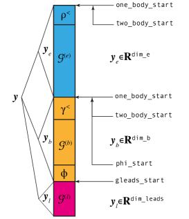
Figure 3: Organization of the state vector. Electronic, bosonic and leads part with dimensions dim_e, dim_b, and dim_l, respectively, are indicated with different colors. In the electronic part the electron density matrix $\rho^{<}$ (Eq. 15) and two-electron correlator $\mathcal{G}^{e}$ (Eq. 17) can be accessed at off-sets one_body_start and two_body_start, respectively. In the bosonic part, the bosonic density matrix $\gamma^{<}$ (Eq. 18), electron-boson correlator $\mathcal{G}^{b}$ (Eq. 21), and expectation values of bosonic field operators $\phi$ (Eq. 22) can be accessed at off-sets one_body_start, two_body_start and phi_start, respectively. Finally, the embedding correlator $\mathcal{G}^{\text{em}}$ (Eq. 23) can be found at the off-set gleads_start.

The code comprises several executables (such as shown in Figs. 1, 2). Therefore, the state vector $\bm{\mathit{y}}$ is physically located in different modules Mctrl_e_0d (molecular systems), Mctrl_lattice (lattice systems) and in Mctrl_transport (lattice systems with embedding). It always contains the electronic component, and can optionally contain the phononic (or bosonic) and embedding (or leads) parts, i.e.,

$$\bm{\mathit{y}}(t) =\{\bm{\mathit{y}}_{e}(t),\bm{\mathit{y}}_{b}(t),\bm{\mathit{y}}_{l}(t)\},$$ (3)

as depicted in Fig. 3. In order to properly define each component, let us consider the most general system Hamiltonian.

System Hamiltonian

$$\hat{H}(t)=\hat{H}_{\text{el}}(t)+\hat{H}_{\text{bos}}(t)+\hat{H}_{\text{el-bos}}(t)+\hat{H}_{\text{leads}}+\hat{H}_{\text{tunnel}}.$$ (4)

It contains the electronic part

$$\hat{H}_{\text{el}}(t) =\sum_{ij}h_{ij}(t)\hat{d}_{i}^{\dagger}\hat{d}_{j}+\frac{1}{2}\sum_{ijmn}v_{ijmn}(t)\hat{d}_{i}^{\dagger}\hat{d}_{j}^{\dagger}\hat{d}_{m}\hat{d}_{n},$$ (5)

comprising a one-body term ($h^{\dagger}=h$) accounting for the kinetic energy as well as the interaction with nuclei and possible external fields. The time-dependence of $h_{ij}(t)=h^{0}_{ij}+\langle i|V_{\rm gate}(t)+\hat{\mathbf{d}}\cdot{\mathbf{E}_{\rm pulse}}(t)|j\rangle$ is due to a time-dependent gate voltage $V_{\mathrm{gate}}(t)$ and to a possible laser pulse $\mathbf{E}_{\rm pulse}(t)$ coupled to the electronic dipole operator $\hat{\mathbf{d}}$. Furthermore, there is a two-body term accounting for the Coulomb interaction between the electrons. The time-dependence of the Coulomb matrix elements $v_{ijmn}(t)=v_{ijmn}s(t)$ could be due to the adiabatic switching protocol $s(t)$ adopted to generate a correlated initial state. Latin indices denote one-electron states comprising orbital and spin degrees of freedom, i. e., $i=(\bm{i},\sigma)$. As can be seen from Figs. 1, 2, $h$ and $v$ matrix elements are stored in the Mgkba_E_R module.

We write the bosonic Hamiltonian as

$$\hat{H}_{\text{bos}}(t)=\sum_{\mu\nu}\Omega_{\mu\nu}(t)\hat{\phi}_{\mu}\hat{\phi}_{\nu},$$ (6)

where $\Omega^{\dagger}=\Omega$ may depend on time, such as in the parametric phonon drivings [45] setup. The annihilation and creation operators for a bosonic mode $\mu$, i.e., $\hat{a}_{\mbox{\scalebox{0.7}{$\scriptscriptstyle\mbox{\boldmath$\mu$}$}}}$ and $\hat{a}^{{\dagger}}_{\mbox{\scalebox{0.7}{$\scriptscriptstyle\mbox{\boldmath$\mu$}$}}}$, are arranged into a vector $(\hat{x}_{\mbox{\scalebox{0.7}{$\scriptscriptstyle\mbox{\boldmath$\mu$}$}}},\hat{p}_{\mbox{\scalebox{0.7}{$\scriptscriptstyle\mbox{\boldmath$\mu$}$}}})$ where $\hat{x}_{\mbox{\scalebox{0.7}{$\scriptscriptstyle\mbox{\boldmath$\mu$}$}}}=(\hat{a}^{{\dagger}}_{\mbox{\scalebox{0.7}{$\scriptscriptstyle\mbox{\boldmath$\mu$}$}}}+\hat{a}_{\mbox{\scalebox{0.7}{$\scriptscriptstyle\mbox{\boldmath$\mu$}$}}})/\sqrt{2}$ are the position operators and $\hat{p}_{\mbox{\scalebox{0.7}{$\scriptscriptstyle\mbox{\boldmath$\mu$}$}}}=i(\hat{a}^{{\dagger}}_{\mbox{\scalebox{0.7}{$\scriptscriptstyle\mbox{\boldmath$\mu$}$}}}-\hat{a}_{\mbox{\scalebox{0.7}{$\scriptscriptstyle\mbox{\boldmath$\mu$}$}}})/\sqrt{2}$ are the momentum operators. The greek index $\mu=(\mbox{\boldmath$\mu$},\xi)$ is then used to specify the bosonic mode and the component of the vector: $\hat{\phi}_{\mu}=\hat{x}_{\mbox{\scalebox{0.7}{$\scriptscriptstyle\mbox{\boldmath$\mu$}$}}}$ for $\xi=1$ and $\hat{\phi}_{\mu}=\hat{p}_{\mbox{\scalebox{0.7}{$\scriptscriptstyle\mbox{\boldmath$\mu$}$}}}$ for $\xi=2$. The electronic and bosonic subsystems interact through

$$\hat{H}_{\text{el-bos}}(t) =\sum_{\mu,ij}g_{\mu,ij}(t)\hat{d}_{i}^{\dagger}\hat{d}_{j}\hat{\phi}_{\mu};$$ (7)

therefore electrons can be coupled to both the mode coordinates and momenta. We allow $g$ to depend on time for possible adiabatic switchings, i. e., $g_{\mu,ij}(t)=g_{\mu,ij}s(t)$. $\Omega$ and $g$ matrix elements are stored in the Mgkba_B_R module.

Similarly to the bosonic part, the lead part of the total Hamiltonian is optional: not every calculation is performed with transport setup in mind, moreover the leads and the tunneling Hamiltonian parts do not explicitly enter the formalism in the wide-band limit approximation. Nonetheless, we provide some possible explicit forms of these parts in order to give a microscopic definition of the tunneling-rate matrices. Thus, the leads Hamiltonian can be parametrized as

$$\hat{H}_{\text{leads}} =\sum_{k,\alpha,\sigma}\epsilon_{k\alpha}\hat{c}_{k\alpha,\sigma}^{\dagger}\hat{c}_{k\alpha,\sigma}.$$ (8)

At the moment we assume one-dimensional momenta $k$. Here $\alpha$ denotes the lead number and $\sigma$ is the spin projection. For a one-dimensional tight-binding chain (with on-site energy $a_{\alpha}$ and hopping $b_{\alpha}$) the electron energy dispersion $\epsilon_{k\alpha}$ is parametrized as

$$\epsilon_{k\alpha,\sigma} =a_{\alpha}+2|b_{\alpha}|\cos\left(\frac{k\pi}{N_{k}+1}\right), 1 \leq k\leq N_{k}.$$ (9)

As can be seen, $a$ and $b$ are lead-dependent, whereas we assume the same number of momenta $N_{k}$ per each lead. Here, leads are not spin-polarized, but it would be straightforward to consider, e. g., ferromagnetic leads via modified lead energies. Upon the application of a time-dependent bias voltage $V_{\alpha}(t)$, the lead energies are modified as

$$\tilde{\epsilon}_{k\alpha,\sigma}(t) =\epsilon_{k\alpha,\sigma}+V_{\alpha}(t).$$ (10)

The tunneling Hamiltonian can be parametrized as:

$$\hat{H}_{\text{tunnel}}(t) =\sum_{k,\alpha}\sum_{\bm{i},\sigma}T_{\bm{i},k\alpha}(t)\left[\hat{d}_{\bm{i},\sigma}^{\dagger}\hat{c}_{k\alpha,\sigma}+h.c.\right].$$ (11)

The coupling strengths are in general time- and lead-dependent, but it is assumed that for each lead $\alpha$ there is a single contact site, i.e.,

$$T_{\bm{i},k\alpha}(t) =t_{\alpha}\delta_{\bm{i}C_{\alpha}}\sqrt{\frac{2}{N_{k}+1}}\sin\left(\frac{k\pi}{N_{k}+1}\right)s_{\alpha}(t).$$ (12)

$C_{\alpha}$ represents the quantum number (such as site number and band index) of the electronic state that couples to the lead $\alpha$. $s_{\alpha}(t)$ is the switch-on function between the system and the lead $\alpha$, see Fig. 2. Next we define the tunneling-rate matrix

$$\Gamma_{\alpha,\bm{ij}}(\omega;t) =2\pi\sum_{k=1}^{N_{k}}T_{\bm{i},k\alpha}(t)\delta(\omega-\epsilon_{k\alpha})T_{\bm{j},k\alpha}^{*}(t),$$ (13)

which is in general frequency-dependent, but in WBLA it reduces to

$$\Gamma_{\alpha,\bm{ij}}(\omega;t) =\gamma_{\alpha}\delta_{\bm{i}C_{\alpha}}\delta_{\bm{j}C_{\alpha}}s_{\alpha}^{2}(t).$$ (14)

Parts of the state vector

The electronic component $\bm{\mathit{y}}_{e}$ contains i) the electron density matrix

$$\rho_{ij}^{<} =-iG^{<}_{ij}(t,t),$$ (15)

$$G^{<}_{ij}(t,t^{\prime}) =i\langle\hat{d}^{\dagger}_{j}(t^{\prime})\hat{d}_{i}(t)\rangle,$$ (16)

proportional to the equal-time lesser Green’s function $G^{<}$; and ii) a two-electron correlator

$$\mathcal{G}^{e}_{imjn}(t) =-\langle\hat{d}^{{\dagger}}_{n}(t)\hat{d}^{{\dagger}}_{j}(t)\hat{d}_{i}(t)\hat{d}_{m}(t)\rangle_{c},$$ (17)

The subscript “$c$” in the averages signifies that only the correlated part must be retained.

The bosonic component $\bm{\mathit{y}}_{b}$ contains i) the bosonic density matrix $\gamma^{<}_{\mu\nu}$

$$\gamma_{\mu\nu}^{<}(t) =iD^{<}_{\mu\nu}(t,t),$$ (18)

$$D^{<}_{\mu\nu}(t,t^{\prime}) =D^{>}_{\nu\mu}(t^{\prime},t)=-i\langle\Delta\hat{\phi}_{\nu}(t^{\prime})\Delta\hat{\phi}_{\mu}(t)\rangle,$$ (19)

$$\Delta\hat{\phi}_{\nu}(t) \equiv\hat{\phi}_{\nu}(t)-\langle\hat{\phi}_{\nu}(t)\rangle,$$ (20)

proportional to the equal-time lesser bosonic Green’s function $D^{<}_{\mu\nu}$; ii) a higher-order electron-boson correlator

$$\mathcal{G}^{b}_{\mu,ij}(t) =\langle\hat{d}^{{\dagger}}_{j}(t)\hat{d}_{i}(t)\hat{\phi}_{\mu}(t)\rangle_{c},$$ (21)

and iii) the expectation values of the bosonic field operators:

$$\phi_{\nu}(t) \equiv\langle\hat{\phi}_{\nu}(t)\rangle.$$ (22)

Matrices $\gamma^{<}$, $D^{<}$ have dimensions $N_{\text{$b$-basis}}\times N_{\text{$b$-basis}}$.

To deal with open systems, the leads part $\bm{\mathit{y}}_{l}$ contains the embedding correlator $\mathcal{G}^{\text{em}}$, which can be completely specified in terms of the leads and tunneling Hamiltonians, together with the quasi-particle propagators of the coupled system. This is due to the leads being non-interacting and in contrast to other higher-order correlators such as Eq. (17). Here, we consider the wide-band limit approximation by expressing the embedding correlator within the so-called pole expansion scheme [31],

$$\mathcal{G}_{l\alpha}^{\text{em}}(t)=\int d\bar{t}s_{\alpha}(\bar{t}){\rm e}^{-i\phi_{\alpha}(t,\bar{t})}{\rm e}^{-i\mu(t-\bar{t})}{\rm e}^{-\zeta_{l}(t-\bar{t})/\beta}G^{\text{A}}(\bar{t},t).$$ (23)

While we will next specify all the components of Eq. (23), we refer the Reader to the Supporting Information and our recent letter [31] for additional details. The embedding correlator, besides depending on the lead index $1\leq\alpha\leq N_{\text{leads}}$ contains the dependence on the pole index $1\leq l\leq N_{p}$ in the expansion of the Fermi distribution function

$$f(x)=\frac{1}{{\rm e}^{\beta x}+1} =\frac{1}{2}-\lim_{N_{p}\to\infty}\sum_{l=1}^{N_{p}}\eta_{l}\left(\frac{1}{\beta x+i\zeta_{l}}+\frac{1}{\beta x-i\zeta_{l}}\right),$$ (24)

where $\eta$ and $\pm i\zeta$ are the residues and poles ($\zeta>0$), respectively. We typically use the expansion coefficients generated by solving an eigenvalue problem of a specific, tridiagonal matrix [46]. Additionally $\phi_{\alpha}(t,t^{\prime})$ is the bias-voltage phase factor

$$\phi_{\alpha}(t,t^{\prime}) \equiv\int_{t^{\prime}}^{t}d\bar{t}V_{\alpha}(\bar{t}),$$ (25)

$\mu$ is the chemical potential, and

$$G^{\text{R}/\text{A}}(t,t^{\prime})=\mp i\theta[\pm(t-t^{\prime})]\mathrm{T}{\rm e}^{-i\int_{t^{\prime}}^{t}d\bar{t}h_{\text{eff}}^{e}(\bar{t})}$$ (26)

are the quasiparticle retarded/advanced propagators of the coupled system. Notice, that at variance with closed systems, the effective Hamiltonian is in general non-self-adjoint

$$h_{\text{eff}}^{e}(t) =h^{e}(t)-\frac{i}{2}\sum_{\alpha}\Gamma_{\alpha}s_{\alpha}^{2}(t)=h^{e}(t)-\frac{i}{2}\Gamma(t).$$ (27)

Matrices $h^{e}$, $\Gamma$, $G^{\text{R}/\text{A}}$, $\mathcal{G}_{l\alpha}^{\text{em}}$ have dimensions $N_{\text{$e$-basis}}\times N_{\text{$e$-basis}}$. We conclude this section by defining the mean-field electronic Hamiltonian

$$h^{e}_{ij}(t) =h_{ij}(t)+V^{\rm HF}_{ij}(t),$$ (28)

$$V^{\rm HF}_{ij}(t) =\sum_{mn}w_{imnj}\rho^{<}_{nm}(t),$$ (29)

with $w_{imnj}=v_{imnj}-v_{imjn}$ being the antisymmetrized interaction. The storage space for $\bm{\mathit{y}}$ — $\mathcal{O}(N_{v})$ — is dominated by the $\mathcal{G}^{e}$ correlator — $\mathcal{O}(N_{\text{$e$-basis}}^{4})$, the electron-boson correlator $\mathcal{G}^{b}$ — $\mathcal{O}(N_{\text{$e$-basis}}^{2}N_{\text{$b$-basis}})$, and the embedding correlator — $\mathcal{O}(N_{\text{$e$-basis}}^{2}N_{\text{leads}}N_{p})$, where $N_{\text{$b$-basis}}$ is double of the number of bosonic modes, and the number of poles in the expansion of the Fermi distribution function is typically below 50.

2.4 Computational subroutines

In the previous section we introduced the electronic, bosonic and leads parts of the state vector. Equations of motion covering the combinations of electronic-bosonic and electronic-leads degrees of freedom were derived in Ref. [33] and Ref. [31], respectively. These equations demonstrate the conserving properties [30] and symmetries of underlying theories. It follows, for instance, that density matrices $\rho^{<}$ (Eq. 15) and $\gamma^{<}$ (Eq. 18) are self-adjoint and that higher-order correlators can be likewise written in matrix form, by combing electronic indices in pairs. From the electronic correlator tensor $\mathcal{G}^{e}_{imjn}$ (Eq. 17) a matrix $\bm{\mathcal{G}}^{e}(t)$ can be constructed in three different ways depending on the approximation used: $GW$, $T^{ph}$, or $T^{pp}$. These approximations contain an infinite sequence of diagrams corresponding to the solution of the Bethe-Salpeter equation in three different channels. $GW$ approximation corresponds to the treatment of $\overline{ph}$ channel, $T^{pp}$ approximation — $pp$ channel, and $T^{ph}$ — $ph$ channel, where we refer to the naming convention used in the parquet theory [47]. Additionally, it is possible to take even more complicated diagrams into account by including exchange contributions [33]. In every such form the matrix $\bm{\mathcal{G}}^{e}(t)$ can be shown to be self-adjoint [29]. This matrix form of the GKBA+ODE method leads to important simplifications of the resulting equations, for instance only the upper triangular parts must be computed. For the explicit form of the equations we refer to corresponding papers [33, 31] and focus here more on their general functional form.

The evaluation of $\mathcal{F}\left\{t,\bm{\mathit{y}}(t)\right\}$ in Eq. (1a), which constitutes the main computational task, can be partitioned as

$$\mathcal{F}\left\{t,\bm{\mathit{y}}(t)\right\} =\left\{\mathcal{F}_{e}\left\{t,\bm{\mathit{y}}_{e}(t),\bm{\mathit{y}}_{b}(t),\bm{\mathit{y}}_{l}(t)\right\},\mathcal{F}_{b}\left\{t,\bm{\mathit{y}}_{e}(t),\bm{\mathit{y}}_{b}(t)\right\},\mathcal{F}_{l}\left\{t,\bm{\mathit{y}}_{e}(t),\bm{\mathit{y}}_{l}(t)\right\}\right\}.$$ (30)

As can be seen from this form, the evaluation of one part requires the knowledge of other parts. This structure is present even at the mean-field level, where the equation of motion for the bosonic and leads correlators depends on the electron density matrix. In correlated cases, there are feedbacks of these degrees of freedom on electrons, and the electron density matrix $\rho^{<}$ enters the evaluation of the higher-order correlators. These complicated relations are shown as arrows in Figs. 1, 2. The subroutines implementing different electronic, bosonic and embedding approximations are grouped in modules such as:

Mhf_0d

mean-field for electrons,

M2ba_0d

second Born approximation for electrons,

Mgw_0d and Mgw_hub

$GW$ approximation for molecular and lattice systems,

Mtpp_0d and Mtpp_hub

$T^{pp}$ approximation for molecular and lattice systems,

Mtph_0d and Mtph_hub

$T^{ph}$ approximation for molecular and lattice systems,

Mfad_0d

three-particle Faddeev method for molecular systems,

Mehrenfest_0d and Mgd_0d

Ehrenfest and Fan-Migdal (or $GD$) approximation for phonons,

Membedding

the spectral decomposition and the pole expansion methods for leads.

In addition to the state vector, the rhs subroutines (computing right hand sides of the equations of motion) in these modules rely on the common data (matrix elements) stored in Mgkba_E_R and Mgkba_B_R modules. The code is organized in such a way that subroutines implementing different approximations are completely interchangeable. For instance, every evaluation starts with a transformation between the state vector (real) $\bm{\mathit{y}}$ and the matrix form (complex) of $\rho^{<}$, $\bm{\mathcal{G}}^{e}(t)$ for electrons, $\gamma^{<}$, $\bm{\mathcal{G}}^{b}(t)$, $\phi$ for bosons, and $\mathcal{G}^{\text{em}}$ for leads. This computational overhead is needed for three reasons: i) simplicity and universality of the differential equation solver solveODE; ii) speed-up due to automatic loops unrolling in the Runge-Kutta algorithm, rk4step; iii) the computational complexity of the transformation operations is well below time-critical operations, which scale as fifth or higher power of the system size. There is also small memory saving due to the use of symmetry, which may play an important role in distributed computing. Therefore, it is possible to achieve a great variety of methods without code duplication. The details of this design are presented in Supporting Information. Let us now demonstrate the interplay of electronic correlations, electron-phonon interaction and tunneling to the leads in a model calculation.

3 Illustrative example

We consider here a 1D Hubbard model at low filling interacting at every site with a phonon mode. This is also known as the Holstein-Hubbard model, which is often studied in the context of polaron formation and electron localization [43] and field-driven heating [48]. We add here another aspect to these studies, namely the presence of leads connected to the two terminal sites ($N_{\text{leads}}=2$). This designates our model as a prototype for a photovoltaic device encompassing the phenomena of creation of nonequilibrium carriers, formation of the polaronic quasiparticles, and charge transport through the active material to leads. We focus here only on modelling of the conduction band. A realistic model of the whole photovoltaic device should also comprise the valence band, from where the electrons are excited, and the optical pulse. This calculation is fully within the capability of the code. However, here we deal with a simpler one-band scenario and perform calculations for shorter chains as compared to previous studies [34] — only 35 sites ($N_{v}=1792350$) — but they capture all relevant physical phenomena. As a benefit, all the calculations can be performed on a typical laptop within five minutes time. The Hamiltonian is given by

$$\hat{H}_{\text{h-h}} =-t_{\text{nn}}\sum_{\sigma=\uparrow,\downarrow}\sum_{<\bm{i},\bm{j}>}\hat{d}_{\bm{i}\sigma}^{\dagger}\hat{d}_{\bm{j}\sigma}+U\sum_{\bm{i}}\hat{n}_{\bm{i}\uparrow}\hat{n}_{\bm{i}\downarrow}+\sum_{\bm{i}}\left\{\Omega\hat{a}^{\dagger}_{\bm{i}}\hat{a}_{\bm{i}}+g(\hat{a}^{\dagger}_{\bm{i}}+\hat{a}_{\bm{i}})\hat{n}_{\bm{i}}\right\},$$ (31)

where $\hat{n}_{\bm{i}}=\sum_{\sigma}\hat{n}_{\bm{i}\sigma}$, $\hat{n}_{\bm{i}\sigma}=\hat{d}_{\bm{i}\sigma}^{\dagger}\hat{d}_{\bm{i}\sigma}$, and we set $t_{\text{nn}}=\Omega=1$, and $U=2$, $g=0.5$. The dynamics is triggered by the creation of an electron pair at the central lattice site. Initially the lattice is empty. In the absence of leads the electronic wave packet spreads on the lattice, whereby the electron group velocity is at most $2t_{\text{nn}}$. Two electrons occupying the same lattice site form a doublon, a long-living excitation, the decay of which is suppressed by energy conservation. Its group velocity is in general different from the electronic one and in the strongly interacting limit can be estimated as $4t_{\text{nn}}^{2}/U$. Propagation of electrons and doublons at low filling can be accurately described by the $T^{pp}$ approximation [34]. Both velocities are renormalized by the $e$-ph interaction.

If such a system is subject to open boundary conditions, the electronic wave-packet will hit the chain boundaries and reflect after propagating for a certain time. If the system is connected to leads, the charge will tunnel into or from the central region, and the number of electrons in the system will not be preserved. In the present scenario, we study how $e$-$e$ and $e$-ph interactions influence the charge flow to leads in the wide band limit approximation. The chemical potential of the leads and central system is assumed to be equal, however, we set the lead voltage to a large negative value ($V_{\alpha}=-5$). This enables electrons to leave the chain. The dynamics of the system can be understood based on the analysis of total populations in Fig. 4.

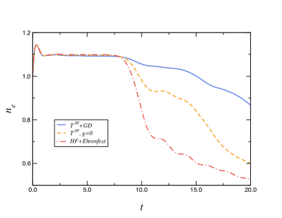
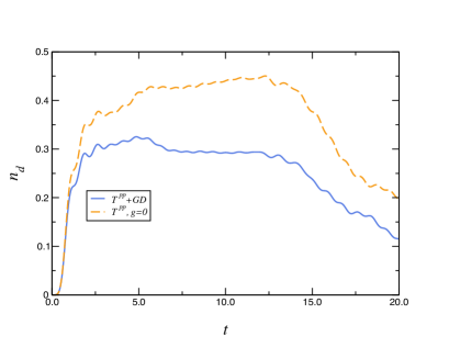
Figure 4: Total number of electrons and doublons in a 35-sites system connected to leads with $V_{\alpha}=-5$, $\gamma_{\alpha}=1$, and $\beta=100$. Different line-styles denote different levels of treatment of $e$-$e$ and $e$-ph interactions. Electrons are characterized by the nearest-neighbor hopping $t_{\text{nn}}=1$ and on-site Hubbard interaction $U=2$. The phonon frequency is set to $\Omega=1$, and the electron-phonon coupling constant for calculations within the Fan-Migdal approach (blue solid lines) or the Ehrenfest approach (red dash-dotted line) is set to $g=0.5$. The orange dashed line denotes results without the electron-phonon interaction ($g=0$). Electrons are treated either at the Hartree-Fock (HF) or the $T$-matrix in the particle-particle channel level of approximation.

The considered system is not spin polarized. Therefore, only the spatial components of $\rho^{<}$ and $\mathcal{G}^{e}$ are propagated. They are defined as

$$\rho_{\bm{\mathit{i}}\bm{\mathit{j}}}^{<} \equiv\rho_{\bm{\mathit{i}}\sigma,\bm{\mathit{j}}\sigma}^{<},$$ (32)

$$\mathcal{G}^{e}_{\bm{\mathit{i}}\bm{\mathit{m}}\bm{\mathit{j}}\bm{\mathit{n}}} \equiv\mathcal{G}^{e}_{\bm{\mathit{i}}\sigma,\bm{\mathit{m}}\sigma,\bm{\mathit{j}}\sigma,\bm{\mathit{n}}\sigma},$$ (33)

where $\sigma=\uparrow,\downarrow$. The electronic and doublonic populations are defined then as respective diagonal elements

$$n_{\bm{\mathit{i}}} \equiv\langle\hat{n}_{\bm{\mathit{i}},\sigma}\rangle=\rho_{\bm{\mathit{i}}\bm{\mathit{i}}}^{<},$$ (34)

$$d_{\bm{\mathit{i}}} \equiv\langle\hat{n}_{\bm{\mathit{i}},\uparrow}\hat{n}_{\bm{\mathit{i}},\downarrow}\rangle-n_{\bm{\mathit{i}}}^{2}=-\mathcal{G}^{e}_{\bm{\mathit{i}}\bm{\mathit{i}}\bm{\mathit{i}}\bm{\mathit{i}}}.$$ (35)

Initially the total number of spin-up or spin-down electrons is

$$n_{e} =\sum_{\bm{\mathit{i}}}n_{\bm{\mathit{i}}}=1,$$ (36)

and the system is uncorrelated, therefore the number of doublons is zero

$$n_{d} =\sum_{\bm{\mathit{i}}}d_{\bm{\mathit{i}}}=0,$$ (37)

notice that uncorrelated part is subtracted in the definition of $d_{\bm{\mathit{i}}}$.

It is assumed that leads with $\gamma_{\alpha}=1$ and inverse temperature $\beta=100$ are attached suddenly at $t=0$, i. e., $s_{\alpha}(t)=\theta(t)$, as the propagation starts at $t_{i}=0$. Since the central system and the leads are initially not equilibrated, the relaxation gives rise to a small flow of charge in and out of the system at $t\simeq 0.5$. After this kink, $n_{e}$ remains constant, and the build up of $e$-$e$ and $e$-ph correlations takes place. This is reflected in the rapid growth of the doublon population, primarily driven by pure electronic scattering, and its oscillations resulting from interactions with phonons. Simultaneously, electrons and doublons propagate through the lattice with distinct group velocities until they reach the boundaries. It is important to note that the travel times for electrons and doublons are significantly different (compare the length of plateau in the plots of $n_{e}$ and $n_{d}$). After reaching the boundaries, electrons tunnel to the leads indirectly reducing the number of doublons in the system. The rate of tunneling strongly depends on the presence of phonons and on the level of approximation used. It can be seen, for instance, that $T^{pp}$ approximation for the electron and Fan-Migdal (or $GD$) approximation for the phonon self-energies, respectively, predicts the slowest decline of populations (smallest current). In the absence of $e$-ph coupling ($g=0$) electrons leak to the leads faster, whereas the mean-field treatment of both interactions, which does not capture the formation of bound doublon or polaron states, results in the fastest depletion of the central region.

4 Conclusions

We presented a NEGF toolbox for the simulation of the coupled electron-boson dynamics in correlated materials including the treatment of open systems with fermionic bath. The merits of our implementation in the cheers package are as follows: (1) all fundamental conservation laws are satisfied independently of the method [30]; (2) the ODE nature of the EOM allows one to address phenomena occurring at different time scales through a save-and-restart procedure; and (3) as a byproduct of the calculations we have access to the spatially nonlocal correlators $\bm{\mathcal{G}}^{e}(t)$ and $\bm{\mathcal{G}}^{b}(t)$, as well as to the embedding correlator $\mathcal{G}^{\text{em}}$ that allows evaluation of currents according to the Meir-Wingreen formula [31]. The ODE formulation naturally accommodates parallel computations, adaptive time-stepping implementations, and restart protocols, thereby paving the way for conducting first principles simulations of multiscale systems. As an illustration of our method, we investigated a 1D Holstein-Hubbard model in a setup corresponding to the conduction band of a photovoltaic device. We found that the formation of bound doublonic and polaronic states reduces the photo-current.

Supporting Information

Supporting Information is available from the Wiley Online Library or from the authors. At present, the code is given only for collaborative purposes. The interested reader can contact the authors of the code.

References

- [1] D. N. Basov, R. D. Averitt, D. Hsieh, Nat. Mater. 2017, 16, 11 1077.
- [2] G. Stefanucci, R. van Leeuwen, Nonequilibrium Many-Body Theory of Quantum Systems: A Modern Introduction, Cambridge University Press, Cambridge, 2013.
- [3] N.-H. Kwong, M. Bonitz, Phys. Rev. Lett. 2000, 84, 8 1768.
- [4] N. E. Dahlen, R. van Leeuwen, Phys. Rev. Lett. 2007, 98, 15 153004.
- [5] P. Myöhänen, A. Stan, G. Stefanucci, R. van Leeuwen, Eurphys. Lett. 2008, 84 67001.
- [6] M. Galperin, S. Tretiak, J. Chem. Phys. 2008, 128, 12 124705.
- [7] P. Myöhänen, A. Stan, G. Stefanucci, R. van Leeuwen, Phys. Rev. B 2009, 80, 11 115107.
- [8] M. P. von Friesen, C. Verdozzi, C.-O. Almbladh, Phys. Rev. Lett. 2009, 103, 17 176404.
- [9] N. Bittner, D. Golež, H. U. R. Strand, M. Eckstein, P. Werner, Phys. Rev. B 2018, 97, 23 235125.
- [10] M. Schüler, J. Berakdar, Y. Pavlyukh, Phys. Rev. B 2016, 93, 5 054303.
- [11] M. Schüler, D. Golež, Y. Murakami, N. Bittner, A. Herrmann, H. U. Strand, P. Werner, M. Eckstein, Comp. Phys. Commun. 2020, 257 107484.
- [12] J. Kaye, D. Golez, SciPost Physics 2021, 10, 4 091.
- [13] F. Meirinhos, M. Kajan, J. Kroha, T. Bode, SciPost Physics Core 2022, 5, 2 030.
- [14] X. Dong, E. Gull, H. U. R. Strand, Phys. Rev. B 2022, 106, 12 125153.
- [15] P. Lipavský, V. Špička, B. Velický, Phys. Rev. B 1986, 34, 10 6933.
- [16] E. V. n. Boström, A. Mikkelsen, C. Verdozzi, E. Perfetto, G. Stefanucci, Nano Lett. 2018, 18, 2 785.
- [17] F. Covito, E. Perfetto, A. Rubio, G. Stefanucci, Phys. Rev. A 2018, 97, 6 061401(R).
- [18] S. Latini, E. Perfetto, A.-M. Uimonen, R. van Leeuwen, G. Stefanucci, Phys. Rev. B 2014, 89, 7 075306.
- [19] E. P. Månsson, S. Latini, F. Covito, V. Wanie, M. Galli, E. Perfetto, G. Stefanucci, H. Hübener, U. De Giovannini, M. C. Castrovilli, et al., Commun. Chem. 2021, 4, 1 73.
- [20] E. Perfetto, D. Sangalli, A. Marini, G. Stefanucci, J. Phys. Chem. Lett. 2018, 9, 6 1353.
- [21] E. Perfetto, D. Sangalli, M. Palummo, A. Marini, G. Stefanucci, J. Chem. Theory Comput. 2019, 15, 8 4526.
- [22] E. Perfetto, A. Trabattoni, F. Calegari, M. Nisoli, A. Marini, G. Stefanucci, J. Phys. Chem. Lett. 2020, 9.
- [23] E. Perfetto, A.-M. Uimonen, R. van Leeuwen, G. Stefanucci, Phys. Rev. A 2015, 92, 3 033419.
- [24] E. Perfetto, Y. Pavlyukh, G. Stefanucci, Phys. Rev. Lett. 2022, 128, 1 016801.
- [25] E. Perfetto, G. Stefanucci, Nano Lett. 2023, 23, 15 7029.
- [26] E. Perfetto, G. Stefanucci, J. Phys. Condens. Matter 2018, 30, 46 465901.
- [27] N. Schlünzen, J.-P. Joost, M. Bonitz, Phys. Rev. Lett. 2020, 124, 7 076601.
- [28] J.-P. Joost, N. Schlünzen, M. Bonitz, Phys. Rev. B 2020, 101, 24 245101.
- [29] Y. Pavlyukh, E. Perfetto, G. Stefanucci, Phys. Rev. B 2021, 104, 3 035124.
- [30] D. Karlsson, R. van Leeuwen, Y. Pavlyukh, E. Perfetto, G. Stefanucci, Phys. Rev. Lett. 2021, 127, 3 036402.
- [31] R. Tuovinen, Y. Pavlyukh, E. Perfetto, G. Stefanucci, Phys. Rev. Lett. 2023, 130 246301.
- [32] Y. Meir, N. S. Wingreen, Phys. Rev. Lett. 1992, 68, 16 2512.
- [33] Y. Pavlyukh, E. Perfetto, D. Karlsson, R. van Leeuwen, G. Stefanucci, Phys. Rev. B 2022, 105, 12 125134.
- [34] Y. Pavlyukh, E. Perfetto, D. Karlsson, R. van Leeuwen, G. Stefanucci, Phys. Rev. B 2022, 105, 12 125135.
- [35] Y. Pavlyukh, J. Berakdar, Comp. Phys. Commun. 2013, 184 387.
- [36] J.-P. Joost, N. Schlünzen, H. Ohldag, M. Bonitz, F. Lackner, I. Březinová, Phys. Rev. B 2022, 105, 16 165155.
- [37] D. J. Cole, N. D. M. Hine, J. Phys. Condens. Matter 2016, 28, 39 393001.
- [38] R. Weinkauf, P. Schanen, A. Metsala, E. Schlag, M. Bürgle, H. Kessler, The Journal of Physical Chemistry 1996, 100, 47 18567.
- [39] A. I. Kuleff, J. Breidbach, L. S. Cederbaum, J. Chem. Phys. 2005, 123, 4 044111.
- [40] D. Ayuso, A. Palacios, P. Decleva, F. Martín, Phys. Chem. Chem. Phys. 2017, 19, 30 19767.
- [41] S. Kim, J. Chen, T. Cheng, A. Gindulyte, J. He, S. He, Q. Li, B. A. Shoemaker, P. A. Thiessen, B. Yu, L. Zaslavsky, J. Zhang, E. E. Bolton, Nucleic Acids Res. 2021, 49, D1 D1388.
- [42] B. P. Pritchard, D. Altarawy, B. Didier, T. D. Gibson, T. L. Windus, J. Chem. Inf. Model. 2019, 59, 11 4814.
- [43] B. Kloss, D. R. Reichman, R. Tempelaar, Phys. Rev. Lett. 2019, 123, 12 126601.
- [44] G. Bergamaschi, L. Lascialfari, A. Pizzi, M. I. Martinez Espinoza, N. Demitri, A. Milani, A. Gori, P. Metrangolo, Chem. Comm. 2018, 54, 76 10718.
- [45] Y. Murakami, N. Tsuji, M. Eckstein, P. Werner, Phys. Rev. B 2017, 96 045125.
- [46] J. Hu, R.-X. Xu, Y. Yan, J. Chem. Phys. 2010, 133 101106.
- [47] K. Held, In E. Pavarini, E. Koch, D. Vollhardt, A. I. Lichtenstein, editors, DMFT at 25: infinite dimensions: lecture notes of the Autumn School on Correlated Electrons 2014. Forschungszentrum Jülich, Zentralbibliothek, Verl, Jülich, 2014.
- [48] M. Weber, J. K. Freericks, Phys. Rev. Lett. 2023, 130, 26 266401.