T. M. Aliev
taliev@metu.edu.trPhysics Department, Middle East Technical University, 06531, Ankara, Turkey
A. Ozpineci
ozpineci@metu.edu.trPhysics Department, Middle East Technical University, 06531, Ankara, Turkey
Y. Sarac
yasemin.sarac@atilim.edu.trElectrical and Electronics Engineering Department,
Atilim University, 06836 Ankara, Turkey
Abstract
The upper limit of the branching ratio of the rare decay is obtained as by the LHCb. In the present work we study this decay within the light cone QCD sum rules employing the distribution amplitudes. At first stage, the form factors entering the decay are obtained. Next, using the results for the form factors the corresponding branching ratio for this decay is estimated to be . This value lies below the upper limit established by the LHCb collaboration. Our finding for the branching ratio is also compared with the results of the other theoretical approaches existing in the literature.
I Introduction
The exclusive weak decays of hadrons governed by the flavor-changing neutral current (FCNC) transitions are forbidden in the Standard Model (SM) at the tree level and occur only at the one-loop level. Consequently, these decays hold exceptional significance for testing the predictions of the SM at the loop level as well as looking for the evidence of new physics beyond the SM. These decay channels are strongly suppressed, and this makes their experimental investigation difficult.
The rare exclusive radiative decay induced by transition has not been observed experimentally yet, and the LHCb collaboration imposed an upper limit on its branching ratio, LHCb:2021hfz . This decay was investigated within different approaches, such as light-front quark model (Geng:2022xpn, ), relativistic quark-diquark model Davydov:2022glx , light cone QCD sum rules Olamaei:2021eyo ; Liu:2011ema using the baryon distribution amplitudes, and in the framework of SU(3) flavor symmetry Wang:2020wxn . The difference in the predictions obtained in the Refs. Olamaei:2021eyo ; Wang:2020wxn ; Geng:2022xpn ; Davydov:2022glx , which are below the experimental upper limit, and Liu:2011ema and especially the difference between the predictions of Refs. Olamaei:2021eyo and Liu:2011ema despite being obtained using the same framework and same distribution amplitudes (DA’s), require a more careful analysis of this decay channel. Therefore in this work, we investigate the decay in the framework of light cone QCD sum rules by using the DA’s of the heavy baryon. The light cone QCD sum rules method (LCSR) Braun:1997kw is an extension of the traditional QCD sum rules Shifman:1978bx , and one of the powerful approaches among nonperturbative methods that yields predictions consistent with the experimental observations. In the LCSR the operator product expansion (OPE) is conducted over the twist of the operators, rather than the dimension of the operators as in the traditional QCD sum rules.
The organization of the work is as follows. In the next section, the LCSR for the transition form factors responsible for the decay are obtained by using the light cone DA’s. Sec. III is devoted to the numerical analyses for the relevant form factors obtained in the previous section. Moreover, the corresponding branching ratio is attained using their numerical values. Discussions and our conclusion are presented in Sec. IV.
II Form factors for the decay in light cone QCD sum rules
The rare transition is described by the following effective Hamiltonian:
(1)
where is Fermi coupling constant, are the Wilson coefficients, and and are Cabibbo-Kobayashi-Maskawa matrix elements. The are the local operators whose explicit forms can be found in Ref. Davydov:2022glx . Since the penguin operator gives the main contribution to the transition, the effective Hamiltonian for this transition is given as
(2)
where we use from Ref. Davydov:2022glx . The amplitude of the considered transition is obtained from the matrix element of the Hamiltonian taken between the initial and final states, which requires calculating the matrix element between the baryon states which can be expressed in terms of the form factors. In this section, we provide the details of the light cone QCD sum rule calculations to obtain the form factors for the transition.
The basic object of the light cone QCD sum rules is the correlation function that sandwiches the time-ordered product of the interpolating current of the final baryon state and the weak transition current between the vacuum and the initial hadron state , i.e.
(3)
where is the time ordering operator. For the considered problem the form of the weak transition current is and is the interpolating current of the baryon
(4)
where and are color indices, , , and with representing the charge conjugation operator, is an arbitrary parameter.
In the light cone QCD sum rules method, the correlation function is calculated in terms of hadron and in terms of quark gluon degrees of freedom, respectively. After matching the results of both representations the desired sum rules for the physical quantities are obtained.
The hadronic representation of the correlation function is obtained by inserting a complete set of baryon states carrying the same quantum numbers as the interpolating current in Eq. (3) and isolating the pole term of the baryon we get
(5)
The first matrix element appearing in Eq. (5) is determined in standard way and given as
(6)
where and represent the residue and spinor of the baryon, respectively. The transition matrix element, , is parametrized by the set of form factors in the following way:
(7)
where is the mass of the heavy baryon.
In the considered problem the photon is real. Consequently, only two form factors, and , at point contribute to the decay. Therefore, in the next calculations, we concentrate on the computations of only the and form factors.
Substituting Eqs. (6) and (7) in the Eq. (5) and using the completeness relation the correlation function for the hadronic side becomes
(8)
in which is defined as .
The calculation of the correlation function for the QCD side proceeds as follows. Using the interpolating current for baryon and the weak transition explicitly and after contracting the -quark fields via Wick theorem, we obtain the correlation function as
(9)
where is the -quark propagator. The matrix element in Eq. (9), , is expressed in terms of the light-cone distribution amplitudes (DA’s) of baryon that have been studied in Ref. Ali:2012zza . Here we would like to note that the light-cone distribution amplitudes are obtained within the heavy quark effective theory. The relation between the heavy baryon state and the heavy baryon state in the heavy quark effective theory is given by . After these remarks, in Eq. (9) we make the replacement, , hence appears the following matrix element
(10)
This matrix element can be written in terms of baryon DA’s Ali:2012zza as
(11)
where is the heavy quark effective field coming from the replacement of heavy quark field , and
(12)
Here , , and are the DA’s with twist 2, 3, and 4, respectively. The light cone vectors and have the following forms:
(13)
and the DA’s are defined as
(14)
with , and being the total momentum of the light quarks.
Choosing the coefficients of the structures and for the QCD part of the correlation function we have
(15)
where represent the contributions coming from other structures, the function is defined as
(16)
and
(17)
Matching the coefficients of the structures written in the above equation explicitly, and , obtained in both hadronic and QCD sides, and performing the Borel transformation with respect to the variable , we attain the following desired sum rules for the form factors and :
(18)
where and represent the Borel transformed results obtained from the QCD side for the structures and , respectively. From Eq. (15) it follows that , hence . To obtain the results after Borel-transformation and continuum subtraction, we apply the master formula given as
(19)
where , and is the solution of the equation , where is the continuum threshold.
Using the matrix element given in the Eq.(7) the decay width of the rare radiative decay is
In the previous section, the sum rules for the form factors and at point are derived. In present section, we perform the numerical analyses of sum rules for the form factors. Moreover, using the obtained results for and we estimate the corresponding branching ratio.
The main input parameters for the LCSR are the distribution amplitudes (DA’s), which are the DA’s of baryon in our case. These DA’s were obtained in Ref. Ali:2012zza , and their expressions are
(21)
for which the values of the parameters , and are given in Ref. Ali:2012pn with , is the Gegenbauer polynomial, and
(22)
The values of the other input parameters are as follows: For the residue , we have used the result of Ref. Lee:2002jb obtained for with . In our analysis to get numerical values for we have used the numerical values of the condensates given in Ref. Lee:2002jb and the threshold and Borel parameters are varied in the ranges and , respectively. The parameters and are taken as Wang:2020mxk . The input parameters taken from PDG Workman:2022ynf are , , GeV, MeV, MeV, MeV, s.
The sum rules also contain following auxiliary parameters: Borel parameter, , threshold parameter and the parameter entering to the interpolating current. The continuum threshold is determined from the analyses of two-point QCD sum rules, namely its value is obtained from the condition that the mass sum rule reproduces the experimentally measured values within 10% accuracy. This analysis leads to the result . The working region of the is determined by demanding that the power corrections and the continuum contributions be suppressed compared to the leading twist-2 contribution. Taking these conditions into account, we obtain the following domain for this parameter: .
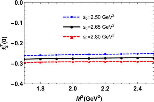
Using the DA’s for baryon given in Eq. (III), in Figure 1 the dependence of the form factor, , at zero momentum transfer squared on at fixed values of and , is presented. We see that the form factor, , exhibits good stability when varies in the working region, as can be seen.
Figure 1: Variation of the the form factor as function of at different values of threshold parameter and .
In order to find the working region of , in Figure 2 we present the dependence of on , where , at fixed values of and from their working regions. From this figure we observe that, when varies in the region , the form factor exhibits good stability on the variation of . Besides in this region the required criteria for Borel parameter, , and threshold parameter including the convergence of the OPE, are satisfied.
Figure 2: Variation of the the form factor as function of at fixed values of threshold parameter and Borel parameter in their working regions.
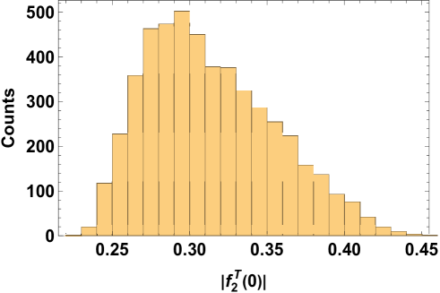
To analyze the stability of our predictions on all of the determined parameter space, the parameters, , , , and , are randomly selected inside the chosen region. The histogram of 5000 such computations are shown in Figure 3.
Figure 3: The histogram of the form factor obtained using arbitrary values of the auxiliary parameters, , , , and from their working intervals.
From these data the mean and the standard deviation of our predictions on the form factors are
(23)
Note that from the two-point sum rules results of Ref. Lee:2002jb , the sign of can not be predicted. Hence we only show the absolute values of the form factors at . Note also that the relative size of standard deviation is a measure of the stability of our predictions within the chosen region in the parameter space.
After the determination of the form factors, and , we can determine the decay width applying Eq. (20). Using the lifetime for baryon, s, we get the branching ratio as
(24)
At the end of this section we compare our result on branching ratio of with the existing results in literature and with the experimental upper bound, LHCb:2021hfz . The results are presented in the Table 1.
Table 1: The branching ratio, (BR), for obtained in different frameworks and the experimental upper bound.
From the table, it follows that the result of Ref. Liu:2011ema exceeds the predictions of all other works by one order and even exceeds the experimental upper limit. Our result has consistent order of magnitude with the results of all the works, except that of Ref. Liu:2011ema . The measurement of the branching ratio of decay may be useful for distinguishing the right picture.
IV Summary and conclusion
By using the heavy baryon distribution amplitudes the rare radiative decay is studied within the light cone QCD sum rules. The sum rules for the relevant form factors are derived and their numerical values are determined at point. Using the results of the form factors the branching ratio is estimated. Moreover, we perform a comparison between our finding and the results of other works in the literature on the branching ratio of decay. We obtained that the branching ratio, , has consistent order of magnitude with results given in Refs. Geng:2022xpn ; Davydov:2022glx ; Olamaei:2021eyo ; Wang:2020wxn and below the experimental upper limit LHCb:2021hfz . Besides, it is smaller than the result given in Ref. Liu:2011ema . Our final remark to this work is that the results presented here can be improved by taking into account corrections to the distribution amplitudes, as well as improving the values of parameters appearing in them.