Semantics of Attack-Defense Trees for Dynamic Countermeasures and a New Hierarchy of Star-free Languages

Abstract

We present a mathematical setting for attack-defense trees, a classic graphical model to specify attacks and countermeasures. We equip attack-defense trees with (trace) language semantics allowing to have an original dynamic interpretation of countermeasures. Interestingly, the expressiveness of attack-defense trees coincides with star-free languages, and the nested countermeasures impact the expressiveness of attack-defense trees. With an adequate notion of countermeasure-depth, we exhibit a strict hierarchy of the star-free languages that does not coincides with the classic one. Additionally, driven by the use of attack-defense trees in practice, we address the decision problems of trace membership and of non-emptiness, and study their computational complexities parameterized by the countermeasure-depth.

1 Introduction

Security is nowadays a subject of increasing attention as means to protect critical information resources from disclosure, theft or damage. The informal model of attack trees is due to Bruce Schneier to graphically represent and reason about possible threats one may use to attack a system. Attack trees have then been widespread in the industry and are advocated since the 2008 NATO report to govern the evaluation of the threat in risk analysis. The attack tree model has attracted the interest of the academic community in order to develop their mathematical theory together with formal methods (see the survey [24]).

Originally in [20], the model of attack tree aimed at describing how an attack goal refines into subgoals, by using two operators $OR$ and $AND$ to coordinate those refinements. The subgoals are understood in a “static” manner in the sense that there is no notion of temporal precedence between them. Still, with this limited view, many analysis can be conducted (see for example [7, 5]). Then, the academic community considered two extensions of attack trees. The first one, called attack-defense tree (adt, for short), is obtained by augmenting attack trees with nodes representing countermeasures [10, 8]. The second one, initiated by [16, 6], concerns a “dynamic” view of attacks with the ability to specify that the subgoals must be achieved in a given order. This way to coordinate the subgoals is commonly specified by using operator $SAND$ (for Sequential $AND$). In [1], the authors proposed a path semantics for attack trees with respect to a given a transition system (a model of the real system). However, a unifying formal semantics amenable to the coexistence of both extensions of attack trees – namely with the defense and the dynamics – has not been investigated yet.

In this paper, we propose a formal language semantics of adts, in the spirit of the trace semantics by [2] (for defenseless attack trees), that allows countermeasure features via the new operator co (for “countermeasure”). Interestingly, because in adts, countermeasures of countermeasures exist, we define the countermeasure-depth (maximum number of nested co operators) and analyze its role in terms of expressiveness of the model.

First, we establish the Small Model Property for adts with countermeasure-depth bounded by one (Theorem 3.1), which ensure the existence of small traces in a non-empty semantics. This not so trivial result is a stepping stone to prove further results.

Second, since our model of adts is very close to star-free extended regular expressions (SEREs for short), that are star-free regular expressions extended with intersection and complementation, we provide a two-way translation from the former to the latter (Theorem 4.1). It is known that the class of languages denoted by SEREs coincides with the class of star-free languages [18], that can also be characterized as the class of languages definable in first-order logic over strings (FO$[<]$). We make explicit a translation from adts into FO$[<]$ (Lemma 1) to shed light on the role played by the countermeasure-depth. Our translation is reminiscent of the constructions in [13] for an alternative proof of the result in [22] that relates the classic dot-depth hierarchy of star-free languages and the FO$[<]$ quantifier alternation hierarchy. In particular, we show (Lemma 2) that any language definable by an adt with countermeasure-depth less than equal to $k$ is definable in $\Sigma_{k+1}$, the $(k+1)$-th level of the first-order quantifier alternation hierarchy.

Starting from the proof used in [22] to show the strictness of the dot-depth hierarchy, we demonstrate that there exists an infinite family of languages whose definability by an adt requires arbitrarily large countermeasure-depths. It should be noticed that our notion of countermeasure-depth slightly differs from the complementation-depth considered in [21] for extended regular expressions , because the new operator and is rather a relative complementation. As a result, the countermeasure-depth of adts induces a new hierarchy of all star-free languages, that we call the ADT-hierarchy, that coincides (at least on the very first levels) neither with the dot-depth hierarchy, nor with the first-order logic quantifier alternation hierarchy.

Third, we study three natural decision problems for adts, namely the membership problem (${ADT}$-memb), the non-emptiness problem (${ADT}$-ne) and the equivalence problem (${ADT}$-equiv). The problem ${ADT}$-memb is to determine if a trace is in the semantics of an adt. From a practical security point of view, ${ADT}$-memb addresses the ability to recognize an attack, say, in a log file. The problem ${ADT}$-ne consists of, given an adt, deciding if its semantics is non-empty. Otherwise said, whether the information system can be attacked or not. Finally, the problem ${ADT}$-equiv consists of deciding whether two adts describe the same attacks or not. Our results are summarized in Table 1.

The paper is organized as follows. Section 2 proposes an introductory example. Next, we define our model of adts in Section 3, their trace semantics and countermeasure-depth, and present the Small Model Property for adts with countermeasure-depth bounded by one. We then show in Section 4 that adts coincide with star-free languages. We next study the novel hierarchy induced by the countermeasure-depth (Section 5) and study decision problems on adts (Section 6).

2 Introductory Example

Consider a thief (the proponent) who wants to steal two documents inside two different safes (Safe 1 and Safe 2), without being seen. The safes are located in two different but adjacent rooms (Room 1 and Room 2) in a building; the entrance/exit door of the building leads to Room 1. The rooms are separated by a door and each room has a window. Initially, the thief is outside of the building. A strategy for the proponent to steal the documents is to attempt to open Safe 1 until it succeeds, then open Safe 2 until it succeeds (and finally to exit the building). However, this strategy can be easily countered by the company, say by hiring a security guard visiting the rooms on some regular basis.

Security experts would commonly use an adt to describe how the proponent may achieve her goal and, at the same time, the ways its opponent (the company) may prevent the proponent from reaching her goal. An informal adt expressing the situation is given in Figure 1(a), where traditionally goals of the proponent are represented in red circles, while countermeasures of the opponent are represented in green squares. An arrow from a left sibling to a right sibling specifies that the former goal must be achieved before starting the latter. A countermeasure targeting a proponent goal is represented with dashed lines.

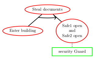
(a) A countermeasure from the Company.

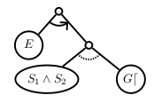
(b) Formal representation of the adt

Figure 1: Adts for the thief and company problem.

As said, the graphical model of Figure 1(a) is informal and cannot be exploited by any automated tool for reasoning. With the setting proposed in this contribution, we make it formal, and in particular we work out a new binary operator co for “countermeasure”, graphically reflected with a curved dashed line between two siblings: the left sibling is a proponent’s goal while the right sibling is the opponent’s countermeasure – with this convention, we can unambiguously retrieve the player’s type of an adt node. The more formal version of the adt in Figure 1(a) is drawn in Figure 1(b) (details for its construction can be found in Example 4).

The proposed semantics for adts also allows us to consider nested co operators to express countermeasures of countermeasures. For example, a proponent countermeasure against the company countermeasure could be to be disguised as an employee working in the building; we formalise this situation in Example 4. It should be observed that nested countermeasure is a core aspect of our contribution and the main subject of Section 5.

3 Attack-Defense Trees and Countermeasure-Depth

Preliminary notations

For the rest of this paper, we fix ${Prop}$ a finite set of propositions and we assume that the reader is familiar with propositional logic. We use typical symbol $\gamma$ for propositional formulas over ${Prop}$ and write a valuation of the propositional variables $a$ as an element of $\Sigma:=2^{{Prop}}$, that will be viewed as an alphabet. A trace $t$ over ${Prop}$, is finite word over $\Sigma$, that is a finite sequence of valuations. We denote the empty trace by $\varepsilon$, and we define $\Sigma^{+}:=\Sigma^{*}\backslash\{\varepsilon\}$. For a trace $t=a_{\_}1...a_{\_}n$, we define $|t|:=n$, its the length, as the number of valuations appearing in $t$, and we let $t[i]:=a_{\_}i$, for each $i\in\{1,\ldots,n\}$. We define the classic concatenation of traces: given two traces $t=a_{\_}1...a_{\_}n$ and $t^{\prime}=a_{\_}1^{\prime}...a^{\prime}_{\_}m$, we define $t\cdot t^{\prime}:=a_{\_}1...a_{\_}na_{\_}1^{\prime}...a_{\_}m^{\prime}$. We also lift this operator to sets of traces in the usual way: given two sets of traces $L$ and $L^{\prime}\subseteq\Sigma^{*}$, we let $L\cdot L^{\prime}:=\{t\cdot t^{\prime}~{}:~{}t\in L\text{ and }t^{\prime}\in L^{\prime}\}$. For a trace $t=a_{\_}1...a_{\_}n\in\Sigma^{*}$ and $1\leq i\leq n$, the trace $t^{\prime}=a_{\_}1...a_{\_}i$ is a prefix of $t$, written $t^{\prime}\preceq t$.

We define attack-defense trees (adts) over ${Prop}$, as well as their trace semantics and their countermeasure-depth, and develop enlightening examples. Adts are standard labeled finite trees with a dedicated set of labels based on the special $\epsilon$ label and propositional formulas for leaves and on the set $\{\texttt{\sc or},\texttt{\sc sand},\texttt{\sc and},\texttt{\sc co}\}$ for internal nodes.

Definition 1

The set ADT of adts over ${Prop}$ is inductively defined by:

• the empty-word leaf $\epsilon$ and every propositional formula $\gamma$ over ${Prop}$ are in ADT;

• if trees $\tau_{\_}1,...,\tau_{\_}n$ are in $ADT$, so are $\texttt{\sc or}(\tau_{\_}1,...,\tau_{\_}n)$, $\texttt{\sc sand}(\tau_{\_}1,...,\tau_{\_}n)$, and $\texttt{\sc and}(\tau_{\_}1,...,\tau_{\_}n)$;

• if trees $\tau$ and $\tau^{\prime}$ are in $ADT$, so is $\texttt{\sc co}(\tau,\tau^{\prime})$.

The size of an adt $\tau$, written $|\tau|$ is defined as the sum of the sizes of its leaves, provided the size of $\epsilon$ is $1$, while the size of $\gamma$ is its size when seen as a propositional formula.

Regarding the semantics, adts describe a set of traces over alphabet $\Sigma:=2^{Prop}$, hence their trace semantics. Formally, for an adt $\tau$, we define the language $Traces(\tau)\subseteq\Sigma^{*}$. First, we set $Traces(\epsilon)=\{\epsilon\}$. Now, a leaf adt hosting formula $\gamma$ denotes the reachability goal $\gamma$, that is the set of traces ending in a valuation satisfying $\gamma$ (we use the classic notations $\top=p\lor\lnot p$ and $\bot=\lnot\top$ with $p\in{Prop}$). We make our trace semantics compositional by providing the semantics of the four operators or, sand, co, and and in terms of how the subgoals described by their arguments interact. Operator or tells that at least one of the subgoals has to be achieved. Operator sand requires that all the subgoals need being achieved in the left-to-right order. The binary operator co requires to achieve the first subgoal without achieving the second one. Finally, operator and tells that all subgoals need to be achieved, regardless of the order. Without any countermeasure, and can be seen as a relaxation of the sand, but it is not true in general (see example 3).

At the level of the property described by an adt, i.e. a trace language, the operators correspond to specific language operations: or corresponds to union, sand to concatenation, co to a relativized complementation. Only and corresponds to a less classic operation: a trace $t$ belongs to the language of $\texttt{\sc and}(\tau_{\_}1,\tau_{\_}2)$ if $t$ belongs to the language of $\tau_{\_}1$ and has a prefix in the language of $\tau_{\_}2$ or vice-versa. Formally:

Definition 2

Let $L_{\_}1$, $L_{\_}2$ be two languages over alphabet $\Sigma$. The each of $L_{\_}1$ and $L_{\_}2$ is the language $L_{\_}1\sqcap L_{\_}2:=(L_{\_}1\cdot\Sigma^{*}\cap L_{\_}2)\cup(L_{\_}2\cdot\Sigma^{*}\cap L_{\_}1)$.

Because operator $\sqcap$ is associative, we can define $L_{\_}1\sqcap L_{\_}2\sqcap\ldots\sqcap L_{\_}n$ that amounts to being equal to $\bigcup_{\_}{i\in\{1,\ldots,n\}}(L_{\_}i\cap\bigcap_{\_}{j\neq i}L_{\_}j\cdot\Sigma^{*})$.

Example 1

A word $w=a_{\_}1a_{\_}2\ldots a_{\_}m$ belongs to $L_{\_}1\sqcap L_{\_}2\sqcap L_{\_}3$ whenever there are three (possibly equal) positions $i_{\_}1,i_{\_}2,i_{\_}3=m$ such that, for each $j\in\{1,2,3\}$, the word prefix $a_{\_}1\ldots a_{\_}{i_{\_}j}\in L_{\_}{\pi(j)}$, for some permutation $\pi$ of $(1,2,3)$.

We can now formally define the adt semantics.

Definition 3

• $Traces(\epsilon):=\{\varepsilon\}$ and $Traces(\gamma):=\{a_{\_}1...a_{\_}n\in\Sigma^{*}:a_{\_}n\models\gamma\}$;
  In particular, $Traces(\top)=\Sigma^{+}$ and $Traces(\bot)=\emptyset$;

• $Traces(\texttt{\sc or}(\tau_{\_}1,...,\tau_{\_}n)):=Traces(\tau_{\_}1)\cup...\cup Traces(\tau_{\_}n)$;

• $Traces(\texttt{\sc sand}(\tau_{\_}1,...,\tau_{\_}n)):=Traces(\tau_{\_}1)\cdot...\cdot Traces(\tau_{\_}n)$;

• $Traces(\texttt{\sc co}(\tau_{\_}1,\tau_{\_}2)):=Traces(\tau_{\_}1)\setminus Traces(\tau_{\_}2)$;

• $Traces(\texttt{\sc and}(\tau_{\_}1,...,\tau_{\_}n))=Traces(\tau_{\_}1)\sqcap...\sqcap Traces(\tau_{\_}n)$.

In the rest of the paper, we say for short that an adt is non-empty, written $\tau\neq\emptyset$, whenever $Traces(\tau)\neq\emptyset$. We say that two adts $\tau$ and $\tau^{\prime}$ are equivalent, whenever $Traces(\tau)=Traces(\tau^{\prime})$.

Remark 1

Since all operators $\cup$, $\cdot$ and $\sqcap$ over trace languages are associative, the trees of the form $\texttt{OP}(\tau_{\_}1,\texttt{OP}(\tau_{\_}2,\tau_{\_}3))$, $\texttt{OP}(\texttt{OP}(\tau_{\_}1,\tau_{\_}2),\tau_{\_}3)$, and $\texttt{OP}(\tau_{\_}1,\tau_{\_}2,\tau_{\_}3)$ are all equivalent, when OP ranges over $\{\texttt{\sc or},\texttt{\sc sand},\texttt{\sc and}\}$. As a consequence, we may sometime assume that nodes with such operators are binary.

We now introduce some notations for particular adts to ease our exposition and provide some examples of adts with their corresponding trace property.

We define a family of adts of the form $|{\geq\!\ell}|,|{<\!\ell}|,|{=\!\ell}|$, where $\ell$ is a non-zero natural. We let $|{\geq\!\ell}|:=\texttt{\sc sand}(\top,...,\top)$ where $\top$ occurs $\ell$ times; $|{<\!\ell}|:=\texttt{\sc co}(\top,|{\geq\!\ell}|)$; and $|{=\!\ell}|:=\texttt{\sc co}(|{\geq\!\ell}|,|{\geq\!\ell+1}|)$. It is easy to establish that adt $|{\geq\!\ell}|$ (resp. $|{<\!\ell}|$, $|{=\!\ell}|$) denotes the set of traces of length at least (resp. at most, exactly) $\ell$. We also consider particular adts and constructs for them.

• $\text{\sc all}:=\texttt{\sc or}(\epsilon,\top)$,

• $\text{\sc not}(\tau):=\texttt{\sc co}(\text{\sc all},\tau)$, and $\text{\sc inter}(\tau_{\_}1,\tau_{\_}2):=\text{\sc not}(\texttt{\sc or}(\text{\sc not}(\tau_{\_}1),\text{\sc not}(\tau_{\_}2)))$,

• $\rceil\tau\lceil:=\texttt{\sc sand}(\text{\sc all},\tau,\text{\sc all})$, $\rceil\tau:=\texttt{\sc sand}(\text{\sc all},\tau)$ and $\tau\lceil:=\texttt{\sc sand}(\tau,\text{\sc all})$.

• Given a formula $\gamma$ over ${Prop}$, we let $\underline{\gamma}:=\texttt{\sc co}(\gamma,|{\geq\!2}|)$.

Based on these notations, we develop further examples.

Example 2

• $Traces(\text{\sc all})=\Sigma^{*}$;

• $Traces(\text{\sc not}(\tau))=\Sigma^{*}\setminus Traces(\tau)$;

• $Traces(\text{\sc inter}(\tau_{\_}1,\tau_{\_}2))=Traces(\tau_{\_}1)\cap Traces(\tau_{\_}2)$;

• $Traces(\underline{\gamma})$ is set of one-length traces whose unique valuation satisfies $\gamma$; in particular, when a valuation $a$ is understood as a formula, namely formula $\bigwedge_{\_}{p\in a}p\land\bigwedge_{\_}{p\not\in a}\lnot p$, the adt $\underline{a}:=\texttt{\sc co}(a,|{\geq\!2}|)$ is such that $Traces(\underline{a})=\{a\}$;

• For a valuation $a$,

  • $Traces(\rceil\underline{a}\lceil)=Traces(\rceil a\lceil)=Traces(a\lceil)=\Sigma^{*}a\Sigma^{*}$;

  • $Traces(\rceil\underline{a})=Traces(\rceil a)=Traces(a)=\Sigma^{*}a$;

  • also, $Traces(\underline{a}\lceil)=a\Sigma^{*}$.

Example 3

Note that and cannot be seen as a kind of relaxation of sand. For the set of propositions $\{p\}$, if we consider the formula $p$ as a leaf, $Traces(\underline{p})=\{p\}$ and $Traces(\underline{\lnot p})=\{\emptyset\}$. Thus $\texttt{\sc sand}(\underline{\lnot p},\underline{p})=\{t\}$ with trace $t=\emptyset p$. However $\texttt{\sc and}(\underline{\lnot p},\underline{p})=\emptyset$. Let us notice that the construction of this example uses the co operator (hidden in $\underline{p}$ and $\underline{\neg p}$).

Example 4

We come back to the situation of our introductory example (Section 2). First, we discuss the formal semantics of the informal tree in fig. 1(a). To do so, we propose the following set of propositions: ${Prop}=\{E,S_{\_}1,S_{\_}2,G\}$ where $E$ holds when the thief is entering the building, $S_{\_}1$ (resp. $S_{\_}2$) holds when the first (resp. second) safe is open, and $G$ is true if a guard is in the building. The situation can be described by the following adt: $\tau_{\_}{ex_{\_}1}=\texttt{\sc sand}(E,\texttt{\sc co}(S_{\_}1\land S_{\_}2,G\lceil))$, represented in Figure 1(b), where we distinguish sand with a curved line and co with a dashed line. We have $Traces(\tau_{\_}{ex_{\_}1})=\{a_{\_}1...a_{\_}n\in\Sigma^{*}~{}:~{}a_{\_}n\models E\}\cdot\big{(}\{a_{\_}1...a_{\_}n\in\Sigma^{*}~{}:~{}a_{\_}n\models S_{\_}1\land S_{\_}2\}\setminus\{a_{\_}1...a_{\_}n\in\Sigma^{*}~{}:~{}\exists i$ such that $a_{\_}i\models G\}\big{)}$. If we write $\gamma_{\_}\varphi=\{a\in 2^{Prop}:a\models\varphi\}$, we have $Traces(\tau_{\_}{ex_{\_}1})=\Sigma^{*}\gamma_{\_}E\cdot(\Sigma^{*}\gamma_{\_}{S_{\_}1\wedge S_{\_}2}\setminus\Sigma^{*}\gamma_{\_}G\Sigma^{*})$. In other words, we want all traces where $E$ holds at some point and, after it, $G$ cannot be true and finish by a valuation where $S_{\_}1\land S_{\_}2$ holds.

In order to illustrate the nesting of countermeasures, we now allow the thief to disguise himself as an employee (assuming that when disguised, the guard does not identify him as a thief). To do so, we extended the set of propositions: ${Prop}^{\prime}=\{E,S_{\_}1,S_{\_}2,G,D\}$, where $D$ holds when the thief is disguised. The situation is now described by the following adt: $\tau_{\_}{ex_{\_}2}=\texttt{\sc sand}(E,\texttt{\sc co}(S_{\_}1\land S_{\_}2,\rceil\texttt{\sc co}(G,D)\lceil))$. The semantics for $\tau_{\_}{ex_{\_}2}$ is all traces where $E$ holds at some point and, after it, $G$ cannot be true, except if $D$ holds at the same time, and finish by a valuation where $S_{\_}1\land S_{\_}2$ holds. A representation of $\tau_{\_}{ex_{\_}2}$ can be found in Appendix 0.A

We now stratify the set ADT of adts according to their countermeasure-depth that denotes the maximum number of nested countermeasures.

Definition 4

The countermeasure-depth of an adt $\tau$, written $\delta(\tau)$, is inductively defined by:

• $\delta(\epsilon):=\delta(\gamma)=0$;

• $\delta(\texttt{OP}(\tau_{\_}1,...,\tau_{\_}n)):=\max\{\delta(\tau_{\_}1),...,\delta(\tau_{\_}n)\}$ for every $\texttt{OP}\in\{\texttt{\sc or},\texttt{\sc sand},\texttt{\sc and}\}$;

• $\delta(\texttt{\sc co}(\tau_{\_}1,\tau_{\_}2)):=\max\{\delta(\tau_{\_}1),\delta(\tau_{\_}2)+1\}$

We let ${ADT}_{k}:=\{\tau\in ADT~{}:~{}\delta(\tau)\leq k\}$ be the set of adts with countermeasure-depth at most $k$. Clearly ${ADT}_{0}\subseteq{ADT}_{1}\subseteq\ldots{ADT}_{k}\subseteq{ADT}_{k+1}\subseteq\ldots$, and $ADT=\underset{k\in\mathbb{N}}{\bigcup}{ADT}_{k}$.

Example 5

We list a couple of examples. $\delta(\text{\sc not}(\tau))=1+\delta(\tau)$; $\delta(\text{\sc inter}(\tau_{\_}1,\tau_{\_}2))=2+\max\{\delta(\tau_{\_}1),\delta(\tau_{\_}2)\}$; $\delta(\texttt{\sc co}(\texttt{\sc co}(\gamma_{\_}1,\gamma_{\_}2),\gamma_{\_}3))=1$ while $\delta(\texttt{\sc co}(\gamma_{\_}3,\texttt{\sc co}(\gamma_{\_}2,\gamma_{\_}3)))=2$; $\delta(|{<\!\ell}|)=\delta(|{=\!\ell}|)=1$ while $\delta(|{\geq\!\ell}|)=0$; $\delta(\underline{\gamma})=1$; In Example 4, $\delta(\tau_{\_}{ex_{\_}1})=1$ and $\delta(\tau_{\_}{ex_{\_}2})=2$.

Also, $\delta(|{\geq\!\ell}|)=0$, $\delta(|{<\!\ell}|)=\delta(|{=\!\ell}|)=1$, so that $|{\geq\!\ell}|\in{ADT}_{0}$; $|{<\!\ell}|$ and $|{=\!\ell}|\in{ADT}_{1}$. Moreover, $\tau_{\_}{ex_{\_}1}\in{ADT}_{1}$ and $\tau_{\_}{ex_{\_}2}\in{ADT}_{2}$.

We say that a language $L$ is ${ADT}_{k}$-definable (resp. $ADT$-definable), written $L\in{ADT}_{k}$ (resp. $ADT$), whenever $Traces(\tau)=L$, for some $\tau\in{ADT}_{k}$ (resp. for some $k$).

It can be established that non-empty adts in ${ADT}_{1}$ enjoy small traces, i.e. smaller than the size of the tree.

Theorem 3.1 (Small model property for ${ADT}_{1}$)

An adt $\tau\in{ADT}_{1}$ is non-empty if, and only if, there is a trace $t\in Traces(\tau)$ with $|t|\leq|\tau|$.

We here only sketch the proof, whose details can be found in Appendix 0.B. The technique we employ consists in defining a slight variant of the classic relation of super-word in language theory, that we call the lift binary relation. We prove that if $\tau\in{ADT}_{1}$, then there exists a finite set of generators, denoted $gen(\tau)$, which is sufficient to describe $Traces(\tau)$ through the lift relation. Next, we can prove that the traces in $gen(\tau)$ have size bounded by the number of leaves of $\tau$. Notice that the result also holds for ${ADT}_{0}$, since ${ADT}_{0}\subseteq{ADT}_{1}$.

4 Adts, Star-free Languages, and First-Order Logic

We prove that adts coincide with star-free languages and first order formulas.

4.1 Reminders on Star-free Languages and First-Order Logic

The class of star-free languages introduced by [11, 4, 15] (over alphabet $\Sigma$) is obtained from the finite languages (or alternatively languages consisting of a single one-length word in $\Sigma$) by finitely many applications of Boolean operations ($\cup$, $\cap$ and $\sim$ for the complement) and the concatenation product (see [18, Chapter 7]). Alternatively, one characterizes star-free languages by first considering extended regular expressions – that are regular expressions augmented with intersection and complementation, and second by restricting to star-free extended regular expressions (SEREs, for short) that are extended regular expressions with no Kleene-star operator. Regarding computational complexity aspects, we recall the following the subclass of SEREs of extended regular expressions. The word membership problem (i.e., whether a given word belongs to the language denoted by a SERE) is in Ptime [9, Theorem 2], while the non-emptiness problem (i.e., is the denoted language empty?) and the equivalence problem (i.e., do two SEREs denote the same language?) are hard, both non-elementary [21, p. 162].

We now recall classical results on the first-order logic on finite words FO$[<]$ (see details in [14, Chapter 29]). The signature of FO$[<]$, say for words over an alphabet $\Sigma$, is composed of a unary predicate $a(x)$ for each $a\in\Sigma$, whose meaning is the “letter at position $x$ of the word is $a$”, and the binary predicate $x<y$ that states “position $x$ is strictly before position $y$ in the word”. For a FO$[<]$-formula, we define its size $|\psi|$ as the size of the expression considered as a word. A language $L$ is FO$[<]$-definable whenever there exists a FO$[<]$-formula $\psi$ such that a word $w\in L$ if, and only if, $w$ is a model of $\psi$. Similarly, we say that an adt $\tau$ is FO$[<]$-definable if $Traces(\tau)$ is FO$[<]$-definable. It is well-known that FO$[<]$-definable languages coincide with star-free languages [11, 22, 13].

Also, for a fine-grained inspection of FO$[<]$, let us denote by $\Sigma_{\ell}$ (resp. $\Pi_{\ell}$) the fragments of FO$[<]$ consisting of formulas with at most $\ell$ alternation of $\exists$ and $\forall$ quantifier blocks, starting with $\exists$ (resp. $\forall$). The folklore results regarding satisfiability of FO$[<]$-formulas [21, 12] are: (a) The satisfiability problem for FO$[<]$ is non-elementary; (b) The satisfiability for $\Sigma_{\ell}$ is in $(\ell-1)$-Expspace . We are not aware of any result that establishes a tight lower bound complexity for the satisfiability problem on the $\Sigma_{\ell}$ fragments of FO$[<]$.

We lastly recall the definition of the dot-depth hierarchy of star-free languages: level $0$ of this hierarchy is $B_{0}:=\{L\subseteq 2^{\Sigma}:L$ is finite or co-finite}, and evel $\ell$ is $B_{\ell}:=\{L\subseteq 2^{\Sigma}:L$ is a Boolean combination of languages of the form $L_{\_}1\cdot...\cdot L_{\_}n$ where $L_{\_}1,...,L_{\_}n\in B_{\ell-1}\}$. The dot-depth hierarchy has a tight connection with FO$[<]$ fragments [22]: for every $\ell>0$, $\Sigma_{\ell}\subseteq B_{\ell}\subseteq\Sigma_{\ell+1}$.

4.2 Expressiveness of Adts

The first result of this section consist in showing that adts and star-free extended regular expressions share the same expressiveness.

Theorem 4.1

A language $L$ is star-free if, and only if, $L$ is $ADT$-definable.

For the “only if” direction of Theorem 4.1, we reason by induction on the class of star-free languages. For a language of the form $\{a\}$ where $a\in\Sigma$ one can take the adt $\underline{a}$ (that is $\texttt{\sc co}(a,|{\geq\!2}|)$). Now we can inductively build adequate adts for compound star-free languages by noticing that language operations of union and concatenation are captured by adts operators or and sand respectively, while complementation and intersection are obtained from the $\text{\sc not}(.)$ and $\text{\sc inter}(.,.)$ as formalized in Example 2. One easily verifies that that the size of the adt corresponding to an SERE $E$ is in $O(|E|)$, where $|E|$ denotes the size (number of characters) of $E$.

For the “if” direction of Theorem 4.1, it is easy to translate an adt into an SERE: the leaf $\epsilon$ translates into $\epsilon$, a leaf adt $\gamma$ translates into $\bigcup_{\_}{a\models\gamma}a$ – notice that this translation is exponential. For non-leaf adts, since every operator occurring in the adt has its language-theoretic counterpart the translation goes smoothly. However, the translation is exponential because of the adt operator and, see Definition 2.

We now dig into the ADT-hierarchy induced by the countermeasure-depth and compare it with the FO$[<]$ fragments $\Sigma_{\ell}$ and $\Pi_{\ell}$.

We first step design a translation from ADT into FO$[<]$, inductively over adts. The translation of an adt $\tau$ is written $\psi_{\_}\tau$. For the base cases of adts $\epsilon$ and $\gamma$, and we let: $\psi_{\_}\epsilon:=\forall x\bot$ and $\psi_{\_}\gamma:=\exists x(\forall y\lnot(x<y)\land\bigvee_{\_}{a\models\gamma}a(x))$.

Now, regarding compound adts, and not surprisingly, operator or is reflected by the logical disjunction: $\psi_{\_}{\texttt{\sc or}(\tau_{\_}1,\tau_{\_}2)}:=\psi_{\_}{\tau_{\_}1}\lor\psi_{\_}{\tau_{\_}2}$, while operator co is reflected by means of the logical conjunction with the negated second argument: $\psi_{\_}{\texttt{\sc co}(\tau_{\_}1,\tau_{\_}2)}:=\psi_{\_}{\tau_{\_}1}\land\lnot\psi_{\_}{\tau_{\_}2}$. On the contrary, the two remaining operators sand and and require to split the trace into pieces, which can be captured by the folklore operation of left (resp. right) position relativizations of FO$[<]$-formulas w.r.t. a position [13, Proposition 2.1] (see also formulas of the form $\phi^{[x,y]}$ in [19]). Formally, given a position $x$ in the trace $t$ and an FO$[<]$-formula $\psi$, we define formula ${\psi}^{\leq x}$ (resp. ${\psi}^{>x}$) that holds of $t$ if the prefix (resp. suffix) of $t$ up to (resp. from) position $x$ satisfies $\psi$, as follows. For ${\bowtie}\in\{\leq,>\}$, we let:

${a(y)}^{\bowtie x}=a(y)$

${(y<z)}^{\bowtie x}=(y<z)$

${p(y)}^{\bowtie x}=p(y)$

${(\psi\lor\psi^{\prime})}^{\bowtie x}={\psi}^{\bowtie x}\lor{\psi^{\prime}}^{\bowtie x}$

${(\lnot\psi)}^{\bowtie x}=\lnot{\psi}^{\bowtie x}$

${(\exists y\,\psi)}^{\bowtie x}=\exists y~{}(y\bowtie x\land{\psi}^{\bowtie x})$

Additionally, we write ${\psi}^{\leq 0}$ and ${\psi}^{>0}$ as the formulas obtained from ${\psi}^{\leq x}$ and ${\psi}^{>x}$ by replacing every occurrence of expressions $y\leq x$ and $y>x$ by $\bot$ and $\top$ respectively.

Remark 2

For every formula $\psi\in\Sigma_{\ell}$, we also have ${\psi}^{\leq x},{\psi}^{>x}\in\Sigma_{\ell}$.

We can now complete the translation from ADT into FO$[<]$ by letting (w.l.o.g., by Remark 1, we can consider binary sand and and):

$\psi_{\_}{\texttt{\sc sand}(\tau_{\_}1,\tau_{\_}2)}:=\exists x[{\psi_{\_}{\tau_{\_}1}}^{\leq x}\land{\psi_{\_}{\tau_{\_}2}}^{>x}]\lor({\psi_{\_}{\tau_{\_}1}}^{\leq 0}\land\psi_{\_}{\tau_{\_}2})$

$\psi_{\_}{\texttt{\sc and}(\tau_{\_}1,\tau_{\_}2)}:=\exists x[({\psi_{\_}{\tau_{\_}1}}^{\leq x}\land\psi_{\_}{\tau_{\_}2})\lor({\psi_{\_}{\tau_{\_}2}}^{\leq x}\land\psi_{\_}{\tau_{\_}1})]\lor({\psi_{\_}{\tau_{\_}1}}^{\leq 0}\land\psi_{\_}{\tau_{\_}2})\lor({\psi_{\_}{\tau_{\_}2}}^{\leq 0}\land\psi_{\_}{\tau_{\_}1})$.

Lemma 1 ()

• For any $t\in\Sigma^{*}$, $t\models\psi_{\_}{\tau}$ iff $t\in Traces(\tau)$.

• For any adt $\tau$, formula $\psi_{\_}{\tau}$ is of size exponential in $|\tau|$.

In the rest of the paper, we use mere inclusion symbol $\subseteq$ between subclasses of ADT and subclasses of FO$[<]$, with the canonical meaning regarding the denoted trace languages.

An accurate inspection of the translation $\tau\mapsto\psi_{\_}\tau$ entails that every ${ADT}_{k}$-definable adt can be equivalently represented by a $\Sigma_{k+2}$-formula, namely ${ADT}_{k}\subseteq\Sigma_{k+2}$. However, we significantly refine this expressiveness upperbound for ${ADT}_{k}$.

Lemma 2 ()

1. ${ADT}_{0}\subseteq\Sigma_{2}\cap\Pi_{2}$ – with an effective translation.

2. For every $k>0$, ${ADT}_{k}\subseteq\Sigma_{k+1}$ – with an effective translation.

Regarding Item 1 of Lemma 2, it can be observed that, whenever $\tau\in{ADT}_{0}$, the quantifiers $\forall$ and $\exists$ commute in $\psi_{\_}\tau$ (see Appendix 0.C). Now, for Item 2, the proof is conducted by induction over $k$ (see Remark 4). We sketch here the case $k>1$. First, remark that if $\tau_{\_}1,...,\tau_{\_}n\in{ADT}_{k-1}$ are $\Sigma_{k}$-definable, then $\texttt{\sc or}(\tau_{\_}1,...,\tau_{\_}n),\texttt{\sc sand}(\tau_{\_}1,...,\tau_{\_}n)$ and $\texttt{\sc and}(\tau_{\_}1,...,\tau_{\_}n)$ remain $\Sigma_{k}$-definable, as formulas are obtained from conjunctions or disjunctions of $\Sigma_{k}$-definable formulas. Moreover, if $\tau_{\_}1$ and $\tau_{\_}2$ are $\Sigma_{k}$-definable, then $\tau=\texttt{\sc co}(\tau_{\_}1,\tau_{\_}2)$ is $\Sigma_{k+1}$-definable as a formula can be obtained from a boolan combination of two $\Sigma_{k}$-definable formulas. Finally, with $k$ still fixed, it can be shown by induction over the size of an adt $\tau$ that, if $\tau\in{ADT}_{k}$, since all its countermeasures operators are of the form $\texttt{\sc co}(\tau_{\_}1,\tau_{\_}2)$ where $\tau_{\_}1\in{ADT}_{k}$ and $\tau_{\_}2\in{ADT}_{k-1}$, we have that adt $\tau$ is also $\Sigma_{k+1}$-definable, which concludes.

We can also establish lowerbounds in the ADT-hierarchy.

Lemma 3 ()

1. $B_{\ell}\subseteq{ADT}_{2\ell+2}$, and therefore $\Sigma_{\ell}\subseteq{ADT}_{2\ell+2}$

2. $\Sigma_{1}\subseteq{ADT}_{0}$ – with an effective translation.

Item 1 of Lemma 3 is obtained by an induction of $\ell$. Regarding Item 2, the translation consists in putting the main quantifier-free subformula of a $\Sigma_{1}$-formula in disjunctive normal form, and to focus for each conjunct on the set of "ordering" literals of the form $x<y$ or $\lnot(x<y)$ (leaving aside the other literals of the form $a(x)$ or $\lnot a(x)$ for a while). Each ordering literal naturally induces a partial order between the variables. We expend this partial order constraint over the variables as a disjunction of all its possible linearizations. For example, the conjunct $x<y\land\lnot(y<z)$ is expended as the equivalent formula $(x<y\land y=z)\lor(x<z\land z<y)\lor(z=x\land x<y)\lor(z<x\land x<y)$. Now, each disjunct of this new formula, together with the constraints $a(x)$ (or $\lnot a(x)$), can easily be specified by a sand-rooted adt (ie. the root is a sand). The initial $\Sigma_{1}$-formula then is associated with the or-rooted tree that gathers all the aforementioned sand-rooted subtrees (see Remark 3 in Appendix 0.B). Notice that the translation may induce at least an exponential blow-up.

The reciprocal of Item 2 in Lemma 3 is an open question. Still, we have little hope that it holds because $\psi_{\_}{\gamma}$ seems to require a property expressible in $\Sigma_{2}\setminus\Sigma_{1}$.

5 Strictness of the ADT-Hierarchy

One can notice that the adt $|{<\!2}|\in{ADT}_{1}$ defines the finite language of traces of length at most $1$, while it can be established that languages arising from adts in ${ADT}_{0}$ are necessarily infinite – if inhabited by a non-empty word (see Lemma 4 of Appendix 0.B). Thus, we can easily deduce ${ADT}_{0}\subsetneq{ADT}_{1}$. This section aims at showing that the entire ADT-hierarchy is strict:

Proposition 1

For every $k\in\mathbb{N}$, ${ADT}_{k}\subsetneq{ADT}_{k+1}$, even if ${Prop}=\{p\}$.

To show that ${ADT}_{k}\subsetneq{ADT}_{k+1}$, we use a family of languages, originally introduced in [23], that we write $\{{W_{k}}\}_{\_}{k\in\mathbb{N}}$ over the two-letter alphabet $\Sigma$ obtained from ${Prop}=\{p\}$. For readability, we use symbol $a$ (resp. $b$) for the valuation $\{p\}$ (resp. $\emptyset$) of $\Sigma$. Formally, we define ${W_{k}}\subseteq\Sigma^{*}$ as follows – where $\lVert w\rVert$ denotes the number of occurrences of $a$ minus the number of occurrences of $b$ in the word $w$:

We let $w\in{W_{k}}$ whenever all the following holds.

• $\lVert w\rVert=0$;

• for every $w^{\prime}\preceq w$, $0\leq\lVert w^{\prime}\rVert\leq k$;

• there exists $w^{\prime\prime}\preceq w$ s.t. $\lVert w^{\prime\prime}\rVert=k$.

In [23, Theorem 2.1], it is shown that ${W_{k}}\in B_{k}\setminus B_{k-1}$, for all $k\geq 1$.

We now determine the position of ${W_{k}}$ languages in the ADT-hierarchy. We show Proposition 2.

Proposition 2 ()

For each $k>0$, ${W_{k}}\in{ADT}_{k+1}\setminus{ADT}_{k-2}$.

First, ${W_{k}}\notin{ADT}_{k-2}$ because ${W_{k}}$ is not $\Sigma_{k-1}$-definable ([23]). By an inductive argument over $k$ (see Appendix 0.D), we can build an adt $\mu_{k}\in{ADT}_{k+1}$ that captures ${W_{k}}$. We only sketch here the case $k=1$. For ${W_{1}}$, we set $\mu_{1}:=\texttt{\sc co}(b,\texttt{\sc or}(\underline{b}\lceil,\rceil\texttt{\sc co}(|{\geq\!2}|,\texttt{\sc and}(a\lceil,b\lceil))\lceil))$, depicted in Figure 2(a). Note that $\delta(\mu_{1})=2$ and that by a basic use of semantics, we have $Traces(\mu_{1})=(ab)^{+}={W_{1}}$.

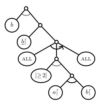
(a) Representation of $\mu_{1}$

(b) Summary of the results on ADT-hierarchy

Now we have all the material to prove Proposition 1. Indeed, assuming the hierarchy collapses at some level will contradict Proposition 2. Notice that this argument is not constructive as we have no witness of ${ADT}_{k}\subsetneq{ADT}_{k+1}$ but for $k=1$ where it can be shown that $(ab)^{+}\in{ADT}_{2}\setminus{ADT}_{1}$ (see Appendix 0.B, Example 7 and Proposition 3). Our results about the ADT-hierarchy are depicted on Figure 2(b).

6 Decision Problems on Attack-Defense Trees

We study classical decision problems on languages, through the lens of adts, with a focus on the role played by the countermeasure-depth in their complexities. The problems are the following.

• The membership problem, written ${ADT}$-memb, is defined by:
  Input: $\tau$ an attack-defense tree and $t$ a trace. Output: "YES" if $t\in Traces(\tau)$, "NO" otherwise.

• The non-emptiness problem, written ${ADT}$-ne, is defined by:
  Input: $\tau$ an attack-defense tree. Output: "YES" if $Traces(\tau)\neq\emptyset$, "NO" otherwise.

We use notations ${ADT}_{k}$-memb and ${ADT}_{k}$-ne whenever the input adts of the respective decision problems are in ${ADT}_{k}$, with a fixed $k$. Our results are summarized in Table 1, and we below comment on them, row by row.

[b] ${ADT}_{0}$ ${ADT}_{1}$ ${ADT}_{k}$ $(k\geq 2)$ $ADT$ ${ADT}$-memb Ptime Ptime Ptime Ptime ${ADT}$-ne NP -comp NP -comp $(k+1)$-Expspace non-elem ¹  $\geq$ $\mbox{\sc Nspace}(g(k-5,c\sqrt{\frac{n-1}{3}}))$ ${ADT}$-equiv coNP -comp $4$-Expspace $(k+2)$-Expspace non-elem ²  $\geq$ $\mbox{\sc Nspace}(g(k-4,c\sqrt{\frac{n-1}{3}}))$

• if $k\geq 5$.

• if $k\geq 4$.

Table 1: Computational complexities of decision problems on adts.

Regarding ${ADT}$-memb (first row of Table 1), we recall that adts and SEREs are expressively equivalent, but with a translation (Theorem 4.1) from the former to the latter that is not polynomial. We therefore cannot exploit [9, Theorem 2] for a Ptime complexity of the word membership problem for SEREs, and have instead developed a dedicated alternating logarithmic-space algorithm in Appendix 0.E.

Regarding ${ADT}$-ne (second row of Table 1), and because SEREs can be translated as adts (see “if” direction in the proof of Theorem 4.1), the problem ${ADT}$-ne inherits from the hardness of the non-emptiness of SEREs [21, p. 162]. In its full generality, ${ADT}$-ne is therefore non-elementary (last column). Moreover, by our exponential translation of ${ADT}_{k}$ into the FO$[<]$-fragment $\Sigma_{k+1}$ (Lemma 2), we obtain the $(k+1)$-Expspace upper-bound complexity for ${ADT}_{k}$-ne (recall satisfiability problem for $\Sigma_{\ell}$ is $(\ell-1)$-Expspace ). Additionally, a lower-bound for ${ADT}_{k}$-ne is directly given by [21, Theorem 4.29]: for SEREs that linearly translate as adts with countermeasure-depth $k$, their non-emptiness is at least $\mbox{\sc Nspace}(g(k-5,c\sqrt{\frac{n-1}{3}}))$. Interestingly, the Small Model Property (Theorem 3.1) yields an NP upper-bound complexity for ${ADT}_{1}$-ne, also applicable for ${ADT}_{0}$-ne, that is optimal since one can reduce the NP -complete satisfiability of propositional formulas to the non-emptiness of leaf adts.

Finally regarding ${ADT}$-equiv (last row of Table 1), one can observe that ${ADT}$-ne and ${ADT}$-equiv are very close. First, ${ADT}$-ne is a particular case of ${ADT}$-equiv with the second input adt $\tau_{\_}2:=\emptyset$. As a consequence, ${ADT}$-equiv inherits from the hardness of ${ADT}$-ne, and is therefore non-elementary (last column). Also, because deciding the equivalence between $\tau_{\_}1$ and $\tau_{\_}2$ amounts to deciding whether $\texttt{\sc or}(\texttt{\sc co}(\tau_{\_}1,\tau_{\_}2),\texttt{\sc co}(\tau_{\_}2,\tau_{\_}1))=\emptyset$, we get reduction from ${ADT}_{k}$-equiv into ${ADT}_{k+1}$-ne which provides the results announced in Columns 1-3.

7 Discussion

First, we discuss our model of adts with regard to the literature. However, we do not compare with settings where adts leaves are actions [10], as they yield only finite languages, and address other issues [24].

Our adts have particular features, but remain somehow standard. Regarding the syntax, firstly, even though we did not type our nodes as proponent/opponent, the countermeasure operator fully determines the alternation between attack and defense. Also, we introduced the non-standard leaf $\epsilon$ for the singleton empty-trace language, not considered in the literature. Still, it is a very natural object in the formal language landscape, and anyhow does not impact our overall computational complexity analysis. Regarding the semantics, it can be shown that the definition of our operator and together with the reachability goal semantics of the leaves coincides with the acknowledged semantics considered in [1, 2].

Second, we discuss our results. We showed the strictness of the $ADT$-hierarchy in a non-constructive manner. However, exhibiting an element of ${ADT}_{k+1}\setminus{ADT}_{k}$ ($k\geq 2$) is still an open question. Since ${W_{1}}\in{ADT}_{2}\setminus{ADT}_{1}$, languages ${W_{k}}$ are natural candidates. We conjecture it is the case and we are currently working on Erenfeucht-Fraissé(EF)-like games for adts (in the spirit of [23] for SEREs) to prove it. Moreover, EF-like games for adts may also help to better compare the ADT-hierarchy and the FO$[<]$ alternation hierarchy, in particular, whether the hierarchies eventually coincide. For now, finding a tighter inclusion of $\Sigma_{\ell}$ in some ${ADT}_{k}$ for each $\ell$ seems difficult; recall that we established $\Sigma_{\ell}\subseteq{ADT}_{2\ell+2}$. Any progress in this line would be of great help to obtain tight complexity bounds for ${ADT}_{k}$-ne and ${ADT}_{k}$-equiv. Finally, determining the level of a language in the ADT-hierarchy seems as hard as determining its level in the dot-depth hierarchy, recognised as a difficult question [17, 3].

Appendix 0.A Figure of $\tau_{\_}{ex_{\_}2}$ in Example 4

Appendix 0.B Proof of Theorem 3.1

We consider the lift binary relation between traces (Definition 5), a slight variant of the classic relation of super-word in language theory. We use the lift to define generators of a set of traces (see Definition 6) for $\tau$ an adt. We define (in Definition 7) $gen(\tau)$, a finite set of traces, and we show in Proposition 3 that, if $\tau\in{ADT}_{1}$, then $gen(\tau)$ is a set of generators of the semantics of $\tau$. We also show in Lemma 5 that an element of $gen(\tau)$ has its size bounded by the number of leaves of $\tau$. Lemma 5 and Proposition 3 are enough to deduce the small model property of ${ADT}_{1}$, stated in Theorem 3.1.

Definition 5

A trace $t$ is a lift of a trace $t^{\prime}=a_{\_}1...a_{\_}n$, written $t^{\prime}\sqsubseteq t$, whenever $t\in\Sigma^{*}a_{\_}1...\Sigma^{*}a_{\_}n$.

Notice that $\sqsubseteq$ is an order over $\Sigma^{*}$ and that lift relation is like the relation of super-word where the last letters of the respective traces are identical. It can be shown by induction of trees that every $\tau\in{ADT}_{0}$, the set $Traces(\tau)$ is $\sqsubseteq$-upward closed, and is therefore infinite:

Lemma 4

Let $\tau\in{ADT}_{0}$. If $t\in Traces(\tau)$, then for each trace $t^{\prime}$ such that $t\sqsubseteq t^{\prime}$, we have $t^{\prime}\in Traces(\tau)$.

Proof

We show this result by induction over the shape of an adt.

If $\tau=\epsilon$, then there is no lift of $\varepsilon$. If $\tau$ is a non-empty leaf $\gamma$, the result holds since the lift relation preserves the last letter.

Now, we assume that the result holds for two adts $\tau_{\_}1$ and $\tau_{\_}2$ and we need to show the result for $\texttt{\sc or}(\tau_{\_}1,\tau_{\_}2)$, $\texttt{\sc sand}(\tau_{\_}1,\tau_{\_}2)$ and $\texttt{\sc and}(\tau_{\_}1,\tau_{\_}2)$.

The three cases are direct and similar, we only write the case $\tau=\texttt{\sc sand}(\tau_{\_}1,\tau_{\_}2)$: if $t\in Traces(\tau)$ and $t\sqsubseteq t^{\prime}$ for a certain trace $t^{\prime}$, then we can write $t=t_{\_}1\cdot t_{\_}2$ with $t_{\_}1\in Traces(\tau_{\_}1)$ and $t_{\_}2\in Traces(\tau_{\_}2)$. From the structure of a lift, we can also write $t^{\prime}=t^{\prime}_{\_}1\cdot t^{\prime}_{\_}2$ such that $t_{\_}1\sqsubseteq t^{\prime}_{\_}1$ and $t_{\_}2\sqsubseteq t^{\prime}_{\_}2$, we can then conclude with our induction hypothesis.

From Lemma 4, it is immediate that any non-empty semantics of an adt in ${ADT}_{0}$ is necessarily infinite. We now turn to the notion of generators to establish the Small Model Property.

Definition 6

Let $L\subseteq\Sigma^{*}$. A set of generators of $L$ is a finite subset $G$ of $L$ with the following property: for each non-empty trace $t_{\_}L\in L$ there exists $t_{\_}{gen}=a_{\_}1...a_{\_}n\in G$ such that we can write $t_{\_}L=w_{\_}1a_{\_}1...w_{\_}na_{\_}n$ and for each $t\in\Sigma^{*}$, if we can write $t=w_{\_}1^{\prime}a_{\_}1...w_{\_}1^{\prime}a_{\_}n$ with $w_{\_}1^{\prime}a_{\_}1\sqsubseteq w_{\_}1a_{\_}1$, …, $w_{\_}n^{\prime}a_{\_}n\sqsubseteq w_{\_}na_{\_}n$, then $t\in L$.

Example 6

For the singleton set of propositions $\{p\}$, we consider the set of traces $L=p^{+}\setminus\{pp\}$. The set $\{p,ppp\}$ is a set of generators for $T$. However, the set $\{p\}$ is not because we have $ppp\in T$ and $p\sqsubseteq ppp$ but we also have $p\sqsubseteq pp\sqsubseteq ppp$ and $pp\notin T$.

Example 7

For the singleton set of propositions $\{p\}$, we let $a$ be the valuation that makes $p$ true and $b$ the valuation that makes $p$ false. Thus each trace is a word over the alphabet $\{a,b\}$. Now, remark that the set $(ab)^{+}$ has no set of generators. Indeed, assume that $G\subseteq(ab)^{+}$ is a set of generators. We write $(ab)^{N}$ for the largest element of $G$, thus $(ab)^{N}ab\in(ab)^{+}\setminus G$. However, for each $t_{\_}{gen}\in G$, we have $t_{\_}{gen}\sqsubseteq(ab)^{N}b\sqsubseteq(ab)^{N}ab$ and $(ab)^{N}b\notin(ab)^{+}$, which contradicts Definition 6.

We now define the set $gen(\tau)$ for each adt $\tau$ that will be our candidate to show that every of adts in ${ADT}_{1}$ has a set of generators.

Definition 7

Let $\tau\in{ADT}_{1}$. The set $gen(\tau)$ is inductively defined as follows:

• $gen(\epsilon)=\emptyset$ and $gen(\gamma)=\{a\in 2^{Prop}:a\models\gamma\}$,

• $gen(\texttt{\sc or}(\tau_{\_}1,\tau_{\_}2))=gen(\tau_{\_}1)\cup gen(\tau_{\_}2)$,

• $gen(\texttt{\sc sand}(\tau_{\_}1,\tau_{\_}2))=gen(\tau_{\_}1)\cdot gen(\tau_{\_}2)$,

• $gen(\texttt{\sc co}(\tau_{\_}1,\tau_{\_}2))=gen(\tau_{\_}1)\setminus Traces(\tau_{\_}2)$,

• $gen(\texttt{\sc and}(\tau_{\_}1,\tau_{\_}2))=(gen(\tau_{\_}1)\bowtie gen(\tau_{\_}2))\cap Traces(\texttt{\sc and}(\tau_{\_}1,\tau_{\_}2))$, where $\bowtie$ is the classic shuffle operator inductively defined as: $\varepsilon\bowtie t=t\bowtie\varepsilon=\{t\}$, $a_{\_}1t_{\_}1\bowtie a_{\_}2t_{\_}2=a_{\_}1\cdot(t_{\_}1\bowtie a_{\_}2t_{\_}2)\cup a_{\_}2\cdot(a_{\_}1t_{\_}1\bowtie t_{\_}2)$ and $at_{\_}1\bowtie at_{\_}2=a\cdot(t_{\_}1\bowtie at_{\_}2)\cup a\cdot(at_{\_}1\bowtie t_{\_}2)\cup a\cdot(t_{\_}1\bowtie t_{\_}2)$.

We can prove the following Lemma 5 by induction over adts.

Lemma 5 ()

For each trace $t\in gen(\tau)$, its size $|t|$ is bounded by the number of leaves of $\tau$.

Proof

We show this result by induction over the shape of an adt.

If the adt is the empty leaf $\epsilon$, then there is no element in $gen(\tau)$. If adt is a non-empty leaf $\gamma$ then all elements of $gen(\tau)$ are of size 1.

Now, we assume that the result holds for two adts $\tau_{\_}1$ and $\tau_{\_}2$ and we show the result for $gen(\texttt{\sc or}(\tau_{\_}1,\tau_{\_}2))$, $gen(\texttt{\sc sand}(\tau_{\_}1,\tau_{\_}2))$, $gen(\texttt{\sc and}(\tau_{\_}1,\tau_{\_}2))$ and $gen(\texttt{\sc co}(\tau_{\_}1,\tau_{\_}2))$. For the rest of the proof, we write $n_{\_}1$ the number of leaves of $\tau_{\_}1$ and $n_{\_}2$ the number of leaves of $\tau_{\_}2$.

By induction, if $t\in gen(\texttt{\sc or}(\tau_{\_}1,\tau_{\_}2))$, then $|t|\leq MAX\{n_{\_}1,n_{\_}2\}$. If $t\in gen(\texttt{\sc sand}(\tau_{\_}1,\tau_{\_}2))$ or $t\in gen(\texttt{\sc and}(\tau_{\_}1,\tau_{\_}2))$, then $|t|\leq n_{\_}1+n_{\_}2$. Finally, if $t\in gen(\texttt{\sc co}(\tau_{\_}1,\tau_{\_}2))$, then $|t|\leq n_{\_}1$. In each case, $|t|\leq n_{\_}1+n_{\_}2$ and $n_{\_}1+n_{\_}2$ is the number of leaves of the four studied adts, which concludes.

If $\tau$ has no nested countermeasures yields the following.

Proposition 3 ()

When $\tau\in{ADT}_{1}$, the set $gen(\tau)$ is a set of generators for $Traces(\tau)$.

Proof

We show this result by induction over the shape of an adt.

If $\tau=\epsilon$, then its semantics contains only the empty trace. Thus $\emptyset$ is a set of generators. If $\tau=\gamma$, then $Traces(\gamma)=\{a_{\_}1...a_{\_}n\in\Sigma^{*}:a_{\_}n\models\gamma\}=\Sigma^{*}\cdot gen(\gamma)$, thus $gen(\gamma)\subseteq Traces(\gamma)$ and is a set of generators.

Now, for two adts $\tau_{\_}1$ and $\tau_{\_}2$, we assume that $gen(\tau_{\_}1)$ and $gen(\tau_{\_}2)$ are sets of generators and we show that $gen(\texttt{\sc or}(\tau_{\_}1,\tau_{\_}2))$, $gen(\texttt{\sc sand}(\tau_{\_}1,\tau_{\_}2))$ and $gen(\texttt{\sc and}(\tau_{\_}1,\tau_{\_}2))$ are sets of generators for their corresponding adt.

First of all, for $\tau\in\{\texttt{\sc or}(\tau_{\_}1,\tau_{\_}2),\texttt{\sc sand}(\tau_{\_}1,\tau_{\_}2),\texttt{\sc and}(\tau_{\_}1,\tau_{\_}2),\texttt{\sc co}(\tau_{\_}1,\tau_{\_}2)\}$, we have $gen(\tau)\subseteq Traces(\tau)$. Indeed, for $gen(\texttt{\sc or}(\tau_{\_}1,\tau_{\_}2))$ and $gen(\texttt{\sc sand}(\tau_{\_}1,\tau_{\_}2))$, the composition rule is the same as the one used for $Traces(\tau)$. Moreover, for $gen(\texttt{\sc and}(\tau_{\_}1,\tau_{\_}2))$ and $gen(\texttt{\sc co}(\tau_{\_}1,\tau_{\_}2))$, we intersect with $Traces(\tau)$. Furthermore, from lemma 5, each element of $gen(\tau)$ is bounded, thus $gen(\tau)$ is a finite set.

It remains to show that for each $t_{\_}\tau\in Traces(\tau)$, we have that there exists $t_{\_}{gen}=a_{\_}1...a_{\_}n\in gen(\tau)$ such that, $t_{\_}\tau=t_{\_}1a_{\_}1...t_{\_}na_{\_}n$ and for each trace $t=t_{\_}1^{\prime}a_{\_}1...t_{\_}n^{\prime}a_{\_}n$ with $t_{\_}1^{\prime}a_{\_}1\sqsubseteq t_{\_}1a_{\_}1,...,t_{\_}n^{\prime}a_{\_}n\sqsubseteq t_{\_}na_{\_}n$, we have $t\in Traces(\tau)$. We distinguish the four adts operators:

• $\tau=\texttt{\sc or}(\tau_{\_}1,\tau_{\_}2)$. If $t_{\_}\tau\in Traces(\tau)$, then either $t_{\_}\tau\in Traces(\tau_{\_}1)$ or $t_{\_}\tau\in Traces(\tau_{\_}2)$. With no loss of generality, we assume $t_{\_}\tau\in Traces(\tau_{\_}1)$. Since $gen(\tau_{\_}1)$ is a set of generators for $\tau_{\_}1$, there exists $t_{\_}{gen}=a_{\_}1...a_{\_}n\in gen(\tau_{\_}1)\subseteq gen(\tau)$ such that $t_{\_}\tau=t_{\_}1a_{\_}1...t_{\_}na_{\_}n$ and for each trace $t=t_{\_}1^{\prime}a_{\_}1...t_{\_}n^{\prime}a_{\_}n$ with $t_{\_}1^{\prime}a_{\_}1\sqsubseteq t_{\_}1a_{\_}1,...,t_{\_}n^{\prime}a_{\_}n\sqsubseteq t_{\_}na_{\_}n$, we have $t\in Traces(\tau_{\_}1)\subseteq gen(\tau)$.

• $\tau=\texttt{\sc sand}(\tau_{\_}1,\tau_{\_}2)$. If $t_{\_}\tau\in Traces(\tau)$, there exists $t_{\_}{gen}=a_{\_}1...a_{\_}n\in gen(\tau)$ such that $t_{\_}\tau=t_{\_}1a_{\_}1...t_{\_}na_{\_}n$. Indeed, we can write $t_{\_}\tau=t_{\_}1\cdot t_{\_}2$ with $t_{\_}1\in Traces(\tau_{\_}1)$ and $t_{\_}2\in Traces(\tau_{\_}2)$, thus there exists $t_{\_}{gen_{\_}1}=a_{\_}1...a_{\_}i$ and $t_{\_}{gen_{\_}2}=a_{\_}{i+1}...a_{\_}n$ with $t_{\_}{gen_{\_}1}\in gen(\tau_{\_}1)$ and $t_{\_}{gen_{\_}2}\in gen(\tau_{\_}2)$. Therefore we can consider $t_{\_}{gen}=t_{\_}{gen_{\_}1}\cdot t_{\_}{gen_{\_}2}$. Moreover, the following holds: property for each trace $t=t_{\_}1^{\prime}a_{\_}1...t_{\_}n^{\prime}a_{\_}n$ with $t_{\_}1^{\prime}a_{\_}1\sqsubseteq t_{\_}1a_{\_}1,...,t_{\_}n^{\prime}a_{\_}n\sqsubseteq t_{\_}na_{\_}n$, we have $t\in Traces(\tau_{\_}1)\subseteq gen(\tau)$. Indeed we can simply write $t=t_{\_}a\cdot t_{\_}b$ with $t_{\_}a=t^{\prime}_{\_}1a_{\_}1...t_{\_}i^{\prime}a_{\_}i$ and $t_{\_}b=t_{\_}{i+1}^{\prime}a_{\_}{i+1}...t_{\_}na_{\_}n$. So, $t_{\_}a\in Traces(\tau_{\_}1)$ and $t_{\_}b\in Traces(\tau_{\_}2)$ and we conclude $t\in Traces(\tau)$.

• $\tau=\texttt{\sc and}(\tau_{\_}1,\tau_{\_}2)$. First, let’s remark that, for a trace $t_{\_}\tau\in Traces(\tau)$, there exists $t_{\_}1\in Traces(\tau_{\_}1)$ and $t_{\_}2\in Traces(\tau_{\_}2)$ and $t_{\_}{gen}=a_{\_}1...a_{\_}n\in(t_{\_}1\bowtie t_{\_}2)$ such that $t_{\_}\tau=t_{\_}1a_{\_}1...t_{\_}na_{\_}n$. Indeed, we can write $t_{\_}\tau=t_{\_}a\cdot t_{\_}b$ with either $t_{\_}a\in Traces(\tau_{\_}1)$ and $t_{\_}\tau\in Traces(\tau_{\_}2)$ or $t_{\_}a\in Traces(\tau_{\_}2)$ and $t_{\_}\tau\in Traces(\tau_{\_}1)$. If we assume the former case (the latter is symmetrical), then there exists $t_{\_}{gen_{\_}1}=b_{\_}1...b_{\_}m\in gen(\tau_{\_}1)$ such that $t_{\_}a=u_{\_}1b_{\_}1...u_{\_}mb_{\_}m$ and there exists $t_{\_}{gen_{\_}2}=c_{\_}1...c_{\_}p\in gen(\tau_{\_}2)$ such that $t_{\_}\tau=v_{\_}1c_{\_}1...v_{\_}pc_{\_}p$. If we consider the trace $t_{\_}{gen}$ as the trace obtained from $t_{\_}\tau$ by removing all valuations appearing neither in $t_{\_}{gen_{\_}1}$ nor in $t_{\_}{gen_{\_}2}$. Then, by construction: $t_{\_}{gen}=a_{\_}1...a_{\_}n\in(t_{\_}{gen_{\_}1}\bowtie t_{\_}{gen_{\_}2})$ and $t_{\_}\tau=t_{\_}1a_{\_}1...t_{\_}na_{\_}n$. The rest of the proof is similar to the sand as we show that a trace $t=t_{\_}1^{\prime}a_{\_}1...t_{\_}n^{\prime}a_{\_}n$ with $t_{\_}1^{\prime}a_{\_}1\sqsubseteq t_{\_}1a_{\_}1,...,t_{\_}n^{\prime}a_{\_}n\sqsubseteq t_{\_}na_{\_}n$ always can be written as $t=t_{\_}1\cdot t_{\_}2$ with $t_{\_}1\in Traces(\tau_{\_}1)$ and $t\in Traces(\tau_{\_}2)$.

• $\tau=\texttt{\sc co}(\tau_{\_}1,\tau_{\_}2)$. For a trace $t_{\_}\tau\in Traces(\tau)$, there exists $t_{\_}{gen_{\_}1}=a_{\_}1...a_{\_}n\in gen(\tau_{\_}1)$ such that, $t=t_{\_}1^{\prime}a_{\_}1...t_{\_}n^{\prime}a_{\_}n$ with $t_{\_}1^{\prime}a_{\_}1\sqsubseteq t_{\_}1a_{\_}1,...,t_{\_}n^{\prime}a_{\_}n\sqsubseteq t_{\_}na_{\_}n$, we have $t\in Traces(\tau_{\_}1)$. Moreover, if $t_{\_}\tau\in Traces(\texttt{\sc co}(\tau_{\_}1,\tau_{\_}2))$, then $t_{\_}\tau\notin Traces(\tau_{\_}2)$. Furthermore, if $\texttt{\sc co}(\tau_{\_}1,\tau_{\_}2)$ is in ${ADT}_{1}$, then $\tau_{\_}2\in{ADT}_{0}$, thus from Lemma 4, for each $t^{\prime}$ such that $t^{\prime}\sqsubseteq t_{\_}\tau$ we have $t^{\prime}\notin Traces(\tau_{\_}2)$. This shows us that $t_{\_}{gen_{\_}1}\in Traces(\texttt{\sc co}(\tau_{\_}1,\tau_{\_}2))$ and by taking $t_{\_}{gen}=t_{\_}{gen_{\_}1}$, the property we need to prove holds.

Remark 3

An adt $\tau\in{ADT}_{0}$ with a non-empty semantics always can be written as an or over sand over leaves. Indeed, for an adt $\tau\in{ADT}_{0}$ and its set of generator $gen(\tau)=\{t_{\_}1,...,t_{\_}n\}$, by combining Proposition 3 and Lemma 4, we have: $Traces(\tau)=\underset{a_{\_}1...a_{\_}m\in gen(\tau)}{\bigcup}\Sigma^{*}a_{\_}1...\Sigma^{*}a_{\_}m$. Therefore, for we can write $\tau=\texttt{\sc or}(\tau_{\_}{t_{\_}1},...,\tau_{\_}{t_{\_}n})$, Where $\tau_{\_}{a_{\_}1...a_{\_}m}=\texttt{\sc sand}(\gamma_{\_}1,...,\gamma_{\_}m)$ with $\gamma_{\_}j$ is the formula only satisfied by $a_{\_}j$.

By Proposition 3, for $\tau\in{ADT}_{1}$, if some non-empty trace $t_{\_}\tau\in Traces(\tau)$, there is some $t_{\_}{gen}\in gen(\tau)$ with $t_{\_}{gen}\sqsubseteq t_{\_}\tau$ that is a witness. Together with Lemma 5, we conclude the proof of Theorem 3.1. Remark that, since ${ADT}_{0}\subseteq{ADT}_{1}$, the result also holds for ${ADT}_{0}$.

Observe that our proof technique heavily relies on the notion of set of generators, which calls for the existence of a set of generators for adts above ${ADT}_{1}$. There is an adt in ${ADT}_{2}$ that shows it is hopeless: this adt specifies the language $(ab)^{+}$ (see Section 5) but has no set of generators (see Example 7).

Appendix 0.C Complements of Section 4

See 1

Proof

We will show this result by induction over the adt.

If $\tau=\epsilon$, then we have clearly that $\psi_{\_}\epsilon=\{\varepsilon\}$. Similarly, for a Boolean formula $\gamma$, we have that $Words(\psi_{\_}\gamma)$ is all traces finishing with a valuation $a$ such that $a\models\gamma$. Thus, the property holds for leaves attack-defense trees.

Now, if we assume that the property is true for $\tau_{\_}1$ and $\tau_{\_}2$, then, since semantics for the or operator is a union of sets and semantics of $C$ operator is a difference of sets, the property for $\psi_{\_}{\texttt{\sc or}(\tau_{\_}1,\tau_{\_}2)}$ and $\psi_{\_}{\texttt{\sc co}(\tau_{\_}1,\tau_{\_}2)}$ trivially holds.

The formulas for and and sand operators are a little more difficult to understand since we need to distinguish whether an empty trace is in semantics of $\tau_{\_}1$ or $\tau_{\_}2$. Indeed, a $t$ is in semantics of $\texttt{\sc sand}(\tau_{\_}1,\tau_{\_}2)$ if and only if we can find $t_{\_}1$ and $t_{\_}2$ such that $t_{\_}1\in Traces(\tau_{\_}1)$ and $t_{\_}2\in Traces(\tau_{\_}2)$ if $t_{\_}1$ is nonempty, then this is equivalent to say that there exists a position in the trace where we can cut as done in the first parenthesis of $\psi_{\_}{\texttt{\sc sand}(\tau_{\_}1,\tau_{\_}2)}$. Otherwise, if $t_{\_}1$ is empty, then we handle this case with the use of $\psi^{\leq 0}_{\_}{\tau_{\_}1}$ in the second parenthesis of $\psi_{\_}{\texttt{\sc sand}(\tau_{\_}1,\tau_{\_}2)}$. The idea for the and operator is completely symmetrical except that we also need to consider the case where $\tau_{\_}2$ has the empty trace in its semantics.

Finally, it is clear that $\psi_{\_}\tau$ is of size exponential as subformulas for subtrees may be duplicated (for sand and and).

For the rest of this section, we often switch from an adt $\tau$ to its corresponding FO$[<]$-formulas $\psi_{\_}\tau$ as defined in Section 4, always while assuming Lemma 1.

Let us recall some basic results on $\Sigma_{k}$ and $\Pi_{k}$ hierarchies.

Remark 4 ([22], Lemma 2.4)

• The negation of a $\Sigma_{k}$-formula is equivalent to a $\Pi_{k}$-formula.

• A disjunction or conjunction of $\Sigma_{k}$-formulas is equivalent to a $\Sigma_{k}$ formula.

• A Boolean combination of $\Sigma_{k}$-formula is equivalent to a $\Sigma_{k+1}$-formula.

• The statements (a)-(c) hold in dual form for $\Pi_{k}$-formulas.

See 2

Proof

Regarding Item 1, for both cases ${ADT}_{0}\subseteq\Sigma_{2}$ and ${ADT}_{0}\subseteq\Pi_{2}$, we construct for each $\tau\in{ADT}_{0}$ an FO$[<]$-formula $\psi_{\_}\tau$ by induction over $\tau$ such that $Traces(\tau)=\{t\in\Sigma^{*}:t\models\psi_{\_}\tau\}$.

To prove that ${ADT}_{0}\subseteq\Sigma_{2}$, one can refer to the translation from ADT into FO$[<]$, and easily verify that formula $\psi_{\_}\tau\in\Sigma_{2}$.

On the contrary, proving that ${ADT}_{0}\subseteq\Pi_{2}$ requires some work. First remark that $\psi_{\_}\epsilon\in\Pi_{1}\subseteq\Pi_{2}$. Moreover, recall that for a Boolean formula $\gamma$,

$$\psi_{\_}\gamma\equiv\forall y\exists x(\lnot(x<y)\land\hat{\gamma}(x))$$

where $\widehat{\gamma}(x):=\bigvee_{\_}{a\models\gamma}a(x)$.

Indeed, both formulae hold for a trace $a_{\_}1...a_{\_}n$ if, and only if, $a_{\_}n\models\gamma$.

Recall (Remark 3) that an arbitrary adt $\tau\in{ADT}_{0}$, can be equivalently written $\texttt{\sc or}(\tau_{\_}1,...,\tau_{\_}n)$ where $\tau_{\_}1,...\tau_{\_}n$ are either the empty leaf $\epsilon$ or of the form $\texttt{\sc sand}(\gamma_{\_}1,...,\gamma_{\_}m)$. Consider the following $\Pi_{2}$-formula for $\texttt{\sc sand}(\gamma_{\_}1,...,\gamma_{\_}m)$:

$$\theta_{\_}{\texttt{\sc sand}(\gamma_{\_}1,\gamma_{\_}2,...,\gamma_{\_}m)}:=\forall y\ \exists x_{\_}1\ \exists x_{\_}2\ \ldots\ \exists x_{\_}m\quad x_{\_}1<x_{\_}2<...<x_{\_}m\ \land\ y\leq x_{\_}m\ \land$$

$$\hat{\gamma_{\_}1}(x_{\_}1)\land\hat{\gamma_{\_}2}(x_{\_}2)\land...\land\hat{\gamma_{\_}m}(x_{\_}m)$$

Clearly, for a word $w\in\Sigma^{*}$, we have $w\in Traces(\texttt{\sc sand}(\gamma_{\_}1,...,\gamma_{\_}m))$ if, and only if, $w\in\Sigma^{*}a_{\_}1\cdot...\cdot\Sigma^{*}a_{\_}m$ with $a_{\_}1\models\gamma_{\_}1,...,a_{\_}m\models\gamma_{\_}m$, which is exactly described by $\theta_{\_}{\texttt{\sc sand}(\gamma_{\_}1,\gamma_{\_}2,...,\gamma_{\_}m)}\in\Pi_{2}$. We now get back to the construction of the $\Pi_{2}$-formula for $\tau$, that is a disjunction of either $\psi_{\_}\epsilon$, or formulae of the form $\theta_{\_}{\texttt{\sc sand}(\gamma_{\_}1,\gamma_{\_}2,...,\gamma_{\_}m)}$). Since they all belong to $\Pi_{2}$, so does their disjunction.

This concludes the proof of Item 1.

For Item 2 of Lemma 2, we start with some notations: let $k>0$, for each $d\in\mathbb{N}$, we define ${ADT}_{k}(d)\subseteq{ADT}_{k}$ as follows.

$$\left\{\begin{array}[]{l}{ADT}_{k}(0):={ADT}_{k-1}\cup\{\texttt{\sc co}(\tau_{\_}1,\tau_{\_}2)\,:\,\tau_{\_}1,\tau_{\_}2\in{ADT}_{k-1}\}\\ {ADT}_{k}(d+1):={ADT}_{k}(d)\cup\{\texttt{OP}(\tau_{\_}1,\tau_{\_}2)\,:\,\texttt{OP}\text{ arbitrary, and }\tau_{\_}1,\tau_{\_}2\in{ADT}_{k}(d)\}\end{array}\right.$$

We clearly have $\underset{d\in\mathbb{N}}{\bigcup}{ADT}_{k}(d)={ADT}_{k}$.

We establish by a double induction over $k>0$ and $d\geq 0$ that for each $d\in\mathbb{N}$, ${ADT}_{k}(d)\subseteq\Sigma_{k+1}$, which clearly entails ${ADT}_{k}\subseteq\Sigma_{k+1}$.

$k=1$:

that is to show ${ADT}_{1}(d)\subseteq\Sigma_{2}$, for every $d\in\mathbb{N}$.

$d=0$:

Let adt $\tau\in{ADT}_{1}(0)$. If $\tau\in{ADT}_{0}$, it is immediate by Item 1 that $Traces(\tau)$ is definable by a $\Sigma_{2}$ formula.

Otherwise $\tau=\texttt{\sc co}(\tau_{\_}1,\tau_{\_}2)$ where $\tau_{\_}1$ and $\tau_{\_}2\in{ADT}_{0}$. Again, by Item 1 there exists formulas $\psi_{\_}1\in\Sigma_{2}$ and $\psi_{\_}2\in\Pi_{2}$ that characterize $Traces(\tau_{\_}1)$ and $Traces(\tau_{\_}2)$ respectively, so that, by the very definition of operator co, formula $\psi_{\_}1\land\lnot\psi_{\_}2$ characterizes $Traces(\tau)$ and belongs to $\Sigma_{2}$ (see Remark 4).

$d>0$:

Let $\tau\in{ADT}_{1}(d)$; note that $\delta(\tau)\leq 1$. If $\tau\in{ADT}_{1}(d-1)$, we use the induction hypothesis over $d-1$ and we are done. Otherwise, $\tau=\texttt{OP}(\tau_{\_}1,\tau_{\_}2)$.

Suppose $\texttt{OP}\in\{\texttt{\sc or},\texttt{\sc sand},\texttt{\sc and}\}$, and because $\tau_{\_}1,\tau_{\_}2\in{ADT}_{1}(d-1)$, we know by induction over $d-1$ that there exist $\psi_{\_}1,\psi_{\_}2\in\Sigma_{2}$ that characterize $Traces(\tau_{\_}1)$ and $Traces(\tau_{\_}2)$ respectively. For $\texttt{OP}=\texttt{\sc or}$ (resp. $=\texttt{\sc sand}$, and), formula $\psi=\psi_{\_}1\lor\psi_{\_}2$ (resp. $=\exists x[{\psi_{\_}1}^{\leq x}\land{\psi_{\_}2}^{>x}]\lor({\psi_{\_}1}^{\leq 0}\land\psi_{\_}2)$, $=\exists x[({\psi_{\_}1}^{\leq x}\land\psi_{\_}{2})\lor({\psi_{\_}{2}}^{\leq x}\land\psi_{\_}{1})]\lor({\psi_{\_}{1}}^{\leq 0}\land\psi_{\_}{2})\lor({\psi_{\_}{2}}^{\leq 0}\land\psi_{\_}{1})$) characterises $Traces(\texttt{OP}(\tau_{\_}1,\tau_{\_}2))$ and belongs to $\Sigma_{2}$ (see Remark 2).

Now, suppose $\texttt{OP}=\texttt{\sc co}$. Therefore, $\tau_{\_}2\in{ADT}_{0}(d-1)$ otherwise $\delta(\tau)=2$. By Item 1, we can assume that $\psi_{\_}2\in\Pi_{2}$ Now formula $\psi=\psi_{\_}1\land\lnot\psi_{\_}2$ characterises $Traces(\tau)$ and is indeed in $\Sigma_{2}$ (see Remark 4).

$k>1$:

that is to show ${ADT}_{k}(d)\subseteq\Sigma_{k+1}$, for every $d\in\mathbb{N}$.

$d=0$:

Let $\tau\in{ADT}_{k}(0)$. If $\tau\in{ADT}_{k-1}$, we resort to the induction hypothesis over $k$ to conclude since $\Sigma_{k}\subseteq\Sigma_{k+1}$. Otherwise, $\tau=\texttt{\sc co}(\tau_{\_}1,\tau_{\_}2)$ with $\tau_{\_}1$ and $\tau_{\_}2\in{ADT}_{k-1}$. By induction over $k-1$, $Traces(\tau_{\_}1)$ and $Traces(\tau_{\_}2)$ can be equivalently characterized by $\Sigma_{k}$-formulas, say $\psi_{\_}1$ and $\psi_{\_}2$ respectively. Now the formula $\psi:=\psi_{\_}1\land\lnot\psi_{\_}2$ characterizes $Traces(\tau)$ and, by Remark 4 is clearly in $\Sigma_{k+1}$.

$d>0$:

Let $\tau\in{ADT}_{k}(d)$. If $\tau\in{ADT}_{k}(d-1)$, we use the induction hypothesis on $d-1$. Otherwise, $\tau=\texttt{OP}(\tau_{\_}1,\tau_{\_}2)$ with $\tau_{\_}1,\tau_{\_}2\in{ADT}_{k}(d-1)$. We can proceed in a way similar to what we did for the previous case $k=1,d>0$, by noticing that for the case where $\texttt{OP}=\texttt{\sc co}$, namely $\tau=\texttt{\sc co}(\tau_{\_}1,\tau_{\_}2)$, the tree $\tau_{\_}2\in{ADT}_{k-1}$ otherwise $\tau$ would not belong to ${ADT}_{k}$.

See 3

Proof

For Item 1, the proof is conducted by induction over $ell$. We start by showing that $B_{0}\subseteq{ADT}_{2}$. We recall that a language $L$ is in $B_{0}$ if it is finite or co-finite. We distinguish the two cases.

If $L$ is finite, we have that $L=\{t_{\_}1,...,t_{\_}n\}=\{t_{\_}1\}\cup...\cup\{t_{\_}n\}$ where $t_{\_}1,...,t_{\_}n\in\Sigma^{*}$. For a trace $t=a_{\_}1,...,a_{\_}n$, we use the notation $\tau_{\_}t$ to express the adt $\texttt{\sc sand}(\underline{a_{\_}1},...,\underline{a_{\_}n})$. Clearly, $Traces(\tau_{\_}t)=\{t\}$ and $\tau_{\_}t\in{ADT}_{1}.$ Then if we consider the adt $\tau_{\_}L=\texttt{\sc or}(\tau_{\_}{t_{\_}1},...,\tau_{\_}{t_{\_}n})$, we have by construction that $Traces(\tau_{\_}L)=L$. Moreover $\tau_{\_}L\in{ADT}_{1}$ since an adt $\tau_{\_}t$ only uses non-nested co.

If $L$ is co-finite, then it can be written as $\Sigma\setminus L^{\prime}$ with $L^{\prime}$ a finite language. Thus, by definition of co, if we consider $\tau_{\_}L=\texttt{\sc co}(\top,\tau_{\_}{L^{\prime}})$, we have $Traces(\tau_{\_}L)=L$. We also have $\tau_{\_}L\in{ADT}_{2}$. Since $\tau_{\_}{L^{\prime}}\in{ADT}_{1}$. We concludes that $B_{0}\subseteq{ADT}_{2}$.

Now, for $k>0$, we assume $B_{\ell-1}\subseteq{ADT}_{2\ell}$ and we show that $B_{\ell}\subseteq{ADT}_{2\ell+2}$.

Let $L\in B_{\ell}$, so $L$ is a Boolean combination of languages of the form $L_{\_}1\cdot...\cdot L_{\_}n$ with $L_{\_}1,...,L_{\_}n\in B_{\ell-1}$. With no loss of generality, we can assume the Boolean combination written in disjunctive normal form where each conjunct is of the form $M_{\_}1\cap...\cap M_{\_}m$, where the sets $M_{\_}i$ can be written either as $L_{\_}1\cdot...\cdot L_{\_}n$ or as $(L_{\_}1\cdot...\cdot L_{\_}n)^{c}$ with $L_{\_}1,...,L_{\_}n\in B_{\ell-1}$. Moreover, We can rewrite each conjunct by using the equality $M_{\_}1\cap...\cap M_{\_}m=(M_{\_}1^{c}\cup...\cup M_{\_}m^{c})^{c}$ to suppress all intersections of the Boolean expression, it results an expression only using union operators and complement operators. Furthermore, the maximal tower of complementary operator is $2$. By induction hypothesis, we know that an expression $L_{\_}1\cdot...\cdot L_{\_}n$ with $L_{\_}1,...,L_{\_}n\in B_{\ell-1}$ is definable in ${ADT}_{2\ell}$, indeed we consider the sand of the adts associated with the languages $L_{\_}1$, … $L_{\_}n$. Then, we can use the Boolean expression to construct the adt for $L$, where the union is replaced by the or and the complementation is replaced by $\text{\sc not}(.)$. Since the maximal tower of complementary operator of the Boolean expression is $2$, we need at most two more nested co to express the full Boolean expression. Therefore, the final adt is in ${ADT}_{2\ell+2}$, which concludes.

Item 1 of Lemma 3 is an immediate corollary of the fact that $\Sigma_{k}\subseteq B_{\ell}$.

Regarding Item 2 of Lemma 3, let $\psi\in\Sigma_{1}$ a first-order formula of the form $\exists x_{\_}1,...,\exists x_{\_}n\psi^{\prime}(x_{\_}1,...,x_{\_}n)$ with $\psi^{\prime}$ quantifier-free. With no loss of generality, we consider $\psi^{\prime}=C_{\_}1\lor...\lor C_{\_}m$ in disjunctive normal form, in other words $C_{\_}1,...,C_{\_}m$ only use conjunctions of literals of the form $x_{\_}i<x_{\_}j$, or $a(x)$, or their negations. As expected, the adt corresponding to $\psi$ is of the form $\texttt{\sc or}(\tau_{\_}{C_{\_}1},\ldots,\tau_{\_}{C_{\_}m})$, and we now explain how to build $\tau_{\_}C$.

If clause $C$ is not satisfiable, we associate adt $\bot$, otherwise we proceed as follows.

First, we show that with no loss of generality clause $C$ of $\psi^{\prime}$ specifies a linear order over $x_{\_}1,...,x_{\_}n$ together with literals based on predicates $a(x_{\_}i)$. To do so, we decompose the clause $C$, according to $C^{<}\land C^{a}$, where the first conjunct gathers all $<$-based literals and the second gathers the rest. Now, the sub-clause $C^{<}$ naturally induces a partial order between all free variables $x_{\_}1,...,x_{\_}n$ of $\psi^{\prime}$. It is easy to see that clause $C^{<}$ is equivalent to a disjunctive formula $\psi_{\_}{C^{<}}$ where each disjunct describes a possible linearization of this partial order. For example, if $C^{<}=x<y\land\lnot y<z$ then $\psi_{\_}{C^{<}}=(x<y\land y=z)\lor(x<z\land z<y)\lor(z=x\land x<y)\lor(z<x\land x<y)$, so that $C$ is equivalent to $(x<y\land y=z\land C^{a})\lor(x<z\land z<y\land C^{a})\lor(z=x\land x<y\land C^{a})\lor(z<x\land x<y\land C^{a})$, which concludes.

In clause $C$ (which now specifies a linear order of the variables), if $x_{\_}i=x_{\_}j$ with $i\neq j$, we replace all occurrences of $x_{\_}j$ by $x_{\_}i$ in $C$ and obtain a clause equivalent to $C$ of the form $x_{\_}{i_{\_}1}<...<x_{\_}{i_{\_}\ell}\land P_{\_}1(x_{\_}{i_{\_}1})\land...\land P_{\_}\ell(x_{\_}{i_{\_}\ell})$ where each $P_{\_}k(x_{\_}{i_{\_}k})$ is the conjunction of literals of the form $a(x_{\_}{i_{\_}k})$ and $\lnot a(x_{\_}{i_{\_}k})$. For convenience, we still write $C$ this clause.

We associate with clause $C$ the adt $\tau_{\_}{C}=\texttt{\sc sand}(\gamma_{\_}1,...,\gamma_{\_}\ell)\lceil$ where $\gamma_{\_}i$ is made of the conjunction of the propositional formulas stemming from the valuations, or negation of valuations, that occur in $P_{\_}k(x_{\_}{i_{\_}k})$. It can be shown that a trace $t\in Traces(\tau_{\_}C)$ if, and only, if $t\models\exists x_{\_}{i_{\_}1}...\exists x_{\_}{i_{\_}\ell}x_{\_}{i_{\_}1}<...<x_{\_}{i_{\_}\ell}\land P_{\_}1(x_{\_}{i_{\_}1})\land...\land P_{\_}\ell(x_{\_}{i_{\_}\ell})$.

Appendix 0.D Complements of Section 5

We start this section with some results and definitions to help us to prove Proposition 2. We then conduct the proof of Proposition 2, and we finish with the proof of Lemma 8, a useful result to prove Proposition 1.

Lemma 6

Let $t_{\_}1,t_{\_}2,t\in\{a,b\}^{*}$. The following assertions hold:

1. $\lVert t_{\_}1\cdot t_{\_}2\rVert=\lVert t_{\_}1\rVert+\lVert t_{\_}2\rVert$

2. If $\lVert t\rVert=k\geq 0$, then, for each $i\in\{0,1,...,k\}$ there exists $t^{\prime}\preceq t$ such that $\lVert t^{\prime}\rVert=i$.

3. If $\lVert t\rVert=k>0$, then there exists $t_{\_}1$, $t_{\_}2$ such that $t=t_{\_}1\cdot a\cdot t_{\_}2$ with $\lVert t_{\_}2\rVert=0$ and for each $t_{\_}2^{\prime}\preceq t_{\_}2$, we have $\lVert t_{\_}2^{\prime}\rVert\geq 0$

Item 1 is trivial from the definition of $\lVert.\rVert$, Item 2 stems from the classic "Intermediate Value Theorem" in mathematics – that is applicable since extending a trace $t$ with a letter only increments or decrements $\lVert t\rVert$ by $1$. Item 3 is obtained by an application of Item 2.

We now start the proof of Proposition 2.

See 2

Proof

Recall ${W_{k}}\notin{ADT}_{k-2}$ (page 2). We here focus on proving ${W_{k}}\notin{ADT}_{k+1}$.

We introduce companion languages of ${W_{k}}$, that were introduced in [23] namely ${W_{k}}^{+}$ and ${W_{k}}^{-}$:

• ${W_{k}}^{+}:=\{w\in\Sigma^{*}$ s.t. $\lVert w\rVert=k$ and for each $w^{\prime}\preceq w$, $0\leq\lVert w^{\prime}\rVert\leq k\}$,

• ${W_{k}}^{-}:=\{w\in\Sigma^{*}$ s.t. $\lVert w\rVert=-k$ and for each $w^{\prime}\preceq w$, $-k\leq\lVert w^{\prime}\rVert\leq 0\}$,

In [23], alternative definitions of ${W_{k}}$, ${W_{k}}^{+}$ and ${W_{k}}^{-}$ are provided:

• ${W_{0}}={W_{0}}^{+}={W_{0}}^{-}:=\{\varepsilon\}$;

• ${W_{k+1}}:=({W_{k}}^{+}a\Sigma^{*}\cap\Sigma^{*}b{W_{k}}^{-})\setminus(\Sigma^{*}a{W_{k}}^{+}a\Sigma^{*}\cup\Sigma^{*}b{W_{k}}^{-}b\Sigma^{*})$;

• ${W_{k+1}}^{+}:=({W_{k}}^{+}a\Sigma^{*}\cap\Sigma^{*}a{W_{k}}^{+})\setminus(\Sigma^{*}a{W_{k}}^{+}a\Sigma^{*}\cup\Sigma^{*}b{W_{k}}^{-}b\Sigma^{*})$;

• ${W_{k+1}}^{-}:=({W_{k}}^{-}b\Sigma^{*}\cap\Sigma^{*}b{W_{k}}^{-})\setminus(\Sigma^{*}a{W_{k}}^{+}a\Sigma^{*}\cup\Sigma^{*}b{W_{k}}^{-}b\Sigma^{*})$.

In the following, we may use the most convenient characterisation of ${W_{k}}$, ${W_{k}}^{+}$ and ${W_{k}}^{-}$. Our proof relies on a third characterisation. We build languages ${U_{k}}$, ${U_{k}}^{+}$ and ${U_{k}}^{-}$ where we eliminate the $\cap$ operator occurring in the recursive definitions of ${W_{k}}$, ${W_{k}}^{+}$ and ${W_{k}}^{-}$. For $w\in\{a,b\}^{*}$ we let its swap be the word ${swap(w)}$ obtained by swapping $a$ and $b$ in $w$. We lift this operator to languages like usual: ${swap(L)}=\{{swap(w)}:w\in L\}$. Note that ${W_{k}}^{-}={swap({W_{k}}^{+})}$.

We set:

• ${U_{0}}={U_{0}}^{+}={U_{0}}^{-}:=\{\varepsilon\}$;

• ${U_{k+1}}:=({U_{k}}^{+}a\Sigma^{*}b{U_{k}}^{-})\setminus(\Sigma^{*}a{U_{k}}^{+}a\Sigma^{*}\cup\Sigma^{*}b{U_{k}}^{-}b\Sigma^{*})$;

• ${U_{k+1}}^{+}:=(({U_{k}}^{+}a\Sigma^{*}a{U_{k}}^{+})\cup(\underset{i\leq k}{\bigcup}{U_{i}}a{U_{k}}^{+}))\setminus(\Sigma^{*}a{U_{k}}^{+}a\Sigma^{*}\cup\Sigma^{*}b{U_{k}}^{-}b\Sigma^{*})$;

• ${U_{k+1}}^{-}:={swap({U_{k+1}}^{+})}$.

Lemma 7

For every $k\geq 0$, we have ${W_{k}}={U_{k}}$, ${W_{k}}^{+}={U_{k}}^{+}$ and ${W_{k}}^{-}={U_{k}}^{-}$.

Proof

The proof is conducted by induction over $k$. By definition, ${W_{0}}={U_{0}}$, ${W_{0}}^{+}={U_{0}}^{+}$ and ${W_{0}}^{-}={U_{0}}^{-}$. For the rest of the proof, we fix $k>0$.

• We start to show ${W_{k+1}}={U_{k+1}}$. Namely, by replacing ${U_{k}}$ (respectively ${U_{k}}^{+}$, ${U_{k}}^{-}$) by ${W_{k}}$ (respectively ${W_{k}}^{+}$, ${W_{k}}^{-}$) that:

  $$({W_{k}}^{+}a\Sigma^{*}\cap\Sigma^{*}b{W_{k}}^{-})\setminus(\Sigma^{*}a{W_{k}}^{+}a\Sigma^{*}\cup\Sigma^{*}b{W_{k}}^{-}b\Sigma^{*})$$

  $$=({W_{k}}^{+}a\Sigma^{*}b{W_{k}}^{-})\setminus(\Sigma^{*}a{W_{k}}^{+}a\Sigma^{*}\cup\Sigma^{*}b{W_{k}}^{-}b\Sigma^{*})$$

  It is enough to show that $({W_{k}}^{+}a\Sigma^{*}\cap\Sigma^{*}b{W_{k}}^{-})=({W_{k}}^{+}a\Sigma^{*}b{W_{k}}^{-})$ for the equality to hold. Because $({W_{k}}^{+}a\Sigma^{*}\cap\Sigma^{*}b{W_{k}}^{-})\supseteq({W_{k}}^{+}a\Sigma^{*}b{W_{k}}^{-})$ is clear, we focus on showing $({W_{k}}^{+}a\Sigma^{*}\cap\Sigma^{*}b{W_{k}}^{-})\subseteq({W_{k}}^{+}a\Sigma^{*}b{W_{k}}^{-})$. Let $w$ be in ${W_{k}}^{+}a\Sigma^{*}\cap\Sigma^{*}b{W_{k}}^{-}$. As $w\in{W_{k}}^{+}a\Sigma^{*}$, we can write $w=u_{\_}1\cdot a\cdot u_{\_}2$ with $u_{\_}1\in{W_{k}}^{+}$ and let $n$ be the position of the distinguished $a$ occurrence in $w$. As we also have $w\in\Sigma^{*}b{W_{k}}^{-}$, we can write $w=v_{\_}2\cdot b\cdot v_{\_}1$ with $v_{\_}1\in{W_{k}}^{-}$ and let $m$ be the position of the distinguished $b$ occurrence in $w$. Clearly $n\neq m$. Moreover, we cannot have $m<n$. Indeed, if $m<n$ we can write $w=v_{\_}2\cdot b\cdot w^{\prime}\cdot a\cdot u_{\_}2$ with $v_{\_}2\cdot b\cdot w^{\prime}=u_{\_}1\in{W_{k}}^{+}$ and $w^{\prime}\cdot a\cdot u_{\_}2=v_{\_}1\in{W_{k}}^{-}$. Since $v_{\_}2$ is a prefix of $u_{\_}1\in{W_{k}}^{+}$, we have $\lVert v_{\_}2\rVert\leq k$, and therefore $\lVert v_{\_}2\cdot b\rVert\leq k-1$ (by Item 1 of Lemma 6). Moreover, since $w^{\prime}$ is a prefix of $v_{\_}1\in{W_{k}}^{-}$, we have $\lVert w^{\prime}\rVert\leq 0$. We conclude that $\lVert v_{\_}2\cdot b\cdot w^{\prime}\rVert\leq k-1$ (by Item 1 of Lemma 6), which contradicts $v_{\_}2\cdot b\cdot w^{\prime}\in{W_{k}}^{+}$. Therefore $n<m$, and $w\in({W_{k}}^{+}a\Sigma^{*}b{W_{k}}^{-})$, which concludes.

• We now prove that ${W_{k+1}}^{+}={U_{k+1}}^{+}$. Because the inclusion ${W_{k+1}}^{+}\supseteq{U_{k+1}}^{+}$ is clear, we focus on ${W_{k+1}}^{+}\subseteq{U_{k+1}}^{+}$. Namely, by replacing ${U_{k}}$ (respectively ${U_{k}}^{+}$, ${U_{k}}^{-}$) by ${W_{k}}$ (respectively ${W_{k}}^{+}$, ${W_{k}}^{-}$) that:

  $$({W_{k}}^{+}a\Sigma^{*}\cap\Sigma^{*}a{W_{k}}^{+})\setminus(\Sigma^{*}a{W_{k}}^{+}a\Sigma^{*}\cup\Sigma^{*}b{W_{k}}^{-}b\Sigma^{*})\subseteq$$

  $$({W_{k}}^{+}a\Sigma^{*}a{W_{k}}^{+})\cup(\underset{i\leq k}{\bigcup}{W_{i}}a{W_{k}}^{+}))\setminus(\Sigma^{*}a{W_{k}}^{+}a\Sigma^{*}\cup\Sigma^{*}b{W_{k}}^{-}b\Sigma^{*})$$

  Let $w\in{W_{k+1}}^{+}$. As, on the one hand, $w\in{W_{k}}^{+}a\Sigma^{*}$, we can write $w=u_{\_}1\cdot a\cdot u_{\_}2$ with $u_{\_}1\in{W_{k}}^{+}$ and let $n$ be the position of the distinguished $a$ occurrence in $w$. As, on the other hand, we also have $w\in\Sigma^{*}a{W_{k}}^{+}$, we can write $w=v_{\_}2\cdot a\cdot v_{\_}1$ with $v_{\_}1\in{W_{k}}^{+}$ and let $m$ be the position of the distinguished $a$ occurrence in $w$.

  First of all, $n\neq m$: indeed, if $n=m$, we can write $w=u_{\_}1\cdot a\cdot v_{\_}1$ with $u_{\_}1,v_{\_}1\in{W_{k}}^{+}$. Since $\lVert u_{\_}1\cdot a\rVert=k+1$, we can write $u_{\_}1\cdot a=q_{\_}1\cdot a\cdot q_{\_}2$ with $q_{\_}2\in{W_{k}}^{+}$. Since $v_{\_}1\in{W_{k}}^{+}$, we can write $v_{\_}1=a\cdot v_{\_}1^{\prime}$. So that $w=q_{\_}1\cdot a\cdot q_{\_}2\cdot a\cdot v_{\_}1^{\prime}\in(\Sigma^{*}a{W_{k}}^{+}a\Sigma^{*})$ which entails $w\notin{W_{k+1}}$, leading to a contradiction.

  We distinguish the two remaining cases.

  
  

  • If $n<m$, then we have $w\in({W_{k}}^{+}a\Sigma^{*}a{W_{k}}^{+})$, which entails $w\in{U_{k+1}}^{+}$.

  • If $m<n$, we can write $u_{\_}1=p_{\_}1\cdot a\cdot p_{\_}2\in{W_{k}}^{+}$ and $v_{\_}1=p_{\_}2\cdot a\cdot p_{\_}3\in{W_{k}}^{+}$, where $w=p_{\_}1\cdot a\cdot p_{\_}2\cdot a\cdot p_{\_}3$. Notice that $\lVert p_{\_}1\rVert\geq 0$, as $u_{\_}1\in{W_{k}}^{+}$, but we show that $\lVert p_{\_}1\rVert=0$: if $\lVert p_{\_}1\rVert>0$, we can rewrite $p_{\_}1=q_{\_}1\cdot a\cdot q_{\_}2$ with $\lVert q_{\_}2\rVert=0$ and for each $q_{\_}2^{\prime}$ prefix of $q_{\_}2$, we have $\lVert q_{\_}2^{\prime}\rVert\geq 0$ (by Item 3 of Lemma 6). Moreover, $\lVert a\cdot p_{\_}2\cdot a\cdot p_{\_}3\rVert=k+1$ (by Item 1 of Lemma 6 since $\lVert p_{\_}2\cdot a\cdot p_{\_}3\rVert=k$), thus we can write $a\cdot p_{\_}2\cdot a\cdot p_{\_}3=r_{\_}1\cdot a\cdot r_{\_}2$ with $r_{\_}1\in{W_{k}}^{+}$ (by Item 2 of Lemma 6). Therefore, $w=q_{\_}1\cdot a\cdot q_{\_}2\cdot r_{\_}1\cdot a\cdot r_{\_}2$ with $q_{\_}2\cdot r_{\_}1\in{W_{k}}^{+}$(by Item 1 of Lemma 6), so that $w\in(\Sigma^{*}a{W_{k}}^{+}a\Sigma^{*})$, which contradicts $w\in{W_{k+1}}$.

    Since $\lVert p_{\_}1\rVert=0$, we have $p_{\_}1\in\underset{i\leq k}{\bigcup}{W_{i}}$, and we conclude $w=p_{\_}1\cdot a\cdot v_{\_}1\in\underset{i\leq k}{\bigcup}{W_{i}}a{W_{k}}^{+}$. Also because $w\in{W_{k+1}}^{+}$, $w\notin(\Sigma^{*}a{W_{k}}^{+}a\Sigma^{*}\cup\Sigma^{*}b{W_{k}}^{-}b\Sigma^{*})$ and we obtain $w\in{U_{k+1}}^{+}$, which concludes.

  
  

• Finally, ${W_{k+1}}^{-}={U_{k+1}}^{-}$ because ${W_{k+1}}^{-}={swap({W_{k+1}}^{+})}$ and ${U_{k+1}}^{-}={swap({U_{k+1}}^{+})}$ and we have already shown ${W_{k+1}}^{+}={U_{k+1}}^{+}$.

This conclude the proof of Lemma 7.

We use Lemma 7 to construct three adts $\mu_{k},\mu_{k}^{+}$ and $\mu_{k}^{-}$ such that $Traces(\mu_{k})={W_{k}}$, $Traces(\mu_{k}^{+})={W_{k}}^{+}$ and $Traces(\mu_{k}^{-})={W_{k}}^{-}$, $\delta(\mu_{k})=\delta(\mu_{k}^{+})=\delta(\mu_{k}^{-})=k+1$ which achieves the proof of Proposition 2. The proof is conducted by induction over $k\geq 1$.

To capture ${W_{1}}$, we propose the following adt depicted in fig. 2(a):

$$\mu_{1}:=\texttt{\sc co}(b,\texttt{\sc or}(\underline{b}\lceil,\rceil\texttt{\sc co}(|{\geq\!2}|,\texttt{\sc and}(a\lceil,b\lceil))\lceil)),$$

We prove $Traces(\mu_{1})=(ab)^{+}={W_{1}}$: we point to Example 2 for the semantics for $\text{\sc all},\text{\sc not}(\tau)$ and $\rceil\tau\lceil$. First of all, $\texttt{\sc and}(a\lceil,b\lceil)$ defines the set of all traces with at least one occurrence of $a$ and one occurrence of $b$. Thus $Traces(\texttt{\sc co}(|{\geq\!2}|,\texttt{\sc and}(a\lceil,b\lceil)))=aa^{+}\cup bb^{+}$. Write $\tau:=\texttt{\sc co}(|{\geq\!2}|,\texttt{\sc and}(a\lceil,b\lceil))$. So, $Traces(\rceil\tau\lceil)=\Sigma^{*}.(aa^{+}\cup bb^{+}).\Sigma^{*}=\Sigma^{*}.aa.\Sigma^{*}\cup\Sigma^{*}.bb.\Sigma^{*}.$ On this basis,
$Traces(\mu_{1})=Traces(\texttt{\sc co}(b,\texttt{\sc or}(\underline{b}\lceil,\rceil\tau\lceil)))=\Sigma^{*}b\setminus(b\Sigma^{*}\cup\Sigma^{*}.aa.\Sigma^{*}\cup\Sigma^{*}.bb.\Sigma^{*})=(ab)^{+}={W_{1}}$.

We now compute $\delta(\mu_{1})$ since $\delta(\tau)=1$, we have $\delta(\mu_{1})=\delta(\texttt{\sc co}(b,\texttt{\sc or}(\underline{b}\lceil,\rceil\tau\lceil)))=\max\{0,\max\{1,1\}+1\}=2$.

Similarly, we define:

• $\mu_{1}^{+}:=\texttt{\sc co}(a,\texttt{\sc or}(\underline{b}\lceil,\rceil\texttt{\sc co}(|{\geq\!2}|,\texttt{\sc and}(a\lceil,b\lceil))\lceil))$;

• $\mu_{1}^{-}:=\texttt{\sc co}(b,\texttt{\sc or}(\underline{a}\lceil,\rceil\texttt{\sc co}(|{\geq\!2}|,\texttt{\sc and}(a\lceil,b\lceil))\lceil))$.

As done for $\mu_{1}$, one can verify that $Traces(\mu_{1}^{+})=(ab)^{*}a={W_{1}}^{+}$ and $Traces(\mu_{1}^{-})=b(ab)^{*}={W_{1}}^{-}$ and that $\delta(\mu_{1}^{+})=\delta(\mu_{1}^{-})=2$.

We make use of ${U_{k}}$, ${U_{k}}^{+}$ and ${U_{k}}^{-}$ to inductively define $\mu_{k}$, $\mu_{k}^{+}$ and $\mu_{k}^{-}$. For readability, we introduce for $k\geq 2$ the subtrees $\xi_{k}$ and $\zeta_{k}$ and we extend the definition of ${swap(.)}$ to adts by applying the swap to leaves.

$$\xi_{k}:=\texttt{\sc or}(\texttt{\sc sand}(a,\mu_{k}^{+},\underline{a}\lceil),\texttt{\sc sand}(b,\mu_{k}^{-},\underline{b}\lceil))$$

$$\zeta_{k}:=\texttt{\sc or}(\texttt{\sc sand}(\mu_{1},\underline{a},\mu_{k}^{+}),\texttt{\sc sand}(\mu_{2},\underline{a},\mu_{k}^{+}),...,\texttt{\sc sand}(\mu_{k},\underline{a},\mu_{k}^{+}))$$

And $\mu_{k}$, $\mu_{k}^{+}$ and $\mu_{k}^{-}$ are defined by:

• $\mu_{k}:=\texttt{\sc co}(\texttt{\sc sand}(\mu_{k-1}^{+},\underline{a},\text{\sc all},\underline{b},\mu_{k-1}^{-}),\xi_{k-1})$

• $\mu_{k}^{+}:=\texttt{\sc co}(\texttt{\sc or}(\texttt{\sc sand}(\mu_{k-1}^{+},\underline{a},\text{\sc all},\underline{a},\mu_{k-1}^{+}),\zeta_{k-1}),\xi_{k-1})$

• $\mu_{k}^{-}:={swap(\mu_{k}^{+})}$

The adts $\mu_{k}$, $\mu_{k}^{+}$ and $\mu_{k}^{-}$ are built in such a way that a direct application of adt semantics yields ${W_{k}}=Traces(\mu_{k})$, ${W_{k}}^{+}=Traces(\mu_{k}^{+})$ and ${W_{k}}^{-}=Traces(\mu_{k}^{-})$.

It remains to show that $\delta(\mu_{k})=\delta(\mu_{k}^{+})=\delta(\mu_{k}^{-})=k+1$ assuming $\delta(\mu_{k-1})=\delta(\mu_{k-1}^{+})=\delta(\mu_{k-1}^{-})=k$. By definition, $\delta(\mu_{k})=\max\{\delta(\tau_{\_}1),\delta(\xi_{k-1})+1\}$ with $\tau_{\_}1=\texttt{\sc sand}(\mu_{k-1}^{+},\underline{a},\text{\sc all},\underline{b},\mu_{k-1}^{-})$. By using Example 5, we have $\delta(\tau_{\_}1)=\max\{\delta(\mu_{k-1}^{+}),\break 1,0,1,\delta(\mu_{k-1}^{-})\}$ and $\delta(\xi_{k-1})=\max\{0,\delta(\mu_{k-1}^{+}),1,0,\delta(\mu_{k-1}^{-}),1\}$. Applying the induction hypothesis over $\delta(\mu_{k-1}^{+})=\delta(\mu_{k-1}^{-})=k$, we obtain: $\delta(\tau_{\_}1)=\max\{k,1,0,1,k\}=k$ and $\delta(\tau_{\_}2)=\max\{0,k,1,0,k,1\}=k$, thus $\delta(\mu_{k})=\max\{k,k+1\}=k+1$, which concludes. Similarly, we can establish $\delta(\mu_{k}^{+})=\delta(\mu_{k}^{-})=k+1$.

We have shown ${W_{k}}=Traces(\mu_{k})$ with $\delta(\mu_{k})=k+1$ which concludes the proof of Proposition 2.

Lemma 8 ()

If ${ADT}_{k_{\_}0}={ADT}_{k_{\_}0+1}$ for some $k_{\_}0>0$, then all ${ADT}_{k}$ collapse from $k_{\_}0$.

Proof

Let $k>0$ be such that for all $\tau\in{ADT}_{k+1}$, we have that $\tau$ is ${ADT}_{k}$-definable. Given $\tau_{\_}{k+2}\in{ADT}_{k+2}$, we know that for each subtree of the form $\texttt{\sc co}(\tau_{\_}1,\tau_{\_}2)$ in $\tau_{\_}{k+2}$, we have that $\tau_{\_}2\in{ADT}_{k+1}$. Therefore $\tau_{\_}2$ is ${ADT}_{k}$-definable. Hence there exists $\tau_{\_}2^{\prime}\in{ADT}_{k}$ such that $\tau_{\_}2\equiv\tau_{\_}2^{\prime}$. By replacing $\tau_{\_}2$ by $\tau_{\_}2^{\prime}$ in $\tau_{\_}{k+2}$, we do not change its semantics. By applying this procedure over all co operator of minimal depth (ie. co operator having no co in their ancestors), we obtain $\tau^{\prime}_{\_}{k+1}\in{ADT}_{k+1}$ such that $\tau_{\_}{k+1}\equiv\tau^{\prime}_{\_}{k+2}$. By hypothesis, we know that $\tau^{\prime}_{\_}{k+1}$ is ${ADT}_{k}$-definable. This implies that $\tau_{\_}{k+1}$ is also ${ADT}_{k}$-definable. We can then extend this result for each $l>k$ by induction.

Appendix 0.E Complements of Section 6

Regarding the upper-bound complexity of ${ADT}$-memb (Table 1), we present here an alternating algorithm using the following logarithmic space (hence a Ptime complexity for ${ADT}$-memb) Algorithm 1. Remark that our algorithm can be extended to allow arbitrary EREs (with the Kleene star) as inputs, but this is out of the scope of the paper.

Algorithm 1 $\texttt{Memb}(\tau,t$)

Input: $\tau$ an adt and $t$ a trace
Output: $True$ if $t\in Traces(\tau)$, $False$ otherwise.

1:  switch ($\tau$)

2:  case $\epsilon$:

3:     return  $(t=\varepsilon)$

4:  case $\tau=\gamma$:

5:     return  $(last(t)\models\gamma)$

6:  case $\tau=OP(\tau^{\prime})$:

7:     return  $\texttt{Memb}(\tau^{\prime},t)$

8:  case $\tau=\texttt{\sc or}(\tau_{\_}1,...,\tau_{\_}n)$:

9:     $(\exists)$ guess $\tau^{\prime}\in\{\tau_{\_}1,...,\tau_{\_}n\}$

10:     return  $\texttt{Memb}(\tau^{\prime},t)$

11:  case $\tau=\texttt{\sc sand}(\tau_{\_}1,...,\tau_{\_}n)$:

12:     $(\exists)$ guess $i\in\{1,...,|t|\}$

13:     $(\forall)$ guess $test\in\{first,others\}$

14:     if $test=first$ then

15:        return  $\texttt{Memb}(\tau_{\_}1,t_{\_}1...t_{\_}i)$

16:     else

17:        return  

18:        $\texttt{Memb}(\texttt{\sc sand}(\tau_{\_}2,...,\tau_{\_}n),t_{\_}{i+1}...t_{\_}{|t|})$

19:     end if

20:  case $\tau=\texttt{\sc and}(\tau_{\_}1,...,\tau_{\_}n)$:

21:     $(\exists)$ guess $(i,a)\in\{1,...,|t|\}\times\{1,...,n\}$ $(\forall)$ guess $test\in\{first,others\}$

22:     if $test=first$ then

23:        return  $\texttt{Memb}(\tau_{\_}a,t_{\_}1...t_{\_}i)$

24:     else

25:        return  

26:        $\texttt{Memb}(\texttt{\sc and}(\tau_{\_}1,...,\tau_{\_}{i-1},\tau_{\_}{i+1},...,\tau_{\_}n),t)$

27:     end if

28:  case $\tau=\texttt{\sc co}(\tau_{\_}1,\tau_{\_}2)$:

29:     $(\forall)$ guess $test\in\{first,second\}$

30:     if $test=first$ then

31:        return  $\texttt{Memb}(\tau_{\_}1,t)$

32:     else

33:        return  $\lnot\texttt{Memb}(\tau_{\_}2,t)$

34:     end if

35:  end switch

.

Proposition 4

Algorithm 1 solves ${ADT}$-memb in logarithmic space.

Proof

We start by showing that Algorithm 1 runs in logarithmic space, then we prove its correctness.

Since at each recursive call we only need to recall over which factor of $t$ we are computing (in constant space) and over which part of $\tau$ (in constant space) we are pursuing the computation, Algorithm 1 runs in logarithmic space.

Regarding the correctness of Algorithm 1, we conduct a proof by induction over $\tau$.

The cases where $\tau$ is a leaf (lines 1 to 7) are correct by definition. For the case where $\tau=OP(\tau^{\prime})$ (line 9), then, Algorithm 1 is correct too since $Traces(\tau)=Traces(\tau^{\prime})$.

If $\tau=\texttt{\sc or}(\tau_{\_}1,...,\tau_{\_}n)$, then the case lines 13 to 16 are correct too since by definition, $t\in Traces(\tau)$ if and only if one can find $i\in\{1,...,n\}$ such that $t\in Traces(att_{\_}i)$.

If $\tau=\texttt{\sc sand}(\tau_{\_}1,...,\tau_{\_}n)$, then, by associativity, $\tau\equiv\texttt{\sc sand}(\tau_{\_}1,\texttt{\sc sand}(\tau_{\_}2,...,\tau_{\_}n))$. Moreover, we have that $t=a_{\_}1\ldots a_{\_}m\in Traces(\tau)$ if and only if one can find $i\in\{1,...,m\}$ such that $a_{\_}1...a_{\_}i\in\tau_{\_}1$ and $a_{\_}{i+1}...a_{\_}m\in\texttt{\sc sand}(\tau_{\_}2,...,\tau_{\_}n)$, which is what is done in lines 18-26.

If $\tau=\texttt{\sc and}(\tau_{\_}1,...,\tau_{\_}n)$, then, by commutativity and associativity for each $1\leq j\leq n$ we have $\tau\equiv\texttt{\sc and}(\tau_{\_}j,\texttt{\sc and}(\tau_{\_}1,...,\tau_{\_}{j-1},\tau_{\_}{j+1},...,\tau_{\_}n))$. Moreover, if a trace $t\in\texttt{\sc and}(\tau_{\_}1,...,\tau_{\_}n)$, we can always choose $j$ such that there is $1\leq k\leq n$, with $k\neq j$ and $t\in Traces(\tau_{\_}k)$. Therefore $t$ is in $Traces(\tau)$ if and only if $t$ has a prefix in $Traces(\tau_{\_}j)$ and $t$ is in semantics of $\texttt{\sc and}(\tau_{\_}1,...,\tau_{\_}{j-1},\tau_{\_}{j+1},...,\tau_{\_}n)$. Thus procedure describes from line 28 to 36 is correct.

Finally, if $\tau=\texttt{\sc co}(\tau_{\_}1,\tau_{\_}2)$n then trace $t\in Traces(\tau)$ if, and only if, $t\in Traces(\tau_{\_}1)$ and $t\not\in Traces(\tau_{\_}2)$, which is what is done in lines 38-45.

Proposition 5 ()

${ADT}_{k}$-ne with $k\geq 6$ is not solvable in $\mbox{\sc Nspace}(g(k-5,c\sqrt{\frac{n-1}{3}}))$.

Proof

From [21, Theorem 4.29], for an ERE $E$ of size $n$ and of $\sim$-depth $d$, there exists a constant $c$ such that the non-emptiness of $\sim\!\!E$ is not solvable in $\mbox{\sc Nspace}(g(d-3,c\sqrt{n}))$. Moreover, from the proof of Theorem 4.1, it can be shown that the non-emptiness of $\sim\!\!E$ reduces to answering ${ADT}$-ne for adt $\texttt{\sc co}(\top,\tau_{\_}E)\in{ADT}_{d+2}$ of size at most $3n+1$, which concludes.

Proposition 6 ()

For $k\geq 1$, ${ADT}_{k}$-ne is in $(k+1)$-Expspace .

Proof

For an adt $\tau\in{ADT}_{k}$, we have a formula $\psi_{\_}\tau\in\Sigma_{k+1}$ with $|\psi_{\_}{\tau}|\in O(2^{|\tau|})$ (Lemma 1) that is equivalent to $\tau$ (see Lemma 1). Now, the non-emptiness of $Traces(\tau)$ is equivalent to the satisfiability of $\psi_{\_}\tau\in\Sigma_{k+1}$ which, by [12] take $k$-exponential time in the size of $\psi_{\_}{\tau}$ and therefore $(k+1)$-exponential time in $|\tau|$.

References

- [1] M. Audinot, S. Pinchinat, and B. Kordy. Is my attack tree correct? In European Symposium on Research in Computer Security, pages 83–102. Springer, 2017.
- [2] T. Brihaye, S. Pinchinat, and A. Terefenko. Adversarial formal semantics of attack trees and related problems. In P. Ganty and D. D. Monica, editors, Proceedings of the 13th International Symposium on Games, Automata, Logics and Formal Verification, GandALF 2022, Madrid, Spain, September 21-23, 2022, volume 370 of EPTCS, pages 162–177, 2022.
- [3] V. Diekert and P. Gastin. First-order definable languages. In J. Flum, E. Grädel, and T. Wilke, editors, Logic and Automata: History and Perspectives [in Honor of Wolfgang Thomas], volume 2 of Texts in Logic and Games, pages 261–306. Amsterdam University Press, 2008.
- [4] S. Eilenberg. Automata, languages, and machines. Academic press, 1974.
- [5] O. Gadyatskaya, R. R. Hansen, K. G. Larsen, A. Legay, M. C. Olesen, and D. B. Poulsen. Modelling attack-defense trees using timed automata. In Formal Modeling and Analysis of Timed Systems: 14th International Conference, FORMATS 2016, Quebec, QC, Canada, August 24-26, 2016, Proceedings 14, pages 35–50. Springer, 2016.
- [6] R. Jhawar, B. Kordy, S. Mauw, S. Radomirović, and R. Trujillo-Rasua. Attack trees with sequential conjunction. In IFIP International Information Security and Privacy Conference, pages 339–353. Springer, 2015.
- [7] B. Kordy, S. Mauw, S. Radomirović, and P. Schweitzer. Attack–defense trees. Journal of Logic and Computation, 24(1):55–87, 2014.
- [8] B. Kordy, M. Pouly, and P. Schweitzer. Computational aspects of attack–defense trees. In Security and Intelligent Information Systems: International Joint Conferences, SIIS 2011, Warsaw, Poland, June 13-14, 2011, Revised Selected Papers, pages 103–116. Springer, 2012.
- [9] O. Kupferman and S. Zuhovitzky. An improved algorithm for the membership problem for extended regular expressions. In Mathematical Foundations of Computer Science 2002: 27th International Symposium, MFCS 2002 Warsaw, Poland, August 26–30, 2002 Proceedings 27, pages 446–458. Springer, 2002.
- [10] S. Mauw and M. Oostdijk. Foundations of attack trees. In International Conference on Information Security and Cryptology, pages 186–198. Springer, 2005.
- [11] R. McNaughton and S. A. Papert. Counter-Free Automata (MIT research monograph no. 65). The MIT Press, 1971.
- [12] A. R. Meyer. Weak monadic second order theory of succesor is not elementary-recursive. In Logic Colloquium: Symposium on Logic Held at Boston, 1972–73, pages 132–154. Springer, 2006.
- [13] D. Perrin and J.-E. Pin. First-order logic and star-free sets. Journal of Computer and System Sciences, 32(3):393–406, 1986.
- [14] J. Pin, editor. Handbook of Automata Theory. European Mathematical Society Publishing House, Zürich, Switzerland, 2021.
- [15] J. E. Pin and M. P. Schützenberger. Variétés de langages formels, volume 17. Masson Paris, 1984.
- [16] S. Pinchinat, M. Acher, and D. Vojtisek. Towards synthesis of attack trees for supporting computer-aided risk analysis. In C. Canal and A. Idani, editors, Software Engineering and Formal Methods - SEFM 2014 Collocated Workshops: HOFM, SAFOME, OpenCert, MoKMaSD, WS-FMDS, Grenoble, France, September 1-2, 2014, Revised Selected Papers, volume 8938 of Lecture Notes in Computer Science, pages 363–375. Springer, 2014.
- [17] T. Place and M. Zeitoun. The tale of the quantifier alternation hierarchy of first-order logic over words. ACM SIGLOG News, 2(3):4–17, 2015.
- [18] G. Rozenberg and A. Salomaa. Handbook of Formal Languages: Volume 3 Beyond Words. Springer Science & Business Media, 2012.
- [19] I. Schiering and W. Thomas. Counter-free automata, first-order logic, and star-free expressions extended by prefix oracles. Developments in Language Theory, II (Magdeburg, 1995), Worl Sci. Publishing, River Edge, NJ, pages 166–175, 1996.
- [20] B. Schneier. Attack trees. Dr. Dobb’s journal, 24(12):21–29, 1999.
- [21] L. J. Stockmeyer. The complexity of decision problems in automata theory and logic. PhD thesis, Massachusetts Institute of Technology, 1974.
- [22] W. Thomas. Classifying regular events in symbolic logic. Journal of Computer and System Sciences, 25(3):360–376, 1982.
- [23] W. Thomas. An application of the ehrenfeucht-fraïssé game in formal language theory. Bull. Soc. Math. France, 16(1):1–21, 1984.
- [24] W. Wideł, M. Audinot, B. Fila, and S. Pinchinat. Beyond 2014: Formal methods for attack tree–based security modeling. ACM Computing Surveys (CSUR), 52(4):1–36, 2019.