Suppression of the Talbot effect in Fourier Transform Acousto-Optic imaging
††journal: opticajournal††articletype: Research ArticleWe report on the observation and correction of an imaging artifact attributed to the Talbot effect in the context of acousto-optic imaging using structured acoustic waves. When ultrasound waves are emitted with a periodic structure, the Talbot effect produces -phase shifts of that periodic structure at every half of the Talbot distance in propagation. This unwanted artifact is detrimental to the image reconstruction which assumes nearfield diffraction is negligible. Here, we demonstrate both theoretically and experimentally how imposing an additional phase modulation on the acoustic periodic structure induces a symmetry constraint leading to the annihilation of the Talbot effect. This will significantly improve the acousto-optic image reconstruction quality and allows for an improvement of the reachable spatial resolution of the image.
1 Introduction
Acousto-Optic (AO) is an in-depth optical imaging technique developed for highly scattering media for which conventional imaging is challenging. It involves the use of controlled ultrasonic waves (US) to tag photons, and a reconstruction method that is highly dependent upon the choice of US spatio-temporal profile. The use of periodically structured insonification to perform AO imaging has been demonstrated [1, 2, 3]. In particular, the Fourier Transform Acousto-Optic imaging (FT-AOI) method [2, 3] is well adapted to digital holographic-based detection of tagged photons. That latter detection is compatible with in-vivo AO imaging provided the exposure time of the camera be less than the medium decorrelation time, typically in biological tissues [4, 5, 6]. In FT-AOI, a monochromatic US plane wave is modulated in amplitude along both the direction of propagation and the direction along the emission probe. A similar amplitude modulation is applied to the reference beam used as the Local Oscillator (LO) on the camera, such that detected tagged photons are periodically located in the US imaging plane. This feature gives access to a Fourier component of the image to reconstruct. Using several structuring harmonics components and phase offsets, the whole complex Fourier plane of the image can be fetched. The image is then simply reconstructed by inverse Fourier transform.
In previous work [3], the spatial resolution of the images recorded using FT-AOI remained however moderate, up to about , i.e. almost an order of magnitude away from diffraction limited resolution. In our previous attempt to improve the spatial resolution by increasing the structuration frequency along the transverse direction of the transducer, we systematically observed a strong degradation of the image. In this article, we explain the origin of this degradation we attribute to the Talbot effect. We will see how imposing an additional phase modulation on the periodic US pulse allows to get rid of the artifact and reach near diffraction-limited imaging resolutions.
The Talbot effect is a near field diffraction phenomenon discovered by H.F. Talbot in 1836 [7] who observed that a grating illuminated by a spatially coherent source would produce images of itself close to its surface as a result of free space propagation. These so called revival images are periodically separated by the Talbot distance:
| (1) |
with is the typical period of the grating, and the optical wavelength. This effect, which generalizes to any spatially periodic coherent source, has found multiple applications in wave physics. A non-exhaustive list of these applications include the use of laser Talbot cavities to phase lock semiconductor laser arrays [8, 9, 10], structured illumination in fluorescence microscopy [11] or lithography [12, 13]. Although the Talbot effect was first observed and studied in optics [14] within the scope of Fresnel diffraction theory, it has also been studied for other types of wave physics such as plasmonics [15], matter waves [16, 17, 18], electromagnetic or more recently ultrasonic waves [19, 20]. One interesting feature of the Talbot effect is the concomitant appearing of self-images shifted by half a period also appear at a fraction of on what is designated as the “secondary Talbot image”, as well as more complicated image revival at fractional multiples of the Talbot distance [21, 22]. Although the richness of the Talbot carpet might be used for quantum revivals [23] or the investigation of number theory [24, 25], it turns out to be a detrimental artifact to any imaging method where near field diffraction effects are neglected, as is the case in FT-AOI. It has recently been shown how the Talbot effect can be exploited to shape frequency combs using phase control in the temporal or spectral domain [26]. In this article, we resort to this method and show how imposing an additional -phase modulation to the periodic pattern allows to remove this artifact and greatly improve the resolution of the imaging technique.
2 Theoretical description of FT-AOI
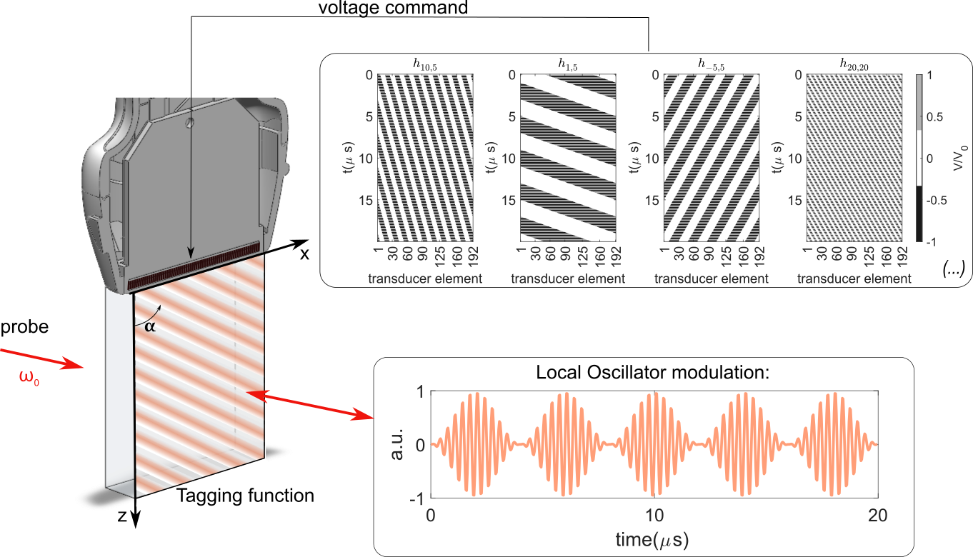
Let’s begin the description of the method as described in [3], i.e. neglecting diffraction of the propagating US. In FT-AOI, photons propagating in a scattering media are tagged by means of a long US pulse ( typically, carrier in the MHz range) periodically modulated in amplitude both along the propagation direction , and the US transducer transverse direction . The command voltage applied on a transducer array (length , composed of 192 elements) is illustrated in the top caption Fig 1, where different structurations are depicted.
The generated pressure field corresponding to the modulation with harmonics , where and are integers, can be expressed in complex form:
| (2) |
where are the coordinates of a point in the imaging plane, is the time following the emission by the transducer array, is the sound velocity, is the nominal pressure field directly set by the driving voltage , the ultrasonic carrier frequency, and where is the amplitude modulation function. The command voltage applied to the transducer is a -periodic function with a phase shift proportional to the position , with a fundamental period freely set by the user. We typically set it such that be the same order of magnitude as . If one neglects diffraction effects, the modulation function is simply obtained from using the relation:
| (3) |
with the appearing angle of the modulation illustrated in Fig 1. We perform digital off-axis holographic detection with a local oscillator (LO) centered at , where is the illumination laser carrier frequency, and modulated in amplitude by a sin-wave function with -periodicity, where a user defined phase-shift. A typical temporal profile of the LO phase modulation is illustrated at the bottom right of Fig 1 for and . Note that although other LO modulation with -periodicity could be used, the choice of sin-wave is very well-suited for the detection when accounting for the impulse response of the transducer. The weight contribution of tagged photons issued from position to the detected signal will depend on their relative phase offset with the LO. This so called "tagging function" is consequently bi-periodic in the US imaging plane as illustrated by the artistic representation in Fig 1, with a maximum contribution when both are in phase. To fetch the Fourier component of the object with frequency , where the fundamental frequencies are defined as and , we simply need to acquire four consecutive frames with respectively , from which we can estimate a complex Fourier component [3]. By repeating the process for different harmonic orders , an image is reconstructed by inverse Fourier transform. In previous work [3], an experimental reconstruction was successfully performed for and with and , corresponding to a spatial resolution of along and along . In order to improve the spatial resolution of the image along x, it is necessary to increase . Doing so however, near-field diffraction of the field known as the Talbot effect will start to manifest (typically for ), such that any attempt to increase the spatial resolution along will induce a simultaneous degradation of the reconstructed image.
3 Talbot effect in FT-AOI
To evaluate the Talbot Effect on the tagging function, we now account for diffraction in the near field of the transducer array for a given value of . The function is -periodic and can therefore be expressed as a Fourier series:
| (4) |
where the are the coefficients of the series decomposition. Here, we impose to be symmetric with respect to the origin so that are real numbers, without loss of generality. The expression of the US field in the imaging plane following the propagation can be derived using the Fresnel propagator:
| (5) |
where is the initial spatiotemporal spectrum of the emitted pressure field resulting from the amplitude modulation , defined at in Eq 3, designates the temporal frequency of the acoustic wave, the acoustic spatial frequency. In this expression, the diffraction effects are embedded in the quadratic phase function . From Eq 3 and 4 we have:
| (6) |
We inject into Eq 5 which leads to:
| (7) |
We can neglect the structuring frequencies relative to the US carrier such that . As a result, we express the modulation function defined in Eq 2 as:
| (8) |
with and . We now define the tagging function resulting from the off-axis holographic measurement by the correlation function:
| (9) |
where is the amplitude modulation function of the LO [3] and the integration time of the camera, which we impose to be a multiple of . This correlation function is essential as it represents the spatial position of the tagged photons in the insonification plane. In absence of diffraction artifacts, is a purely periodic function along both and [3]. We assume a sine-wave for the reference modulation:
| (10) |
The correlation in Eq 9 acts as a filter for the expression Eq 8. Using Eq 10 and Eq 8, we calculate the correlation function and find the following expression:
| (11) |
This simple expression allows a quite straightforward interpretation of the Talbot effect which manifests on the tagging function: it corresponds to the beating interference between the constant term and the bi-periodic structure driven by the complex coefficient . As such, a -offset on the fringes is observed for with , which corresponds to the positions:
| (12) |
Where is the Talbot distance. is plotted for and respectively in Fig 2(a) and in Fig 2(b). The half-Talbot distance is plotted In Fig 2(c) for .
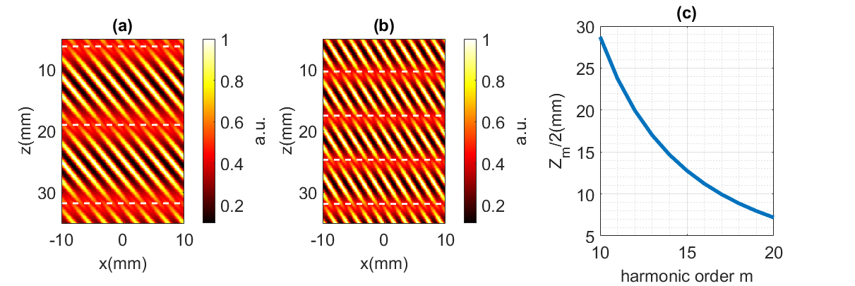
Since the imaging method further requires perform linear combinations of measurements using different values of , the extra-modulation will fundamentally deteriorates the expected Fourier component. We clearly see in Fig 2(b) that the first Talbot jump occurs at a distance which decreases with the harmonic orders . This means the degradation in imaging will be more pronounced as objects are positioned away from the probe, which is a problem for a imaging technique intended to image at large depths. We are now going to see a simple way to circumvent this problem.
3.1 -phase-jump corrections
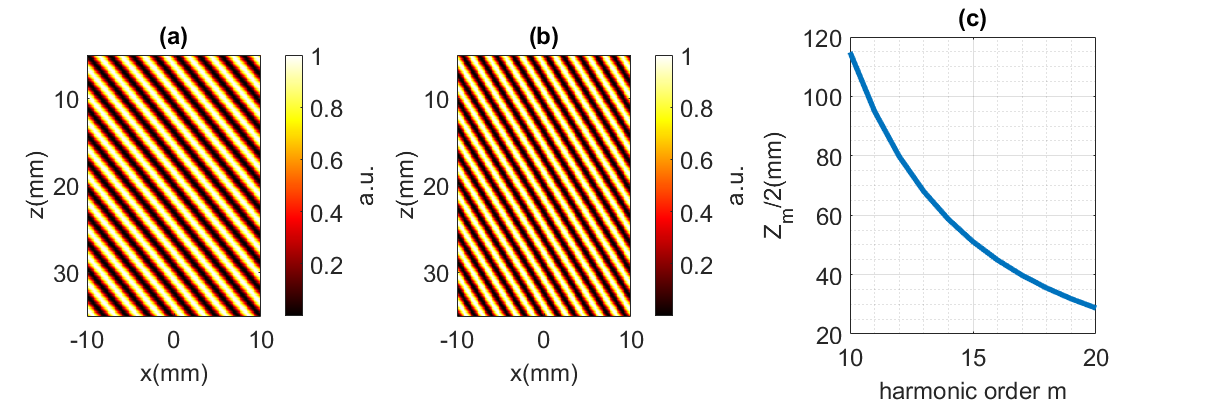
The appearance of the -shifted self-images at every half-Talbot distance from the surface can be removed by imposing an additional phase-jump modulation on the initial periodic pattern. This consists in periodically multiplying the by at the structuring frequency. The resulting modified function is now -periodic and -antiperiodic such that . Note that in this case, the Talbot distance is four times higher than in the previous case because of the quadratic dependence of with the structuration period. Although this increase in Talbot distance illustrated in Fig 4(b) could already explain an improvement in resolution for a given position below the probe, we see hereafter that this phase correction actually completely suppresses the Talbot artifact.
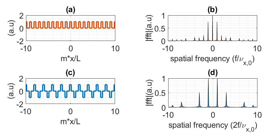
Using the previous Eq 3 at and , we obtain a similar phase-jump modulation pattern along as illustrated in Fig 3(b) for . Both respective Fourier spectra are shown in (c,d), where we see the annihilation of the even components of the spectrum when the phase correction is applied (d). Likewise, the LO originally defined by Eq 10 undergoes the same phase-jump correction so as to remain in phase with during the camera integration time. To assess the effect of this correction on the correlation function, we use the generic expression of the modulation function defined in Eq 8, and simply perform the substitution and , while recalling that we now have , the expression of the correlation function becomes:
| (13) |
Looking at Eq 13, the interpretation of the Talbot correction becomes quite straightforward: because there is no longer a constant term in the expression, the beating factor can be factorized and is equal to one once we apply the modulus. Another interpretation of this result is to consider that both the negative and positive Talbot carpets cannot be differentiated in the measurement since the modulus of a negative function is always positive. The -offset therefore does not appear as a detrimental artifact anymore, as depicted in Fig 4, where we plot the tagging function defined by Eq 13. We can now therefore extract a pure Fourier component as originally described by the method.
4 Experimental validation
We propose the simple experiment scheme depicted in Figure 5 to image the tagging functions and test our Talbot correction method. A CW laser beam centered at of propagates through a water tank sealed on each side by two optically polished silica windows. A linear transducer array, composed of 192 elements with a pitch (SL10-2 supersonic), is encoded to send long ultrasonic bursts centered at with a given modulation . The fundamental frequencies are set to and , as in [3]. A lens is positioned in the beam path to conjugate the ultrasonic imaging plane with the sensor of a digital camera (Ximea Xib-64, 300FPS). The latter beam is overlapped on the camera sensor with a LO beam centered at the tagged photons frequency and modulated in amplitude by by means of an acousto-optic modulator (not represented here), so as to perform an off-axis holographic detection. The camera exposure time is set to for all acquired frames, at a repetition rate. Each acquired image is filtered in the Fourier domain by isolating the first off-axis order resulting from the constructive interference of the tagged photons with the LO. The filtered image is then translated back into real space so that only tagged photons are visible. This allows to visualize the tagging function for a given value .
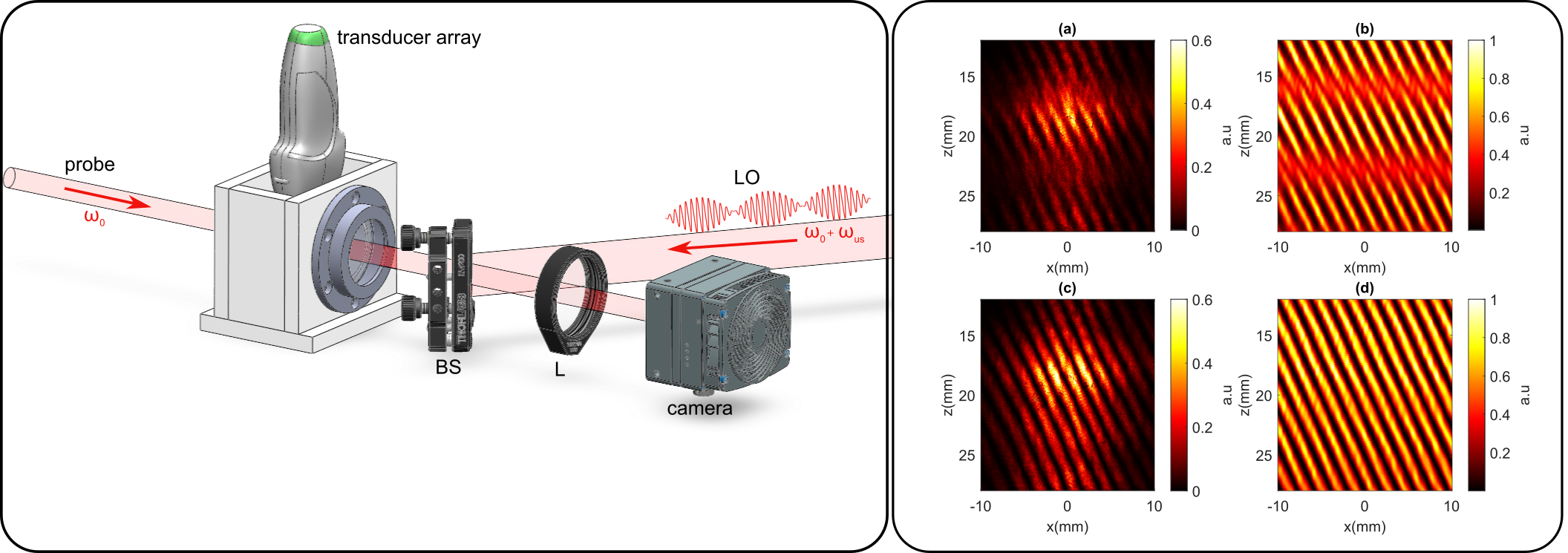
We simulate the acoustic wave propagation in water using FieldII open-source simulation software [27] already used and described in a previous work [1]. As a result, the correlation with the modulated reference beam can be computed, thereby providing a simulated image of the tagging functions for each harmonic . A comparison between the experimentally measured and the simulated tagging function is depicted on the right caption of Fig 5 for and for and . In both Fig 5 (a) and (b), where no correction is applied to the US pulse, we clearly distinguish -Talbot jumps precisely located at , as expected. By performing both the same measurement and simulation while imposing the phase jump correction on the US as previously described, we obtain Fig 5 (c) and (d) where we observe a complete suppression of this Talbot artifact. The same observation holds for all values of we have measured. Both our simulation and experimental observations are well in agreement with our previous model, thereby demonstrating the effectiveness of our correction method.
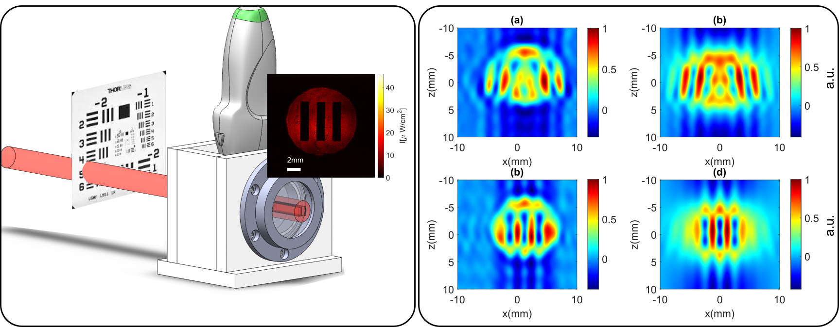
We first propose to test a full image reconstruction by inserting a resolution target (Thorlabs USAF) on vertical lines corresponding to the Group number -2 Element 5 in the beam path of the probe before it enters in the water tank. This corresponds to a line width of . This setup allows to create a test object by shadowgraphy as the resolution target is imprinted in the imaging plane defined by the position of the US transducer, as depicted in the left caption of Fig 6. The reconstructed results with (b) and without (a) Talbot correction are shown for an acquisition using , and four phases for each couple . This is a total of frames to acquire an image, leading to an acquisition time of . The corresponding simulated reconstructions are shown for comparison with (d) and without (b). The excellent qualitative agreement between the experimental and simulated reconstructions are clear evidence that the Talbot effect causes strong deformation of the image, since the target appears to be made of four rather than three lines. When the correction is applied, we observe a significant improvement of the image and the resolution target is well retrieved.
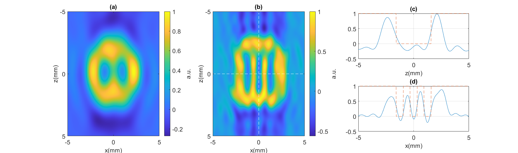
Finally, to test the limit in resolution of the method without increasing the number of components, we move the calibration target to the vertical lines with Group number -1 Element 5, which corresponds to a linewidth of , that is to say twice smaller than the one used for Fig 6. Using the same probing parameters as previously, we obtain the image Fig 7(a), which clearly shows the three vertical lines cannot be resolved. Therefore, we reiterated the experiment by doubling the fundamental frequencies used to and for the same probing values and . Doing so, we now have a resolution of along and along that compares with the ultrasonic central wavelength . The experimental reconstruction is shown in Fig 7(b) where we clearly see the three vertical lines now clearly resolved.
5 Conclusion
We have demonstrated the possibility to reach near-diffraction-limited imaging resolution using plane wave structured insonification in the context of acousto-optic imaging. So far, a limit to improving the imaging resolution along direction was the appearance of Talbot artifacts as we increased the structuring frequency along the transducer array. We have shown how imposing a -phase jump on the periodic pattern could remove this artifact without affecting the tagging function resulting from the initial US modulation. Doing so, we have improved by a factor close to ten the image resolution of our technique, reaching near-diffraction resolution. This result is an important new step towards the implementation of AO imaging based on holographic detection compatible with in-vivo decorrelation time scales. The method will be implement on living mice in a near future.
Funding French LABEX WIFI, ANR-21-CE42-0014.
Disclosures The authors declare no conflicts of interest.
Data availability Data underlying the results presented in this paper are not publicly available at this time but may be obtained from the authors upon reasonable request.
References
- [1] M. Bocoum, J.-L. Gennisson, J.-B. Laudereau, et al., “Structured ultrasound-modulated optical tomography,” \JournalTitleApplied optics 58, 1933–1940 (2019).
- [2] M. Bocoum, J.-L. Gennisson, A. A. Grabar, et al., “Reconstruction of bi-dimensional images in fourier-transform acousto-optic imaging,” \JournalTitleOptics Letters 45, 4855–4858 (2020).
- [3] L. Dutheil, M. Bocoum, M. Fink, et al., “Fourier transform acousto-optic imaging with off-axis holographic detection,” \JournalTitleApplied optics 60, 7107–7112 (2021).
- [4] M. M. Qureshi, J. Brake, H.-J. Jeon, et al., “In vivo study of optical speckle decorrelation time across depths in the mouse brain,” \JournalTitleBiomedical optics express 8, 4855–4864 (2017).
- [5] Y. Liu, P. Lai, C. Ma, et al., “Optical focusing deep inside dynamic scattering media with near-infrared time-reversed ultrasonically encoded (true) light,” \JournalTitleNature communications 6, 5904 (2015).
- [6] Z. Cheng, C. Li, A. Khadria, et al., “High-gain and high-speed wavefront shaping through scattering media,” \JournalTitleNature Photonics pp. 1–7 (2023).
- [7] H. F. Talbot, “Lxxvi. facts relating to optical science. no. iv,” \JournalTitleThe London, Edinburgh, and Dublin Philosophical Magazine and Journal of Science 9, 401–407 (1836).
- [8] J. R. Leger, “Lateral mode control of an AlGaAs laser array in a talbot cavity,” \JournalTitleApplied physics letters 55, 334–336 (1989).
- [9] J. R. Leger, M. L. Scott, and W. B. Veldkamp, “Coherent addition of AlGaAs lasers using microlenses and diffractive coupling,” \JournalTitleApplied physics letters 52, 1771–1773 (1988).
- [10] D. Mehuys, W. Streifer, R. G. Waarts, and D. F. Welch, “Modal analysis of linear talbot-cavity semiconductor lasers,” \JournalTitleOptics letters 16, 823–825 (1991).
- [11] S. Chowdhury, J. Chen, and J. A. Izatt, “Structured illumination fluorescence microscopy using talbot self-imaging effect for high-throughput visualization,” \JournalTitlearXiv preprint arXiv:1801.03540 (2018).
- [12] L. Stuerzebecher, T. Harzendorf, U. Vogler, et al., “Advanced mask aligner lithography: fabrication of periodic patterns using pinhole array mask and talbot effect,” \JournalTitleOptics express 18, 19485–19494 (2010).
- [13] L. Wang, F. Clube, C. Dais, et al., “Sub-wavelength printing in the deep ultra-violet region using displacement talbot lithography,” \JournalTitleMicroelectronic Engineering 161, 104–108 (2016).
- [14] L. Rayleigh, “Xxv. on copying diffraction-gratings, and on some phenomena connected therewith,” \JournalTitleThe London, Edinburgh, and Dublin Philosophical Magazine and Journal of Science 11, 196–205 (1881).
- [15] M. R. Dennis, N. I. Zheludev, and F. J. G. De Abajo, “The plasmon talbot effect,” \JournalTitleOptics Express 15, 9692–9700 (2007).
- [16] M. S. Chapman, C. R. Ekstrom, T. D. Hammond, et al., “Near-field imaging of atom diffraction gratings: The atomic talbot effect,” \JournalTitlePhysical Review A 51, R14 (1995).
- [17] J. F. Clauser and S. Li, “Talbot-vonlau atom interferometry with cold slow potassium,” \JournalTitlePhysical Review A 49, R2213 (1994).
- [18] L. Deng, E. W. Hagley, J. Denschlag, et al., “Temporal, matter-wave-dispersion talbot effect,” \JournalTitlePhysical Review Letters 83, 5407 (1999).
- [19] A. N. Morozov, M. P. Krikunova, B. Skuibin, and E. V. Smirnov, “Observation of the talbot effect for ultrasonic waves,” \JournalTitleJETP Letters 106, 23–25 (2017).
- [20] P. Candelas, J. M. Fuster, S. Pérez-López, et al., “Observation of ultrasonic talbot effect in perforated plates,” \JournalTitleUltrasonics 94, 281–284 (2019).
- [21] P. Latimer and R. F. Crouse, “Talbot effect reinterpreted,” \JournalTitleApplied optics 31, 80–89 (1992).
- [22] M. Berry, I. Marzoli, and W. Schleich, “Quantum carpets, carpets of light,” \JournalTitlePhysics World 14, 39 (2001).
- [23] J. Wen, Y. Zhang, and M. Xiao, “The talbot effect: recent advances in classical optics, nonlinear optics, and quantum optics,” \JournalTitleAdvances in optics and photonics 5, 83–130 (2013).
- [24] K. Pelka, J. Graf, T. Mehringer, and J. von Zanthier, “Prime number decomposition using the talbot effect,” \JournalTitleOptics Express 26, 15009–15014 (2018).
- [25] H. G. De Chatellus, E. Lacot, W. Glastre, et al., “Theory of talbot lasers,” \JournalTitlePhysical Review A 88, 033828 (2013).
- [26] L. Romero Cortés, R. Maram, H. Guillet de Chatellus, and J. Azaña, “Arbitrary energy-preserving control of optical pulse trains and frequency combs through generalized talbot effects,” \JournalTitleLaser & photonics reviews 13, 1900176 (2019).
- [27] J. A. Jensen, “A model for the propagation and scattering of ultrasound in tissue,” \JournalTitleThe Journal of the Acoustical Society of America 89, 182–190 (1991).