Integral representations and zeros of the Lommel function and the hypergeometric ${}_{1}F_{2}$ function.

Abstract

We give different integral representations of the Lommel function $s_{\mu,\nu}(z)$ involving trigonometric and hypergeometric ${}_{2}F_{1}$ functions. By using classical results of Polya, we give the distribution of the zeros of $s_{\mu,\nu}(z)$ for certain regions in the plane $(\mu,\nu)$. Further, thanks to a well known relation between the functions $s_{\mu,\nu}(z)$ and the hypergeometric ${}_{1}F_{2}$ function, we describe the distribution of the zeros of ${}_{1}F_{2}$ for specific values of its parameters.

1 Introduction

The Lommel function $s_{\mu,\nu}(z)$ is a particular solution of the inhomogeneous Bessel differential equation:

$$z^{2}\frac{d^{2}y}{dz^{2}}+z\frac{dy}{dz}+(z^{2}-\nu^{2})y=z^{\mu+1}.$$ (1)

More precisely, $s_{\mu,\nu}(z)$ is the solution of equation (1) satisfying $s_{\mu,\nu}(z)\sim\frac{z^{\mu+1}}{(\mu+1)^{2}-\nu^{2}}(1+O(z^{2}))$ around $z=0$ when $\mu\pm\nu$ is not an odd negative integer. The explicit Taylor series of $s_{\mu,\nu}(z)$ around $z=0$ is given by [21]

$$s_{\mu,\nu}(z)=\frac{z^{\mu+1}}{(\mu+1)^{2}-\nu^{2}}\left(1-\frac{z^{2}}{(\mu+3)^{2}-\nu^{2}}+\frac{z^{4}}{\left((\mu+3)^{2}-\nu^{2}\right)\left((\mu+5)^{2}-\nu^{2}\right)}+\cdots\right)$$ (2)

The previous expression can be equivalently written in terms of hypergeometric ${}_{1}F_{2}$ function as [21]

$$s_{\mu,\nu}(z)=\frac{z^{\mu+1}}{(\mu+1)^{2}-\nu^{2}}\,_{1}F_{2}\left(1;\frac{\mu-\nu+3}{2},\frac{\mu+\nu+3}{2};-\frac{z^{2}}{4}\right)$$ (3)

Notice that the function ${}_{1}F_{2}$ in (3), or $z^{-\mu-1}s_{\mu,\nu}(z)$, is an entire function of $z$ with order of growth equal to 1. The Lommel function has many applications in mathematical physics and applied sciences: for example, it is fundamental in the description of piezoelectricity phenomena [1], optics [2], radiative transfer processes in the atmosphere [3], mechanics [15], elastic scattering theory [19].

In this paper we will analyze the distribution of the zeros of the function $s_{\mu,\nu}(z)$. The identification of the values $(\mu,\nu)$ giving a non negative function $s_{\mu,\nu}(z)$ on the real axis and the description of the location of the zeros have been investigated by many authors. In [5] Cooke showed that if $\nu\geq 0$ and $\nu\leq\mu-1$ then $s_{\mu,\nu}(z)>0$ for $z>0$. Equally, if $\nu\geq 1/2$ and $\nu\leq\mu$ $s_{\mu,\nu}(z)>0$ for $z>0$, unless $\mu=\nu=1/2$ when $s_{\mu,\nu}\geq 0$ for $z>0$. Successively, Steinig [16] showed that $s_{\mu,\nu}(z)>0$ for $z>0$ if $|\nu|<\mu$ and $\mu\geq 1/2$ except when $|\nu|=\mu=1/2$, where one has $s_{\mu,\nu}(z)\geq 0$ for $z>0$. Also, Steinig established the following properties of $s_{\mu,\nu}(z)$: if $\mu<1/2$ or if $\mu=1/2$ and $|\nu|>1/2$ then $s_{\mu,\nu}(z)$ has an infinite number of zeros for $z\in(0,\infty)$. An extension of the positivity results of Cooke and Steinig has been given more recently by Cho & Chung [4], since they showed that $s_{\mu,\nu}>0$ also in the region $\mu>1/2$ and $\nu^{2}\leq(\mu+1)^{2}-2$, whereas $s_{\mu,\nu}\geq 0$ for $\mu=|\nu|=1/2$, giving also interlacing properties among the zeros of $s_{\mu,\nu}$ and those of the Bessel function $J_{\nu}$ for certain values of the parameters $(\mu,\nu)$. In [12] Koumandos and Lamprecht give estimates about the location of the zeros of $s_{\mu,\nu}(z)$ for $\mu\in(-1/2,1/2)$ and $\nu=1/2$, whereas in [11] Koumandos, extends these to $\mu\in(-3/2,1/2)$, $\mu\neq-1/2$ and $\nu=1/2$.

One of the tools that we will use is a result due to Polya [14] about the zeros of entire functions possessing suitable integral representations. The theorem is the following:

Theorem 1.1

[Polya, 1918 [14]] Suppose that the function $f(t)$ is positive and not decreasing in $(0,1)$. Then the functions of $z$ defined by

$$V(z)=\int_{0}^{1}\sin(zt)f(t)dt,\quad U(z)=\int_{0}^{1}\cos(zt)f(t)dt$$ (4)

possesses only real zeros. Further, if $f(t)$ grows steadily these zeros are simple and the intervals $(k\pi,(k+1)\pi)$, $k=1,2,\ldots$ contain the positive zeros of $V(z)$, whereas the intervals $(\frac{(2k+1)\pi}{2},\frac{(2k+3)\pi}{2})$, $k=0,1,2,\ldots$ contain the zeros of $U(z)$, each interval containing just one zero in both cases.

By growing steadily it is meant that the function is not piecewise constant with a finite number of rational points of discontinuity in $(0,1)$.

2 Some integral representations and comments

In this section we will report some known facts about integral representations of the function $s_{\mu,\nu}(z)$. In particular, in 1936 Szymanski [18] got an integral representation for the Lommel function in the case $\nu-\mu$ is an even positive integer. Actually, Szymanski firstly considers equation (1) for imaginary argument:

$$z^{2}\frac{d^{2}T}{dz^{2}}+z\frac{dT}{dz}-(z^{2}+\nu^{2})T=z^{\mu+1}.$$ (5)

and noticed that the solution of (5) satisfying $T=t_{\mu,\nu}(z)\sim\frac{z^{\mu+1}}{(\mu+1)^{2}-\nu^{2}}(1+O(z))$ can be expressed as

$$t_{\mu,\nu}=z^{\mu+1}\int_{0}^{1}\cosh(zt)W_{\mu,\nu}(t)dt,$$ (6)

where $W_{\mu,\nu}$ is the solution of the following differential equation

$$(1-t^{2})\frac{d^{2}W_{\mu,\nu}}{dt^{2}}+(2\mu-1)t\frac{dW_{\mu,\nu}}{dt}+(\nu^{2}-\mu^{2})W_{\mu,\nu}=0,$$ (7)

with the following boundary conditions

$$W(1)=0,\quad W^{\prime}(0)=-1.$$ (8)

The solution of equation (7) with the boundary conditions (8) is written by Szymanski in terms of the Gegenbauer functions $C_{n}^{k}$:

$$W_{\mu,\nu}(t)=-(1-t^{2})^{\mu+\frac{1}{2}}\frac{C_{\nu-\mu-1}^{\mu+1}(t)}{\left(C_{\nu-\mu-1}^{\mu+1}(t)\right)^{\prime}_{t=0}}.$$ (9)

where, for integers values of $\nu-\mu-1$ (odd values, for even positive integers the denominator vanishes), the functions $C_{n}^{k}$ are defined by the generating function $(1-2xt+x^{2})^{-k}$, i.e. $C_{n}^{k}(t)$ is the coefficients of $x^{n}$ in the expansion of $(1-2xt+x^{2})$ in powers of $x$:

$$(1-2xt+x^{2})^{-k}=\sum_{n=0}C_{n}^{k}(t)x^{n}.$$ (10)

For the solution $s_{\mu,\nu}(z)$ of (1) equally one finds, for $\nu-\mu$ even integers:

$$s_{\mu,\nu}=z^{\mu+1}\int_{0}^{1}\cos(zt)W_{\mu,\nu}(t)dt,$$ (11)

where $W_{\mu,\nu}(t)$ is again given by the expression (9).

In [22] another integral representation of the function $s_{0,v}(z)$ is given. In particular, by a direct check, it is possible to show that the function

$$s_{0,\nu}(z)=\frac{1}{1+\cos(\pi\nu)}\int_{0}^{\pi}\sin(z\sin(t))\cos(\nu t)dt.$$ (12)

solves equation (1) when $\mu=0$ with $s_{0,\nu}(z)\sim\frac{z}{1-\nu^{2}}(1+O(z))$. Equivalently, the function $s_{0,\nu}(z)$ can be also represented as

$$s_{0,\nu}(z)=\frac{1}{1+\cos(\pi\nu)}\int_{0}^{1}\sin(zt)\frac{\cos(\nu\arcsin(t))+\cos(\nu\pi-\nu\arcsin(t))}{\sqrt{1-t^{2}}}dt,$$ (13)

where the range of $\arcsin$ is $(-\pi/2,\pi/2)$. It is possible to show that the function multiplying $\sin(zt)$ in (13) is positive and increasing for $|\nu|<1$ and $t\in(0,1)$. It is then possible to apply the Theorem (1.1) to get the following

Corollary 2.1

The function $s_{0,\nu}(z)$, for $|\nu|<1$, possesses only real zeros. The zeros are simple and the intervals $(k\pi,(k+1)\pi)$, $k=0,1,2,\ldots$ contain the non-negative zeros of $s_{0,\nu}(z)$, each interval containing just one zero.

In the next section we will extend the integral representation (12) and the results described in Corollary (2.1) to other values of $\mu$.

3 Other integral representations and the zeros

In this section we will assume that $\mu\pm\nu$ is not an odd negative integer so that the series (2) is defined. By generalizing the case $\mu=0$ considered in [22], we make the following ansatz for the function $s_{\mu,\nu}(z)$:

$$s_{\mu,\nu}(z)=z^{\mu}\int_{0}^{1}\sin(zt)f_{\mu,\nu}(t)dt.$$ (14)

We assume that the functions $f_{\mu,\nu}(t)$ are finite in $z=0$ whereas may be unbounded for $t\to 1$. By inserting (14) in (1) we get that the functions $f_{\mu,\nu}(t)$ must be the solutions of the following differential equations

$$(1-t^{2})\frac{d^{2}f_{\mu,\nu}}{dt^{2}}+(2\mu-3)t\frac{df_{\mu,\nu}}{dt}+(\nu^{2}-(\mu-1)^{2})f_{\mu,\nu}=0,$$ (15)

with the boundary conditions:

$$f_{\mu,\nu}(0)=1,\quad\lim_{t\to 1^{-}}(1-t)f_{\mu,\nu}(t)=0,\quad\lim_{t\to 1^{-}}\left((1-t^{2})\frac{df_{\mu,\nu}}{dt}+(2\mu-1)tf_{\mu,\nu}\right)=0.$$ (16)

The general solution of equation (15) can be represented in terms of hypergeometric functions as:

$$A(1-t)^{\mu-\frac{1}{2}}\,_{2}F_{1}\left(\frac{1}{2}+\nu,\frac{1}{2}-\nu;\mu+\frac{1}{2};\frac{1-t}{2}\right)+B\,_{2}F_{1}\left(1-\nu-\mu,1+\nu-\mu;\frac{3}{2}-\mu;\frac{1-t}{2}\right)$$ (17)

where $A$ and $B$ are two arbitrary constants. The condition $\lim_{t\to 1^{-}}(1-t)f_{\mu,\nu}(t)=0$ gives

$$\mu+\frac{1}{2}>0,$$ (18)

whereas the series around $t=1$ of the function $(1-t^{2})\frac{df_{\mu,\nu}}{dt}+(2\mu-1)tf_{\mu,\nu}$ is given by

$$(1-t^{2})\frac{df_{\mu,\nu}}{dt}+(2\mu-1)tf_{\mu,\nu}\sim\left(A(1-t)^{\mu+\frac{1}{2}}\frac{\nu^{2}-\mu^{2}}{2\mu+1}+B(2\mu+1)\right)\left(1+O(1-t)\right),$$ (19)

and results in $B=0$. Finally, from the boundary condition (16) $f_{\mu,\nu}(0)=1$ we get

$$A\,_{2}F_{1}\left(\frac{1}{2}+\nu,\frac{1}{2}-\nu;\mu+\frac{1}{2};\frac{1}{2}\right)=1.$$ (20)

The previous result is summarized in the following

Proposition 3.1

For $\mu>-\frac{1}{2}$ the Lommel function $s_{\mu,\nu}(z)$ possess the following integral representation:

$$s_{\mu,\nu}(z)=z^{\mu}\int_{0}^{1}\sin(zt)f_{\mu,\nu}(t)dt=z^{\mu}\int_{0}^{1}\frac{\sin(zt)}{(1-t)^{\frac{1}{2}-\mu}}\frac{{}_{2}F_{1}\left(\frac{1}{2}+\nu,\frac{1}{2}-\nu;\mu+\frac{1}{2};\frac{1-t}{2}\right)}{{}_{2}F_{1}\left(\frac{1}{2}+\nu,\frac{1}{2}-\nu;\mu+\frac{1}{2};\frac{1}{2}\right)}dt.$$ (21)

We are interested in the monotonicity of the integrand $f_{\mu,\nu}(t)$ for $t\in(0,1)$ and $\mu>-1/2$. We notice that the derivative of $f_{\mu,\nu}$ with respect to $t$ is proportional again to a hypergeometric function:

$$\frac{df_{\mu,\nu}}{dt}=\frac{1-2\mu}{2(1-t)^{\frac{3}{2}-\mu}}\frac{{}_{2}F_{1}\left(\frac{1}{2}+\nu,\frac{1}{2}-\nu;\mu-\frac{1}{2};\frac{1-t}{2}\right)}{{}_{2}F_{1}\left(\frac{1}{2}+\nu,\frac{1}{2}-\nu;\mu+\frac{1}{2};\frac{1}{2}\right)}.$$ (22)

The previous relation can be written in a more compact form as

$$\frac{df_{\mu,\nu}}{dt}+a_{\mu,\nu}f_{\mu-1,\nu}=0,$$ (23)

where we set

$$a_{\mu,\nu}\doteq 2\frac{\Gamma\left(\frac{\mu+1+\nu}{2}\right)\Gamma\left(\frac{\mu+1-\nu}{2}\right)}{\Gamma\left(\frac{\mu+\nu}{2}\right.)\Gamma\left(\frac{\mu-\nu}{2}\right)}.$$ (24)

Notice that $a_{\mu,\nu}$ is related to the integral of $f_{\mu,\nu}(t)$ between $0$ and $1$: indeed, from (23) we get for $\mu+1/2>0$

$$\int_{0}^{1}f_{\mu,\nu}(t)dt=\frac{1}{a_{\mu+1,\nu}}=\frac{\Gamma\left(\frac{\mu+1+\nu}{2}\right)\Gamma\left(\frac{\mu+1-\nu}{2}\right)}{2\Gamma\left(\frac{\mu+\nu}{2}+1\right.)\Gamma\left(\frac{\mu-\nu}{2}+1\right)}.$$ (25)

The previous quantity is finite under the given assumptions that $\mu\pm\nu$ is not an odd negative integer.

As regards the monotonicity, from (23) we see that the zeros of $\frac{df_{\mu,\nu}}{dt}$ between $0$ and $1/2$ are the zeros of ${}_{2}F_{1}\left(\frac{1}{2}+\nu,\frac{1}{2}-\nu;\mu-\frac{1}{2};\frac{1-t}{2}\right)$, since the constant coefficient is zero only for $\mu+\frac{1}{2}=-n$, $n=0,1,2,...$ as can be seen directly from the explicit expression

$${}_{2}F_{1}\left(\frac{1}{2}+\nu,\frac{1}{2}-\nu;\mu+\frac{1}{2};\frac{1}{2}\right)=2^{1/2-\mu}\sqrt{\pi}\frac{\Gamma(\mu+\frac{1}{2})}{\Gamma(\frac{\mu+\nu+1}{2})\Gamma(\frac{\mu-\nu+1}{2})}$$ (26)

The number of zeros of the hypergeometric functions ${}_{2}F_{1}(a,b;c;x)$ for $x\in(0,1)$ have been analyzed by Klein [10] and Hurwitz [9]. For completeness, we report these results as given by Hurwitz. They are summarized in Table (1) for $a>b$, $c\leq a+b$

$a$	$b$	$c$	$N$
+	+	+	0
+	+	-	$\frac{1+(-1)^{\lfloor-c\rfloor}}{2}$
+	-	+	$1+\lfloor-b\rfloor$
+	-	-	$\lfloor-b\rfloor-\lfloor-c\rfloor$, for $\lfloor-b\rfloor>\lfloor-c\rfloor$
+	-	-	$\frac{1-(-1)^{\lfloor-b\rfloor+\lfloor-c\rfloor}}{2}$, for $\lfloor-b\rfloor\leq\lfloor-c\rfloor$
-	-	-	$\frac{1+(-1)^{\lfloor-a\rfloor+\lfloor-b\rfloor+\lfloor-c\rfloor}}{2}$

Table 1: The number of zeros $N$ of ${}_{2}F_{1}(a,b;c;x)$ for $x\in(0,1)$, $a>b$, $c\leq a+b$.

We notice however that from table (1) we can provide only partial results about the region of the parameters $(\nu,\mu)$ where the function
${}_{2}F_{1}\left(\frac{1}{2}+\nu,\frac{1}{2}-\nu;\mu-\frac{1}{2};\frac{1-t}{2}\right)$ is free from zeros for $t\in(0,1)$. Indeed, the table (1) gives this information for $t\in(-1,1)$. We need to extend the results of Hurwitz and Klein and look at the zeros of ${}_{2}F_{1}(a,b;c;x)$ in the region $x\in(0,1/2)$, i.e. the zeros of ${}_{2}F_{1}\left(\frac{1}{2}+\nu,\frac{1}{2}-\nu;\mu-\frac{1}{2};\frac{1-t}{2}\right)$ for $t\in(0,1)$. To this aim, the quadratic (in the independent variable) functional identities for the hypergeometric functions are very useful. The identity we need is the following (see [7], formula 41 at page 120):

$$\frac{{}_{2}F_{1}\left(\frac{1}{2}+\nu,\frac{1}{2}-\nu;\mu-\frac{1}{2};x\right)}{(1-2x)\left(1-x\right)^{\mu-3/2}}=\,_{2}F_{1}\left(\frac{\mu+\nu}{2},\frac{\mu-\nu}{2};\mu-\frac{1}{2};4x(1-x)\right)$$ (27)

where $x\in(0,1/2)$. Equation (27) provides an explicit relation between the zeros of ${}_{2}F_{1}\left(\frac{\mu+\nu}{2},\frac{\mu-\nu}{2};\mu-\frac{1}{2};x\right)$ and the zeros of ${}_{2}F_{1}\left(\frac{1}{2}+\nu,\frac{1}{2}-\nu;\mu-\frac{1}{2};x\right)$. In particular it follows that if ${}_{2}F_{1}\left(\frac{\mu+\nu}{2},\frac{\mu-\nu}{2};\mu-\frac{1}{2};x\right)$ is free from zeros for $x\in(0,1)$, ${}_{2}F_{1}\left(\frac{1}{2}+\nu,\frac{1}{2}-\nu;\mu-\frac{1}{2};x\right)$ is free from zeros for $x\in(0,1/2)$. By looking at table (1) for ${}_{2}F_{1}\left(\frac{\mu+\nu}{2},\frac{\mu-\nu}{2};\mu-\frac{1}{2};x\right)$ we get the following

Proposition 3.2

For $\mu>-1/2$ the function $f_{\mu,\nu}(t)$ is monotonic for $t\in(0,1)$ iff the following conditions on the parameters are satisfied:

• $\mu>1/2$ and $|\nu|\in(0,\mu)$.

• $\mu<1/2$ and $|\nu|\in(|\mu|,\mu+2)$

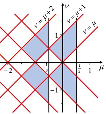
Figure 2: The regions described in Corollary (3.4) and Corollary (3.9).

The region in the plane $(\mu,\nu)$ corresponding to monotonic function $f_{\mu,\nu}(t)$ for $t\in(0,1)$ is illustrated in figure (2).

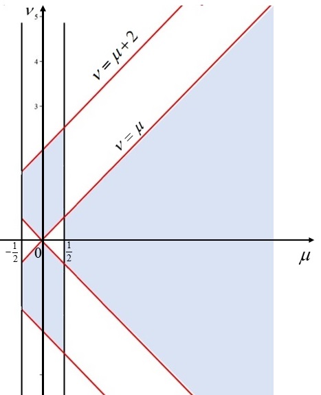
Figure 1: The region of monotonicity of $f_{\mu,\nu}(t)$ for $t\in(0,1)$.

The function $f_{\mu,\nu}(t)$ can be decreasing or increasing for $t\in(0,1)$. Since $f_{\mu,\nu}(0)=1$, by looking at what happens in a neighborhood of $t=1$ it is simple to get the following

Proposition 3.3

For $\mu>-1/2$ the function $f_{\mu,\nu}(t)$ has the following monotonicity properties going from $t=0$ to $t=1$:

• For $\mu>1/2$ and $|\nu|\in(0,\mu)$ the function is decreasing from 1 to 0.

• For $\mu<1/2$ and $|\nu|\in(|\mu|,\mu+1)$ the function is increasing from 1 to $+\infty$.

• For $\mu<1/2$ and $|\nu|\in(\mu+1,\mu+2)$ the function is decreasing from 1 to $-\infty$.

From Proposition (3.3) and Theorem (1.1) we immediately get the following

Corollary 3.4

Apart the branch point at $z=0$, the function $s_{\mu,\nu}(z)$ for $\mu\in(-1/2,1/2)$ and $|\nu|\in(|\mu|,\mu+1)$ possesses only real zeros. The zeros are simple and the intervals $(k\pi,(k+1)\pi)$, $k=1,2,\ldots$ contain the non-negative zeros, each interval containing just one zero.

The previous generalizes the Corollary (2.1) given in [22]. Further, since for $\mu>1/2$ and $|\nu|\in(0,\mu)$ the function $f_{\mu,\nu}(t)$ is positive and decreasing, we get the Corollary:

Corollary 3.5

The function $s_{\mu,\nu}(z)$ for $\mu>1/2$ and $|\nu|\in(0,\mu)$ is positive on the positive real axis and possesses only complex zeros.

Corollary (3.5) is not new, it has been given by [16] and then appears in [6]. The proof given here is however simpler. The zeros of $s_{\mu,\nu}(z)$ can be better characterized by looking at the asymptotic expansion of the hypergeometric ${}_{1}F_{2}$ function, related to $s_{\mu,\nu}(z)$ by the formula (3). Indeed, by using the results given in [13] and with the aid of (3) we get, for $z$ real and positive, the asymptotic relation

$$\frac{s_{\mu,\nu}(z)}{z^{\mu+1}}\sim\frac{1}{z^{2}}\left(1+O(\frac{1}{z})\right)+\frac{\Gamma\left(\frac{\mu+\nu+1}{2}\right)\Gamma\left(\frac{\mu-\nu+1}{2}\right)}{4\sqrt{\pi}}\left(\frac{2}{z}\right)^{\mu+\frac{3}{2}}\cos\left(z-\frac{\pi}{2}(\mu+\frac{3}{2})\right)(1+O(\frac{1}{z}))$$ (28)

and if $\mu<1/2$ we see that the zeros are asymptotically given by $z_{k}\sim\pi\left(k+\frac{2\mu+5}{4}\right)$, for $k$ suitable large integers.

The behavior of $f_{\mu,\nu}(t)$ for $t\in(0,1)$, $\mu\in(-1/2,1/2)$ and $|\nu|\in(\mu+1,\mu+2)$ gives the following result: yhe function $c-f_{\mu,\nu}(t)$ is positive and increasing for $t\in(0,1)$ for any $c\geq 1$. Indeed, if we introduce the function

$$V_{\mu,\nu}(z)\doteq z^{\mu}\int_{0}^{1}(c-f_{\mu,\nu}(t))\sin(zt)dt=z^{\mu-1}c(1-\cos(z))-s_{\mu,\nu}(z),$$ (29)

we can apply the Polya Theorem (1.1) and get the following

Corollary 3.6

For any $c\geq 1$, the function $V_{\mu,\nu}(z)=cz^{\mu-1}(1-\cos(z))-s_{\mu,\nu}(z)$ for $\mu\in(-1/2,1/2)$ and $|\nu|\in(\mu+1,\mu+2)$ possesses only real zeros. The zeros are simple and the intervals $(k\pi,(k+1)\pi)$, $k=1,2,\ldots$ contain the non-negative zeros, each interval containing just one zero.

Actually, (21) is not the only integral representation in terms of a trigonometric kernel. Indeed, it is also possible to give a cosine integral representation. Let us assume $\mu>1/2$. Then, by integrating by parts equation (21) we get

$$s_{\mu,\nu}=z^{\mu}\left(\frac{1}{z}-\frac{a_{\mu,\nu}}{z}\int_{0}^{1}\cos(zt)f_{\mu-1,\nu}(t)\right),$$ (30)

where we used equation (23). Let us set

$$c_{\mu,\nu}\doteq z^{\mu+1}a_{\mu+1,\nu}\int_{0}^{1}\cos(zt)f_{\mu,\nu}(t).$$ (31)

Equation (31) is well defined for $\mu>-1/2$. Again, by integrating by parts (31) and by using the equation $a_{\mu+1,\nu}a_{\mu,\nu}=(\mu^{2}-\nu^{2})$ we get, for $\mu>+1/2$

$$c_{\mu,\nu}=z^{\mu}\left(\mu^{2}-\nu^{2}\right)\int_{0}^{1}\sin(zt)f_{\mu-1,\nu}(t)=(\mu^{2}-\nu^{2})zs_{\mu-1,\nu}.$$ (32)

From (32) it follows that, for $\mu>-1/2$

$$s_{\mu,\nu}=\frac{1}{z((\mu+1)^{2}-\nu^{2})}c_{\mu+1,\nu}=\frac{a_{\mu+2,\nu}}{((\mu+1)^{2}-\nu^{2})}z^{\mu+1}\int_{0}^{1}\cos(zt)f_{\mu+1,\nu}(t).$$ (33)

Notice that the previous integral representation is still convergent for $\mu>-3/2$. It is also possible to check directly, by using the series for the hypergeometric function around $t=1$ that indeed the integral in (33) gives $s_{\mu,\nu}$ also for $\mu\in(-3/2,-1/2)$, so we get the following

Proposition 3.7

For $\mu>-\frac{3}{2}$ the Lommel function $s_{\mu,\nu}(z)$ possesses the following integral representation:

$$s_{\mu,\nu}(z)=\frac{a_{\mu+2,\nu}}{((\mu+1)^{2}-\nu^{2})}z^{\mu+1}\int_{0}^{1}\cos(zt)f_{\mu+1,\nu}(t)=\frac{z^{\mu+1}}{a_{\mu+1,\nu}}\int_{0}^{1}\cos(zt)f_{\mu+1,\nu}(t).$$ (34)

where $a_{\mu,\nu}$ is given in equation (24) and $f_{\mu,\nu}(t)$ by equation (21).

It is possible to get the integral representation (34) also by directly making the ansatz $s_{\mu,\nu}=z^{\mu+1}\int_{0}^{1}\cos(zt)f(t)$ for some $f(t)$ and then by looking at the differential equation and boundary conditions that $f(t)$ must obey so that $s_{\mu,\nu}$ satisfies equation (1), like we did with the integral representation (21). Since in the integral (34) it appears the function $f_{\mu+1,\nu}(t)$, i.e. the same function appearing in the integral (21) but with $\mu\to\mu+1$, from Proposition (3.7) we get directly the following

Proposition 3.8

For $\mu>-3/2$ the function $f_{\mu+1,\nu}(t)$ is monotonic for $t\in(0,1)$ iff the following conditions on the parameters are satisfied:

• $\mu>-1/2$ and $|\nu|\in(0,\mu+1)$.

• $\mu<-1/2$ and $|\nu|\in(|\mu+1|,\mu+3)$

To understand the behavior of $\frac{f_{\mu+1,\nu}(t)}{a_{\mu+1,\nu}}$, we look at the end-points $t=0$ and $t=1$. For $t=0$ we get

$$\frac{f_{\mu+1,\nu}(0)}{a_{\mu+1,\nu}}=\frac{1}{a_{\mu+1,\nu}}=\frac{\Gamma\left(\frac{\mu+1+\nu}{2}\right)\Gamma\left(\frac{\mu+1-\nu}{2}\right)}{2\Gamma\left(1+\frac{\mu+\nu}{2}\right.)\Gamma\left(1+\frac{\mu-\nu}{2}\right)}$$ (35)

For $\mu>-1/2$ $f_{\mu+1,\nu}(1)=0$, giving a decreasing function for $|\nu|\in(0,\mu+1)$ since the values of the function (35) is positive in this interval. For $\mu<-1/2$ $f_{\mu+1,\nu}(t)$ diverges at $t=1$, the sign being negative. Also, for $|\nu|\in(|\mu+1|,\mu+2)$ the values of the function (35) are negative, whereas for $|\nu|\in(\mu+2,\mu+3)$ are positive. It follows that the function

$$-\frac{1}{a_{\mu+1,\nu}}f_{\mu+1,\nu}(t)$$ (36)

is positive and increasing for $\mu\in(-3/2,-1/2)$ and $|\nu|\in(|\mu+1|,\mu+2)$. The previous results let to expand the region in the $(\mu,\nu)$ plane for the Corollary (3.4). Indeed we immediately get the following

Corollary 3.9

Apart the branch point at $z=0$, the function $s_{\mu,\nu}(z)$ for $\mu\in(-3/2,-1/2)$ and $|\nu|\in(|\mu+1|,\mu+2)$ possesses only real zeros. The zeros are simple and the intervals $(\frac{(2k+1)\pi}{2},\frac{(2k+3)\pi}{2})$, $k=0,1,2,\ldots$ contain the non-negative zeros, each interval containing just one zero.

With the same considerations given after Corollary (3.5) it is possible to show that the zeros in Corollary (3.9) are asymptotically given by $z_{k}\sim\pi\left(k+\frac{2\mu+5}{4}\right)$ for large $k$.

As we did with Corollary (3.6), we can introduce the function

$$U_{\mu,\nu}(z)=z^{\mu}(c+\frac{1}{a_{\mu+1,\nu}})\sin(z)-s_{\mu,\nu}(z),$$ (37)

and, from the Polya Theorem (1.1) we get the following

Corollary 3.10

For any $c\geq 0$, the function $U_{\mu,\nu}(z)$ (37) for $\mu\in(-3/2,-1/2)$ and $|\nu|\in(\mu+2,\mu+3)$ or $\mu>-1/2$ and $|\nu|\in(0,\mu+1)$ possesses only real zeros. The zeros are simple and the intervals $(\frac{(2k+1)\pi}{2},\frac{(2k+3)\pi}{2})$, $k=0,1,2,\ldots$ contain the non-negative zeros, each interval containing just one zero.

The Corollaries (3.6) and (3.10) are trivial when the value of $c$ is large and for large real values of $z$, due to the asymptotic (28). They are less obvious for smaller values of $z$.

By looking closer at the paper [14], one sees that Theorem (1.1) can be actually extended to linear combinations of the functions $U(z)$ and $V(z)$ as also underline by Polya himself (see also [17]). Under the same assumptions about $f(t)$ of Theorem (1.1) indeed, one has [17] that the entire function

$$\cos(\theta)U(z)+\sin(\theta)V(z)=\int_{0}^{1}f(t)\cos(zt-\theta)dt,\quad\theta\in(0,\pi)$$ (38)

possesses only real simple zeros, each zero belonging to the intervals

$$\left(\left(k-\frac{1}{2}\right)\pi+\theta,\left(k+\frac{1}{2}\right)\pi+\theta\right),\quad k=0,\pm 1,\pm 2,\ldots$$ (39)

Due to the results given in Proposition (3.3), the Corollaries (3.4) and (3.9) can be summarized in the following

Corollary 3.11

The function $z^{-\mu}\left(a_{\mu,\nu}\cos(\theta)s_{\mu-1,\nu}(z)+\sin(\theta)s_{\mu,\nu}(z)\right)$ for $\mu\in(-1/2,1/2)$ and $|\nu|\in(|\mu|,\mu+1)$ possesses only real zeros for any $\theta\in[0,\pi]$. The zeros are simple and each of the intervals (39) contain just one zero.

Let us finally notice that for particular values of the parameters $\mu$ and $\nu$ it is possible to get algebraic functions for the kernel of the integral (21). Also, when $\mu$ is a positive integer, it is possible to give explicit formulae for the hypergeometric kernel in terms of trigonometric functions. These observations will be further investigated in a separate paper.

4 Some properties of the hypergeometric ${}_{1}F_{2}$ function

Polya [14] and Hille [8] have been two of the few authors to investigate about the distribution of the zeros of the hypergeometric function ${}_{1}F_{2}(1;b,c;z)$. For uniformity of notation, we use the same set of parameters for ${}_{1}F_{2}$ as in (3). The results of Polya and Hille can be summarized as follows:

Proposition 4.1

The function ${}_{1}F_{2}\left(1;\frac{\mu-\nu+3}{2},\frac{\mu+\nu+3}{2};z\right)$ possesses only real zeros for $\nu=1/2$ and $\mu\in(-5/2,-1/2)$ or $\mu\in(-7/2,-5/2)$. For $\nu=1/2$ and $\mu>1/2$ it has only complex zeros. For $\nu=1/2$ and $\mu<1/2$ there are infinitely many real zeros.

Clearly, due to the equivalence (3), any result about the zeros of $s_{\mu,\nu}(z)$ can be directly transferred to ${}_{1}F_{2}\left(1;\frac{\mu-\nu+3}{2},\frac{\mu+\nu+3}{2};z\right)$. Actually, it would be preferable to investigate the zeros of the function ${}_{1}F_{2}\left(1;\frac{\mu-\nu+3}{2},\frac{\mu+\nu+3}{2};z\right)$ rather then those of $s_{\mu,\nu}(z)$ since ${}_{1}F_{2}\left(1;\frac{\mu-\nu+3}{2},\frac{\mu+\nu+3}{2};z\right)$ is an entire function of $z$ for any choice of the parameters $(\mu,\nu)$. In this section, for completeness, we report the Corollaries for ${}_{1}F_{2}\left(1;\frac{\mu-\nu+3}{2},\frac{\mu+\nu+3}{2};z\right)$ corresponding to the Corollaries (3.4), (3.5), (3.6), (3.9) and (3.10) for $s_{\mu,\nu}(z)$.

Corollary 4.2

The function ${}_{1}F_{2}\left(1;\frac{\mu-\nu+3}{2},\frac{\mu+\nu+3}{2};z\right)$ for $\mu\in(-1/2,1/2)$ and $|\nu|\in(|\mu|,\mu+1)$ possesses only real negative zeros. The zeros are simple and are contained in the intervals $(-\frac{k^{2}\pi^{2}}{4},-\frac{(k+1)^{2}\pi^{2}}{4})$, $k=1,2,\ldots$, each interval containing just one zero.

Corollary 4.3

The function ${}_{1}F_{2}\left(1;\frac{\mu-\nu+3}{2},\frac{\mu+\nu+3}{2};z\right)$ for $\mu\in(-3/2,-1/2)$ and $|\nu|\in(|\mu+1|,\mu+2)$ possesses only real negative zeros. The zeros are simple and are contained in the intervals $(-\frac{(2k+1)^{2}\pi^{2}}{16},-\frac{(2k+3)^{2}\pi^{2}}{16})$, $k=0,1,2,\ldots$, each interval containing just one zero.

Corollary 4.4

The function ${}_{1}F_{2}\left(1;\frac{\mu-\nu+3}{2},\frac{\mu+\nu+3}{2};z\right)$ for $\mu>1/2$ and $|\nu|\in(0,\mu)$ is positive on the positive real axis and possesses only complex zeros.

Corollary 4.5

For any $c\geq 1$, the function

$$c\left((\mu+1)^{2}-\nu^{2}\right)\frac{(1-\cos(z))}{z^{2}}-\,_{1}F_{2}\left(1;\frac{\mu-\nu+3}{2},\frac{\mu+\nu+3}{2};-\frac{z^{2}}{4}\right)$$ (40)

for $\mu\in(-1/2,1/2)$ and $|\nu|\in(\mu+1,\mu+2)$ possesses only real zeros. The zeros are simple and the intervals $(k\pi,(k+1)\pi)$, $k=1,2,\ldots$ contain the non-negative zeros, each interval containing just one zero.

Corollary 4.6

For any $c\geq 0$, the function

$$a_{\mu+2,\nu}(ca_{\mu+1,\nu}+1)\frac{\sin(z)}{z}-\,_{1}F_{2}\left(1;\frac{\mu-\nu+3}{2},\frac{\mu+\nu+3}{2};-\frac{z^{2}}{4}\right)$$ (41)

for $\mu\in(-3/2,-1/2)$ and $\nu\in(\mu+2,\mu+3)$ or $\mu>-1/2$ and $\nu\in(0,\mu+1)$ possesses only real zeros. The zeros are simple and the intervals $(\frac{(2k+1)\pi}{2},\frac{(2k+3)\pi}{2})$, $k=0,1,2,\ldots$ contain the non-negative zeros, each interval containing just one zero.

Acknowledgments

I wish to acknowledge the support of Università degli Studi di Brescia, GNFM-INdAM and INFN, Gr. IV - Mathematical Methods in NonLinear Physics.

References

- [1] N.T. Adelman, Y. Stavsky, E. Segal, Axisymmetric vibrations of radially polarized piezoelectric ceramic cylinders, J. Sound Vib. 38 (2) (1975) 245-254
- [2] M. Born, E. Wolf: Principles of Optics: Electromagnetic Theory of Propagation, Interference, and Diffraction of Light, 6th ed., New York, Pergamon Press, 1989.
- [3] S. Chandrasekhar: Radiative Transfer, New York, Dover, p. 369, 1960.
- [4] Y.K. Cho, S.Y. Chung, On the positivity and zeros of Lommel functions: Hyperbolic extension and interlacing, J. Math. Anal. Appl. 470 (2019) 898-910
- [5] R.G. Cooke, On the sign of Lommel’s function, J. Lond. Math. Soc. 7 (1932) 281–283
- [6] G. Gasper: Positive Integrals of Bessel Functions. SIAM Journal on Mathematical Analysis, 6(5), 868–881, 1975
- [7] Goursat, Édouard. Sur l’équation différentielle linéaire, qui admet pour intégrale la série hypergéométrique. Annales scientifiques de l’École Normale Supérieure, Serie 2, Volume 10 (1881), pp. 3-142. (Additional pages) doi : 10.24033/asens.207. http://www.numdam.org/articles/10.24033/asens.207/
- [8] E. Hille, Note on Some Hypergeometric Series of Higher Order, Journal of the London Mathematical Society, s1-4: 50-54, 1929.
- [9] A. Hurwitz: Ueber die Nullstellen der hypergeometrischen Reihe. Math. Ann. 38, 452–45 (1891).
- [10] F. Klein: Ueber die Nullstellen der hypergeometrischen Reihe, Mathematische Annalen 37 (1890): 573-590.
- [11] S. Koumandos: Positive Trigonometric Integrals Associated with Some Lommel Functions of the First Kind, Mediterr. J. Math., 14, 2017.
- [12] Koumandos, S., Lamprecht, M.: The zeros of certain Lommel functions. Proc. Am. Math. Soc. 140(9), 3091-3100 (2012)
- [13] Y. Lin and R. Wong: Asymptotics of Generalized Hypergeometric Functions, in Frontiers in Orthogonal Polynomials and q-Series, M. Z. Nashed and X. Li eds, World Scientific, 2018
- [14] G. Polya: Über die Nullstellen gewisser ganzer Funktionen, Mathematische Zeitschrift, 2, 352–383, 1918.
- [15] M.R. Sitzer, Stress distribution in rotating aeolotropic laminated heterogeneous disc under action of a time-dependent loading, Z. Angew. Math. Phys. 36 (1985) 134–145.
- [16] J. Steinig: The sign of Lommel’s function. Trans. Am. Math. Soc. 163, 123–129 (1972)
- [17] G. Szego: Inequalities for the Zeros of Legendre Polynomials and Related Functions, Transactions of the American Mathematical Society, vol. 39, no. 1, 1936, pp. 1–17.
- [18] P. Szymanski: On the Integral Representations of the Lommel Functions, Proceedings of the London Mathematical Society, V. s2-40, Issue 1, pp. 71-82, 1936, https://doi.org/10.1112/plms/s2-40.1.71
- [19] B.K. Thomas, F.T. Chan, Glauber e- He elastic scattering amplitude: a useful integral representation, Phys. Rev. A 8 (1973) 252–262
- [20] E.C. Titchmarsh: The theory of functions, Oxford University Press, 2nd edition, 1939.
- [21] G. N. Watson: A Treatise on the Theory of Bessel Functions, Cambridge University Press, London, 1922.
- [22] F. Zullo: Notes on the zeros of the solutions of the non-homogeneous Airy’s equation, in Formal and Analytic Solutions of Differential Equations, G. Filipuk, A. Lastra and S. Michalik eds., pp. 125-144, World Scientific Publishing Europe Ltd., 2022.