Computation of Greeks under rough Volterra stochastic volatility models using the Malliavin calculus approach

Abstract

Using Malliavin calculus techniques we obtain formulas for computing Greeks under different rough Volterra stochastic volatility models. In particular we obtain formulas for rough versions of Stein-Stein, SABR and Bergomi models and numerically demonstrate the convergence.

Keywords: Stochastic Volatility; Rough Volatility; Greeks; Malliavin calculus

MSC classification: 60G22; 91G20; 91G60

JEL classification: C58; G12; C63

1 Introduction

Sensitivity measures or Greeks are essential tools in hedging financial derivatives. Given a financial derivative or a portfolio with derivatives, Greeks measure the impact on its price due to changes in the different parameters on which it depends. In the simple case of Black and Scholes (1973) model, for plain vanilla options, closed-form formulas can be easily obtained. But once one departs from this simple case, that is, for more complex derivatives or for more complex models for the underlying securities, no closed-form formulas are available and the use of Monte Carlo simulations is needed. Due to the fact that numerical computation of Greeks involve the numerical computation of derivatives, procedures are complicated and slow.

The application of Malliavin calculus techniques, concretely, the so-called, integration by parts formula, see Fournié, Lasry, Lebuchoux, Lions, and Touzi (1999) and Fournié, Lasry, Lebuchoux, and Lions (2001), improved dramatically the efficiency in terms of computational time required for the numerical computation of Greeks, specially for discontinuous payoffs. For surveys of the Malliavin Calculus technique under the Black-Scholes framework see Montero and Kohatsu-Higa (2003) or Chapter 6 in Nualart (2006).

It is very well-known since thirty years ago that one of the main issues of Black-Scholes model, the assumption of constant volatility of the underlying asset, does not describe correctly the empirical reality observed in financial markets. In fact, realized volatility time series tends to cluster depending on the spot asset level and it certainly does not take on a constant value within a reasonable time-frame, see for example Cont (2001). To deal with such inconsistencies, stochastic volatility (SV) models were proposed originally by Hull and White (1987) and later further developed in many other papers becoming a research field itself. Three of the most known SV models are Stein and Stein (1991), Heston (1993) and SABR (see Hagan, Kumar, Lesniewski, and Woodward (2002)). In SV models it is assumed that the instantaneous volatility of asset returns is of random nature. Specifically, the latter two approaches, SABR and Heston models, became popular in the eyes of both practitioners and academics. All of cited SV models assume a volatility essentially described by a stochastic differential equation driven by a Brownian motion.

Different extensions of SV models have been developed. One that is not treated in the present paper is the addition of jumps in the price dynamics or the substitution of the Brownian motions that drives price and volatility by Lévy processes.

The extension that we are interested in the present paper is based on the fact that independent increments of the Brownian motion turned out to be a limitation in describing the real implied volatilities observed in financial markets. This helped to boost the popularity of fractional Brownian motion (fBm), a generalization of Brownian motion that allows correlation of increments depending on the so-called Hurst index $H\in(0,1)$. If $H=1/2$, one gets the standard Brownian motion, if $H>1/2$, increments are positively correlated and trajectories are more regular, and if $H<1/2$, increments are negatively correlated and we speak about the rough regime. Existence and uniqueness of a strong solution for stochastic differential equations driven by fractional Brownian motion was proved by Nualart and Ouknine (2002).

The use of rough volatility models, that is, stochastic volatility models with the volatility dynamics described partially or completely by a fractional Brownian motion or a similar fractional process has become since ten years ago also a research field itself. The first rough volatility model was introduced in Alòs, León, and Vives (2007) in an effort to better describe the smirk of the implied volatility observed in markets near to expiry. In Bayer, Friz, and Gatheral (2016) and Gatheral, Jaisson, and Rosenbaum (2018) a detailed analysis of rough fractional stochastic volatility (RFSV) models is given. They seem to be very consistent with market option prices and realized volatility time series, and moreover, they provide superior volatility prediction results to several other models, see Bennedsen, Lunde, and Pakkanen (2017). Several approaches to the exact and approximate option pricing formulas in models where volatility is a fractional Ornstein–Uhlenbeck (fOU) or fractional Cox–Ingersoll–Ross (fCIR) process were introduced in Mishura (2019). A comprehensive survey of continuous stochastic volatility models including the fractional and rough models was written only recently by Di Nunno, Kubilius, Mishura, and Yurchenko-Tytarenko (2023).

Computation of Greeks for jump-diffusion models, including local volatility models, is a well-developed topic, see for example Petrou (2008), Eddahbi, Lalaoui Ben Cherif, and Nasroallah (2015), Eberlein, Eddahbi, and Lalaoui Ben Cherif (2016). Two main methods are used: Fourier method and Malliavin calculus method.

But for stochastic volatility models things are less developed. For Heston and Bates models we find formulas, using the Malliavin calculus approach in Davis and Johansson (2006) and in Mhlanga (2015). General formulas to compute Greeks for options under an SV model were obtained in El-Khatib (2009) using Malliavin calculus techniques and in Khedher (2012) using both Malliavin calculus techniques and a Fourier transform method. Greeks for SABR model have been obtained in Yamada (2017). Yilmaz (2018) calculated Greeks for SV models with both stochastic interest rate and stochastic volatility using Monte Carlo simulation. Finally, Yolcu-Okur, Sayer, Yilmaz, and Inkaya (2018) applied Malliavin calculus for a general SV models and calculated the Delta of different SV models such as Heston and Stein and Stein models.

The aim of the present paper is to apply Malliavin calculus techniques to compute several Greeks for derivatives under a rough Volterra SV model.

The structure of the paper is the following. In Section 2 we recall the definition of Greeks and Malliavin calculus fundamentals and introduce the Volterra processes. In Section 3 we introduce rough Volterra models and we derive the Malliavin weights for general Volterra stochastic volatility models. In Section 4 we derive the formulas for particular models, namely for the $\alpha$RFSV model, introduced for the first time by Merino, Pospíšil, Sobotka, Sottinen, and Vives (2021), for a new mixed $\alpha$RFSV model, and for the rough Stein-Stein model. Other models such as the rough Bergomi model, will be handled as a special case of the $\alpha$RFSV model. We will present also some numerical results, especially we will demonstrate numerically the convergence of selected obtained formulas. We conclude in Section 5.

2 Preliminaries and notation

In this section we introduce the concept of Greeks (Section 2.1) and the Malliavin calculus fundamentals (Section 2.2), including the corresponding integration by parts formula. We also give a short introduction to rough Volterra processes (Section 2.3).

2.1 Greeks

Consider a price process $S:=\{S_{t},t\geq 0\}.$ Let $\{{\cal F}_{t},t\geq 0\}$ the completed natural filtration generated by process $S.$ A financial derivative can be seen as a contingent claim with payoff $F$, where $F$ is a random variable adapted to ${\cal F}_{T}$ for a fixed expiry date $T>0.$ Assume a fixed instantaneous interest rate $r\geq 0.$ Under the no arbitrage principle, the price at $t\in[0,T]$ of the derivative $F$ is given by

$$V_{t}:={\mathbb{E}}_{\mathbb{Q}}[\mathrm{e}^{-r(T-t)}F],$$

where $\mathbb{Q}$ is a risk-neutral probability measure.

The price $V_{t}$ depends on the different parameters of the model that describes the underlying price $S$ like the price itself or its volatility, the parameters that describe the derivative like the maturity date $T$, the strike price $K$ in the case of options, and parameters of the market like the interest rate $r.$

Greeks or price sensitivities are used in hedging and for measuring and managing risk. They allow to predict the immediate future movements of a derivative price. For simplicity we assume in all the paper that $t=0$, $r\geq 0$ is a constant and $F=f(S_{T})$ for a certain function $f.$ The Greeks involved in the present paper are given by the following definition.

Definition 2.1 (Greeks).

Greeks Delta, Gamma, Rho, Vega and the derivative with respect the Hurst parameter in rough volatility models are defined respectively as

$$\Delta =\partial_{S_{0}}\mathbb{E}\left[\mathrm{e}^{-rT}f(S_{T})\right],$$ (1)

$$\Gamma =\partial_{S_{0}}\Delta=\partial^{2}_{S_{0},S_{0}}\mathbb{E}\left[\mathrm{e}^{-rT}f(S_{T})\right],$$ (2)

$$\varrho =\partial_{r}\mathbb{E}\left[\mathrm{e}^{-rT}f(S_{T})\right],$$ (3)

$$\mathcal{V} =\partial_{V_{0}}\mathbb{E}\left[\mathrm{e}^{-rT}f(S_{T})\right],$$ (4)

$$\mathcal{H} =\partial_{H}\mathbb{E}\left[\mathrm{e}^{-rT}f(S_{T})\right],$$ (5)

where $V_{0}$ denotes the initial volatility, $r$ the fixed interest rate and $H$ the Hurst parameter associated to the fractional process underlying the rough Volterra process associated to the volatility.

2.2 Malliavin calculus and integration by parts formula

The main Malliavin calculus tool to compute Greeks is the so called integration by parts formula (IBP). We recall in this subsection the IBP formula necessary for our purposes and the basic elements of Malliavin calculus needed to understand it. We refer the reader to the excellent references Nualart (2006) and Nualart and Nualart (2018) for all proofs of this subsection and details.

Let $W:=\{W_{t},t\in[0,T]\}$ a standard Brownian motion defined on a complete probability space $(\Omega,{\cal F},{\mathbb{P}})$. Recall that it can be seen as an isonormal Gaussian process defined on the Hilbert space $H:=L^{2}[0,T]$ and write $W=\{W(h),h\in H\}$ where

$$W(h):=\int_{0}^{T}h(s)\,\mathrm{d}W_{s}$$

is the Wiener-Itô integral of function $h.$

Malliavin calculus is based on two dual operators, the Malliavin derivative $D$ and the Skorohod integral $\delta.$

Consider the set $\cal S$ of smooth random variables $F=f(W(h_{1}),\dots,W(h_{n}))$ where $f\in C^{\infty}_{b}({\mathbb{R}}^{n})$, the space of infinite differentiable functions such that they and all its partial derivatives are bounded, and $h_{1},\dots h_{n}$ are elements of $H.$

For any $F\in{\cal S}$, its Malliavin derivative is the $H-$valued random variable defined as

$$DF:=\sum_{i=1}^{n}(\partial_{i}f)(W(h_{1}),\dots,W(h_{n}))h_{i}$$

where $\partial_{i}$ are for any $i=1,\dots,n$ the partial derivatives of function $f.$

Note that in particular, for $s,t_{1},\dots,t_{n}\in[0,T],$

$$D_{s}F:=\sum_{i=1}^{n}(\partial_{i}f)(W_{t_{1}},\dots,W_{t_{n}}){1\!\!1}_{[0,t_{i}]}(s).$$

This operator can be straightforward iterated and we can consider $k-$order derivatives $D^{k}F$ as elements of $L^{p}([0,T]^{k}).$

Being $\cal S$ dense in $L^{2}$, it can be shown that derivatives $D^{k}$ are closed and densely defined operators from $L^{p}(\Omega)$ to $L^{p}(\Omega\times[0,T]^{k})$, for any $p,k\geq 1,$ with domain ${\mathbb{D}}^{k,p}$ defined as the completion of $\cal S$ by the seminorm

$$||F||^{p}_{k,p}:={\mathbb{E}}\left[|F|^{p}\right]+\sum_{j=1}^{k}{\mathbb{E}}\left[||D^{j}F||^{p}_{L^{2}([0,T]^{k})}\right].$$

The Malliavin derivative satisfies a chain rule in the sense that if

$$\psi:{\mathbb{R}}^{n}\longrightarrow{\mathbb{R}}$$

belongs to $C^{1}_{b}({\mathbb{R}}^{n})$ and $F=(F^{1},\dots,F^{n})$ with $F^{i}\in{\mathbb{D}}^{1,2}$ for any $i=1,\dots,n$, we have

$$D(\psi(F))=\sum_{i=1}^{n}(\partial_{i}\psi)(F)DF^{i}.$$

The adjoint of the Malliavin derivative operator $D$ is the so called divergence operator $\delta.$ It is an unbounded and closed operator from $L^{2}(\Omega\times[0,T])$ to $L^{2}(\Omega)$, densely defined on a domain $Dom(\delta)$, in such a way that for any $h\in Dom(\delta)$ and $F\in{\mathbb{D}}^{1,2}$ we have he duality relationship

$$\mathbb{E}[F\delta(h)]=\mathbb{E}\left[\int_{0}^{T}D_{t}Fh_{t}\,\mathrm{d}t\right].$$ (6)

This operator coincides with the so-called Skorohod integral that extends the Itô integral to non-adapted processes in the sense that both integrals coincide for adapted processes $h$ of $L^{2}(\Omega\times[0,T])$. In this case we write

$$\delta(h)=\int_{0}^{T}h_{t}\,\mathrm{d}W_{t},$$ (7)

which also implies that

$$\delta(\mathbf{1}_{[0,T]})=W_{T}.$$ (8)

The following two results will be useful for our purposes:

Proposition 2.2.

Let $F\in\mathbb{D}^{1,2}$ and $h\in Dom(\delta).$ Then $Fh\in Dom(\delta)$ and

$$\delta(Fh)=F\delta(h)-\int_{0}^{T}D_{t}Fh_{t}\,\mathrm{d}t.$$ (9)

Proof.

See (Nualart, 2006, Prop. 1.3.3). ∎

Proposition 2.3.

Assume $h_{s}\in{\mathbb{D}}^{1,2}$ for any $s\in[0,T]$ and the process $\{D_{t}h_{s},s\in[0,T]\}$ is Skorohod integrable. Furthermore, assume there is a version of the process

$$\left\{\int_{0}^{T}D_{t}h_{s}\,\mathrm{d}W_{s},t\in[0,T]\right\}$$

in $L^{2}(\Omega\times[0,T]).$ Then $\delta(h)\in\mathbb{D}^{1,2}$ and

$$D_{t}(\delta(h))=h_{t}+\int_{0}^{T}D_{t}h_{s}\,\mathrm{d}W_{s}$$

Proof.

See (Nualart, 2006, Prop. 1.3.8.). ∎

Finally, we introduce the integration by parts formula and we recall the proof for the sake of completeness.

Theorem 2.4 (IBP formula).

Let $I$ be an open interval of ${\mathbb{R}}.$ Let $\{F^{\theta},\theta\in I\}$ and $\{\Phi^{\theta},\theta\in I\}$ be two families of functionals on ${\mathbb{D}}^{1,2}$, both continuously differentiable with respect to $\theta\in I$. Assume we have $h\in L^{2}(\Omega\times[0,T])$ such that $h_{t}\in{\mathbb{D}}^{1,2}$ for any $t\in[0,T]$,

$$\int_{0}^{T}D_{t}F^{\theta}h_{t}\,\mathrm{d}t\neq 0\text{ a.s. on }\{\partial_{\theta}F^{\theta}\neq 0\}$$ (10)

and

$$\frac{\Phi^{\theta}\partial_{\theta}F^{\theta}\,h}{\int_{0}^{T}D_{t}F^{\theta}h_{t}\,\mathrm{d}t}$$

belongs to $Dom(\delta)$ and is continuous in $\theta.$ Then,

$$\partial_{\theta}\mathbb{E}[\Phi^{\theta}f(F^{\theta})]={\mathbb{E}}\left[f(F^{\theta})\cdot\delta\left(\frac{\Phi^{\theta}\partial_{\theta}F^{\theta}\,h}{\int_{0}^{T}D_{t}F^{\theta}h(t)\,\mathrm{d}t}\right)\right]+{\mathbb{E}}[f(F^{\theta})\partial_{\theta}\Phi^{\theta}]$$ (11)

for any function $f\in C^{1}_{b}(\mathbb{R})$ such that $f(F^{\theta})\in L^{2}(\Omega).$

Proof.

The proof follows from (Nualart, 2006, Prop. 6.2.1) and its extended form from (Yolcu-Okur, Sayer, Yilmaz, and Inkaya, 2018, Prop. 5). From the chain rule we have

$$f^{\prime}(F^{\theta})=\frac{\int_{0}^{T}D_{s}f(F^{\theta})h_{s}\,\mathrm{d}s}{\int_{0}^{T}D_{s}F^{\theta}h_{s}\,\mathrm{d}s}.$$

Then, using the duality between $D$ and $\delta$ and using the linearity of the expectation we have

$$\partial_{\theta}\mathbb{E}[\Phi^{\theta}f(F^{\theta})] ={\mathbb{E}}[f^{\prime}(F^{\theta})\Phi^{\theta}\partial_{\theta}F^{\theta}]+{\mathbb{E}}[f(F^{\theta})\partial_{\theta}\Phi^{\theta}]$$

$$={\mathbb{E}}\left[\frac{\int_{0}^{T}D_{t}f(F^{\theta})h_{t}\,\mathrm{d}t}{\int_{0}^{T}D_{t}F^{\theta}h_{t}\,\mathrm{d}t}\cdot\Phi^{\theta}\cdot\partial_{\theta}F^{\theta}\right]+{\mathbb{E}}[f(F^{\theta})\partial_{\theta}\Phi^{\theta}]$$

$$={\mathbb{E}}\left[f(F^{\theta})\delta\left(\frac{\partial_{\theta}F^{\theta}\cdot h\cdot\Phi^{\theta}}{\int_{0}^{T}D_{t}F^{\theta}h_{t}\,\mathrm{d}t}\right)\right]+{\mathbb{E}}[f(F^{\theta})\partial_{\theta}\Phi^{\theta}]$$

and this proves the result. ∎

2.3 Rough Volterra processes

A Gaussian Volterra process is defined as a process $Y=\{Y_{t},t\geq 0\}$ such that it can be represented as

$$Y_{t}=\int_{0}^{t}K(t,s)\,\,\mathrm{d}W_{s},$$ (12)

where $W$ is a standard Brownian motion, $K(t,s)$ is a kernel

$$K:[0,T]\times[0,T]\longrightarrow{\mathbb{R}}$$

such that the following three integrals

$$\int_{0}^{T}\int_{0}^{t}K(t,s)^{2}\,\mathrm{d}s\,\mathrm{d}t,\quad\int_{0}^{t}K(t,s)^{2}\,\mathrm{d}s,\quad\int_{s}^{T}K(t,s)^{2}\,\mathrm{d}t$$

are finite, and for any $t\in[0,T],$

$$\mathcal{F}^{Y}_{t}=\mathcal{F}^{W}_{t}.$$ (A2)

By $r(t,s)$ we denote the autocovariance function of $Y_{t}$ and by $r(t):=r(t,t)$ its variance, that is,

$$r(t,s) :=\mathbb{E}[Y_{t}Y_{s}],\quad t,s\geq 0,$$

$$r(t) :=\mathbb{E}[Y_{t}^{2}],\quad t\geq 0.$$ (13)

Different kernels $K$ give different Gaussian Volterra processes. The most famous example is the standard fractional Brownian motion (fBm) $B^{H}_{t}$, that is a process with stationary increments and that corresponds to the representation

$$B_{t}^{H}=\int_{0}^{t}K_{H}(t,s)\,\,\mathrm{d}W_{s},$$ (14)

where $K_{H}(t,s)$ is a quite complicated kernel that depends on the so-called Hurst parameter $H\in(0,1)$. See for example Nualart (2006).

The autocovariance function of $B^{H}_{t}$ is given by

$$r(t,s):=\mathbb{E}[B^{H}_{t}B^{H}_{s}]=\frac{1}{2}\left(t^{2H}+s^{2H}-|t-s|^{2H}\right),\quad t,s\geq 0,$$ (15)

and in particular $r(t):=r(t,t)=t^{2H}$, $t\geq 0$. For $H=1/2$, fBm is the standard Brownian motion, for $H>1/2$, the increments are positively correlated and the trajectories are more regular than Brownian ones, and for $H<1/2$, the increments are negatively correlated and the trajectories are more rough than Brownian ones. The term rough fractional model therefore refers to the case where $H<1/2$ is considered in the model.

Other kernels $K_{H}(t,s)$ give the autocovariance function (15) despite they loose the property of stationary increments. In the present paper, for modeling purposes, and following many references in the literature, see for example Alòs, Mazet, and Nualart (2000)), we consider the so called simplified Riemann-Liouville kernel

$$K_{H}(t,s)=\sqrt{2H}(t-s)^{H-1/2}.$$ (16)

Recall that neither the standard fBm nor the simplified Riemann-Liouville process are semimartingales, see for example Thao (2006). This motivates the use of the so-called approximate fractional Brownian motion (afBm), i.e. a process with Volterra kernel

$${K}_{H}(t,s)=\sqrt{2H}(t-s+\varepsilon)^{H-1/2},\quad\varepsilon\geq 0,\quad H\in(0,1).$$ (17)

For every $\varepsilon>0$ such a process is a semimartingale and as $\varepsilon$ tends to zero, $B_{t}^{\varepsilon}$ converges to the Riemann-Liouville process $B_{t}$ in the $L^{2}-$norm, uniformly in $t\in[0,T]$ (Thao, 2006). In this case

$$r(t,s) =\int_{0}^{t\wedge s}{K}_{H}(t,v){K}_{H}(s,v)\,\mathrm{d}v,$$

$$r(t) =\int_{0}^{t}{K}_{H}^{2}(t,v)\,\mathrm{d}v=2H\int_{0}^{t}(t-v+\varepsilon)^{2H-1}\,\mathrm{d}v=(t+\varepsilon)^{2H}-\varepsilon^{2H},$$

Note that if $\varepsilon=0$, we get exactly the variance $r(t)=t^{2H}.$

The following quantities will be useful later:

$$\kappa_{t}:=\int_{0}^{t}{K}_{H}(t,s)\,\mathrm{d}s=\sqrt{2H}\int_{0}^{t}(t-s+\varepsilon)^{H-1/2}\,\mathrm{d}s$$

and

$$\frac{\partial}{\partial H}{K}_{H}(t,s)={K}_{H}(t,s)\cdot\left(\frac{1}{2H}+\ln(t-s+\varepsilon)\right).$$

Note that, if $H=1/2$ we have $\kappa_{t}=t.$

To avoid confusion, all theoretical calculations will be provided with a general kernel $K_{H}(t,s)$ and for numerical purposes the kernel (17) will be considered.

3 Methodology for computation of Greeks

In this section we present the main theoretical result, the formulas for Greeks in the general SV model (Section 3.1). Depending on the particular choice of the volatility process, two classes of rough Volterra SV models will be considered (Section 3.2).

3.1 General SV model

We assume a general SV model on a filtered probability space generated by two independent Brownian motions $W$ and $\widetilde{W}$, under a risk neutral measure. The price process is assumed to follow the equation

$$\,\mathrm{d}S_{t}=rS_{t}\,\mathrm{d}t+\sigma(V_{t})S_{t}\,\mathrm{d}W_{t},\,t\in[0,T],$$ (18)

where $r\geq 0$ is the constant instantaneous interest rate and $V$ denotes the volatility or the variance process that we assume adapted to the completed filtration generated by $W$ and $\widetilde{W}.$ Processes $S$ and $V$ are assumed to be square-integrable with continuous trajectories and such that $S_{t}$ and $V_{t}$ belong to ${\mathbb{D}}^{2,2}$ for any $t\in[0,T].$ Here ${\mathbb{D}}^{2,2}$ is the Sobolev space defined in the previous subsection associated to the Malliavin derivative with respect process $W$, the driving process of the price process. Note that $V_{t}$ can be seen as a functional of $W$ depending on an independent source of randomness $\widetilde{W}$ that can be treated as deterministic, see Nualart (2006).

Note that the solution of the price process is given by

$$S_{t}=S_{0}\exp\left\{\int_{0}^{t}\left(r-\frac{1}{2}\sigma^{2}(V_{s})\right)\,\mathrm{d}s+\int_{0}^{t}\sigma(V_{s})\,\mathrm{d}W_{s}\right\},\,t\in[0,T].$$ (19)

The following lemmas give the Malliavin derivatives of $S_{T}$ in terms of the Malliavin derivatives of $V_{t}.$ All the proofs are quite straightforward using that Itô integral in (19) can be seen as a Skorohod integral and using Proposition 2.3. Similar computations can be found for example in El-Khatib (2009) and Yolcu-Okur, Sayer, Yilmaz, and Inkaya (2018).

Similarly as in (Yolcu-Okur, Sayer, Yilmaz, and Inkaya, 2018, Def. 3, Prop. 6), we have the following result

Lemma 3.1.

The Malliavin derivative of $S_{T}$ with respect to $W$ is

$$D_{t}S_{T}=S_{T}G(t,T)$$

where

$$G(t,T)=\sigma(V_{t})+\int_{t}^{T}\sigma^{\prime}(V_{s})D_{t}V_{s}\,\mathrm{d}W_{s}-\int_{t}^{T}\sigma(V_{s})\sigma^{\prime}(V_{s})D_{t}V_{s}\,\mathrm{d}s.$$ (20)

Proof.

The proof is a straightforward computation of the Malliavin derivative of (19) using the Proposition 2.3. ∎

Lemma 3.2.

The Malliavin derivative of $G(t,T)$ given above is

$$D_{s}G(t,T) =\sigma^{\prime}(V_{s\vee t})D_{s\wedge t}V_{s\vee t}$$

$$\quad+\int_{s\vee t}^{T}\sigma^{\prime\prime}(V_{u})D_{s}V_{u}D_{t}V_{u}\,\mathrm{d}W_{u}$$

$$\quad+\int_{s\vee t}^{T}\sigma^{\prime}(V_{u})D_{s}D_{t}V_{u}\,\mathrm{d}W_{u}$$

$$\quad-\int_{s\vee t}^{T}(\sigma^{\prime}(V_{u}))^{2}D_{s}V_{u}D_{t}V_{u}\,\mathrm{d}u$$

$$\quad-\int_{s\vee t}^{T}\sigma^{\prime\prime}(V_{u})\sigma(V_{u})D_{s}V_{u}D_{t}V_{u}\,\mathrm{d}u$$

$$\quad-\int_{s\vee t}^{T}\sigma^{\prime}(V_{u})\sigma(V_{u})D_{s}D_{t}V_{u}\,\mathrm{d}u.$$

Proof.

The proof follows straightforwardly from Proposition 2.3. ∎

Note that $V$ is an adapted process and then $D_{t}V_{s}$ is null if $t>s$ and $D_{s}D_{t}V_{u}$ is null if $s$ or $t$ is greater than $u$.

Let $\theta$ now be a model parameter and our goal is to calculate the corresponding Greek, in particular the partial derivative with respect to it, see Definition 2.1. For example from (19) and using the Fubini’s theorem we may write

$$\partial_{\theta}S_{T}^{\theta}=S_{T}^{\theta}\cdot\left\{\int_{0}^{T}b(V_{s})\,\mathrm{d}s+\int_{0}^{T}a(V_{s})\,\mathrm{d}W_{s}\right\},$$

where we denoted

$$a(V_{s})=\partial_{\theta}\left(\sigma(V_{s})\right)\qquad\text{ and }\qquad b(V_{s})=\partial_{\theta}\left(r-\frac{1}{2}\sigma^{2}(V_{s})\right).$$ (21)

Direct consequence of the IBP formula applied to the constant process $h_{t}\equiv\mathbf{1}_{[0,T]}(t)$ and Lemma 3.1 then gives us the general Greek formula

$$\partial_{\theta}\mathbb{E}[\mathrm{e}^{-rT}f(S_{T}^{\theta})] =\mathrm{e}^{-rT}\mathbb{E}\left[f(S_{T}^{\theta})\cdot\delta\left(\frac{\partial_{\theta}S_{T}^{\theta}}{\int_{0}^{T}S_{T}^{\theta}G(u,T)\,\mathrm{d}u}\right)\right]+\mathbb{E}\left[f(S_{T}^{\theta})\cdot\partial_{\theta}\left(\mathrm{e}^{-rT}\right)\right]$$

$$=\mathrm{e}^{-rT}\mathbb{E}\left[f(S_{T}^{\theta})\cdot\delta(c(V_{s}))\right]+\mathbb{E}\left[f(S_{T}^{\theta})\cdot\partial_{\theta}\left(\mathrm{e}^{-rT}\right)\right],$$ (22)

where we denoted

$$c(V_{s})=\dfrac{\int_{0}^{T}b(V_{s})\,\mathrm{d}s}{\int_{0}^{T}G(u,T)\,\mathrm{d}u+\int_{0}^{T}a(V_{s})\,\mathrm{d}W_{s}}.$$ (23)

In the following theorem we show that the computation of quantities

$$\int_{0}^{T}\int_{s}^{T}D_{s}G(t,T)\,\mathrm{d}t\,\mathrm{d}s$$ (24)

and

$$\int_{0}^{T}G(t,T)\,\mathrm{d}t$$ (25)

that depend on the model chosen for the volatility process is the essential problem in order to find Malliavin weights and to compute the considered Greeks. More concretely, the two objects depending on the model are $G(t,T)$ and $D_{s}G(t,T)$ with $s\leq t$.

Theorem 3.3.

Let $G(t,T)$ be defined as in (20). Then the formulas for Greeks Delta, Gamma and Rho respectively are

$$\Delta =\mathbb{E}\left[f(S_{T})\,\delta\left(\frac{\mathrm{e}^{-rT}\partial_{x}S_{T}}{\int_{0}^{T}D_{u}S_{T}\,\mathrm{d}u}\right)\right]$$

$$=\frac{e^{-rT}}{S_{0}}\mathbb{E}\left[f(S_{T})\left(\frac{W_{T}}{\int_{0}^{T}G(t,T)\,\mathrm{d}t}+\frac{\int_{0}^{T}\int_{s}^{T}D_{s}G(t,T)\,\mathrm{d}t\,\mathrm{d}s}{(\int_{0}^{T}G(t,T)\,\mathrm{d}t)^{2}}\right)\right],$$

$$\Gamma =\mathbb{E}\left[f(S_{T})\,\delta\left(\frac{\mathrm{e}^{-rT}\partial_{x}S_{T}}{\int_{0}^{T}D_{u}S_{T}\,\mathrm{d}u}\delta\left(\frac{\mathrm{e}^{-rT}\partial_{x}S_{T}}{\int_{0}^{T}D_{u}S_{T}\,\mathrm{d}u}\right)\right)\right]$$

$$\quad+\mathbb{E}\left[f(S_{T})\delta\left(\frac{\mathrm{e}^{-rT}\partial_{xx}S_{T}-\mathrm{e}^{-rT}\partial_{x}S_{T}\int_{0}^{T}D_{u}(\partial_{x}S_{T})\,\mathrm{d}u}{\left(\int_{0}^{T}D_{u}S_{T}\,\mathrm{d}u\right)^{2}}\right)\right]$$

$$=\frac{e^{-2rT}}{S_{0}^{2}}\mathbb{E}\left[\frac{f(S_{T})}{\int_{0}^{T}G(t,T)}\left(\frac{W_{T}}{\int_{0}^{T}G(t,T)\,\mathrm{d}t}+\frac{\int_{0}^{T}\int_{s}^{T}D_{s}G(t,T)\,\mathrm{d}t\,\mathrm{d}s}{(\int_{0}^{T}G(t,T)\,\mathrm{d}t)^{2}}\right)\right]$$

$$-\frac{e^{-rT}}{S_{0}^{2}}\mathbb{E}\left[f(S_{T})\left(\frac{W_{T}}{\int_{0}^{T}G(t,T)\,\mathrm{d}t}+\frac{\int_{0}^{T}\int_{s}^{T}D_{s}G(t,T)\,\mathrm{d}t\,\mathrm{d}s}{(\int_{0}^{T}G(t,T)\,\mathrm{d}t)^{2}}\right)\right]$$

$$\varrho =\mathbb{E}\left[f(S_{T})\,\delta\left(\frac{\mathrm{e}^{-rT}\partial_{r}S_{T}}{\int_{0}^{T}D_{u}S_{T}\,\mathrm{d}u}\right)\right]-\mathbb{E}\left[f(S_{T})\mathrm{e}^{-rT}T\right],$$

$$=rTe^{-rT}\mathbb{E}\left[F(S_{T})\left(\frac{W_{T}}{\int_{0}^{T}G(t,T)dt}+\frac{\int_{0}^{T}\int_{s}^{T}D_{s}G(t,T)\,\mathrm{d}t\,\mathrm{d}s}{(\int_{0}^{T}G(t,T)\,\mathrm{d}t)^{2}}\right)\right]-e^{-rT}\mathbb{E}[f(S_{T})].$$

Proof.

Follows directly from the Definition 2.1 and Theorem 2.4.

For the particular case of $\Delta,$ for example, we have $\partial_{S_{0}}S_{T}=\frac{S_{T}}{S_{0}}$ and then,

$$\partial_{S_{0}}\mathbb{E}[e^{-rT}f(S_{T})]=\frac{e^{-rT}}{S_{0}}\mathbb{E}\left[f(S_{T})\cdot\delta\left(\frac{1}{\int_{0}^{T}G(u,T)\,\mathrm{d}u}\right)\right].$$ (26)

Applying formula (9) we obtain

$$\partial_{S_{0}}\mathbb{E}[e^{-rT}f(S_{T})] = \frac{e^{-rT}}{S_{0}}\mathbb{E}\left[f(S_{T})\cdot\delta\left(\frac{1}{\int_{0}^{T}G(u,T)\,\mathrm{d}u}\right)\right]$$

$$= \frac{e^{-rT}}{S_{0}}\mathbb{E}\left[f(S_{T})\left(\frac{W_{T}}{\int_{0}^{T}G(t,T)\,\mathrm{d}t}+\frac{\int_{0}^{T}\int_{t}^{T}D_{t}G(u,T)\,\mathrm{d}u\,\mathrm{d}t}{(\int_{0}^{T}G(t,T)\,\mathrm{d}t)^{2}}\right)\right].$$

∎

Until now we did not have to specify a particular volatility process. From now on we will consider several particular cases of rough Volterra volatility processes. Having a particular volatility process will allow us to calculate also the Greeks $\mathcal{V}$ and $\mathcal{H}$ that were also introduced in Definition 2.1.

3.2 Rough Volterra SV models

As before, we assume our price process $S=\{S_{t},t\in[0,T]\}$ is a strictly positive process under a market chosen risk neutral probability measure $\mathbb{Q}$ that follows the model

$$S_{t}=S_{0}+\int_{0}^{t}rS_{u}\,\mathrm{d}u+\int_{0}^{t}\sigma(V_{u})S_{u}\,\mathrm{d}W_{u},$$ (27)

which is an integral form of (18).

Let $Y=\{Y_{t},t\geq 0\}$ be the Gaussian Volterra process correlated with the price process $S$ in the following sense.

$$Y_{t} =\int_{0}^{t}K_{H}(t,s)\,\,\mathrm{d}Z_{s},$$ (28)

$$Z_{s} =\rho\,W_{s}+\sqrt{1-\rho^{2}}\,\widetilde{W}_{s},\qquad\rho\in[-1,1],$$ (29)

where $\widetilde{W}$ is also a Wiener process (and hence is the process $Z$).

In the following, we will distinguish two qualitatively different cases. Either the process $V$ is given explicitly as some known functional of the Gaussian process $Y$, i.e.,

$$V_{t}=\varphi(t,Y_{t}),$$ (30)

where $\varphi$ is a function differentiable in the second variable, or $V$ can be given as a solution to the stochastic differential equation

$$V_{t} =V_{0}+\int_{0}^{t}u(V_{s})\,\mathrm{d}s+\int_{0}^{t}v(V_{s})K_{H}(t,s)\,\mathrm{d}Z_{s},$$ (31)

where functions $u,v$ are assumed to be in $C^{2}(\mathbb{R})$. Moreover we will assume that $u(V_{t})$ and $v(V_{t})$ are square-integrable processes. Note that

1. the case $K_{H}(t,s)=\mathbf{1}_{[0,t]}(s)$ reduces this model in both cases to the classical non-fractional SV model, see also Appendix A,

2. $\rho$ is the correlation between processes $V$ and $S$,

3. under the volatility or variance model (31), using Proposition 2.3 and the fact that the stochastic differential equation satisfied by $D_{s}V_{t}$ is linear, we have

   $$D_{s}V_{t}=\rho v(V_{s})\mathbf{1}_{[0,t]}(s)\exp\left\{\int_{s}^{t}[u^{\prime}(V_{u})-\frac{1}{2}(v^{\prime}(V_{u}))^{2}]\,\mathrm{d}s+\int_{s}^{t}v^{\prime}(V_{u})\,\mathrm{d}Z_{u}\right\}.$$ (32)

   This allow us to compute $G(t,T)$ and $D_{s}G(t,T)$ with $s\leq t,$ under different stochastic volatility models.

It is worth to mention that some of the Volterra processes have rather complicated formulas for functions $u$ and $v$ in the representation (31), but have on the other hand some nice closed forms (30). Calculation of Greeks in these models can be simplified and this is the major reason to treat these two cases separately. In particular, we will consider two classes of rough Volterra SV models:

Rough Volterra SV models - examples

1. In the $\alpha$RFSV model, first introduced by Merino, Pospíšil, Sobotka, Sottinen, and Vives (2021), $\sigma(x)={x}$ and the process $V_{t}$ is given explicitly by (30) with

   $$\varphi(t,x)=V_{0}\cdot\exp\left\{\xi\cdot x-\frac{1}{2}\alpha\xi^{2}r(t)\right\}.$$

   In particular

   • for $\alpha=1$ we get the rough Bergomi model, which in the $r=0$ case coincide with the rough SABR($\beta=1$) model, and

   • for $\alpha=0$ we get the non-stationary RFSV model.

   Moreover, we will consider also

2. a new mixed $\alpha$RFSV model, a two factor rough model, where two fractional volatility factors are considered, one with $H<\frac{1}{2}$ and another with $H^{\prime}>\frac{1}{2}$. This model is a generalisation of the $\alpha$RFSV model (Merino, Pospíšil, Sobotka, Sottinen, and Vives, 2021) and the mixed fractional Bergomi model (Alòs and León, 2021).

3. In the rough Stein and Stein model, $\sigma(x)=x$, $u(x)=\kappa(\theta-x)$ and $v(x)=\nu$. Here $V$ is the volatility process.

4. Note that the case $u\equiv v\equiv 0$ is the classical Black-Scholes model.

Proposition 3.4.

Let $G(t,T)$ be defined as in (20). Then the formulas for the Greek Vega and for the derivative with respect the Hurst parameter $H$ are

$$\mathcal{V} =\mathbb{E}\left[f(S_{T})\,\delta\left(\frac{\mathrm{e}^{-rT}\partial_{V_{0}}S_{T}}{\int_{0}^{T}D_{u}S_{T}\,\mathrm{d}u}\right)\right]$$

$$=\mathrm{e}^{-rT}\mathbb{E}\left[f(S_{T}^{\theta})\cdot\delta(c_{V_{0}}(V_{s}))\right]$$

$$\mathcal{H} =\mathbb{E}\left[f(S_{T})\,\delta\left(\frac{\mathrm{e}^{-rT}\partial_{H}S_{T}}{\int_{0}^{T}D_{u}S_{T}\,\mathrm{d}u}\right)\right]$$

$$=\mathrm{e}^{-rT}\mathbb{E}\left[f(S_{T}^{\theta})\cdot\delta(c_{H}(V_{s}))\right],$$

where $c_{V_{0}}$ and $c_{H}$ are given by (23) with $a$ and $b$ being the corresponding partial derivatives (21).

Proof.

Straightforward application of (22). ∎

4 Greeks formulas in rough Volterra SV models

In this section we calculate Greeks formulas in the first class of the Volterra SV models, in particular for the $\alpha$RFSV model (Section 4.1), for the mixed $\alpha$RFSV model (Section 4.2) and for the Stein and Stein model (Section 4.3).

4.1 $\alpha$RFSV model

In the $\alpha$RFSV model firstly introduced by Merino, Pospíšil, Sobotka, Sottinen, and Vives (2021) we assume that $\sigma(x)=x$ and that the volatility process is

$$V_{t}=V_{0}\exp\left\{\xi Y_{t}-\frac{1}{2}\alpha\xi^{2}r(t)\right\},\quad t\geq 0,$$ (33)

where $V_{0}>0$, $\xi>0$ and $\alpha\in[0,1]$ are model parameters together with $H<1/2$. Recall that $r(t)=t^{2H}$ for the case

$$K_{H}(t,s)=\sqrt{2H}(t-s)^{H-\frac{1}{2}}.$$

For $\alpha=0$ this model becomes the non-stationary RFSV model (Gatheral, Jaisson, and Rosenbaum, 2018) and for $\alpha=1$ we get the rough Bergomi model (Bayer, Friz, and Gatheral, 2016), which is also, in the null interest rate case, the special case of the SABR($\beta=1)$ model. Values of $\alpha$ between zero and one gives the model one more degree of freedom in the sense of stationarity and it is not rare that calibrations to real market data give us these values (Matas and Pospíšil, 2021).

To calculate the considered Greeks, we need to calculate $D_{s}V_{r}$, $D_{t}D_{s}V_{r}$, $G(t,T)$, and $D_{s}G(t,T).$

Using the fact that $D_{s}Y_{t}=\rho K_{H}(t,s)$ as a consequence of Proposition 2.3, we have

$$D_{s}V_{r}=\rho\xi V_{r}K_{H}(r,s)\mathbf{1}_{[0,r]}(s)$$

and

$$D_{t}D_{s}V_{r}=\rho^{2}\xi^{2}K_{H}(r,s)K_{H}(r,t)V_{r}\mathbf{1}_{[0,r]}(s\vee t)$$

From the definition of $G$ (20) and taking $\sigma(x)=x$ we have

$$G(t,T) =V_{t}+\int_{t}^{T}D_{t}V_{r}\,\mathrm{d}W_{r}-\int_{t}^{T}V_{r}D_{t}V_{r}\,\mathrm{d}r$$

$$=V_{t}+\rho\xi\int_{0}^{t}V_{r}K_{H}(r,t)\,\mathrm{d}W_{r}-\rho\xi\int_{t}^{T}V_{r}^{2}K_{H}(r,t)\,\mathrm{d}r$$

Finally, using Lemma 3.2,

$$D_{s}G(t,T) =D_{s}V_{t}+\rho\xi V_{s}K_{H}(s,t)\mathbf{1}_{[t,T]}(s)+\int_{t\vee s}^{T}\rho\xi K_{H}(r,t)D_{s}V_{r}\,\mathrm{d}W_{r}-2\int_{t\vee s}^{T}\rho\xi K_{H}(r,t)V_{r}D_{s}V_{r}\,\mathrm{d}r$$

$$=\rho\xi V_{t\vee s}K(t\vee s,s\wedge t)+\rho^{2}\xi^{2}\int_{t\vee s}^{T}K(r,s)K(r,t)V_{r}\,\mathrm{d}W_{r}-2\rho^{2}\xi^{2}\int_{t\vee s}^{T}K(r,s)K(r,t)V^{2}_{r}\,\mathrm{d}r.$$

Using this formulas we have

$$\int_{0}^{T}G(t,T)\,\mathrm{d}t =\int_{0}^{T}V_{t}\,\mathrm{d}t+\rho\xi\int_{0}^{T}\int_{t}^{T}V_{r}K_{H}(r,t)\,\mathrm{d}W_{r}\,\mathrm{d}t-\rho\xi\int_{t}^{T}V_{r}^{2}K_{H}(r,t)\,\mathrm{d}r\,\mathrm{d}t$$

$$=\int_{0}^{T}V_{t}\,\mathrm{d}t+\rho\xi\int_{0}^{T}V_{r}\int_{0}^{r}K_{H}(r,t)\,\mathrm{d}t\,\mathrm{d}W_{r}-\rho\xi\int_{0}^{T}V_{r}^{2}\int_{0}^{r}K_{H}(r,t)\,\mathrm{d}t\,\mathrm{d}r$$

$$=\int_{0}^{T}V_{t}\,\mathrm{d}t+\rho\xi\left(\int_{0}^{T}V_{r}\kappa_{r}\,\mathrm{d}W_{r}-\int_{0}^{T}V_{r}^{2}\kappa_{r}\,\mathrm{d}r\right)$$ (34)

and

$$\int_{0}^{T}\int_{0}^{T}D_{s}G(t,T)\,\mathrm{d}t\,\mathrm{d}s =\int_{0}^{T}\int_{0}^{T}\rho\xi V_{t\vee s}K(t\vee s,s\wedge t)\,\mathrm{d}s\,\mathrm{d}t$$

$$\quad+\int_{0}^{T}\int_{0}^{T}\rho^{2}\xi^{2}\int_{t\vee s}^{T}K(r,s)K(r,t)V_{r}\,\mathrm{d}W_{r}\,\mathrm{d}s\,\mathrm{d}t$$

$$\quad-\int_{0}^{T}\int_{0}^{T}2\rho^{2}\xi^{2}\int_{t\vee s}^{T}K(r,s)K(r,t)V^{2}_{r}\,\mathrm{d}r\,\mathrm{d}s\,\mathrm{d}t$$

$$=2\rho\xi\int_{0}^{T}\int_{0}^{t}V_{t}K_{H}(t,s)\,\mathrm{d}s\,\mathrm{d}t$$

$$\quad+\rho^{2}\xi^{2}\int_{0}^{T}V_{r}\left(\int_{0}^{r}\int_{0}^{r}K_{H}(r,t)K_{H}(r,s)\,\mathrm{d}s\,\mathrm{d}t\right)\,\mathrm{d}W_{r}$$

$$\quad-2\rho^{2}\xi^{2}\int_{0}^{T}V_{r}^{2}\left(\int_{0}^{r}\int_{0}^{r}K_{H}(r,t)K_{H}(r,s)\,\mathrm{d}s\,\mathrm{d}t\right)\,\mathrm{d}r$$

$$=2\rho\xi\int_{0}^{T}V_{t}\kappa_{t}\,\mathrm{d}t+\rho^{2}\xi^{2}\left(\int_{0}^{T}V_{r}\kappa_{r}^{2}\,\mathrm{d}W_{r}-2\int_{0}^{T}V_{r}^{2}\kappa_{r}^{2}\,\mathrm{d}r\right).$$ (35)

These are all necessary ingredients to plug in to the Greeks formulas in Theorem 3.3.

Remark 4.1.

Greeks formulas for the rough Bergomi model can be easily obtained from the above formulas by taking $\alpha=1$, and similarly formulas for the non-stationary RFSV model or rough SABR($\beta=1$) model by taking $\alpha=0$.

In Figure 1 we can see a convergence of the Delta for the $\alpha$RFSV model with $H=0.14$, $\alpha=1$ (rBergomi), $V_{0}=0.62$, $\xi=0.21$ and $\rho=-0.05$. Numerically, the kernel (17) is considered with $\varepsilon=10^{-6}$. Market values are $S_{0}=100$ (dollars) and $r=0.05$, option parameters are strike price $K=100$ (dollars) and maturity $T=1$ (year). Monte-Carlo (MC) simulation point estimate together with the 99% confidence interval (CI) is plotted as a dependence on the number of simulations (NS). In particular $\Delta_{\text{call}}=0.0272\pm 0.0110$ and $\Delta_{\text{put}}=-0.0008\pm 0.0052$. Although we have no analytical $\alpha$RFSV formula for Delta, we plot the horizontal dashed line which is the numerical mean at the end (for the largest number of simulations).

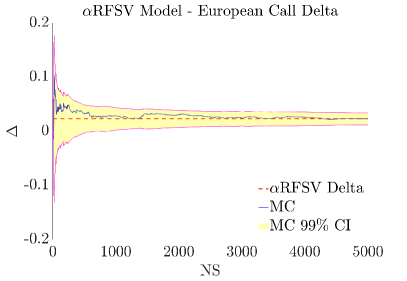
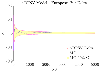
Figure 1: Convergence of the $\alpha$RFSV Delta in the case $H=0.14$.

4.2 Mixed $\alpha$RFSV model

In this section we follow Alòs and León (2021), who considered a mixed fractional Bergomi model in which the volatility process is an arithmetic average of two fractional processes, each with a different Hurst parameter. In particular we consider

$$V_{t}=\frac{1}{2}[V_{t}^{H}+V_{t}^{H^{{}^{\prime}}}],$$ (36)

where $V_{t}^{H}$ and $V_{t}^{H^{{}^{\prime}}}$ are $\alpha$RFSV processes defined by (33) with the Hurst parameters $H<\frac{1}{2}$ and $H^{{}^{\prime}}>\frac{1}{2}$. In this setting, volatility processes $V_{t}^{H}$ and $V_{t}^{H^{{}^{\prime}}}$ represents the short-memory and long-memory factors respectively.

Calculations that we performed in Section 4.1 have to be changed in the following way:

$$D_{s}V_{r}=\frac{\rho}{2}[\xi^{H}V_{r}^{H}K_{H}(r,s)+\xi^{H^{{}^{\prime}}}V_{r}^{H{{}^{\prime}}}K_{H^{{}^{\prime}}}(r,s)]{1\!\!1}_{[0,r]}(s)$$ (37)

and

$$D_{t}D_{s}V_{r}=\frac{\rho}{2}[(\xi^{H})^{2}K_{H}(r,s)K_{H}(r,t)V^{H}_{r}+(\xi^{H^{{}^{\prime}}})^{2}K_{H^{{}^{\prime}}}(r,s)K_{H^{{}^{\prime}}}(r,t)V^{H^{{}^{\prime}}}_{r}]{1\!\!1}_{[0,r]}(s\vee t).$$ (38)

Moreover, we have

$$G(t,T) =V_{t}+\int_{t}^{T}D_{t}V_{r}dW_{r}-\int_{t}^{T}V_{r}D_{t}V_{r}\,\mathrm{d}r$$

$$=\frac{1}{2}[V_{t}^{H}+V_{t}^{H^{{}^{\prime}}}]$$

$$\quad+\frac{\rho}{2}\left(\xi^{H}\int_{t}^{T}V_{r}^{H}K_{H}(r,t)\,\mathrm{d}W_{r}+\xi_{H^{{}^{\prime}}}\int_{t}^{T}V_{r}^{H^{{}^{\prime}}}K_{H^{{}^{\prime}}}(r,t)\,\mathrm{d}W_{r}\right)$$

$$\quad-\frac{\rho}{2}\left(\xi^{H}\int_{t}^{T}(V_{r}^{H})^{2}K_{H}(r,t)\,\mathrm{d}r+\xi^{{H}^{{}^{\prime}}}\int_{t}^{T}(V_{r}^{{H}^{{}^{\prime}}})^{2}K_{H^{{}^{\prime}}}(r,t)\,\mathrm{d}r\right)$$

and

$$\int_{0}^{T}G(t,T)\,\mathrm{d}t =\frac{1}{2}\int_{0}^{T}[V_{t}^{H}+V_{t}^{H^{{}^{\prime}}}]\,\mathrm{d}t$$

$$\quad+\frac{\rho}{2}\left(\xi^{H}\int_{0}^{T}\int_{t}^{T}V_{r}^{H}K_{H}(r,t)\,\mathrm{d}W_{r}\,\mathrm{d}t+\xi_{H^{{}^{\prime}}}\int_{0}^{T}\int_{t}^{T}V_{r}^{H^{{}^{\prime}}}K_{H^{{}^{\prime}}}(r,t)\,\mathrm{d}W_{r}\,\mathrm{d}t\right)$$

$$\quad-\frac{\rho}{2}\left(\xi^{H}\int_{0}^{T}\int_{t}^{T}(V_{r}^{H})^{2}K_{H}(r,t)\,\mathrm{d}rdt+\xi^{{H}^{{}^{\prime}}}\int_{0}^{T}\int_{t}^{T}(V_{r}^{{H}^{{}^{\prime}}})^{2}K_{H^{{}^{\prime}}}(r,s)\,\mathrm{d}rdt\right).$$

Finally

$$D_{s}G(t,T) =D_{s\wedge t}V_{s\vee t}+\int_{s\vee t}^{T}D_{s}D_{t}V_{r}\,\mathrm{d}W_{r}-\int_{s\vee t}^{T}D_{s}V_{r}\cdot D_{t}V_{r}\,\mathrm{d}r-\int_{s\vee t}^{T}V_{r}\cdot D_{s}D_{t}V_{r}\,\mathrm{d}r$$

$$=\frac{\rho}{2}\xi^{H}V_{s\vee t}^{H}K_{H}(s\vee t,s\wedge t)+\frac{1}{2}\xi^{H^{{}^{\prime}}}V_{s\vee t}^{H{{}^{\prime}}}K_{H^{{}^{\prime}}}(s\vee t,s\wedge t)$$

$$\quad+\frac{\rho}{2}\int_{s\vee t}^{T}\left[(\xi^{H})^{2}K_{H}(r,s)K_{H}(r,t)V^{H}_{r}+(\xi^{H^{{}^{\prime}}})^{2}K_{H^{{}^{\prime}}}(r,s)K_{H^{{}^{\prime}}}(r,t)V^{H^{{}^{\prime}}}_{r}\right]\,\mathrm{d}W_{r}$$

$$\quad-\frac{\rho}{4}\int_{s\vee t}^{T}\left[\xi^{H}V_{t}^{H}K_{H}(r,s)+\xi^{H^{{}^{\prime}}}V_{t}^{H{{}^{\prime}}}K_{H^{{}^{\prime}}}(r,s)\right]\cdot\left[\xi^{H}V_{t}^{H}K_{H}(r,t)+\xi^{H^{{}^{\prime}}}V_{r}^{H{{}^{\prime}}}K_{H^{{}^{\prime}}}(r,t)\right]\,\mathrm{d}r$$

$$\quad-\frac{\rho}{4}\int_{s\vee t}^{T}\left[V_{r}^{H}+V_{r}^{H^{{}^{\prime}}}\right]\cdot\left[(\xi^{H})^{2}K_{H}(r,s)K_{H}(r,t)V^{H}_{r}+(\xi^{H^{{}^{\prime}}})^{2}K_{H^{{}^{\prime}}}(r,s)K_{H^{{}^{\prime}}}(r,t)V^{H^{{}^{\prime}}}_{r}\right]\,\mathrm{d}r$$

and

$$\int_{0}^{T}\int_{0}^{T}D_{s}G(t,T)\,\mathrm{d}s\,\mathrm{d}t$$

$$=\frac{\rho}{2}\int_{0}^{T}\int_{0}^{T}\left[\xi^{H}V_{s\vee t}^{H}K_{H}(s\vee t,s\wedge t)+\xi^{H^{{}^{\prime}}}V_{t}^{H{{}^{\prime}}}K_{H^{{}^{\prime}}}(s\vee t,s\wedge t)\right]\,\mathrm{d}s\,\mathrm{d}t$$

$$\quad+\frac{\rho}{2}\int_{0}^{T}\int_{0}^{T}\int_{s\vee t}^{T}\left[(\xi^{H})^{2}K_{H}(r,s)K_{H}(r,t)V^{H}_{r}+(\xi^{H^{{}^{\prime}}})^{2}K_{H^{{}^{\prime}}}(r,s)K_{H^{{}^{\prime}}}(r,t)V^{H^{{}^{\prime}}}_{r}\right]\,\mathrm{d}W_{r}\,\mathrm{d}s\,\mathrm{d}t$$

$$\quad-\frac{\rho}{4}\int_{0}^{T}\int_{0}^{T}\int_{s\vee t}^{T}\left[\xi^{H}V_{t}^{H}K_{H}(r,s)+\xi^{H^{{}^{\prime}}}V_{t}^{H{{}^{\prime}}}K_{H^{{}^{\prime}}}(r,s)\right]\cdot\left[\xi^{H}V_{t}^{H}K_{H}(r,t)+\xi^{H^{{}^{\prime}}}V_{r}^{H{{}^{\prime}}}K_{H^{{}^{\prime}}}(r,t)\right]\,\mathrm{d}r\,\mathrm{d}s\,\mathrm{d}t$$

$$\quad-\frac{\rho}{4}\int_{0}^{T}\int_{0}^{T}\int_{s\vee t}^{T}\left[V_{r}^{H}+V_{r}^{H^{{}^{\prime}}}\right]\cdot\left[(\xi^{H})^{2}K_{H}(r,s)K_{H}(r,t)V^{H}_{r}+(\xi^{H^{{}^{\prime}}})^{2}K_{H^{{}^{\prime}}}(r,s)K_{H^{{}^{\prime}}}(r,t)V^{H^{{}^{\prime}}}_{r}\right]\,\mathrm{d}r\,\mathrm{d}s\,\mathrm{d}t.$$

4.3 Rough Stein-Stein model

Now we assume the volatility $V$ satisfies the equation

$$V_{s}=V_{0}+\int_{0}^{s}\kappa(\theta-V_{u})\,\mathrm{d}u+\nu\int_{0}^{s}K_{H}(s,u)\,\mathrm{d}Z_{u},$$

where $\kappa$, $\theta$ and $\nu$ are positive constants.

In relation with the existence and uniqueness of solution of this equation we refer the reader to Nualart and Ouknine (2002). Being the drift term derivable the Malliavin differentiability of the solution is straightforward.

Then, for $t\leq s$ we have

$$D_{t}V_{s}=\rho\nu K_{H}(s,t)-\kappa\int_{t}^{s}D_{t}V_{u}\,\mathrm{d}u.$$

This is a linear integral equation. Its solution is given by

$$D_{t}V_{s}=\rho\nu K_{H}(s,t)-\kappa\rho\nu\int_{t}^{s}K_{H}(u,t)\mathrm{e}^{-\kappa(s-u)}\,\mathrm{d}u.$$

Being $D_{t}V_{u}$ deterministic, $D_{s}D_{t}V_{u}$ is null. Then, applying Lemma 3.1 we have

$$G(t,T)=V_{t}+\int_{t}^{T}D_{t}V_{u}(\,\mathrm{d}W_{u}-V_{u}\,\mathrm{d}u)$$

and using Lemma 3.2 we have

$$D_{s}G(t,T)=D_{s\wedge t}V_{s\vee t}-\int_{s\vee t}^{T}D_{t}V_{u}D_{s}V_{u}\,\mathrm{d}u.$$

Then,

$$\int_{0}^{T}G(t,T)\,\mathrm{d}t=\int_{0}^{T}V_{t}\,\mathrm{d}t+\rho\nu\int_{0}^{T}\left(\int_{0}^{s}D_{t}V_{s}\,\mathrm{d}t\right)(\,\mathrm{d}W_{s}-V_{s}\,\mathrm{d}s)$$

and

$$\int_{0}^{T}\int_{0}^{T}D_{s}G(t,T)\,\mathrm{d}s\,\mathrm{d}t=\int_{0}^{T}\int_{0}^{T}D_{s\wedge t}V_{s\vee t}\,\mathrm{d}s\,\mathrm{d}t-\int_{0}^{T}\left(\int_{0}^{u}D_{s}V_{u}\,\mathrm{d}s\right)^{2}\,\mathrm{d}u.$$

5 Conclusion

We used Malliavin calculus techniques to obtain formulas for computing Greeks under different rough Volterra stochastic volatility models. In particular we showed that each model is fully characterized by the quantity $G(t,T)$, defined in (20), and by its Malliavin derivative $D_{s}G(t,T)$ (see Lemma 3.2). Calculating the integrals (24) and (25) then leads us directly to all the Greeks formulas listed in Theorem 3.3 and Proposition 3.4. In particular we derived formulas for rough versions of the Stein-Stein, SABR and Bergomi models.

Further research directions may involve other rough volatility models such as some rough Heston variant and also a further numerical analysis of all obtained formulas.

Funding

The work of Josep Vives was partially supported by Spanish grant PID2020-118339GB-100 (2021-2024).

Appendix A Greeks formulas in non-fractional Volterra SV models

In this Appendix we present Greeks formulas for the corresponding non-fractional SV models treated in the present paper. Concretely, for the $\alpha$SV model (Section A.1) and for the Stein-Stein model (Section A.2).

A.1 $\alpha$SV model

Although Merino, Pospíšil, Sobotka, Sottinen, and Vives (2021) introduced the $\alpha$RFSV model directly in the (rough) fractional form, it makes a perfect sense to consider also its non-fractional version called $\alpha$SV model, i.e. the case with $H=1/2$ , that also reduces to known models for particular choice of the parameter $\alpha$. In particular, for $\alpha=1$ we get the Bergomi model (Bergomi, 2016), that in the particular case of $r=0$, coincides with the SABR($\beta=1$) model (Hagan, Kumar, Lesniewski, and Woodward, 2002). For $\alpha=0$ the model is the non-stationary exponential volatility model presented in Gatheral, Jaisson, and Rosenbaum (2018).

Here we introduce a slightly more general model. In this case, we assume the price process satisfies the equation

$$\,\mathrm{d}S_{t}=rS_{t}\,\mathrm{d}t+\sqrt{V_{t}}S_{t}\,\mathrm{d}W_{t},$$ (39)

and the volatility process is

$$V_{t}=V_{0}\exp\left\{\xi Z_{t}-\frac{1}{2}\alpha\xi^{2}t\right\}.$$

Here $V_{0}$ and $\xi$ are positive constants and $\alpha\in[0,1].$

Note that

$$D_{t}V_{s}=\rho\xi V_{s}{1\!\!1}_{[0,s]}(t).$$

Then,

$$G(t,T)=\sqrt{V_{t}}+\frac{\rho\xi}{2}\int_{t}^{T}\sqrt{V_{s}}\,\mathrm{d}W_{s}-\frac{\rho\xi}{2}\int_{t}^{T}V_{s}\,\mathrm{d}s$$

and

$$D_{s}G(t,T)=\frac{\rho\xi}{2}\sqrt{V_{s\vee t}}+\frac{\rho^{2}\xi^{2}}{4}\int_{s\vee t}^{T}\sqrt{V_{u}}\,\mathrm{d}W_{u}-\frac{\rho^{2}\xi^{2}}{2}\int_{s\vee t}^{T}V_{u}\,\mathrm{d}u.$$

A.2 Stein-Stein model

In the Stein and Stein model, see Stein and Stein (1991), we have the price process

$$\,\mathrm{d}S_{t}=rS_{t}\,\mathrm{d}t+V_{t}S_{t}\,\mathrm{d}W_{t},$$ (40)

where $V$ is the volatility process described by the Gaussian Ornstein-Uhlenbeck process

$$\,\mathrm{d}V_{t}=\kappa(\theta-V_{t})\,\mathrm{d}t+\nu\,\mathrm{d}Z_{t}.$$ (41)

Therefore, in this case, $\sigma(x)=x$, $u(x)=\kappa(\theta-x)$ and $v(x)=\nu.$ And first derivatives are $\sigma^{\prime}(x)=1$, $u^{\prime}(x)=-\kappa$ and $v^{\prime}(x)=0.$

Then,

$$D_{t}V_{s}=\rho\nu\mathrm{e}^{-\kappa(s-t)}{1\!\!1}_{[0,s]}(t).$$

And this leads to

$$G(t,T) = V_{t}+\int_{t}^{T}D_{t}V_{s}\,\mathrm{d}W_{s}-\int_{t}^{T}V_{s}D_{t}V_{s}\,\mathrm{d}s$$

$$= V_{t}+\rho\nu\int_{t}^{T}$$

$$e^{-\kappa(s-t)}\,\mathrm{d}W_{s}-\rho\nu\int_{t}^{T}V_{s}\mathrm{e}^{-\kappa(s-t)}\,\mathrm{d}s$$

and

$$D_{s}G(t,T)=\rho\nu\mathrm{e}^{-\kappa(s\vee t-s\wedge t)}-\rho\nu\mathrm{e}^{\kappa(s+t)}\int_{s\vee t}^{T}\mathrm{e}^{-2\kappa u}\,\mathrm{d}u.$$ (42)

References

• Alòs, León, and Vives (2007) Alòs, E., León, J. A., and Vives, J. (2007), On the short-time behavior of the implied volatility for jump-diffusion models with stochastic volatility. Finance Stoch. 11(4), 571–589, ISSN 0949-2984, DOI 10.1007/s00780-007-0049-1, Zbl 1145.91020, MR2335834.
• Alòs, Mazet, and Nualart (2000) Alòs, E., Mazet, O., and Nualart, D. (2000), Stochastic calculus with respect to fractional Brownian motion with Hurst parameter lesser than $\frac{1}{2}$. Stochastic Process. Appl. 86(1), 121–139, ISSN 0304-4149, DOI 10.1016/S0304-4149(99)00089-7, Zbl 1028.60047, MR1741199.
• Alòs and León (2021) Alòs, E. and León, J. A. (2021), An intuitive introduction to fractional and rough volatilities. Mathematics 9(9), 994, ISSN 2227-7390, DOI 10.3390/math9090994.
• Bayer, Friz, and Gatheral (2016) Bayer, C., Friz, P., and Gatheral, J. (2016), Pricing under rough volatility. Quant. Finance 16(6), 887–904, ISSN 1469-7688, DOI 10.1080/14697688.2015.1099717, MR3494612.
• Bennedsen, Lunde, and Pakkanen (2017) Bennedsen, M., Lunde, A., and Pakkanen, M. S. (2017), Hybrid scheme for Brownian semistationary processes. Finance Stoch. 21(4), 931–965, ISSN 0949-2984, DOI 10.1007/s00780-017-0335-5, Zbl 1385.65010, MR3723378.
• Bergomi (2016) Bergomi, L. (2016), Stochastic Volatility Modeling. Chapman and Hall/CRC Financial Mathematics Series, Boca Raton: Chapman and Hall/CRC, ISBN 978-1-4822-4407-6, Zbl 1329.91003, MR3445286.
• Black and Scholes (1973) Black, F. and Scholes, M. (1973), The pricing of options and corporate liabilities. J. Polit. Econ. 81(3), 637–654, ISSN 0022-3808, DOI 10.1086/260062, Zbl 1092.91524, MR3363443.
• Cont (2001) Cont, R. (2001), Empirical properties of asset returns: stylized facts and statistical issues. Quant. Finance 1(2), 223–236, ISSN 1469-7688, DOI 10.1080/713665670, Zbl 1408.62174.
• Davis and Johansson (2006) Davis, M. H. A. and Johansson, M. P. (2006), Malliavin Monte Carlo Greeks for jump diffusions. Stochastic Process. Appl. 116(1), 101–129, ISSN 0304-4149, DOI 10.1016/j.spa.2005.08.002, Zbl 1081.60040, MR2186841.
• Di Nunno, Kubilius, Mishura, and Yurchenko-Tytarenko (2023) Di Nunno, G., Kubilius, K., Mishura, Y., and Yurchenko-Tytarenko, A. (2023), From constant to rough: A survey of continuous volatility modeling, available at arXiv: https://arxiv.org/abs/2309.01033.
• Eberlein, Eddahbi, and Lalaoui Ben Cherif (2016) Eberlein, E., Eddahbi, M., and Lalaoui Ben Cherif, S. M. (2016), Computation of Greeks in LIBOR models driven by time-inhomogeneous Lévy processes. Appl. Math. Finance 23(3), 236–260, ISSN 1350-486X, DOI 10.1080/1350486X.2016.1243013, Zbl 1396.91779, MR3572024.
• Eddahbi, Lalaoui Ben Cherif, and Nasroallah (2015) Eddahbi, M., Lalaoui Ben Cherif, S. M., and Nasroallah, A. (2015), Computation of Greeks for jump-diffusion models. Int. J. Theor. Appl. Finance 18(6), 1550039, 30, ISSN 0219-0249, DOI 10.1142/S0219024915500399, Zbl 1337.91094, MR3397252.
• El-Khatib (2009) El-Khatib, Y. (2009), Computations of Greeks in stochastic volatility models via the Malliavin calculus, DOI 10.48550/arXiv.0904.3247, available at arXiv: https://arxiv.org/abs/0904.3247.
• Fournié, Lasry, Lebuchoux, and Lions (2001) Fournié, E., Lasry, J.-M., Lebuchoux, J., and Lions, P.-L. (2001), Applications of Malliavin calculus to Monte Carlo methods in finance II. Finance Stoch. 5(2), 201–236, ISSN 0949-2984, DOI 10.1007/PL00013529, Zbl 0973.60061, MR1841717.
• Fournié, Lasry, Lebuchoux, Lions, and Touzi (1999) Fournié, E., Lasry, J.-M., Lebuchoux, J., Lions, P.-L., and Touzi, N. (1999), Applications of Malliavin calculus to Monte Carlo methods in finance. Finance Stoch. 3(4), 391–412, ISSN 0949-2984, DOI 10.1007/s007800050068, Zbl 0947.60066, MR1842285.
• Gatheral, Jaisson, and Rosenbaum (2018) Gatheral, J., Jaisson, T., and Rosenbaum, M. (2018), Volatility is rough. Quant. Finance 18(6), 933–949, ISSN 1469-7688, DOI 10.1080/14697688.2017.1393551, Zbl 1400.91590, MR3805308.
• Hagan, Kumar, Lesniewski, and Woodward (2002) Hagan, P. S., Kumar, D., Lesniewski, A. S., and Woodward, D. E. (2002), Managing smile risk. Wilmott Magazine 2002(January), 84–108.
• Heston (1993) Heston, S. L. (1993), A closed-form solution for options with stochastic volatility with applications to bond and currency options. Rev. Financ. Stud. 6(2), 327–343, ISSN 0893-9454, DOI 10.1093/rfs/6.2.327, Zbl 1384.35131, MR3929676.
• Hull and White (1987) Hull, J. C. and White, A. D. (1987), The pricing of options on assets with stochastic volatilities. J. Finance 42(2), 281–300, ISSN 1540-6261, DOI 10.1111/j.1540-6261.1987.tb02568.x.
• Khedher (2012) Khedher, A. (2012), Computation of the delta in multidimensional jump-diffusion setting with applications to stochastic volatility models. Stoch. Anal. Appl. 30(3), 403–425, ISSN 0736-2994, DOI 10.1080/07362994.2012.668440, Zbl 1242.91188, MR2916862.
• Matas and Pospíšil (2021) Matas, J. and Pospíšil, J. (2021), Robustness and sensitivity analyses for rough Volterra stochastic volatility models, DOI 10.48550/arXiv.2107.12462, available at arXiv: https://arxiv.org/abs/2107.12462.
• Merino, Pospíšil, Sobotka, Sottinen, and Vives (2021) Merino, R., Pospíšil, J., Sobotka, T., Sottinen, T., and Vives, J. (2021), Decomposition formula for rough Volterra stochastic volatility models. Int. J. Theor. Appl. Finance 24(2), 2150008, ISSN 0219-0249, DOI 10.1142/S0219024921500084, Zbl 1466.91350, MR4257140.
• Mhlanga (2015) Mhlanga, F. J. (2015), Calculations of Greeks for jump diffusion processes. Mediterr. J. Math. 12(3), 1141–1160, ISSN 1660-5446, DOI 10.1007/s00009-014-0459-1, Zbl 1321.60168, MR3376837.
• Mishura (2019) Mishura, Y. (2019), Fractional stochastic volatility: F-Ornstein–Uhlenbeck and F-CIR processes. In Computer Data Analysis and Modeling: Stochastics and Data Science : Proc. of the Twelfth Intern. Conf., Minsk, Sept. 18-22, 2019., pp. 94–101, Minsk: BSU, ISBN 978-985-566-811-5.
• Montero and Kohatsu-Higa (2003) Montero, M. and Kohatsu-Higa, A. (2003), Malliavin calculus applied to finance. Phys. A 320(1-4), 548–570, ISSN 0378-4371, DOI 10.1016/S0378-4371(02)01531-5, Zbl 1010.91046, MR1963722.
• Nualart (2006) Nualart, D. (2006), The Malliavin calculus and related topics. Probab. Appl., Berlin: Springer-Verlag, 2nd edn., ISBN 3-540-28328-5/hbk; 978-3-642-06651-1/pbk; 3-540-28329-3/ebook, DOI 10.1007/3-540-28329-3, Zbl 1099.60003, MR2200233.
• Nualart and Nualart (2018) Nualart, D. and Nualart, E. (2018), Introduction to Malliavin calculus, vol. 9 of Institute of Mathematical Statistics Textbooks. Cambridge University Press, Cambridge, ISBN 978-1-107-61198-6; 978-1-107-03912-4, DOI 10.1017/9781139856485, Zbl 06968586, MR3838464, URL https://doi.org/10.1017/9781139856485.
• Nualart and Ouknine (2002) Nualart, D. and Ouknine, Y. (2002), Regularization of differential equations by fractional noise. Stochastic Processes Appl. 102(1), 103–116, ISSN 0304-4149, DOI 10.1016/S0304-4149(02)00155-2, Zbl 1075.60536, MR1934157.
• Petrou (2008) Petrou, E. (2008), Malliavin calculus in Lévy spaces and applications to finance. Electron. J. Probab. 13(27), 852–879, ISSN 1083-6489/e, DOI 10.1214/EJP.v13-502, Zbl 1193.60075, MR2399298.
• Stein and Stein (1991) Stein, E. M. and Stein, J. C. (1991), Stock price distributions with stochastic volatility: An analytic approach. Rev. Financ. Stud. 4(4), 727–752, ISSN 0893-9454, DOI 10.1093/rfs/4.4.727, Zbl 06857133.
• Thao (2006) Thao, T. H. (2006), An approximate approach to fractional analysis for finance. Nonlinear Anal. Real World Appl. 7(1), 124–132, ISSN 1468-1218, DOI 10.1016/j.nonrwa.2004.08.012, Zbl 1104.60033, MR2183802.
• Yamada (2017) Yamada, T. (2017), A weak approximation with Malliavin weights for local stochastic volatility model. Int. J. Financ. Eng. 4(1), 1750002, ISSN 2424-7863, DOI 10.1142/S2424786317500025, MR3632288.
• Yilmaz (2018) Yilmaz, B. (2018), Computation of option greeks under hybrid stochastic volatility models via Malliavin calculus. Mod. Stoch. Theory Appl. 5(2), 145–165, ISSN 2351-6046, DOI 10.15559/18-vmsta100, Zbl 1390.60198, MR3813089.
• Yolcu-Okur, Sayer, Yilmaz, and Inkaya (2018) Yolcu-Okur, Y., Sayer, T., Yilmaz, B., and Inkaya, B. A. (2018), Computation of the delta of European options under stochastic volatility models. Comput. Manag. Sci. 15(2), 213–237, ISSN 1619-697X, DOI 10.1007/s10287-018-0316-y, Zbl 1417.91518, MR3817795.