A Framework for Solving Parabolic Partial Differential Equations on Discrete Domains

Abstract.

We introduce a framework for solving a class of parabolic partial differential equations on triangle mesh surfaces, including the Hamilton-Jacobi equation and the Fokker-Planck equation. PDE in this class often have nonlinear or stiff terms that cannot be resolved with standard methods on curved triangle meshes. To address this challenge, we leverage a splitting integrator combined with a convex optimization step to solve these PDE. Our machinery can be used to compute entropic approximation of optimal transport distances on geometric domains, overcoming the numerical limitations of the state-of-the-art method. In addition, we demonstrate the versatility of our method on a number of linear and nonlinear PDE that appear in diffusion and front propagation tasks in geometry processing.

Figure 1. We show the time evolution of the Fokker-Planck equation under a certain flow on the discrete sphere with $81{,}920$ triangle faces and $40{,}962$ vertices, obtained using our framework. Our method can be used for any equation in a class of second-order parabolic PDE on triangle mesh surfaces.

1. Introduction

The analysis of partial differential equations (PDE) is a ubiquitous technique in computer graphics, geometry processing, and adjacent fields. In particular, parabolic PDE describe a wide variety of phenomena. For example, instances of the Hamilton-Jacobi equation model the time evolution of front propagation and the evolution of functions undergoing nonlinear diffusion. The Fokker-Planck equation describes the evolution of density functions driven by stochastic processes. Each of these equations has a long history as a means to study various problems in computer graphics, including modeling flames and fire (Nguyen et al., 2002), stochastic heat kernel estimation (Aumentado-Armstrong and Siddiqi, 2017), medial axis detection (Du and Qin, 2004), and texture synthesis (Witkin and Kass, 1991). Hence, methods to solve this class of PDE over geometric domains are central in geometry processing.

Myriad numerical algorithms have been proposed for solving PDE in geometry processing. Unfortunately, the most popular algorithms are unsuitable for important regimes, such as capturing infinitesimal or nonlinear phenomena. An interesting example involves the convolutional Wasserstein distance method for barycenter computation (Solomon et al., 2015). The aforementioned method is built on tiny amounts of diffusion, but relies on heuristics for choosing diffusion times. If the diffusion time step is too small, then the method leads to numerical inaccuracies, and if the step is too large, then the method results in approximations that quantitatively appear wrong. Another example involves nonlinear PDE used to describe certain types of flows. In this case, the challenge is that explicit integrators used for these PDE require time step restrictions to avoid numerical instability, and implicit integration schemes are not equivalent to solving a single linear system of equations, turning out to be too expensive.

To address these challenges, we propose a framework leveraging a splitting integration strategy and an appropriate spatial discretization to solve parabolic PDE over discrete geometric domains. The splitting allows us to leverage the implicit integration of a well-known PDE, the heat equation, and use a convex relaxation to deal with the challenging piece of the parabolic PDE. Empirically, our method overcomes limitations presented by state-of-the-art methods in geometry processing. We apply our framework to difficult parabolic PDE: log-domain heat diffusion, the nonlinear $G$-equation, and the Fokker-Planck equation, all of which we solve efficiently on a variety of domains and time steps.

Contributions.

Our main contributions are:

• A numerical framework to solve linear and nonlinear parabolic PDE on curved triangle meshes with efficiency matching that of conventional methods in geometry processing.

• A log-domain diffusion algorithm that overcomes known limitations of geometry processing methods relying on tiny amounts of diffusion, demonstrated on optimal transport tasks.

• An application of our framework to numerical integration of the $G$-equation, which can be used as foundational work in graphics pipelines for the simulation of fire and flames.

2. Related Work

2.1. PDE-driven geometry processing

PDE are a fundamental component of many geometry processing algorithms. PDE-based approaches have been used for surface fairing (Desbrun et al., 1999; Bobenko and Schröder, 2005), surface reconstruction (Duan et al., 2004; Xu et al., 2006), and physics-based simulation (Chen et al., 2013; O’Brien et al., 2002), to cite a few examples. Hence, there has been a considerable amount of work focused on developing accurate and robust PDE solvers. The most popular PDE-based methods, however, such as the “heat method” for geodesic distance approximations (Crane et al., 2013), are concerned with solving linear PDE problems.

2.2. Second-order Parabolic PDE

Second-order parabolic PDE comprise a general extension of the heat equation. The solutions to PDE in this class are in some ways related to the solutions of the heat equation; these equations appear in similiar applications where the object of interest is the density of a quantity on a domain, evolving forward in time. While the heat equation is a well-studied PDE with a wide array of tools available to solve it on discrete domains, second-order parabolic PDE in general are more challenging, in particular in the presence of additional terms that add nonlinearity or chaotic behaviour.

The typical strategy for spatial discretization of second-order parabolic PDE are Garlekin methods (Evans, 2010). Common numerical integration techniques are finite difference schemes, including forward Euler, explicit Runge-Kutta formulas, backward Euler, and the Crank-Nicolson method. Still, many PDE in this family cannot be efficiently solved on triangle meshes with these discretization methods. Some of the difficulties that arise include the following: the strong stiffness of certain equations in this family is not suitable for methods such as Runge-Kutta (Sommeijer et al., 1998); and equations such as the Hamilton-Jacobi do not have a conservative form, making it difficult to write out fluxes for discontinuous Garlekin methods adapted to irregular domains (Yan and Osher, 2011).

2.2.1. Heat diffusion and entropy-regularized optimal transport

The entropy-regularized approximation of transport distances provides a method for solving various optimal transportation problems by realizing them as optimization problems in the space of probability measures equipped with the Kullback-Leibler (KL) divergence. We refer the reader to (Villani, 2003) for a complete introduction to the optimal transportation problem, which roughly seeks to transport all the mass from a source distribution to a target distribution with minimal cost. (Cuturi, 2013; Benamou et al., 2015) link entropy-regularized transport to minimizing a KL divergence.

Cuturi (2013) proposed a fast computational method to compute transport distances using entropic regularization based on the Sinkhorn algorithm. Solomon et al. (2015) extended this work by showing that the kernel in the Sinkhorn algorithm for the 2-Wasserstein distance can be approximated with the heat kernel, which can be computed using PDE solution techniques over geometric domains. Huguet et al. (2023) presents a similar attempt at improving Sinkhorn-based methods on discrete manifolds. This perspective is also echoed in Schrödinger bridge formulations of transport, whose static form includes an identical substitution of the heat kernel (Léonard, 2014).

We leverage this approximation with the heat kernel over geometric domains, and show in §§7.1–7.2 that the numerical challenges arising for small entropy coefficients can be overcome by using our framework to solve a certain second-order parabolic nonlinear PDE.

Figure 2. Wasserstein barycenters (green) between two distributions on the unit line (grey) with $1{,}000$ elements for varying pairs of weights. Our method obtains these barycenters for a tiny amount of entropy, i.e., $\gamma=10^{-7}$, whereas the method in Solomon et al. (2015) fails.

Description

2.2.2. $G$-equation

The $G$-equation is a level-set Hamilton-Jacobi equation introduced by F.A. Williams in (Williams, 1985) to model turbulent-flame propagation in combustion theory. While some finite difference schemes have succeeded in solving various cases of the $G$-equation on regular grids (Liu et al., 2013; Gu et al., 2021). Several challenges arise in the curved triangle mesh setting: for certain values of flow intensity, the constraint on time step—given by the Courant–Friedrichs–Lewy (CFL) condition—is quite restrictive on explicit methods; and the nonlinearity of the equation yields an open problem for implicit methods.

While the $G$-equation is well-known in computational fluid dynamics (CFD) (Nielsen et al., 2022), it was brought to the computer graphics community as the “thin-flame model” to simulate flame and fire in (Nguyen et al., 2002). This work was later extended to model a wider variety of combustion phenomena in graphics, e.g., see (Hong et al., 2007). The time integration implemented in these graphics pipelines are based on the foundational scheme introduced by Osher and Sethian (1988), which deals with the aforementioned limitations, in particular, time step restrictions due to a CFL condition.

As we will show in §7.3, our framework achieves better numerical stability than this standard scheme for regimes in violation of its CFL condition, and matches numerical results for regimes within its CFL condition, where the standard scheme provides a reasonable approximation of the exact solution.

2.2.3. Fokker–Planck equation

The Fokker-Planck equation is a linear parabolic partial differential equation describing the time evolution of the probability density function of a process driven by a stochastic differential equation (SDE). Processes driven by SDE and the Fokker-Planck equation appear in applications in computer vision and image processing (Smolka and Wojciechowski, 1997; Leatham et al., 2022). In the context of computer graphics and geometry processing, the Fokker-Planck equation and its variants have been used for texture synthesis based on nonlinear interactions (Witkin and Kass, 1991) and stochastic kernel estimation (Aumentado-Armstrong and Siddiqi, 2017).

We show that our framework can be used to solve the Fokker-Planck equation directly on curved triangle meshes, in contrast to using its SDE formulation. In this way, our work lays the foundation for a new approach to using stochastic differential equations in traditional geometry processing.

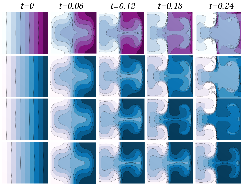
Figure 3. Level-sets of the $G$-equation under cellular flow obtained via our method with varying values of viscosity: $\varepsilon=0,10^{-4},10^{-3},$ and $10^{-2}$ (from top to bottom, respectively). See Figure 4 for an illustration of cellular flow.

Description

2.3. Convex Optimization for Regularized Geodesics

Perhaps the closest related work to our paper is  (Edelstein et al., 2023), which proposes a convex optimization technique for extracting regularized geodesic distances on triangle meshes. Their paper generalizes the PDE-based results in (Belyaev and Fayolle, 2020, 2015) from estimation of distance-like functions to general regularizers under some mild conditions. This optimization approach is based on the equivalence found between the solution of an eikonal type equation, i.e., a stationary first-order PDE dependent only on the gradient of a variable function, and the solution to a volume maximization problem. The equivalence is a consequence of mathematical results on the study of maximal viscosity subsolutions of eikonal type equations first introduced by (Ishii, 1987). In our case, we handle the problem of more general evolutionary Hamilton-Jacobi equations with Hamiltonians depending on the variable function rather than just its gradient.

3. Mathematical Preliminaries

3.1. General Preliminaries

Let $\mathcal{M}\subset\mathbb{R}^{3}$ be a surface embedded in $\mathbb{R}^{3}$, possibly with boundary $\partial\mathcal{M}$; we will use $\hat{n}(x)$ to denote the unit normal to the boundary $\partial\mathcal{M}$ at $x\in\partial\mathcal{M}$. Take $\nabla$ to be the gradient operator and $\Delta$ to be the Laplacian operator, with the convention that $\Delta$ has nonnegative eigenvalues. We refer the reader to (Jost, 2011) for a general introduction to Laplacian operators, which roughly map functions to their total second derivative pointwise.

Let $q$ denote $\nabla u(x)$. In this paper we consider evolutionary, that is, time-varying, second-order parabolic PDE of the following form:

(1) $$\frac{\partial u}{\partial t}=-\varepsilon\Delta u+H(x,q,u),$$

where $\varepsilon\geq 0$ and $u(x,t)\colon\mathcal{M}\times[0,\infty)\to\mathbb{R}$ is an unknown variable function. If $\varepsilon>0$, then $u$ is guaranteed to be twice differentiable on $\mathcal{M}$. The function $H(x,q,u)\colon T^{*}\mathcal{M}\times\mathbb{R}\to\mathbb{R}$ is the Hamiltonian on $T^{*}\mathcal{M}$ of

(2) $$\frac{\partial u}{\partial t}=H(x,q,u),$$

which is known as the Hamilton-Jacobi equation (Evans, 2010). The parameter $\varepsilon$ in (1) is called the viscosity parameter and, as $\varepsilon\to 0$, the function $u$ converges to a solution of (2) (Fleming and Souganidis, 1989).

We tackle the Cauchy problem for (1), that is, with a prescribed initial condition $u(x,0)=u_{0}(x)$, where $u_{0}\colon\mathcal{M}\to\mathbb{R}$ is some scalar function, and boundary conditions determining the behavior of $u(x,t)$ at $x\in\partial\mathcal{M}$. Two common choices for boundary conditions are Dirichlet conditions, which prescribe the values of $u(x,t)$ for all $(x,t)\in\partial\mathcal{M}\times(0,\infty)$, and Neumann conditions, which specify $\nabla u(x,t)\cdot\hat{n}(x)\equiv 0$ for all $x\in\partial\mathcal{M}$.

3.2. Example PDE

Our framework arose in our study of functions $u(x,t)$ satisfying the following PDE:

(3) $$\frac{\partial u}{\partial t}=-\Delta u+\|\nabla u\|_{2}^{2}.$$

This PDE will be referred to in this paper as the “nonlinear diffusion” equation (see §3.2.1). Its name originates from the nonlinear nature of the PDE and its relationship with heat diffusion shown in the proposition below.

Proposition 3.1.

Suppose $v(x,t)$ is such that $v(x,t)>0$ for all $(x,t)\in\mathcal{M}\times[0,\infty)$ and $v$ satisfies the heat equation:

(4) $$\frac{\partial v}{\partial t}=-\Delta v.$$

Define $u(x,t):=\log v(x,t)$. Then, $u(x,t)$ satisfies (3). Moreover, if $v$ satisfies Dirichlet or Neumann boundary conditions, then $u$ satisfies the same boundary conditions up to applying $\log$. In sum, $u$ satisfies the boundary conditions satisfied by $v$ up to applying $\log$.

Proof.

Let $u=\log v$, then this is a straightforward application of the chain rule:

$$\begin{array}[]{rcl}\nicefrac{{\partial u}}{{\partial t}}&=&-\Delta u+\|\nabla u\|_{2}^{2}\\ \implies(\nicefrac{{1}}{{v}})(\nicefrac{{\partial v}}{{\partial t}})&=&-\nabla\cdot\Big{(}\frac{1}{v}\nabla v\Big{)}+\frac{1}{v}\|\nabla v\|_{2}^{2}\\ &=&\frac{1}{v^{2}}(\nabla v\cdot\nabla v)-\frac{1}{v}\Delta v+\frac{1}{v}\|\nabla v\|_{2}^{2}\\ \implies\nicefrac{{\partial v}}{{\partial t}}&=&-\Delta v\end{array}$$

∎

Remark 0.

Proposition 3.1 only applies to strictly positive functions $v(x,t)$; by the maximum principle, it is sufficient to check $v(x,0)>0$ to guarantee this condition for all $t\in[0,\infty)$. Also, $u$ is a supersolution to the heat equation since clearly $\nicefrac{{\partial u}}{{\partial t}}\geq-\Delta u$.

The overarching theme of this paper is that the same numerical procedure that we developed to solve (3) can be generalized to handle other parabolic problems of the form (1) given certain continuity and convexity assumptions on $H$ and $u$. In particular, we assume the following:

• The function $H(x,q,u)$ is continuous on $T^{*}\mathcal{M}\times\mathbb{R}$,

• for any pair $(x,u)\in\mathcal{M}\times\mathbb{R}$, $H(x,q,u)$ is convex on $T_{x}^{*}\mathcal{M}$,

• $|H(x,q,a)-H(x,q,b)|\leq L|a-b|$ for any $(x,q)\in T^{*}\mathcal{M}$ and $a,b\in\mathbb{R}$, where $L$ is a Lipschitz constant,

• $\forall R>0$, $\exists K>0$ such that $H(x,q,u)>R$ if $|u|\leq R$ and $|q|\geq K$.

In this paper, we consider three choices of the function $H=H(x,q,u)$:

3.2.1. Nonlinear diffusion

First, motivated by equation (3), we consider $H(x,q,u)=\|q\|_{2}^{2}$. In §§7.1–7.2, we will show that the nonlinear diffusion equation together with Proposition 3.1 play a key role in overcoming the limitations faced by methods relying on small amounts of diffusion to compute entropy regularized transport distances on discrete domains.

Here, we verify assumptions (A1)–(A4) are fufilled: (A1) and (A2) follow from the continuity and convexity of $L_{2}$ norms; (A3) is an empty condition in this case since $H$ does not depend on $u$; (A4) can be obtained by letting $|q|>\sqrt{R}$. These assumptions can be verified straightforwardly for remaining example PDE by the interested reader.

3.2.2. G-equation

Second, let $\Phi\colon\mathcal{M}\to\mathbb{R}^{3}$ be a vector field, we consider $H(x,q,u)=-\Phi(x)\cdot q+\|q\|_{2}$, which corresponds to the $G$-equation (see §2.2.2):

(5) $$\frac{\partial u}{\partial t}=-\Phi(x)\cdot\nabla u+\|\nabla u\|_{2}-\varepsilon\Delta u.$$

For $\varepsilon>0$, equation (5) is known as the viscous $G$-equation, and when $\varepsilon=0$, it is known as the inviscid $G$-equation.

3.2.3. Fokker-Planck equation

Finally, we consider $H(x,p,q)=u\nabla\Phi(x)+\Phi(x)q$, which corresponds to the Fokker-Planck equation (see §2.2.3):

(6) $$\frac{\partial u}{\partial t}=u\nabla\cdot\Phi(x)+\Phi(x)\cdot\nabla u-\varepsilon\Delta u.$$

Here $u$ is the density function of the trajectories of the following SDE:

(7) $$\mathrm{d}x=-\nabla\cdot\Phi(x)\mathrm{d}t+\sqrt{2\varepsilon}\;\mathrm{d}W,$$

where $W$ is a Wiener process. We refer the reader to (Medved et al., 2020) for a review on the relationship between equations (6)–(7). The vector field $\Phi$ is typically known as the drift vector and $\varepsilon$ as the diffusion coefficient, but we will call the latter the viscosity parameter for consistency throughout this paper.

Figure 4. Three typical examples of vector fields $\Phi$ used when evolving second-order parabolic PDE that involve terms with vector fields.

Description

3.3. Viscosity Solutions

We introduce a few definitions from (Crandall and Lions, 1983) in the study of weak solutions to Hamilton-Jacobi equations. These definitions will be necessary in the proofs presented in section §4.1.3, and we give them in terms of the Cauchy problem presented in (Hitoshi Ishii and Yan, 2022). We refer the reader to (Crandall et al., 1992) for a complete introduction to the theory of viscosity solutions and their applications to PDE.

Definition 3.2 (Viscosity subsolutions, and resp., supersolutions).

Let $V$ be an open subset in the manifold $\mathcal{M}$. A function $u\colon V\to\mathbb{R}$ is a viscosity subsolution (respectively, supersolution) of $\frac{\partial u}{\partial t}+H(x,q,u)=0$ if for every $C^{1}$ function $\varphi\colon V\to\mathbb{R}$ and every point $x\in V$ such that $u-\varphi$ has a local maximum (respectively, minimum) at $x$, we have $\frac{\partial\varphi}{\partial t}+H(x,\nabla\varphi,\varphi)\leq 0$ (respectively, $\frac{\partial\varphi}{\partial t}+H(x,\nabla\varphi,\varphi)\geq 0$).

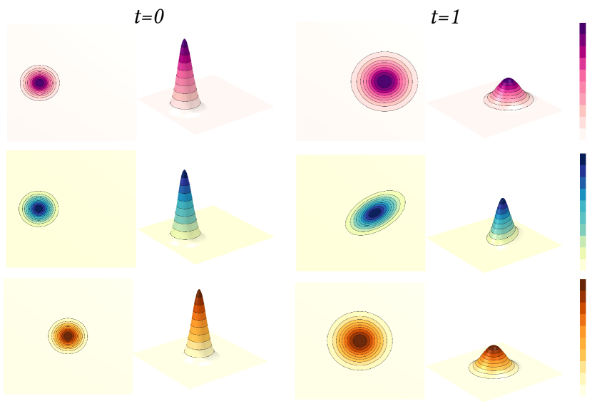
Figure 5. Time evolution of the Fokker-Planck equation (6) on a $100\times 100$ triangle grid, obtained using our method, under constant drift (top), shear flow (middle), and no drift (bottom). See Figure 4 for an illustration of constant drift and shear flow.

Description

Definition 3.3 (Viscosity solution).

A function $u\colon V\to\mathbb{R}$ is a viscosity solution of $\frac{\partial u}{\partial t}+H(x,q,u)=0$ if it is both a subsolution and a supersolution.

We note that the above definitions do not assume the function $u$ to be continuous. In fact, the necessity for such definitions arose in the study of problems without continuous solutions. As stated in §3.1, the functions we study are twice differentiable if $\varepsilon>0$ and hence the following theorem is useful:

Theorem 3.4 (Continuously differentiable viscosity solution).

A $C^{1}$ function $u\colon V\to\mathbb{R}$ is a viscosity solution if and only if it is a classical solution.

Hence, while we might still use the term viscosity solution throu- ghout the paper, when referring to the problem in (2) with $\varepsilon>0$, a viscosity solution is equivalent to a solution in the classical sense.

Figure 6. A two dimensional illustration of a viscosity supersolution $\varphi$.

A visual representation of a viscosity supersolution $\varphi$ in 2D.

4. Method

Let $\Omega=(V,E,F)$ be a triangle mesh with vertices $V\subset\mathbb{R}^{3}$, edges $E\subseteq V\times V$, and triangular faces $F\subset V\times V\times V$. In this section, we develop a general approach to approximating solutions to equations of the form (1) on triangle meshes, given $u(x,0)$ discretized on $(V,F)$ using one value per vertex, $u_{0}\in\mathbb{R}^{|V|}$.

In geometry processing, the most common discretization of the PDE on triangle meshes uses the finite element method (FEM). Following (Botsch et al., 2010), take $L\in\mathbb{R}^{|V|\times|V|}$ to be the cotangent Laplacian matrix associated to our mesh (with appropriate boundary conditions), and take $M\in\mathbb{R}^{|V|\times|V|}$ to be the diagonal matrix of Voronoi cell areas. Also, take $G\in\mathbb{R}^{3|F|\times|V|}$ to be the matrix mapping vertex scalar values to per face gradients. In our time discretization strategy, we will denote the time step size by $h$.

In what follows, we first describe our method for time integration, and then we define a spatio-dicretization strategy suitable to the different terms associated with PDE of the form in (1).

4.1. Time Integration

We now give a brief overview of classical time integration approaches and outline a method to address the challenges faced by classical approaches when solving second-order parabolic PDE.

4.1.1. Classical approaches

Two typical means of solving PDE in time are explicit time integration, such as the forward Euler method, and implicit integration, such as the backward Euler method. Forward Euler often imposes a strict restriction (upper bound) on $h$ for stability. Runge–Kutta and other variations of this integrator can improve stability and accuracy of forward Euler integration, but almost all require that we take many small steps ($h\ll 1$) to avoid introducing instability. Backward Euler is unconditionally stable and first-order accurate in $h$, which often suffices for small $h>0$. If the PDE contains a nonlinear term, however, backward Euler and related implicit integration schemes are no longer equivalent to solving a single linear system of equations; in this case, implicit integration leads to a nonlinear root-finding problem.

4.1.2. Strang splitting

We would like to leverage the effectiveness of implicit integration for the simplest version of (1) where $H=0$, but without having to solve a nonlinear system of equations. To this end, we propose using Strang–Marchuk splitting (also known

as leapfrog or Störmer–Verlet integration), originally proposed in (Strang, 1968; Marchuk, 1988). Generically, operator splitting methods solve differential equations $\nicefrac{{dx}}{{dt}}=f(x)+g(x)$ by alternating steps in which the terms $f$ and $g$ on the right-hand side are treated individually. This splitting scheme is justified by the Lie–Trotter–Kato formula (Trotter, 1959; Kato, 1974). In our case, we choose a splitting so that one piece of the splitting resembles solving the heat equation and the other benefits from the solution techniques along the lines of those introduced by Belyaev and Fayolle (2020) (later extended by Edelstein et al. (2023)).

In particular, suppose $u_{n-1}\in\mathbb{R}^{|V|}$ is our estimate of $u$ at time $h(n-1)$. We estimate $u_{n}$ via the following three steps:

1. First, apply half a time step of implicit heat diffusion, approximating the solution to $\nicefrac{{\partial u}}{{\partial t}}=-\varepsilon\Delta u$ at $t=h(n-1)+\nicefrac{{h}}{{2}}$:

   (8) $$u_{n}^{(1)}=\left(M+h\frac{\varepsilon L}{2}\right)^{-1}Mu_{n-1}.$$

2. Next, apply a full time step approximating the solution to $\nicefrac{{\partial u}}{{\partial t}}=H(x,u,\nabla u)$, as detailed in §4.1.3, to obtain $u_{n}^{(2)}\in\mathbb{R}^{|V|}$.

3. Finally, apply a second half-step of implicit heat diffusion:

   (9) $$u_{n}=\left(M+h\frac{\varepsilon L}{2}\right)^{-1}Mu_{n}^{(2)}.$$

Note that (8) and (9) solve the same linear system with different right-hand sides, allowing us to pre-factor the matrix $M+\nicefrac{{h\varepsilon L}}{{2}}$ if we plan to apply our operator more than once. It is also worth noting that possible time step size limitations in Strang splitting are only imposed by the method chosen to solve each subproblem. The backward Euler substep is unconditionally stable and the convex optimization substep, which is outlined next, enjoys similar stability to implicit methods. Analytically, Strang splitting has convergence of second order (Strang, 1968).

There are different splitting schemes that one could choose when treating different kinds of PDE. We considered accuracy in choosing an suitable splitting scheme for our case. The Lie-Trotter scheme, for instance, is first-order and can provide crude results for nonlinear problems (Strang, 1968). Strang splitting is second-order, i.e., $\mathcal{O}(h^{2})$ given a time step $h$. The nonlinearity in various second-order parabolic PDE makes Strang a preferable choice.

4.1.3. Strang-Marchuk splitting, step II

We use convex optimization to take a time step of the first-order equation $\nicefrac{{\partial u}}{{\partial t}}=H(x,u,\nabla u)$, including the case where this is a nonlinear first-order problem. In this section, we describe an implicit integrator leveraging the fact that $H(x,p,q)$ is jointly convex in its arguments $(p,q)$.

In this step, our goal is to obtain $u_{n}^{(2)}$ by integrating the first-order equation for time $h$ starting at function $u_{n}^{(1)}$. The simplest implicit integration strategy is backward Euler integration, which would solve the following root-finding problem:

(10) $$\frac{u_{n}^{(2)}-u_{n}^{(1)}}{h}=H(x,u_{n}^{(2)},\nabla u_{n}^{(2)}).$$

Here, we will assume the $u_{n}^{(i)}$ are functions on the surface $\mathcal{M}$, but an identical formulation will apply after spatial discretization in §4.2. This problem is nonlinear whenever $H$ is nonlinear, making it difficult to solve.

Instead, we observe that relaxing the equality in (10) to an inequality leads to a convex constraint on the unknown function $u_{n}^{(2)}$. Taking inspiration from Edelstein et al. (2023), we arrive at the following optimization problem to advance forward in time:

(11) $$u_{n}^{(2)}=\left\{\begin{array}[]{rl}\arg\min_{u}&\int_{\mathcal{M}}u(x)\,\mathrm{dVol}(x)\\ \mathrm{subject\;to}&H(x,u,\nabla u)-\frac{1}{h}(u-u_{n}^{(1)})\leq 0\\ &\qquad\mathrm{\;for\;all\;}x\in\mathcal{M}.\end{array}\right.$$

Notice that the constraint in (11) yields a supersolution of the implicit problem (10). Moreover, formulation (11) is a convex problem for $u$ since it has a linear objective and a pointwise convex constraint.

The intuitive argument for the equivalence between solutions to eikonal type equations and solutions to a convex optimization problem given in (Belyaev and Fayolle, 2020), and later used by (Edelstein et al., 2023) is not sufficient to obtain the well-posedness of (11) and its equivalence to (10). These works are similar to ours in that they establish an equivalence between a first-order parabolic PDE and a constrained optimization problem by leveraging results from the theory of viscosity solutions. A key distinction, however, lies in the fact that PDE of the form (10) are evolutionary and could also have dependence on the value of the unknown function $u$ rather than just its gradient $\nabla u$. For this reason, Ishii’s extension of Perron’s method presented in (Ishii, 1987), used by Belyaev and Fayolle (2020) and Edelstein et al. (2023), does not apply. In what directly follows, however, we justify using (11) to solve (10).

Theorem 4.1.

Assume $H$ fulfills (A1)–(A4). Then (10) has a unique solution in the viscosity sense.

Theorem 4.2 (Comparison principle).

Assume $H$ is a bounded and uniformly continuous function in $T^{*}\mathcal{M}\times\mathbb{R}$ that also satisfies (A3) and (A4). Let $y$ be a viscosity subsolution and $w$ be a viscosity supersolution of $\nicefrac{{\partial u}}{{\partial t}}=H(x,q,u)$. Assume that $y,w$ are locally bounded and $y(x,0)\leq w(x,0)$ for all $x$. Then $y(x,t)\leq w(x,t)$ for all $(x,t)$.

The classical existence and uniqueness proof for Cauchy problems strictly of the form $\nicefrac{{\partial u}}{{\partial t}}+H(x,q,u)=0$ in $\mathcal{M}$ without a boundary under assumptions (A1)–(A4) is given in (Hitoshi Ishii and Yan, 2022). The assumptions are symmetric under the transformation $u\to-u$, so the same result hold for equations of the form (10). The comparison principle proof for the same Cauchy problem is also given by Hitoshi Ishii and Yan (2022). While the manifold in (Hitoshi Ishii and Yan, 2022) has no boundary, related works such as (Barles and Perthame, 1990) justify the extension of Theorems 4.1–4.2 to manifolds with a boundary under essentially the same smoothness and convexity assumptions on $u$ and $H$.

Corollary 4.3.

Under the same assumptions on $H$, the maximal viscosity subsolution to (10) is the equation’s unique solution in the viscosity sense.

With these results in hand, we can discuss the equivalence between the solution of that problem and the unique solution of (10).

Theorem 4.4.

Again, assume $H$ fullfils (A1)–(A4). The unique viscosity solution to (10) is the solution to the minimization problem in (11).

Proof.

The only variable functions that can satisfy the inequality constraint in (11) are by definition viscosity supersolutions of (10). The minimal viscosity supersolution is the variable function that minimizes the integral volume $\int_{\mathcal{M}}u(x)\mathrm{dVol}(x)$. The uniqueness given by Theorem 4.1 and the comparison principle guarantee that the minimal viscosity supersolution is the viscosity solution to (10). The minimal supersolution not only satisfies the constraint but actually achieves equality, meaning the inequality constraint in our convex relaxation becomes tight. ∎

So far, in this subsection, we have shown the existence and uniqueness of a solution to (10), as well as a comparison principle for viscosity solutions of this equation. We used these results to obtain the equivalence of the solution of (10) to the solution of the convex optimization problem outlined in (11). Recall that this equivalence to a convex optimization problem is the key insight we use to solve one of the steps in our Strang splitting scheme; our main goal is to solve PDE of the form (1).

In the spatially-discrete case (see §4.2), well-posedness of our convex program is immediate since it has a linear objective and satisfiable convex constraints. Empirically, we find that our discretization of this time step closely resembles ground-truth when it is available.

Figure 7. Results of our framework’s implementation on the discrete tori with $200{,}000$ triangle faces and $100{,}000$ vertices. Top row: time evolution of the Fokker-Planck equation (6) under a certain flow. Bottom row: time evolution of the $G$-equation (5) under Kolmogorov flow.

Description

4.2. Spatial Discretization

We can approximate solutions to equation (1) by solving the ordinary differential equation:

(12) $$\frac{du}{dt}=-\varepsilon M^{-1}Lu+H(x,u,Gu).$$

We will apply the Strang splitting strategy from §4.1.2 to this ODE, yielding steps nearly identical to those outlined in the previous section.

If we use a naïve piecewise-linear finite element method (FEM) to discretize (1) spatially, the $\nicefrac{{\partial u}}{{\partial t}}$ and $\Delta u$ terms are associated to the vertices of our mesh, while $H(x,u,Gu)$ includes terms that are associated to both the vertices ($x,u$) and the triangular faces ($Gu$). Hence, we propose an alternate spatio-discretization strategy to map any face valued quantities in $H$ to per-vertex values. In particular, on a mesh, we reformulate (12) via

(13) $$\frac{du_{i}}{dt}=-\varepsilon(M^{-1}Lu(t))_{i}+\omega_{i}\sum_{j\sim i}a_{j}H_{ij}(u_{i}(t),(Gu)_{j}(t)).$$

where $\omega_{i}=\nicefrac{{1}}{{\sum_{j\sim i}a_{j}}}$ and $a_{i}$ is the area of the triangle $j$ in the one-ring neighborhood of vertex $i$. The right-hand side of equation (13) is convex whenever $H_{ij}$ is jointly convex in its inputs. Hence, our discretizations below of (2), (5), and (6) are convex since $H_{ij}$ is convex by design whenever $H$ is convex in the continuous case.

Next, we define $H$ discretized as a per-vertex quantity for each of the three example PDE given in sections §§3.2.1–3.2.3.

4.2.1. Nonlinear diffusion

We can now discretize $H=\|q\|_{2}^{2}$ on the right-hand side of (3) as follows

(14) $$H_{i}=\omega_{i}\sum_{j\sim i}\sum_{k=1}^{3}(G_{k}u\odot G_{k}u)_{j}$$

where $\odot$ denotes element-wise multiplication, $G_{k}\in\mathbb{R}^{|F|\times|V|}$ is the matrix mapping a function on the vertices $V$ of our mesh to the $k$th components of its per-triangle gradient, and $W$ is the diagonal matrix whose elements are the weights $\omega_{i}$.

4.2.2. G-equation

Similarly, we can discretize the $H$ function for (5) as follows

(15) $$H_{i}=\omega_{i}\sum_{j\sim i}\Big{(}\textstyle\sum_{k=1}^{3}(-\Phi_{k}\odot G_{k}u)_{j}+\sqrt{\textstyle\sum_{k=1}^{3}(G_{k}u)_{j}\odot(G_{k}u)_{j}}\;\Big{)},$$

where $\Phi_{k}\in\mathbb{R}^{|F|}$ is the $k$th component of a vector field $\Phi(x)\in\mathbb{R}^{3|F|}$.

4.2.3. Fokker-Planck equation

Finally, discretize the divergence operator $\nabla\cdot$ by $G^{\mathrm{T}}M_{F}\in\mathbb{R}^{|V|\times 3|F|}$, where $M_{F}$ is the diagonal matrix of triangle areas. The per-vertex discretization of the $H$ functional on the right-hand side of equation (6) becomes:

(16) $$H_{i}=(u\odot(G^{\mathrm{T}}M_{F}\Phi))_{i}+\omega_{i}\sum_{j\sim i}\sum_{k=1}^{3}(\Phi_{k}\odot G_{k}u)_{j}.$$

5. Implementation Details

After introducing the spatial discretization techniques from §4.2, our nonlinear time step (11) becomes a finite-dimensional convex optimization problem:

(17) $$\begin{array}[]{r@{\ }l}\text{minimize}_{u_{n}^{(2)}}&\textstyle\sum_{i}{\big{(}u_{n}^{(2)}\big{)}}_{i}\\ \text{subject to}&H(x,u_{n}^{(2)},Gu_{n}^{(2)})-u_{n}^{(2)}+u_{n}^{(1)}\leq 0,\end{array}$$

where $H$ denotes the discretization of the smooth function fufilling assumptions (A1)–(A4) for each of our example PDE (see §4.2.1-§4.2.3).

Our implementation uses the CVX software library (Grant and Boyd, 2014, 2008) equipped with the default conic solver SDPT$3$ (Toh et al., 1999; Tütüncü et al., 2003). CVX is a free software that turns Matlab into a modeling language. Readers familiar with Matlab can use CVX to implement our framework with little effort since it allows them to write constraints and objectives using Matlab’s standard syntax. In principle, however, any convex solver (e.g., Mosek, Gurobi, ADMM) can be used.

To be concrete, we formulate the convex optimization problem for each of the example parabolic PDE of the form in (1) as follows:

Nonlinear diffusion

In this case, we have quadratic constraints:

(18) $$\begin{array}[]{r@{\ }l}\operatorname*{arg\min}_{u^{(2)}}&\textstyle\sum_{i}{\big{(}u_{n}^{(2)}\big{)}}_{i}\\ \text{subject to }&h\;\omega_{i}\textstyle\sum_{j\sim i}\textstyle\sum_{k=1}^{3}(G_{k}u_{n}^{(2)}\odot G_{k}u_{n}^{(2)})_{j}-u_{n}^{(2)}+u_{n}^{(1)}\leq 0,\\ &\qquad\qquad\qquad\qquad\qquad\qquad\qquad i=1,\ldots,|V|.\end{array}$$

While the program above is convex, the constraints involve general convex quadratic forms. It can be more efficient to convert such programs to second-order cone program (SOCP) standard form, an optimized form for standard solvers like SDPT$3$. Hence, we reformulate the above quadratic constraint as a second-order cone. In particular, algebraic manipulation shows that (18) is equivalent to the following constraints

Table 1. Determination of order for convergence in Figs. 9,10 and 11

	Fig. 9	Fig. 9	Fig. 9		Fig. 10		Fig. 11
	$m=-4$	$m=-3$	$m=-2$
$h$	R	R	R	$h$	R	$h$	R
$6.00\times 10^{-1}$	$0.830$	$0.852$	$0.968$	$5.00\times 10^{-2}$	$0.650$	$1.50\times 10^{-3}$	$0.722$
$3.00\times 10^{-1}$	$0.921$	$0.935$	$0.989$	$2.50\times 10^{-2}$	$0.775$	$7.50\times 10^{-4}$	$0.801$
$1.50\times 10^{-1}$	$0.978$	$0.986$	$1.010$	$1.25\times 10^{-2}$	$0.872$	$3.75\times 10^{-4}$	$0.870$
$7.50\times 10^{-2}$	$1.025$	$1.029$	$1.040$	$6.25\times 10^{-3}$	$0.936$	$1.88\times 10^{-4}$	$0.938$
$3.75\times 10^{-2}$	$1.088$	$1.091$	$1.096$	$3.13\times 10^{-3}$	$1.018$	$9.38\times 10^{-5}$	$1.024$
$1.88\times 10^{-2}$	$1.217$	$1.218$	$1.220$	$1.56\times 10^{-3}$	$1.171$	$4.69\times 10^{-5}$	$1.171$
$9.38\times 10^{-3}$	$1.582$	$1.583$	$1.584$	$7.81\times 10^{-4}$	$1.564$	$2.34\times 10^{-5}$	$1.552$

(19) $$\left\|\begin{array}[]{c}\nicefrac{{(1-z_{j})}}{{2}}\\ (Gu_{n}^{(2)})_{j}\end{array}\right\|_{2}\leq\frac{(1+z_{j})}{2},\;j=1,\ldots,|F|$$

(20) $$h\;\omega_{i}\textstyle\sum_{j\sim i}z_{j}-\big{(}u_{n}^{(2)}\big{)}_{i}+\big{(}u_{n}^{(1)}\big{)}_{i}\leq 0,\;i=1,\ldots,|V|.$$

Table 2. Determination of order for convergence in Fig. 8

$\ell_{max}$	R
$2.56\times 10^{-1}$	$1.864$
$1.22\times 10^{-1}$	$1.932$
$6.26\times 10^{-2}$	$2.036$
$3.37\times 10^{-2}$	$2.308$

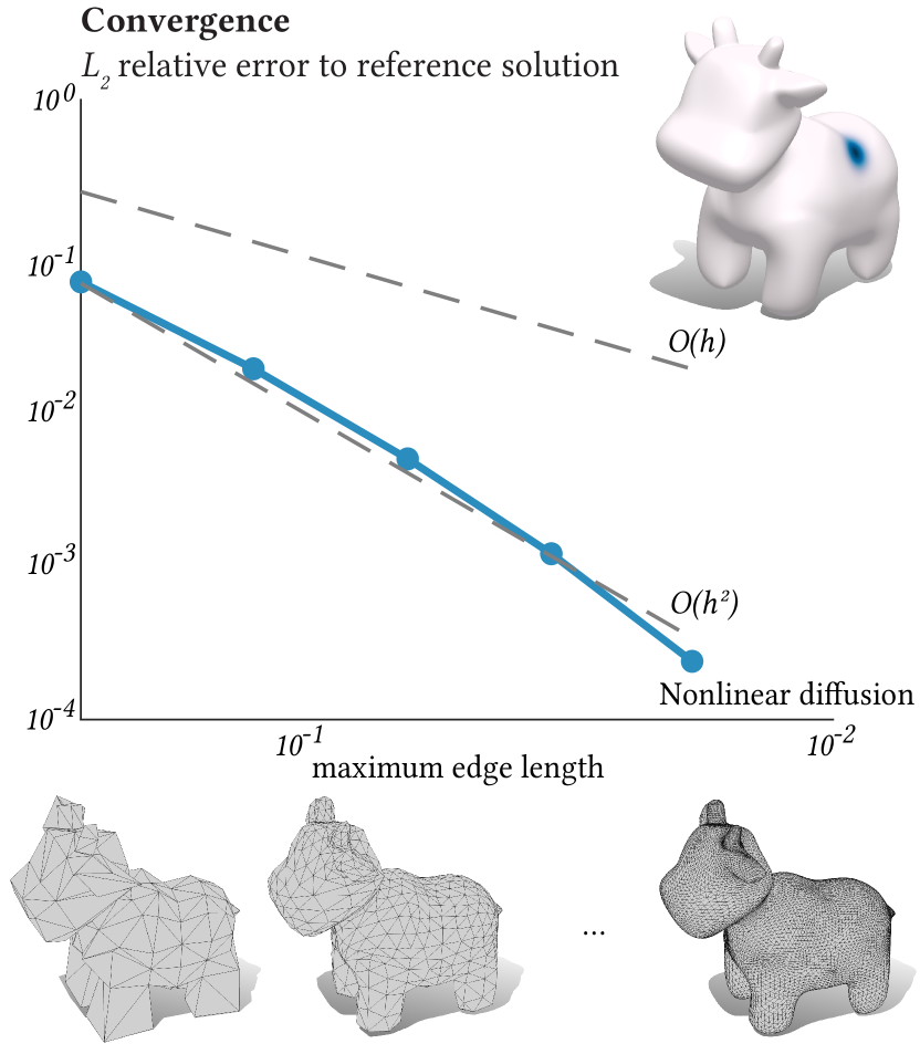
Figure 8. Convergence plot obtained for a single fixed time step $h=10^{-5}$ as the triangle mesh is refined, i.e., maximum edge length decreases ($x$-axis). The error ($y$-axis) is measured in the $L_{2}$ norm against the solution on the mesh of highest resolution.

G-equation

In this case, we simply have constraints using norms, which is already in SOCP form. Hence, we can use the conic solver efficiently without further reformulation. We implement our optimization as follows

(21) $$\begin{array}[]{r@{\ }l}\operatorname*{arg\min}_{u^{(2)}}&\textstyle\sum_{i}{\big{(}u_{n}^{(2)}\big{)}}_{i}\\ \text{subject to }&h\;\omega_{i}\textstyle\sum_{j\sim i}\big{(}\textstyle-\sum_{k=1}^{3}(\Phi_{k}\odot G_{k}u_{n}^{(2)})_{j}+\|(Gu_{n}^{(2)})_{j}\|_{2}\;\big{)}\\ &\qquad\qquad\qquad-u_{n}^{(2)}+u_{n}^{(1)}\leq 0,\;i=1,\ldots,|V|.\end{array}$$

Fokker-Planck equation

This equation is linear and requires no reformulation. Its implementation becomes:

(22) $$\begin{array}[]{r@{\ }l}\operatorname*{arg\min}_{u^{(2)}}&\textstyle\sum_{i}{\big{(}u_{n}^{(2)}}\big{)}_{i}\\ \text{subject to }&h\;\big{(}(u_{n}^{(2)}\odot(G^{\mathrm{T}}M_{F}\Phi))_{i}+\omega_{i}\textstyle\sum_{j\sim i}\textstyle\sum_{k=1}^{3}(\Phi_{k}\odot G_{k}u_{n}^{(2)})_{j}\big{)}\\ &\qquad\qquad\qquad-u_{n}^{(2)}+u_{n}^{(1)}\leq 0,\;i=1,\ldots,|V|.\end{array}$$

6. Numerical Experiments

We demonstrate the versatility of our method for a variety of PDE on surfaces and validate its performance in this section. Our experiments were carried out in Matlab $2023\mathrm{a}$, on a macOS machine with $32$GB memory. All tests were run with solver tolerance $\varepsilon^{\nicefrac{{1}}{{2}}}$, where $\varepsilon=2.22^{-16}$ is the machine precision. Code with examples is included with this paper.

6.1. PDEs on Surfaces

Our main numerical contribution is a solver capable of handling a range of linear and nonlinear parabolic PDE. As will be shown later, this solver can be coupled with existing methods found in practical applications in computer graphics (see §7). For now, we focus on demonstrating the direct use of the solver to evolve PDE with various choices of parameters and meshes. Specifically, given a velocity vector field $\Phi\in\mathbb{R}^{|F|\times 3}$ defined per face on an underlying computational mesh, we can use our framework to obtain the numerical time evolution of the $G$-equation equation and the Fokker-Planck equation as seen on the tori in Figure 7. We also refer the reader to Figures 9, 10, and 11 for illustrations of time evolution of each of our example PDE. The order of convergence for these experiments is discussed in the following subsection:

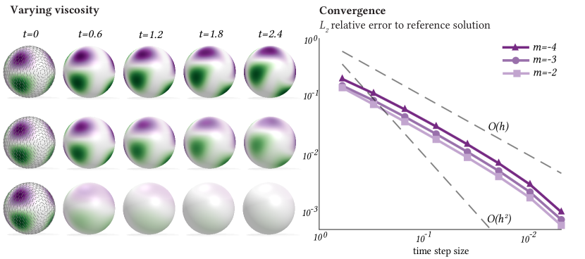
Figure 9. The effect of varying the viscosity parameter in the Fokker-Planck equation on a sphere with $81{,}920$ triangle faces and $40{,}962$ vertices. The equation is shown evolving in time on the discrete sphere with viscosity $\varepsilon=10^{-4}$ (top row), $\varepsilon=10^{-3}$ (middle row), and $\varepsilon=10^{-2}$ (bottom row).

Figure 10. Convergence plot obtained for the time evolution of the $G$-equation (top row) as the time step size is decreased ($x$-axis). The error ($y$-axis) is computed using the $L_{2}$ norm against the solution obtained with smallest step size.

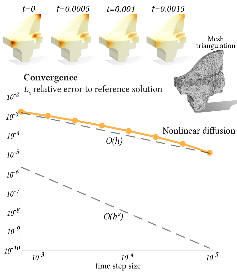
Figure 11. Convergence plot obtained for the time evolution of the nonlinear diffusion equation on a mesh with both varying triangulation quality and sharp features (top row) as the time step size is decreased ($x$-axis). The time evolution illustrations (top row) are show in exponential domain.

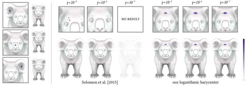
Figure 12. Small entropy coefficients can lead to numerical challenges using the state-of-the-art method (middle) for computing Wasserstein barycenters, which our logarithmic diffusion method (right) overcomes. Here, the Wasserstein barycenter of three input distributions (left) on a mesh with $99{,}994$ triangle faces and $49{,}999$ vertices is shown for different entropy coefficients.

Description

6.2. Convergence

To the best of our knowledge, there are no available closed-form solutions to the second-order parabolic PDE problems we consider on curved surfaces. To get close to measuring convergence to an analytical solution, we perform a self-convergence experiment. We use the solution for highest mesh resolution as the (nearly-)exact solution, denoted by $u^{\ast}$, and compare it to a sequence of solutions $u_{N}$ found for lower resolution meshes. We estimate the convergence order of the method by

(23) $$R=\log_{2}{\left(\frac{u^{\ast}-u_{N}}{u^{\ast}-u_{\nicefrac{{N}}{{2}}}}\right)},$$

where $N$ is either a space or time discretization size, i.e., maximum edge length size $\ell$ (for spatial convergence) or time step size $h$ (for time convergence).

In Figure 8, we present an experiment indicating convergence under spatial refinement. While our choice of discretization is standard first-order FEM, we find that the order of convergence of our method under spatial refinement is second-order (see Table 2). In Figure 10, we show an experiment to determine convergence under time refinement for the evolutionary $G$-equation, and in Figure 9, we do the same for the Fokker-Planck equation using various amounts of viscosity. The results are summarized in Table 1. For both equations convergence is of at least first-order, and first-order convergence is consistent for various amounts of viscosity as demonstrated in the evolution of the Fokker-Planck. While Strang-Marchuk splitting encourages second-order convergence, we find empirically that the first-order nature of each step’s method only guarantees first-order convergence for the scheme.

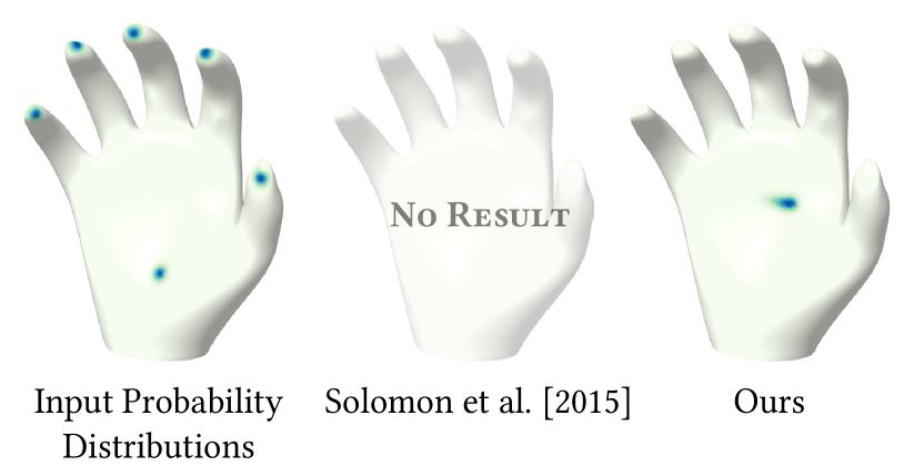
Figure 13. Barycenters with entropy value $\gamma=10^{-3}$ obtained using the convolutional method (middle) and our logarithmic diffusion method (right). The very sharp input probability distributions $\{\mu_{i}\}_{i=1}^{6}$ are shown together on the left.

6.3. Robustness

The performance of our method in meshes with varying triangulation and with sharp features is illustrated in Figure 11. In this case, our method requires smaller step sizes to achieve first-order convergence.

7. Applications

7.1. Wasserstein Barycenter

The “log-sum-exp” trick is a standard method used to stabilize numerical algorithms, including the Sinkhorn algorithm when using small amounts of entropy. This computation, however, is not possible using the method adapted to triangle meshes proposed in (Solomon et al., 2015), which corresponds to taking the logarithm of a function undergoing tiny amounts of heat diffusion. We advocate for using our numerical framework and Proposition 3.1 to solve (3) to compute the result of heat diffusion on triangle meshes directly in the logarithmic domain, rather than diffusing in the linear domain and then taking the logarithm.

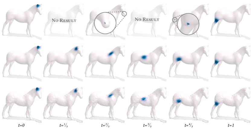
Figure 14. Wasserstein distance interpolation on a mesh with $76{,}736$ triangle faces and $38{,}370$ vertices. Top row: using the convolutional method proposed by Solomon et al. (2015). Middle row: using our logarithmic diffusion method. Bottow row: using our logarithmic diffusion method on a mesh with added uniformly random noise along normal directions. As seen on the top row, the convolutional method fails to obtain results for a small amount of entropy $\gamma=10^{-5}$.

Description

In Figure 13, we demonstrate how our log-domain diffusion algorithm outperforms the state-of-the-art in computing Wasserstein barycenters on mesh surfaces. The method in (Solomon et al., 2015) fails to output a result for the entropy coefficient $\gamma=10^{-3}$ with very sharp probability distributions as input. Even excluding this failure case, the Wasserstein barycenters obtained via the convolutional method look qualitatively wrong for a number of entropy coefficients in Figure 12, while our method remains numerically stable and obtains the expected visual results given the distributions.

7.2. Measure Interpolation

Given a pair of initial and target distributions $\mu_{0}$ and $\mu_{1}$ on a triangular mesh, the same algorithm used to compute Wasserstein barycenters can be applied with weights $(1-t,t)$ to compute a time-varying sequence of distributions $\mu_{t}$ transitioning from initial to target, moving along geodesic paths. In Figure 14, we show a comparison to the convolutional method in (Solomon et al., 2015) for the distance interpolation task. We observe again that the convolutional method fails to obtain results with a small entropy coefficient for various pairs of weights, while our method succeeds in both smooth and noisy meshes, demonstrating the robustness of our method in this task.

Figure 15. Surface moving with speed $\|\nabla u\|_{2}$. Here, the numerical comparison is done on a regular $50\times 50$ regular grid using centered differences and periodic conditions; the time step size is $h=0.01$.

7.3. Numerical Integration for Fire and Flames

Osher and Sethian (1988) provide a first-order scheme to approximate solutions to Hamilton-Jacobi equations, which is coupled with the Navier-Stokes equation by Nguyen et al. (2002) in the physical simulation of fire for graphics applications. The first method is based on an upwind generalized first-order version of Godunov’s scheme (Godunov and Bohachevsky, 1959). We compare our method for solving the $G$-equation to the method in (Osher and Sethian, 1988) and a Lax-Friedrichs scheme described in (Crandall and Lions, 1984), both standard methods of approximation for Hamilton-Jacobi equations, demonstrating how it could be effectively coupled in the same fashion for applications in the simulation of fire and flames.

The main drawback of the numerical method presented in (Osher and Sethian, 1988) is: (1) a CFL condition given the method’s explicit nature, and (2) its limitation to grids. Although our method has longer runtime per time step, it offers more stability for larger range of time step sizes (see Fig. 16), and further, it can be implemented on curved triangle mesh surfaces.

In Figure 15, we show a comparison between our framework and the method in (Osher and Sethian, 1988) for the evolution of a front $\phi$ with propagation prescribed by $\phi_{t}=\|\nabla\phi\|_{2}$, that is, essentially the $G$-equation. Since this is the limiting case where $\varepsilon=0$, we add a small amount of viscosity $\mathcal{O}(10^{-6})$ to guarantee its solutions are continuous. This is a simple regularization technique for problems without continuous solutions first introduced by Sethian (1985). We apply our framework to the regularized equation $\phi_{t}=\|\nabla\phi\|_{2}-\varepsilon\Delta\phi$ and show numerically that the dissipation created by adding viscosity performs the same as the reference method in (Osher and Sethian, 1988). We observe convergence to the same steady state and very small error at each time step of the front propagation. This comparison suggests that our method could be used as more stable component in larger simulation pipelines.

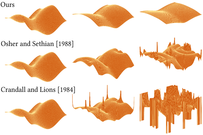
Figure 16. Standard methods used in larger graphics pipelines for simulation of fire and flames become numerically unstable for time step and spatial democratization size outside a certain CFL condition, while our method remains stable. Here, the same comparison in Fig. 15 is done, now on a regular $100\times 100$ grid and time step size $h=0.1$.

8. Discussion and Conclusion

PDE appear everywhere in geometry processing, and second-order parabolic PDE are no exception. While there are many tools to handle simpler PDE, such as the heat equation, more general parabolic PDE are a challenge to standard time integration methods and discretization schemes. Our work establishes an effective time integration and spatio-discretization strategy to solve this class of PDE under mild assumptions on triangle mesh surfaces. In addition to substantial theoretical work, we showed several numerical experiments indicating the validity of our method. We have also demonstrated how our method can be used as a numerical solver component in graphics applications. In particular, we showed how our method overcomes limitations in optimal transport tasks over geometric domains and in numerical integration schemes used for larger simulation pipelines.

While we have explored several practical implications of our framework, a number of interesting avenues for future work remain. In particular, for the Fokker-Planck equation, further experimental work includes extending results to other versions of this equation (e.g., nonlinear) and using the solutions obtained via our method together with the relationship to (7) to simulate Brownian motion on triangular surface meshes. Our work provides a meaningful first-step in this direction. On the practical side, an immediate avenue for future work is to derive an optimization algorithm to solve the problem in (11) along the lines of Edelstein et al. (2023) and compare it to our current off-the-shelf solution using CVX. On the theoretical front, we would like to explore an extension of our results to higher-order parabolic equations with Laplacian terms, such as the Kuramoto–Sivashinsky equation. Within the realm of second-order parabolic PDE of the form (1), we are hopeful that our framework would provide a means to solve systems of coupled equations.

- (1)
- Aumentado-Armstrong and Siddiqi (2017) T. Aumentado-Armstrong and K. Siddiqi. 2017. Stochastic Heat Kernel Estimation on Sampled Manifolds. Comput. Graph. Forum 36, 5 (2017), 131–138.
- Barles and Perthame (1990) G. Barles and B. Perthame. 1990. Comparison Principle for Dirichlet-Type Hamilton-Jacobi Equations and Singular Perturbations of Degenerated Elliptic Equations. Appl. Math. Optim. 21, 1 (1990), 21–44.
- Belyaev and Fayolle (2020) Alexander Belyaev and Pierre-Alain Fayolle. 2020. An ADMM-Based Scheme for Distance Function Approximation. Numer. Algorithms 84, 3 (2020), 983–996.
- Belyaev and Fayolle (2015) Alexander G. Belyaev and Pierre-Alain Fayolle. 2015. On Variational and PDE-Based Distance Function Approximations. Computer Graphics Forum 34, 8 (2015), 104–118.
- Benamou et al. (2015) Jean-David Benamou, Guillaume Carlier, Marco Cuturi, Luca Nenna, and Gabriel Peyré. 2015. Iterative Bregman Projections for Regularized Transportation Problems. SIAM Journal on Scientific Computing 37, 2 (2015), A1111–A1138.
- Bobenko and Schröder (2005) Alexander I. Bobenko and Peter Schröder. 2005. Discrete Willmore Flow. Eurographics Symposium on Geometry Processing 2005 (2005).
- Botsch et al. (2010) Mario Botsch, Leif Kobbelt, Mark Pauly, Pierre Alliez, and Bruno Levy. 2010. Polygon Mesh Processing. AK Peters / CRC Press.
- Chen et al. (2013) Zhili Chen, Renguo Feng, and Huamin Wang. 2013. Modeling Friction and Air Effects between Cloth and Deformable Bodies. ACM Trans. Graph. 32, 4, Article 88 (2013), 8 pages.
- Crandall et al. (1992) Michael G. Crandall, Hitoshi Ishii, and Pierre-Louis Lions. 1992. User’s guide to viscosity solutions of second order partial differential equations. , 67 pages. Issue 27.
- Crandall and Lions (1983) Michael G. Crandall and Pierre-Louis Lions. 1983. Viscosity Solutions of Hamilton-Jacobi Equations. Trans. Amer. Math. Soc. 277, 1 (1983), 1–42.
- Crandall and Lions (1984) M. G. Crandall and P. L. Lions. 1984. Two Approximations of Solutions of Hamilton-Jacobi Equations. Math. Comp. 43, 167 (1984), 1–19.
- Crane et al. (2013) Keenan Crane, Clarisse Weischedel, and Max Wardetzky. 2013. Geodesics in heat: A new approach to computing distance based on heat flow. ACM Trans. Graph. 32, 5 (2013), 1–11.
- Cuturi (2013) Marco Cuturi. 2013. Sinkhorn distances: Lightspeed computation of optimal transport. Advances in neural information processing systems 26 (2013).
- Desbrun et al. (1999) Mathieu Desbrun, Mark Meyer, Peter Schröder, and Alan H. Barr. 1999. Implicit Fairing of Irregular Meshes Using Diffusion and Curvature Flow. Proceedings of the 26th Annual Conference on Computer Graphics and Interactive Techniques, 317–324.
- Du and Qin (2004) Haixia Du and Hong Qin. 2004. Medial Axis Extraction and Shape Manipulation of Solid Objects Using Parabolic PDEs. In Proceedings of the Ninth ACM Symposium on Solid Modeling and Applications. Eurographics Association, Goslar, DEU, 25–35.
- Duan et al. (2004) Ye Duan, Liu Yang, Hong Qin, and Dimitris Samaras. 2004. Shape Reconstruction from 3D and 2D Data Using PDE-Based Deformable Surfaces. In Computer Vision - ECCV 2004. Springer, Berlin, Heidelberg, 238–251.
- Edelstein et al. (2023) Michal Edelstein, Nestor Guillen, Justin Solomon, and Mirela Ben-Chen. 2023. A Convex Optimization Framework for Regularized Geodesic Distances. In ACM SIGGRAPH 2023 Conference Proceedings. Association for Computing Machinery, New York, NY, USA, Article 2, 11 pages.
- Evans (2010) Lawrence C Evans. 2010. Partial Differential Equations (second ed.). Graduate Studies in Mathematics, Vol. 19. American Mathematical Society, Providence, RI.
- Fleming and Souganidis (1989) W. H. Fleming and P. E. Souganidis. 1989. On The Existence of Value Functions of Two-Player, Zero-Sum Stochastic Differential Games. Indiana Univ. Math. J. 38, 2 (1989), 293–314.
- Godunov and Bohachevsky (1959) Sergei K. Godunov and I. Bohachevsky. 1959. Finite difference method for numerical computation of discontinuous solutions of the equations of fluid dynamics. Matematičeskij sbornik 47(89), 3 (1959), 271–306.
- Grant and Boyd (2008) Michael Grant and Stephen Boyd. 2008. Graph implementations for nonsmooth convex programs. In Recent Advances in Learning and Control, V. Blondel, S. Boyd, and H. Kimura (Eds.). Springer-Verlag Limited, Berlin, Heidelberg, 95–110. http://stanford.edu/~boyd/graph_dcp.html.
- Grant and Boyd (2014) Michael Grant and Stephen Boyd. 2014. CVX: Matlab Software for Disciplined Convex Programming, version 2.1. http://cvxr.com/cvx.
- Gu et al. (2021) Haotian Gu, Jack Xin, and Zhiwen Zhang. 2021. Error Estimates for a POD Method for Solving Viscous G-Equations in Incompressible Cellular Flows. SIAM Journal on Scientific Computing 43, 1 (2021), A636–A662.
- Hitoshi Ishii and Yan (2022) Lin Wang Hitoshi Ishii, Kaizhi Wang and Jun Yan. 2022. Hamilton–Jacobi equations with their Hamiltonians depending Lipschitz continuously on the unknown. , 417-452 pages.
- Hong et al. (2007) Jeong-Mo Hong, Tamar Shinar, and Ronald Fedkiw. 2007. Wrinkled Flames and Cellular Patterns. ACM Trans. Graph. 26, 3 (2007), 47–52.
- Huguet et al. (2023) Guillaume Huguet, Alexander Tong, María Ramos Zapatero, Christopher J. Tape, Guy Wolf, and Smita Krishnaswamy. 2023. Geodesic Sinkhorn for Fast and Accurate Optimal Transport on Manifolds. (2023).
- Ishii (1987) Hitoshi Ishii. 1987. Perron’s method for Hamilton-Jacobi equations. Duke Mathematical Journal 55, 2 (1987), 369–384.
- Jost (2011) Jürgen Jost. 2011. The Laplace Operator and Harmonic Differential Forms. Springer, Berlin, Heidelberg, Chapter 3, 89–131.
- Kato (1974) Tosio Kato. 1974. On the Trotter-Lie product formula. Proceedings of the Japan Academy 50, 9 (1974), 694–698.
- Leatham et al. (2022) T. A. Leatham, D. M. Paganin, and K. S. Morgan. 2022. X-ray dark-field and phase retrieval without optics, via the Fokker-Planck equation. IEEE Transactions on Medical Imaging 42, 6 (2022), 1681–1695.
- Liu et al. (2013) Yu-Yu Liu, Jack Xin, and Yifeng Yu. 2013. A numerical study of turbulent flame speeds of curvature and strain G-equations in cellular flows. Physica D: Nonlinear Phenomena 243, 1 (2013), 20–31.
- Léonard (2014) Christian Léonard. 2014. A survey of the Schrödinger problem and some of its connections with optimal transport. Discrete and Continuous Dynamical Systems 34, 4 (2014), 1533–1574.
- Marchuk (1988) Gury Ivanovich Marchuk. 1988. Splitting Methods. (1988), 264.
- Medved et al. (2020) Andrei Medved, Riley Davis, and Paula A. Vasquez. 2020. Understanding Fluid Dynamics from Langevin and Fokker–Planck Equations. Fluids 1, Article 40 (2020).
- Nguyen et al. (2002) Duc Quang Nguyen, Ronald Fedkiw, and Henrik Wann Jensen. 2002. Physically Based Modeling and Animation of Fire. ACM Trans. Graph. 21, 3 (2002), 721–728.
- Nielsen et al. (2022) Michael B. Nielsen, Morten Bojsen-Hansen, Konstantinos Stamatelos, and Robert Bridson. 2022. Physics-Based Combustion Simulation. ACM Trans. Graph. 41, 5, Article 176 (2022), 21 pages.
- O’Brien et al. (2002) James F. O’Brien, Adam W. Bargteil, and Jessica K. Hodgins. 2002. Graphical Modeling and Animation of Ductile Fracture. ACM Trans. Graph. 21, 3 (2002), 291–294.
- Osher and Sethian (1988) Stanley Osher and James A Sethian. 1988. Fronts propagating with curvature-dependent speed: Algorithms based on Hamilton-Jacobi formulations. J. Comput. Phys. 79, 1 (1988), 12–49.
- Sethian (1985) James A Sethian. 1985. Curvature and the evolution of fronts. Communications in Mathematical Physics 101, 4 (1985), 487–499.
- Smolka and Wojciechowski (1997) Bogdan Smolka and Konrad W. Wojciechowski. 1997. Contrast enhancement of badly illuminated images based on Gibbs distribution and random walk model. In Computer Analysis of Images and Patterns. Springer, Berlin, Heidelberg, 271–278.
- Solomon et al. (2015) Justin Solomon, Fernando de Goes, Gabriel Peyré, Marco Cuturi, Adrian Butscher, Andy Nguyen, Tao Du, and Leonidas Guibas. 2015. Convolutional Wasserstein Distances: Efficient Optimal Transportation on Geometric Domains. ACM Trans. Graph. 34, 4, Article 66 (jul 2015), 11 pages.
- Sommeijer et al. (1998) B.P. Sommeijer, L.F. Shampine, and J.G. Verwer. 1998. RKC: An explicit solver for parabolic PDEs. J. Comput. Appl. Math. 88, 2 (1998), 315–326.
- Strang (1968) Gilbert Strang. 1968. On the construction and comparison of different splitting schemes. SIAM J. Numer. Anal. 5, 3 (1968), 506–517.
- Toh et al. (1999) K. C. Toh, M. J. Todd, and R. H. Tütüncü. 1999. SDPT3 — A Matlab software package for semidefinite programming, Version 1.3. Optimization Methods and Software 11, 1-4 (1999), 545–581.
- Trotter (1959) H. F. Trotter. 1959. On the Product of Semi-Groups of Operators. Proc. Amer. Math. Soc. 10, 4 (1959), 545–551.
- Tütüncü et al. (2003) Reha H. Tütüncü, Kim-Chuan Toh, and Michael J. Todd. 2003. Solving semidefinite-quadratic-linear programs using SDPT3. Mathematical Programming 95 (2003), 189–217. Issue 2.
- Villani (2003) Cédric Villani. 2003. Topics in Optimal Transportation. Graduate Studies in Mathematics, Vol. 58. American Mathematical Society, Providence, RI.
- Williams (1985) F. A. Williams. 1985. Turbulent Combustion. In The Mathematics of Combustion, John D. Buckmaster (Ed.). Society for Industrial and Applied Mathematics, Philadelphia, PA, 97–131.
- Witkin and Kass (1991) Andrew Witkin and Michael Kass. 1991. Reaction-Diffusion Textures. In Proceedings of the 18th Annual Conference on Computer Graphics and Interactive Techniques. Association for Computing Machinery, New York, NY, USA, 299–308.
- Xu et al. (2006) Guoliang Xu, Qing Pan, and Chandrajit L. Bajaj. 2006. Discrete surface modelling using partial differential equations. Computer Aided Geometric Design 23, 2 (2006), 125–145.
- Yan and Osher (2011) Jue Yan and Stanley Osher. 2011. A local discontinuous Galerkin method for directly solving Hamilton–Jacobi equations. J. Comput. Phys. 230, 1 (2011), 232–244.