SN 2015da: Late-time observations of a persistent superluminous Type IIn supernova with post-shock dust formation

Abstract

We present photometry and spectroscopy of the slowly evolving superluminous Type IIn supernova (SN) 2015da. SN 2015da is extraordinary for its very high peak luminosity, and also for sustaining a high luminosity for several years. Even at 8 yr after explosion, SN 2015da remains as luminous as the peak of a normal SN II-P. The total radiated energy integrated over this time period (with no bolometric correction) is at least $1.6\times 10^{51}$ erg (or 1.6 FOE). Including a mild bolometric correction, adding kinetic energy of the expanding cold dense shell of swept-up circumstellar material (CSM), and accounting for asymmetry, the total explosion kinetic energy was likely 5–10 FOE. Powering the light curve with CSM interaction requires an energetic explosion and 20 M_⊙ of H-rich CSM, which in turn implies a massive progenitor system $>$30 M_⊙. Narrow P Cyg features show steady CSM expansion at 90 km s^-1, requiring a high average mass-loss rate of $\sim$0.1 M_⊙ yr^-1 sustained for 2 centuries before explosion (although ramping up toward explosion time). No current theoretical model for single-star pre-SN mass loss can account for this. The slow CSM, combined with broad wings of H$\alpha$ indicating H-rich material in the unshocked ejecta, disfavour a pulsational pair instability model for the pre-SN mass loss. Instead, violent pre-SN binary interaction is a likely cuprit. Finally, SN 2015da exhibits the characteristic asymmetric blueshift in its emission lines from shortly after peak until the present epoch, adding another well-studied superluminous SNe IIn with unambiguous evidence of post-shock dust formation.

1 INTRODUCTION

Since the first well-observed example of SN 2006gy, superluminous supernovae (SLSNe) have presented a significant challenge for stellar evolution theory. Hydrogen-deficient examples (Quimby et al., 2011), usually referred to as SLSNe Ic, show broad lines in their spectra and have been modeled as the result of post-explosion energy deposition by a magnetar wind (Woosley, 2010; Kasen & Bildsten, 2010). On the other hand, SLSNe with hydrogen lines usually exhibit relatively narrow components in their line profiles, and are thus classified as SLSNe IIn. These, like their more modest-luminosity analogs (i.e., regular SNe IIn; Schlegel 1990; Filippenko 1997), are thought to be powered by shock interaction with dense circumstellar material (CSM). Key challenges for stellar evolution posed by SLSNe IIn are getting massive progenitors to evolve up to the time of core collapse with their H envelope intact, then shedding much of that H envelope in sudden bursts of mass loss just prior to core collapse, and finally getting massive progenitors to explode successfully with higher than average energy (see Smith et al., 2007, 2010; Groh et al., 2013).

CSM interaction can produce wide diversity in the observed properties of SNe IIn, since any type of SN explosion can, in principle, have dense CSM, and that CSM can vary in its mass, radial distribution, and geometry (see Smith, 2017, for a review of interacting SNe). Some have only a small additional luminosity, whereas others become extraordinarily luminous (as in the case of SLSNe IIn). Some have CSM interaction signatures that are fleeting, fading in only a few days (like the recent example of SN 2023ixf in M101; Jacobson-Galan et al. 2023; Smith et al. 2023; Bostroem et al. 2023), and others have extremely strong interaction that can persist for decades (as in the prolonged cases of SN 1988Z and SN 2005ip; Smith et al. 2017, 2009b; Fox et al. 2010; Williams et al. 2002). Large fluctuations in pre-SN mass loss may lead to highly variable CSM interaction, observed as bumps or dips in the late-time light curves (Nyholm et al., 2017; Smith et al., 2017). CSM interaction can also lead to efficient dust formation in the rapidly cooling post-shock layers, indicated by a combination of excess infrared (IR) emission and blueshifted emission-line profiles (Smith et al., 2008a, 2009b, 2012; Gall et al., 2014; Smith & Andrews, 2020). Ongoing CSM interaction can cause SNe IIn to appear as luminous IR sources for many years, as pre-shock CSM dust is continually heated by the advancing shock (Fox et al., 2013; Fox & Filippenko, 2013; Fox et al., 2015, 2020). Spectral signatures of dust formation are discussed later in this paper.

SNe IIn require astounding progenitor mass loss to produce their dense CSM. The least of these require mass loss at around $10^{-3}$ M_⊙ yr^-1, which would overlap with the strongest known examples of steady stellar winds, like the current wind of $\eta$ Carinae (Smith et al., 2003b; Hillier et al., 2006) or those of the most extreme known red supergiants (RSGs) like VY CMa (Smith et al., 2009a, b; Decin et al., 2006). Normal RSG winds are 100–1000 times weaker (Beasor et al., 2020). The majority of SNe IIn require even higher mass-loss rates of $10^{-2}$ to $10^{-1}$ M_⊙ yr^-1 or more, far beyond the limiting capability of any known radiatively driven steady stellar wind (Smith & Owocki, 2006; Smith, 2014). This points instead to episodic, eruptive, and explosive mass-loss mechanisms. The only well-established observed precedent for this mode of mass loss is the giant eruptions of luminous blue variables (LBVs; Smith et al. 2011b). The mechanism for these eruptions remains debated, but may arise from super-Eddington continuum-driven winds (Smith & Owocki, 2006; Owocki et al., 2004, 2017; Quataert et al., 2016) or violent binary interaction (Smith et al., 2018; Soker & Tylenda, 2006). There are many cases of SNe IIn and SLSNe IIn in between the observed extremes, representing a continuum in CSM properties (e.g., Dickinson et al. 2023).

In SLSNe IIn, the luminosity peaks at early times are likely powered by diffusion of shock-deposited energy in an opaque CSM envelope, analogous to a delayed shock breakout with photons degraded to optical wavelengths. This was first proposed to explain the main peak of SN 2006gy (Smith & McCray, 2007), and was subsequently adopted more generally for SNe IIn (Balberg & Loeb, 2011; Chevalier & Irwin, 2011). This mechanism leads to extremely high efficiency for converting kinetic energy into radiation (Smith & McCray, 2007; van Marle et al., 2010). At later times when the optical depth drops, we can see the shock interaction more directly, and SNe IIn can be luminous in X-rays that escape the shock-interaction zone (Chandra et al., 2009, 2012, 2022; Pooley et al., 2002; Tsuna et al., 2021).

In order to account for the high luminosity of SLSNe through CSM interaction, the required total amount of CSM mass in SLSNe is extreme, typically requiring 5–10 M_⊙ (sometimes even 20–25 M_⊙ or more) of CSM ejected by the progenitor shortly before exploding (Dickinson et al., 2023; Nicholl et al., 2020; Rest et al., 2011; Smith & McCray, 2007; Smith et al., 2008b, 2010; Woosley et al., 2007). When one factors in the mass of the compact remnant, the SN ejecta, and mass lost by winds during the star’s lifetime, this mass budget points to quite massive progenitor stars for some SLSNe IIn, in some cases with intial masses that must exceed 40–50 M_⊙. High-mass progenitors retaining their H envelopes until shortly before death, when they are ejected in LBV-like eruptions, directly contradicts predictions of traditional stellar-evolution models. Such stars are expected to lose their H envelopes in winds during their lifetime, perhaps passing through a transitory LBV phase, before becoming H-free Wolf-Rayet (WR) stars that die as SNe Ibc (Chiosi & Maeder, 1986; Woosley et al., 1993; Maeder & Meynet, 2000; Heger et al., 2003). Some of this disagreement may be alleviated by reduced wind mass-loss rates (see the review by Smith, 2014, for an extended discussion). These more realistic lower mass-loss rates have, however, not yet percolated into the most commonly used stellar evolution model grids. Even if more realistic lower mass-loss rates allow massive stars with $M_{\rm ZAMS}\ga 30\,{\rm M}_{\odot}$ to retain their H envelopes until death, their successful energetic explosion and their bursts of pre-SN mass loss still pose a theoretical challenge.

The question of how long the strong CSM interaction lasts is particularly important for diagnosing the underlying physical mechanism(s) that may have produced dense CSM. An observed estimate for the expansion speed of the CSM can help constrain the time period before core collapse when the CSM was ejected. Some proposed mechanisms for episodic pre-SN mass loss include energy transferred to the envelope by wave driving in advanced nuclear burning phases (Quataert & Shiode, 2012; Shiode & Quataert, 2014; Fuller, 2017; Fuller & Ro, 2018; Wu & Fuller, 2021), the pulsational pair instability or other late-phase burning instabilities (Woosley et al., 2007; Woosley, 2017; Arnett & Meakin, 2011; Smith & Arnett, 2014; Renzo et al., 2020), or an inflation of the progenitor’s radius (perhaps caused by the previous mechanisms) that triggers violent binary interaction like collisions or mergers before core collapse (Smith & Arnett, 2014) or mergers with compact companions (Fryer & Woosley, 1998; Schrøder et al., 2020). Of these various mechanisms, only the ones with binary interaction predict highly asymmetric distributions of CSM (disk-like or bipolar), relevant to asymmetric line-profile shapes and high polarization seen in SNe IIn (Bilinski et al., 2023). In terms of timescale, wave driving only operates for about 1 yr during Ne and O burning, and is therefore too short to account for SNe IIn and SLSNe IIn, which require heavy mass loss for decades or centuries. The pulsational pair instability also operates primarily during O burning, although its timescale can be extended significantly in some cases owing to Kelvin-Helmholtz relaxation after a powerful pulse (Woosley, 2017; Renzo et al., 2020). However, the pair instability should only operate in extremely massive stars and is therefore too rare to account for SNe IIn that make up $\sim$8 % of ccSNe (Smith et al., 2011a). It is a good candidate to explain the pre-SN mass loss for some of the rare SLSNe IIn (Woosley et al., 2007), although as we argue below, not for SN 2015da.

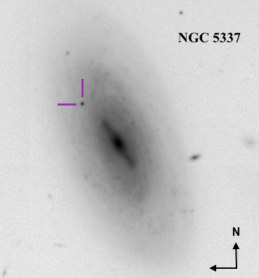
Figure 1: A late-time LBT/MODS $r$-band image of SN 2015da and its barred spiral host galaxy NGC 5337 taken on 2018 January 16 (day 1104). The SN position is indicated by the violet crosshairs.

Table 1: SLOTIS $BVRI$ photometry

MJD	$B$	$\sigma$	$V$	$\sigma$	$R$	$\sigma$	$I$	$\sigma$
	(mag)	(mag)	(mag)	(mag)	(mag)	(mag)	(mag)	(mag)
57148.7	17.87	0.23	16.56	0.06	15.66	0.03	15.02	0.04
57150.7	17.60	0.21	16.57	0.07	15.69	0.05	15.05	0.04
57152.8	17.66	0.15	16.56	0.08	15.72	0.04	15.03	0.03
57162.7	17.34	0.30	16.71	0.10	15.79	0.05	15.12	0.06
57168.7	17.80	0.14	16.84	0.09	15.89	0.02	15.16	0.04
57171.7	17.88	0.27	16.73	0.12	15.87	0.03	15.15	0.05
57174.7	17.24	0.37	16.80	0.14	15.91	0.03	15.21	0.05
57177.7	17.67	0.21	16.96	0.11	15.94	0.03	15.18	0.05
57192.7	…	…	16.92	0.14	15.97	0.04	…	…
57195.7	…	…	16.85	0.11	16.02	0.05	…	…
57387.0	…	…	…	…	16.84	0.04	16.43	0.09
57441.9	19.13	0.20	…	…	17.15	0.06	16.89	0.04
57825.9	…	…	…	…	18.39	0.08	…	…
57902.7	…	…	…	…	18.55	0.06	…	…

In this paper, we discuss the long-lasting superluminous Type IIn event SN 2005da (also known as PSN J13522411+3941286), discovered in the barred spiral NGC 5337 (see Fig. 1). The photometric and spectroscopic evolution have already been discussed in detail by Tartaglia et al. (2020, T20 hereafter), and we refer the reader to that paper for background information about its discovery, host galaxy and environment, and early-time evolution. To be consistent with T20, we adopt the same values for the distance $d=53.2$ Mpc, host-galaxy redshift $z=0.0071$, distance modulus $m-M=33.63$ mag, line-of-sight reddening $E(B-V)=0.98$ mag (combined 0.01 mag Galactic and 0.97 mag host-galaxy reddening), and metallicity $\sim 0.6$ Z_⊙. For the sake of comparison, we also adopt the T20 explosion UTC date of 2015 Jan. 8.45 (JD = 2,457,030.95), which was well constrained by observations to be about 1.5 days before the first detection. This makes SN 2015da an unusual case of being a nearby superluminous SN IIn discovered within a few days of explosion while still in its early rise, similar to SN 2006gy (Smith et al., 2007), but closer to us. Another well-studied SN IIn, SN 2010jl, was even closer at $\sim$49 Mpc (Smith et al., 2011c) and spectroscopically similar to SN 2015da (T20), but discovered later in its evolution around the time of peak brightness (Stoll et al., 2011). Compared to T20, we present an independent and complementary set of photometric and spectroscopic data that shows similar overall evolution, so our discussion of the observations and results in Section 2 and 3 are brief. However, a difference is that we include a series of higher-resolution spectra over a longer time, and we also include photometry extended to later times. In our analysis, we briefly discuss areas where our interpretation is complementary to that of T20 as we discuss the overall energy and mass budget of SN 2015da, but we also highlight areas where our analysis and interpretation differ from those of T20, particularly in the interpretation of the emission-line-profile evolution.

2 OBSERVATIONS

2.1 Imaging

After discovery of SN 2015da, we added its field to the queue of the robotic Super-LOTIS 24 inch telescope (SLOTIS; Williams et al., 2008) on Kitt Peak for multifilter ($B$, $V$, $R$, and $I$) follow-up observations. The seeing varied in the range $\sim$2$-$4 arcsec. Images were automatically reduced and calibrated using a custom pipeline, and aperture photometry was performed manually. Table 1 lists the resulting SLOTIS photometry. We also obtained a series of $B$, $V$, and $R$ images using the Mont4k CCD on the 61 inch Kuiper telescope on Mt. Bigelow (Fontaine et al., 2014); the seeing was typically 1$-$2 arcsec. Aperture photometry was performed manually. Some of the reference stars were outside the field of view or saturated, and were thus excluded from the reduction. Table 2 summarizes the results.

Table 2: Kuiper/Mont4k $BVR$ photometry

MJD	$B$	$\sigma$	$V$	$\sigma$	$R$	$\sigma$
	(mag)	(mag)	(mag)	(mag)	(mag)	(mag)
57166.8	…	…	16.79	0.07	15.88	0.06
57465.9	19.16	0.08	18.29	0.08	17.19	0.04
57495.9	19.26	0.08	18.41	0.08	17.38	0.03
57521.8	19.31	0.08	18.56	0.06	17.52	0.02
57543.7	19.54	0.07	18.62	0.10	17.64	0.04
57578.7	…	…	18.72	0.08	17.77	0.02
57864.9	…	…	…	…	18.48	0.05
57923.8	…	…	…	…	18.59	0.04
58109.0	…	…	…	…	18.73	0.05

Table 3: Late-time optical photometry

UTC Date	Age (days)	Tel./Instr.	filt.	mag	$\sigma$
2018-01-16	1104	LBT/MODS	$g$	20.17	0.07
2018-01-16	1104	LBT/MODS	$r$	19.28	0.03
2019-06-01	1605	MMT/Bino	$r$	19.47	0.05
2022-03-03	2582	LBT/MODS	$g$	21.19	0.10
2022-03-03	2582	LBT/MODS	$r$	20.21	0.10
2022-03-25	2604	MMT/Bino	$g$	21.09	0.09
2022-03-25	2604	MMT/Bino	$r$	20.15	0.07
2022-03-25	2604	MMT/Bino	$i$	20.38	0.10
2022-05-06	2646	LBT/MODS	$g$	21.17	0.12
2022-05-06	2646	LBT/MODS	$r$	20.18	0.08

Table 4: Near-infrared photometry

MJD	Age	Tel.	$J$	$\sigma_{J}$	$H$	$\sigma_{H}$	$K$	$\sigma_{K}$
	(days)		(mag)	(mag)	(mag)	(mag)	(mag)	(mag)
57144	114	UKIRT	14.07	0.01	13.63	0.01	13.27	0.02
57178	148	UKIRT	14.41	0.01	13.94	0.01	13.46	0.02
57193	163	UKIRT	14.52	0.01	14.06	0.01	13.55	0.02

Late time $g$-, $r$-, and $i$-band images were also obtained between 2018 to 2022 using the imaging mode of the Multi Object Double Spectrograph (Byard & O’Brien, 2000, MODS) mounted on the 2$\times$8.4 m Large Binocular Telescope (LBT), as well as the imaging mode of Binospec (Fabricant et al., 2019) on the 6.5 m MMT. An LBT/MODS $r$-band image is shown in Figure 1. Photometry measured from these late-time MMT and LBT images is listed in Table 3.

Figure 2 shows our optical $V/g$, $R/r$, and $I$-band photometry from SLOTIS, KUIPER, and LBT converted to absolute magnitudes using the adopted distance and reddening corrections noted in the Introduction. For comparison, we also show the $R$-band photometry of SN 2015da from T20, as well as SLSN IIn $R$ light curves of SN 2006gy (Smith et al., 2007) and SN 2010jl (Fransson et al., 2014).

Three sets of near-IR $JHK$-band images were obtained during the same period as the SLOTIS data, using the UK Infrared Telescope (UKIRT) Wide Field Camera instrument (WFCAM; Hodgkin et al., 2009). The seeing, estimated from the full width at half-maximum intensity (FWHM) of stars on the CCD frame, varied from $1^{\prime\prime}$ to $2^{\prime\prime}$. Aperture photometry was performed manually, and the magnitudes were calibrated using the same reference stars from SLOTIS. The results are summarised in Table 4.

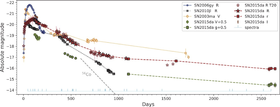
Figure 2: Absolute magnitude light curve of SN 2015da compared to other SLSNe IIn. $R$-band light curve of SN 2006gy (Smith et al., 2007) in blue circles and SN 2010jl (Fransson et al., 2014) in grey/black squares, plus the $V$-band light curve of SN 2003ma in orange (Rest et al., 2011), are given for comparison. The $R$ light curve of SN 2015da from T20 is shown with light-red unfilled stars and a dashed line. Our new SN 2015da photometry is plotted for $V$ (green solid circles), $R$ (red stars), and $I$ (brown diamonds). Photometry from Kuiper images has black outlines, while SLOTIS points do not. For the Kuiper and SLOTIS $R$ photometry, we have subtracted a constant baseline flux to correct for galaxy light in the aperture. The late-time LBT/MODS and MMT/Binospec photometry in $g$ and $r$ is shown with squares, but using the same fill colours as $V$ and $R$. The ⁵⁶Co decay rate with an arbitrary luminosity is also shown for comparison (grey dashed line), and times of our spectra are indicated with light-blue tick marks at the bottom.

Table 5: Log of spectral observations of SN 2015da

Date	Age	Tel./Instr.	Range
UTC	(days)		(Å)
2015-02-23	46	Keck/DEIMOS	4850–7500
2015-03-23	74	MMT/BCH	5700–7000
2015-04-15	97	LBT/MODS	6500–8600
2015-05-01	113	MMT/BCH	5730–7030
2015-05-11	123	MMT/BCH	5710–7010
2015-06-13	156	MMT/BCH	5710–7010
2015-07-24	197	Shane/Kast	3400–10800
2015-09-06	241	Shane/Kast	3400–10.800
2016-02-11	399	Shane/Kast	3400–10,800
2016-02-16	404	MMT/BCH	5700–7000
2016-04-17	465	Bok/B&C	4000–8300
2016-06-04	513	MMT/BCH	5700–7000
2016-06-08	517	Bok/B&C	4000–8000
2016-06-14	523	Bok/B&C	3700–8300
2016-07-14	553	Bok/B&C	3900–8100
2017-01-05	728	Bok/B&C	5500–7500
2017-01-07	730	MMT/BCH	5720–7020
2017-03-04	786	MMT/BCH	5720–7020
2017-03-22	804	MMT/BCH	5750–7050
2017-05-14	857	Bok/B&C	4500–8000
2017-05-20	863	MMT/BCH	5750–7050
2017-05-21	864	MMT/BCH	3700–9000
2017-06-30	904	MMT/BCH	5720–7020
2017-12-03	1060	MMT/BCH	5830–7130
2017-12-29	1086	MMT/RCH	6170–6970
2017-12-29	1086	MMT/RCH	8230–8980
2018-04-15	1193	MMT/BCH	5720–7020
2018-06-18	1257	MMT/BCH	5720–7020
2019-01-05	1457	Keck/LRIS	3660–10,300
2020-12-14	2167	MMT/BCH	5740–7040
2021-01-13	2197	MMT/BCH	5700–7000
2021-06-11	2345	MMT/BCH	5700–7000
2021-12-06	2523	MMT/BCH	5700–7000
2022-03-24	2603	LBT/MODS	6500–8600
2023-04-27	3030	MMT/BCH	5700–7000

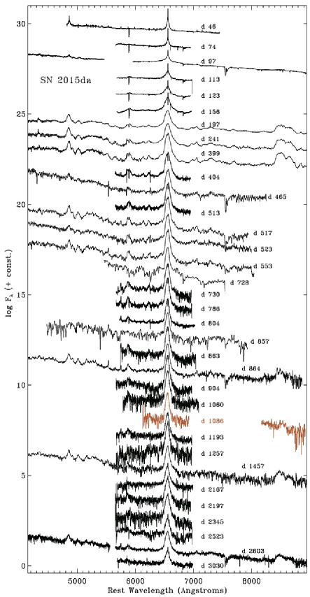
Figure 3: A series of low- and moderate-resolution spectra of SN 2015da from MMT, LBT, Keck, Lick, and Bok (see Table 5).

2.2 Spectroscopy

We obtained spectra of SN 2015da using the 6.5 m MMT with three different instruments, including the Bluechannel (BC) spectrograph, the Redchannel (RC) spectrograph, and BinoSpec (Fabricant et al., 2019). Each MMT Bluechannel observation was taken with a 1.0 arcsec slit and either the 1200 lines mm^-1 grating covering a range of $\sim$5700$-$7000 Å, or the 300 lines mm^-1 grating, covering $\sim$3600$-$9000 Å. MMT/Redchannel observations also used the 1200 lines mm^-1 grating with two different tilts centred on H$\alpha$ and the Ca ii near-IR triplet. Standard reductions were carried out using IRAF including bias subtraction, flat-fielding, and optimal extraction of the spectra. Flux calibration was achieved using spectrophotometric standards observed at an airmass similar to that of each science frame, and the resulting spectra were median combined into a single one-dimensional (1D) spectrum for each epoch. Late epochs of visual-wavelength spectra obtained with Binospec on the MMT used the 600 lines mm^-1 grating centred on 6300 Å (covering a range of $\sim$5100$-$7500 Å) and with a $1.0^{\prime\prime}$ slit. All data were reduced using the Binospec pipeline (Kansky et al., 2019), which includes an internal flux calibration into relative flux units from throughput measurements of spectrophotometric standard stars.

Additional spectra were obtained using MODS on the LBT, and at the W. M. Keck Observatory using the Deep Imaging Multi-Object Spectrograph (DEIMOS; Faber et al., 2003) and the Low-Resolution Imaging Spectrometer (LRIS; Oke et al., 1995). We also obtained a few epochs of low-resolution optical spectra with the Boller & Chivens (B&C) spectrograph mounted on the 2.3 m Bok telescope at Kitt Peak, as well as the Kast spectrograph (Miller & Stone, 1993) on the Lick 3 m Shane reflector. Data reduction for these followed standard reduction for point sources in long-slit optical spectra, as above, except that the LRIS spectrum on day 1457 was reduced using the LPipe data-reduction pipeline (Perley, 2019). All visual-wavelength spectra are corrected for $z=0.0067$ (rather than $z=0.0071$; see below) and a reddening of $E(B-V)=0.98$ mag. Our low/moderate-resolution spectra are plotted in Figure 3, and details of the spectroscopic observations are summarised in Table 5.

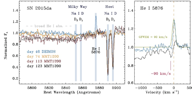
Figure 4: Left: Region of the spectrum around the interstellar Na i D lines as seen in our moderate-resolution spectra at early times around peak luminosity. Wavelengths for the Na i D doublet in both the Milky Way (blueshifted here) and in the host galaxy are indicated by the light-blue vertical bars, as is the wavelength of He i $\lambda$5876. Note that these spectra have been corrected for a redshift of $z=0.0067$, which differs by $-120$ km s^-1 from the centroid redshift of the host galaxy, presumably due to galactic rotation at SN 2015da’s location. Narrow He i $\lambda$5876 seen on day 46 transitions to weaker emission and P Cygni absorption at later epochs, and the very broad He i $\lambda$5876 absorption from the SN ejecta (in the left side of this panel) grows in strength. Right: Zoom-in on He i $\lambda$5876 showing only the day 46 and day 123 spectra. The $-$90 km s^-1 velocity of the P Cygni trough on day 123 is marked in magenta, and a Gaussian with a FWHM (GFWHM) of 90 km s^-1 is shown in green, centred on zero velocity.

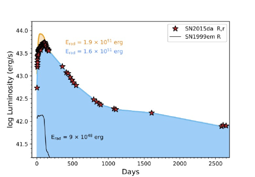
Figure 5: The $r/R$-band light curve of SN 2015da converted to L_⊙ values. The blue curve is interpolated between the photometry, and the area under the curve corresponds to a total radiated energy $E_{\rm rad}$ of $1.6\times 10^{51}$ erg with no bolometric correction applied. The orange curve, which only differs at early times, shows an approximation of the “pseudo-bolometric” light curve of SN 2015da from T20. In this case the integrated radiation would be $E_{\rm rad}=1.9\times 10^{51}$ erg. The light curve and the much lower integrated radiation measured the same way are shown for SN 1999em (black), for comparison.

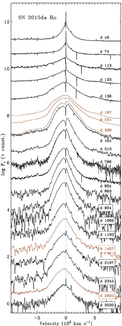
Figure 6: Spectral evolution of the H$\alpha$ line profile as seen in a selection of spectra emphasising those with higher spectral resolution. Some lower-resolution spectra are shown (plotted in orange) because they sample times when we lack higher-resolution spectra, or they have good signal-to-noise ratio (S/N) at times when higher-resolution spectra have relatively poor S/N. The narrow P Cygni profiles are missing from these spectra owing to their lower resolution. Asymmetric blueshifted profiles begin to develop after day 100 and continue until the latest observations.

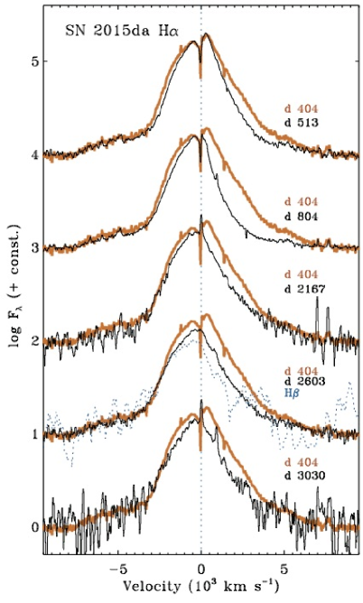
Figure 7: A few late-time H$\alpha$ profiles from Figure 6, where five late epochs (days 513, 804, 2167, 2603, and 3030) are shown in black, each plotted on top of the day 404 H$\alpha$ profile (orange). For day 2603, the H$\beta$ profile is also scaled and overplotted (dashed blue) for comparison.

3 RESULTS

3.1 Narrow Na i D, Extinction, and He i

Figure 4 shows a detail of the region of the spectrum around the interstellar Na i D lines in our higher-resolution spectra obtained at early times when SN 2015da was brightest. Strong Na i D absorption is detected from the interstellar medium of the host galaxy, but Na i D is not detected from the Milky Way (the spectra in Fig. 4 are corrected for redshift, so the Milky Way components appear blueshifted as noted in the caption). This agrees qualitatively with the low foreground reddening in the Milky Way and the relatively high reddening inferred for the host (T20). We measure equivalent widths (EWs) of 1.3 Å and 1.1 Å ($\pm$0.05 Å) for the pair of lines in the host galaxy, averaged over the four spectra in Figure 4. This is in reasonable agreement with the EWs measured for these lines already by T20, who noted that they are too strong to use the standard relationship for interstellar reddening (Poznanski et al., 2012). We do not alter the reddening estimate, and as noted above, we adopt the value used by T20 of $E(B-V)=0.98$ mag for the total line-of-sight reddening.

In examining this region of the spectrum, however, there are a few notable points. First, we needed a slightly different redshift than that of the host galaxy in order to match the observed Na i D lines to their expected laboratory wavelengths (shown by the light-blue bars in Fig. 4). As noted in the Introduction, the host galaxy NGC 5337 has a centroid velocity that gives $z=0.0071$, but the redshift used to correct the spectra in Fig. 4 is $z=0.0067$. In other words, host-galaxy interstellar gas along the line of sight to SN 2015da is blueshifted by $-$120 km s^-1 compared to the centroid velocity of the host, with the difference most likely due to galactic rotation at the location of SN 2015da. This is useful when interpreting the velocities of narrow components throughout the paper. For all remaining spectra in the paper, we correct the redshift using $z=0.0067$.

Second, this region of the spectrum reveals interesting behaviour of He i $\lambda$5876, and the adopted redshift correction impacts its interpretation. We see that He i $\lambda$5876 appears as a narrow emission line in our earliest spectrum (day 46), but after that the emission line weakens, and goes into absorption. As time proceeds, we also see increasing strength of broad P Cygni absorption, indicating that we are detecting the fast SN ejecta even at times near peak brightness.

The right panel of Fig. 4 shows a detail of He i $\lambda$5876. Here, zero velocity is defined by the alignment of the nearby Na i D lines. Using this redshift correction, the narrow emission peak on day 46 is slightly redshifted from the rest velocity, suggesting that this is actually a P Cygni profile, but the relatively weak and narrow P Cygni absorption may be unresolved. SN 2017hcc was another superluminous SN IIn that provides a confirming example of this, where moderate-resolution spectra (comparable to the spectra here) did not show P Cygni features, whereas dramatic narrow P Cygni lines were revealed in high-resolution echelle spectra at the same epoch (Smith & Andrews, 2020). By day 123, it is much clearer that SN 2015da has a P Cygni profile in He i $\lambda$5876, because the emission is weaker and more redshifted, and the blueshifted absorption is stronger. The P Cygni trough has a velocity of about $-$90 km s^-1 (marked in magenta). A Gaussian with this velocity width and centred at 0 km s^-1 (shown in green) is able to match the red side of the emission on day 46, but overestimates the emission on the blue side on that date. The Gaussian probably gives a better indication of the true intrinsic emission, while the difference between the Gaussian and the observed He i $\lambda$5876 emission on day 46 indicates where blueshifted P Cygni absorption has altered the line shape.

This is a cautionary tale that velocities measured in low- and moderate-resolution spectra, especially when adjusted to set the apparent line centre at zero, may be misleading. In any case, this provides an indication that the mass loss shortly before explosion had an outflow speed of around 90 km s^-1. Some of the most extreme RSGs such as VY CMa do show some knots and condensations moving this fast (Smith, 2004), but in general the outflows from RSGs are slower at $\sim$20–40 km s^-1 (Richards & Yates, 1998; Beasor et al., 2020). Interestingly, the recent very nearby SN II in M101, SN 2023ixf, had narrow lines detected in high-resolution echelle spectra that indicated a similarly fast expansion speed of 115 km s^-1 in the pre-SN CSM (Smith et al., 2023), even though the progenitor was likely a cool RSG (Jencson et al., 2023; Kilpatrick et al., 2023; Hosseinzadeh et al., 2023; Pledger & Shara, 2023). On the other hand, an outflow speed of 90 km s^-1 is on the low end of the range of quiescent wind speeds seen for LBVs, but consistent with the eruptive outflows of some LBVs (Smith, 2014; Smith et al., 2011b). It is very similar to the slow $\sim$100 km s^-1 equatorial outflow that preceded the 19th century eruption of $\eta$ Car (Smith et al., 2018).

3.2 Light curve

Figure 2 shows the absolute-magnitude light curves of SN 2015da compared to a few other SLSNe IIn. T20 have already discussed the light curve’s main peak, and we refer the reader to that paper for detailed information. The main information added by our additional late-time photometry is that the unusual longevity of SN 2015da has only continued. At later and later times, the rate of decline seems to slow progressively more. From the last clear inflection around day 1000 up to the present epoch, the decline rate is extremely slow at only $\sim$0.00067 mag d^-1. At the latest epochs, SN 2015da still remains as luminous as the peak and plateau of a normal SN II-P. The sustained high luminosity throughout its evolution points to a prolonged period of very high progenitor mass loss in the centuries leading up to its final death; the corresponding mass-loss rates are discussed below.

Comparing to other SLSNe IIn, SN 2015da had a peak luminosity that was not quite as high as that of SN 2006gy (Smith et al., 2007), but it lasted much longer. SN 2015da was like a more luminous version of the well-studied SN 2010jl (Smith et al., 2011c; Fransson et al., 2014; Jencson et al., 2016; Tsvetkov et al., 2016), and it is perhaps most similar to SN 2003ma (Rest et al., 2011) and SN 2016aps (Nicholl et al., 2020; Suzuki et al., 2021), which had even higher late-time luminosity. These are the most energetic known SLSNe IIn.

Among these beasts, SN 2015da is unusual for its relatively slow rise to peak. In the first $\sim 20$ days after explosion, SN 2015da rose quickly, similar to the rapid initial rise times of SN 2003ma and SN 2006gy. However, then SN 2015da halted its rapid brightening around day 20, and from there, it slowly crept up to its final peak luminosity in the $r/R$ bands by day 110. Previously, SN 2006gy had the slowest well-documented rise among SLSNe IIn, reaching its peak at $\sim$70 days (Smith et al., 2007, 2010). However, this arrested brightening in SN 2015da may be somewhat misleading from only considering the optical light curve; T20 noted that in the pseudobolometric light curve (including near-ultraviolet and IR wavelengths), the peak luminosity was higher and was reached by $\sim$30 days.

Figure 5 shows the full light curve plotted in L_⊙ values (this is corrected for distance and reddening). Integrating the luminosity over time provides a measure of the total radiated energy, $E_{\rm rad}$. When we interpolate the observed $R/r$-band data (blue curve) and integrate, we measure a total radiated energy (from explosion up to day 2700) of $E_{\rm rad}=1.6\times 10^{51}$ erg. This is a lower limit, since we have applied no bolometric correction. The bolometric correction will evolve with time, and is likely to be relatively large at early times when the SN is hotter. As noted above, the early slow rise makes it appear as if the initial peak of SN 2015da is missing some flux compared to the shape of the early light curves of SN 2003ma and SN 2010jl. Multiband photometry indicates that SN 2015da emitted significant amounts of flux in the ultraviolet and IR in this time, and the orange curve in Figure 5 shows an approximation of the “pseudo-bolometric” light curve presented by T20. This curve has an integrated radiated energy of $E_{\rm rad}=1.9\times 10^{51}$ erg.

Observations indicate substantial IR flux after day 400 (T20), and there is also likely to be significant radiation in X-rays at late times after $\sim 1000$ days when the optical depth is low enough for the X-rays to escape. In analysing the similar light curve of SN 2003ma, Rest et al. (2011) measured $E_{\rm rad}=9\times 10^{50}$ erg, and with a phase-dependent bolometric correction, estimated a total bolometric radiated energy of $4\times 10^{51}$ erg. Similarly, Nicholl et al. (2020) estimated $E_{\rm rad}=5\times 10^{51}$ erg for SN 2016aps. It is unclear if precisely the same correction should be applied to SN 2015da, but nevertheless, it is likely that SN 2015da’s true bolometric radiated energy should be at least $3\times 10^{51}$ erg. This is comparable, within the uncertainties, to the inferred values for SN 2003ma and SN 2016aps, and together these values are more than those of any other known SNe. A typical SN II-P, like SN 1999em shown in Figure 5, radiates $\sim$200 times less energy. Since $E_{\rm rad}$ is only a portion of the total energy budget (ignoring neutrinos, there is still the kinetic energy of the final coasting speed of the swept-up CSM shell and the kinetic energy of the unshocked SN ejecta; see below), this indicates a rather energetic explosion mechanism exceeding 1 FOE by a significant margin. This, combined with the mass budget discussed later, clearly rules out SNe Ia in dense CSM for these SLSN IIn events.

3.3 Spectral evolution

Figure 3 shows our full series of optical spectra of SN 2015da. T20 already discussed the overall behaviour of the spectrum and comparison to other events, so this discussion here will be brief. We do note a few differences in the implications from our data, however.

In general, SN 2015da displays the classic optical spectral evolution observed in many SNe IIn (see Smith et al., 2008b). At early phases up to and around the time of peak luminosity (roughly the first 100–150 days), SN 2015da shows a smooth blue continuum with strong, narrow Balmer emission lines that have smooth Lorentzian-shaped line wings. This is usually attributed to a phase where the photosphere is actually in the CSM ahead of the forward shock, and the line profiles arise from narrow emission from pre-shock gas, but with line wings that are broadened by electron scattering (Chugai, 1977; Smith et al., 2008b). While SN 2015da fades from its peak, the spectrum transitions as is typical of SNe IIn. The Lorentzian wings of Balmer lines morph into more irregular, multicomponent, and asymmetric line-profile shapes. The smooth blue continuum begins to give way to a pseudo-continuum of many blended emission, absorption, or P Cygni lines in the blue, and it shows broad and intermediate-width emission features from the SN ejecta and shocked gas like the Ca ii near-IR triplet and He i emission lines.

A key point is that during this decline after peak (days 100–1000), the spectra exhibit clear evidence of emission and absorption from the freely expanding SN ejecta, in addition to the dense post-shock shell. This is seen in the broad Ca ii near-IR triplet (which exhibits no narrow or intermediate-width components), the broad wings of H$\alpha$ (see below), and the broad P Cygni absorption in He i (see Fig. 4). We infer that at these times, the photosphere can no longer be ahead of the forward shock in the CSM. This, in turn, is consistent with the disappearance of the Lorentzian wings of Balmer lines that were due to electron scattering, allowing us to see the kinematically broadened line profiles from post-shock gas and ejecta. Such a distinction is important, because we can then use the width of Balmer lines (after this transition occurs at roughly day 110–120) to trace the expansion speed of the shock running through CSM (see below).

At late times after day 1000, the spectrum evolves very slowly. The emission features from the SN ejecta, like the Ca II near-IR triplet, actually fade somewhat, and the spectrum is dominated by broad or intermediate-width H$\alpha$ with a relatively weak continuum. H$\alpha$ is the brightest line in the optical spectrum at all epochs, and its detailed evolution is discussed next.

3.4 H$\alpha$ line-profile evolution

Figure 6 shows the evolution of the H$\alpha$ profile, zooming in on the velocity range of $\pm 9500$ km s^-1. The most salient changes with time are in the shape of the intermediate-width component, the strength of broad emission wings, and the evolution (or lack thereof) in the narrow H$\alpha$ emission and P Cygni absorption.

As noted above, H$\alpha$ shows the typical evolution seen in SNe IIn, from narrow emission with symmetric Lorentzian wings at early times, to a more complex, asymmetric, multicomponent profile at later times. This transition occurs at different times in each SNe IIn; in SN 2015da, the transition occurs gradually around the time of peak $R$-band luminosity, which is around day 110. The first two epochs (days 46 and 74) exhibit symmetric Lorentzian wings. Day 113 still appears vaguely Lorentzian in shape, but the wings are already showing asymmetry, with excess flux on the blueshifted side (this is discussed more below). By day 123, the profile is clearly not Lorentzian, being strongly skewed in shape and having a clear blue excess. From that point until the end of our spectral sequence, all of the H$\alpha$ profiles have an asymmetric, blueshifted profile caused by a deficit of flux on the red wing of the intermediate-width component. This is discussed more in the next subsection.

Midway through the decline from the main peak of the light curve, the H$\alpha$ profile has developed not only a net blueshift in its flux-weighted centroid, but a profile that is obviously asymmetric and skewed (i.e., a different shape in the blue and red wings of the line). The day 404 profile in Figure 6, observed with relatively high resolution and good S/N, demonstrates this clearly. The blue wing of the intermediate-width component is rounded, with a relatively abrupt transition to the broader wing at roughly $-$3000 km s^-1. There is a net blueshift to the line centroid, with a larger half width at half-maximum intensity (HWHM) on the blue side (1660 km s^-1) than on the red side (1290 km s^-1). Despite the overall blueshift, the peak of the emission is actually on the red side of the line at $+$350 km s^-1. From that peak, there is a steep and roughly linear (at least as it appears in the log scale in Fig. 6) drop in flux on the red wing, which then more gradually blends into the broader component at $+$5000 to $+$7000 km s^-1. There is no way to match this shape with any symmetric Lorentzian profile, even if that Lorentzian has a blueshifted centre.

From day 404 onward, the H$\alpha$ profile becomes even more asymmetric. Figure 7 compares the day 404 profile shape (in orange) to several subsequent epochs (days 513, 804, 2167, 2603, and 3030) with good S/N and resolution (in black). In the blue wing, there are slight differences in the HWHM velocity, but in the red wing the differences are dramatic, with all epochs after day 404 showing a strong deficit of flux on the red side (even though the day 404 profile is itself already asymmetric). The missing flux in the red wing is greatest in the day 804 profile, and then this difference lessens as later epochs after day 2000 resemble the day 513 deficit.

After the time of peak brightness, the broad wings of H$\alpha$ do not change dramatically, and appear relatively symmetric about zero velocity. This suggests that whatever is causing the deficit of flux in the red side of the intermediate-width component is not blocking as much of the receding emission from SN ejecta. This is relevant to the interpretation discussed in Section 4, because it means that the blocking agent is primarily in the post-shock CDS, not in the central SN ejecta. The evolution of the narrow emission and absorption component is discussed in a later subsection, after we explore functional fits to the intermediate and broad components of H$\alpha$.

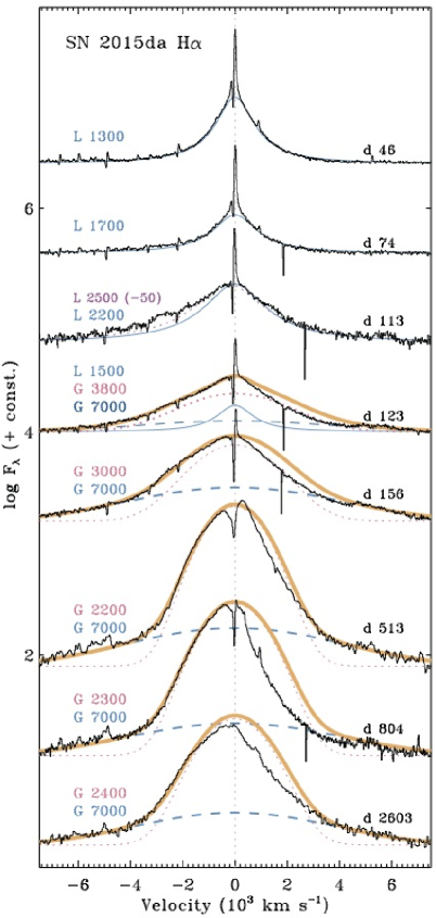
Figure 8: A series of observed spectra showing the H$\alpha$ line profile in SN 2015da (black), compared with smooth Lorentzian or Gaussian profile shapes (blue or magenta), and the sum of these (thick orange curve) when more than one is used. For day 113 we also plot a FWHM = 2500 km s^-1 Lorentzian that is shifted by $-$50 km s^-1 (purple dashed line). Each epoch lists the Lorentzian (L) or Gaussian (G) value(s) for the FWHM in km s^-1 to the left of the line. At later epochs, these curves intentionally ignore the red wing of the line, presuming that there is a deficit of flux in the red wings due to internal obscuration (see text).

3.5 H$\alpha$ profile fits and velocity

Here we explore functional approximations to the H$\alpha$ line shape and its evolution with time. Figure 8 shows a selection of observed H$\alpha$ profiles in our spectra (black) compared to Lorentzian or Gaussian functional shapes (or combinations of them).

As noted above, the first two epochs on days 46 and 74 have wings that are well matched by the shape of a symmetric Lorentzian function centred on zero velocity, while the narrow emission sits atop this Lorentzian. This is typical of SNe IIn at early times. Physically, this line shape is thought to arise when narrow-line photons from the slow pre-shock CSM must escape from high optical depths, and where thermal electron scattering broadens the profiles to the red and blue by the same amount (Chugai, 1977; Smith et al., 2008b). Lorentzian FWHM values of 1300 and 1700 km  s^-1 on days 46 and 74 (respectively) are typical of early SLSNe IIn spectra (Fransson et al., 2014; Smith et al., 2008b, 2010; Smith & Andrews, 2020; Dickinson et al., 2023). These Lorentzian shapes topped by narrow P Cygni emisson/absorption are reproduced in radiative-transfer simulations (Dessart et al., 2015).

Looking closely, a Lorentzian profile matches the line wings on day 46 in great detail, within the limits of S/N. By day 74, however, we can already see a small discrepancy between the observed line wings and the Lorentzian, with a slight excess of observed flux in the blue wing at $-$2000 to $-$4000 km s^-1. This excess is relatively small, but more than the noise. By day 113, right around the time of peak luminosity, a Lorentzian function centred at zero utterly fails to capture the shape of the observed line wings. A 2200 km s^-1 Lorentzian centred on the narrow emission on day 113 matches the red wing, but does not come close to matching the blue wing. Even a broader 2500 km s^-1 Lorentzian that has its centroid artificially shifted by $-$50 km s^-1 from the narrow emission (purple dashed line in Fig. 8) still underestimates the blue wing on day 113, although it comes closer than a centred Lorentzian. This discrepancy with Lorentzian profiles only worsens as time proceeds after day 113. For all epochs after day 113, we therefore use a combination of multiple Gaussian components to match the line shape.

Here our analysis differs significantly from that of SN 2015da’s spectra by T20. T20 interpreted the blueshifted H$\alpha$ emission profiles the same way that Fransson et al. (2014) interpreted the similar blueshifted profiles in SN 2010jl — as being due to broadening by electron scattering at all epochs, but where a symmetric Lorentzian function has its centroid shifted to the blue relative to the narrow emission at zero velocity. As noted by Smith & Andrews (2020), the physical basis for this idea is doubtful, since the Lorentzian shape of the electron-scattering wings must be symmetric about the source of the original narrow-line photons that get broadened by electron scattering. However, in this case of SN 2015da, and previous examples of SNe IIn that show a similar blueshift in their intermediate-width components, the narrow lines are not blueshifted by the same amount as the centroid of the putative Lorentzian function. Simulations also show line wings that are symmetric about zero velocity (i.e., the centroid of the narrow emission) until late times (around day 200 in the case of SN 2010jl) when the wings are influenced by the post-shock gas that becomes visible (Dessart et al., 2015). Here we therefore do not adopt this same unphysical picture of symmetric but artificially blueshifted Lorentzians.

Instead, a more plausible explanation for the asymmetry is that the line profiles appear asymmetric and blueshifted because some portion of the receding (redshifted) emission is blocked from our view. As noted by Smith et al. (2012) for the case of SN 2010jl, this may occur either through occultation by the SN ejecta photosphere (at early times) or by dust grains that have formed in the SN ejecta or shocked CSM (at later times).

The dust vs. electron-scattering interpretations of the blueshift are discussed more in Section 4; we would normally not mention the physical interpretation in this stage of the analysis, but in this case, the physical picture influences how we choose to measure velocities from the observed spectra. One specific quantity of prime interest that we wish to measure is the velocity of the forward shock running into the CSM. In T20’s approach, the lines are broadened by electron scattering, and so the observed line widths provide no information about the speed of the forward shock, because the width is not a kinematic width. In the interpretation where the intermediate-width emission arises from post-shock gas, but appears asymmetric because the far side is blocked by the photosphere or dust, accounting for this fact is important. If we want to derive the speed of the forward shock (which in SNe IIn is the same as the speed of the cold dense shell (CDS) that emits the intermediate-width component), then we wish to know the intrinsic FWHM of the line. However, if the redshifted emission is selectively blocked from our view, then the observed FWHM will clearly underestimate the true intrinsic speed. Instead, the HWHM of the blue side of the line is more indicative of the intrinsic width of the line before extinction shapes the line, because the approaching material is not blocked. In terms of simple functional approximations of the line shape, this is equivalent to fitting the blue wing of the line, and allowing the observed flux to fall below these curves on the red side or even at line centre.

We adopt this approach for functional fits to all spectra taken after the time of peak luminosity. Examples of the late-time spectra with multicomponent Gaussians are shown in Figure 8.

From day 123 onward, we could not find any Lorentzian (even with a shifted centre) that provided an acceptable match to the line shapes (although on day 123, there may still be some weak emission from a Lorentzian profile that contributes to the total line profile on top of the broad and intermediate-width Gaussians). After peak brightness, all epochs require at least two Gaussians to match the blue side of the profile. Because we suspect that dust blocks the red side, we used Gaussians that are centred on zero velocity, but we ignore the red wing. On the red side of the line, the difference between the functional profiles and the observed red wing clearly demonstrates the asymmetry, and indicates how much line flux is missing.

For each of the late-time spectra (day 123 onward), we found that a broad FWHM = 7000 km s^-1 Gaussian gave an adequate approximation of the broad wings, presumably due to emission from the fast SN ejecta. Note that well after day 100, the SN ejecta are no longer significantly heated by internal radioactivity. Instead, the fast emitting SN ejecta are probably heated as they approach the reverse shock by backwarming (see Smith et al., 2008b). In principle, this speed should decline over time, as the speed of ejecta that reach the reverse shock must decrease with time. However, the S/N of the fainter wings is not sufficient to accurately constrain this reduction in speed, so we use the same Gaussian FWHM for all epochs. This is not an accurate sampling of the SN ejecta speed, but is needed to provide a broad base for fitting the intermediate-width components.

Importantly, however, the observed broad wings are not asymmetric. We matched the broad 7000 km s^-1 Gaussian curves to the blue wings, but they also match the observed flux on the red wing beyond velocities of about $+$4000 or $+$5000 km s^-1. This is important, because it indicates that at later epochs, the emission from the receding fast SN ejecta does not suffer the same obscuring effects as the emission from the post-shock CDS that emits the intermediate-width component. This is an important clue to the location of the obscuring material, and we return to it later.

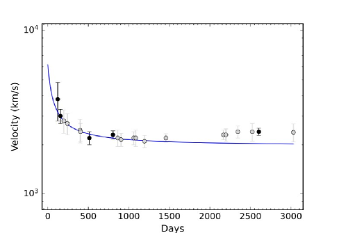
Figure 9: The speed of the forward shock as a function of time inferred from spectra. Measurements correspond to the FWHM of the intermediate-width Gaussian components in Figure 8, which are only matched to the blue sides of the lines (these are equivalent to 2 times the HWHM values for the blue wings). The blue curve is a smoothly dropping velocity that we use to approximate the CDS velocity later in our analysis, and this curve intentionally ignores the rise in apparent velocity after day 2000 (see text).

3.6 Speed of the forward shock

After the time of peak brightness, the intermediate-width components are tracing emission from the CDS, and therefore can provide an estimate of the important value for the speed of the forward shock running into the CSM. Figure 8 shows how we estimated these FWHM values for several representative epochs (these correspond to the Gaussian FWHM values listed in magenta and shown by a dotted magenta curve in the plot). These FWHM values are approximate, since we are matching the profile shape mainly to the blue wing, as the red wing may be missing due to extinction. Uncertainties in these FWHM values are typically 100–300 km s^-1, depending on the data quality, the irregularity of the shape, and in some cases the uncertain overlap with the broad component.

Although Fig. 8 shows only a few examples, we measured this intermediate-component FWHM in all of our spectra. Fig. 9 plots the resulting FWHM velocities of the intermediate-width components in our spectra from day 156 onward, after the intermediate-width profiles are no longer dominated by Lorentzian profiles. The blue curve in Fig. 9 is a simple smoothly declining velocity passing through these data, approximating the speed of the CDS that decelerates as it gets mass-loaded with CSM. This is used later in our analysis.

Curiously, Fig. 9 shows that the line width increases slightly again after day 1500, rising from a minimum of 2100 km s^-1 around day 1200 up to 2400 km s^-1 in our last epoch around day 3030. There are two potential explanations for this, but it is difficult to determine which is correct. First, it could mean that the speed of the CDS is actually accelerating. By $\sim$1200 days, SN 2015da may have completely outrun its dense shell of CSM. Continuing to expand into a rarefied medium, the CDS would still be pushed by the fast SN ejecta hitting the reverse shock, so the shock might accelerate outward through the dropping density gradient. SN ejecta hitting the reverse shock still have a speed of 7000 km s^-1 at that time. A second possible explanation is observational; as the intermediate-width component gets fainter, it becomes somewhat blended with emission from the SN ejecta and reverse shock, and the contribution of some broader emission may widen the intermediate-width component. This is the first time to our knowledge that the intermediate-width emission component has been seen to broaden at late times. In any case, the blue curve in Fig. 9 ignores this late increase.

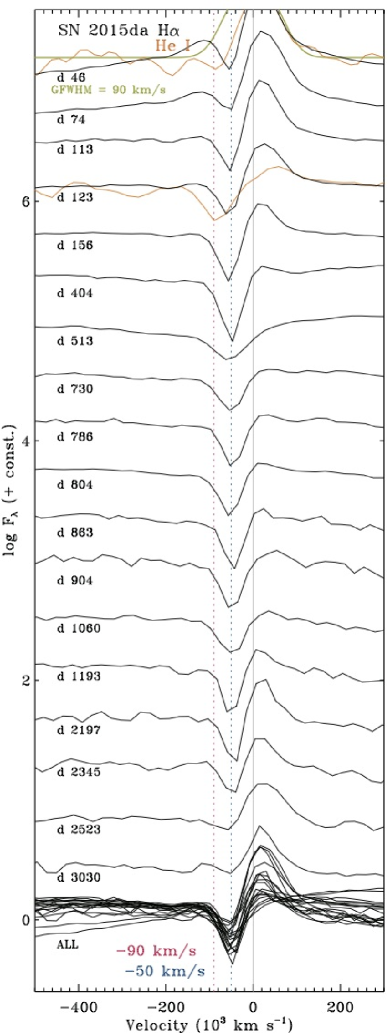
Figure 10: Evolution of the line profile for the narrow P Cygni component of H$\alpha$ (black), tracing the expansion of the unshocked CSM. For days 46 and 123, we show the same profiles of He i $\lambda$5876 (in orange) that were plotted in the right panel of Figure 4, for comparison, as well as the same FWHM = 90 km s^-1 from that figure (in lime green). The vertical dotted lines in magenta and blue show reference values of $-$90 km s^-1 and $-$50 km s^-1, respectively. $-$50 km s^-1 roughly matches the trough of the P Cygni absorption of H$\alpha$, whereas $-$90 km s^-1 approximately matches the trough of the P Cygni absorption of He i and the blue edge of the P Cygni absorption in H$\alpha$. At the bottom, all the H$\alpha$ profiles in the figure are overplotted together with no vertical offset.

3.7 Narrow components from CSM

In SNe IIn, the namesake narrow emission components provide important information about the pre-shock CSM, and hence, valuable information about the pre-SN state of the progenitor star. Above (see Fig. 4), we already mentioned that He i $\lambda$5876 shows a narrow emission component and a P Cygni absorption component at $-$90 km s^-1. That He i line is clearly detected in only two of our spectra (days 46 and 123). Here we consider the narrow component of H$\alpha$ and its evolution over time. Figure 10 shows a sequence of spectra that focuses on the narrow component of H$\alpha$ as seen in some of our spectra with relatively high resolution and good S/N, and the two epochs where He i is detected are overplotted in orange.

From Figure 10, it is clear that while the strength of narrow H$\alpha$ emission and P Cygni absorption fluctuates, the width of the emission and the velocity of the P Cygni absorption are remarkably steady. The minimum of the P Cygni absorption trough is at roughly $-$50 km s^-1 (vertical blue dotted line) from our first epoch to the last. The blue edge of the P Cygni absorption is at roughly $-$90 km s^-1 (vertical magenta dotted line), although this blue-edge velocity does seem to fluctuate more than the velocity of the absorption minimum, perhaps in part because the underlying intermediate-width emission component is varying as well. In the first spectrum on day 46, when the narrow emission component is strongest, we show the same FWHM = 90 km s^-1 Gaussian profile from Fig. 4 (in lime green). That Gaussian was found to capture the emission profile of the He i line quite well (accounting for the fact that the blue side of the line is absorbed), and this appears to match the width of H$\alpha$. From this, and the blue edge of the H$\alpha$ P Cygni absorption, we therefore adopt a constant CSM expansion speed of 90 km s^-1 in our analysis below.

A caveat is in order, since this inferred expansion speed of 90 km s^-1 is dangerously close to the resolution at H$\alpha$ in these spectra, which is $\sim$70 km s^-1. These narrow profiles are therefore underresolved. When higher-resolution echelle spectra are available for other SNe IIn, as in the case of SN 2017hcc (Smith & Andrews, 2020), we find that our 1200 lines mm^-1 grating spectra with MMT/Bluechannel do miss some important information about the line shape. The blue edge and transition from absorption to emission are likely sharper than shown in these data, so an uncertainty of 15–20 km s^-1 is likely for the inferred velocity. Nevertheless, the spectra in Figure 10 do not show a systematic gradual increase or decrease in the velocity of the P Cygni absorption, so the conjecture of a relatively constant expansion velocity in the CSM ahead of the shock is probably correct.

A constant CSM speed has important physical implications. SN 2015da was extremely luminous, and it sustained a high luminosity for an unusually long time compared to most SLSNe IIn, requiring a relatively large radial extent in the dense CSM. A constant CSM expansion speed suggests that the very strong pre-SN mass loss was in the form of a very strong but sustained steady wind or a long series of many similar episodic events, rather than a single short-duration burst of mass loss. A sudden pre-SN outburst or explosion would likely lead to a Hubble-like flow in the CSM, where expansion speed is proportional to distance from the star, translating to an increase in the observed outflow speed in later spectra. A clear sign of a relatively sudden burst of mass loss 8 yr before the SN was seen in similar data for SN 2006gy (Smith et al., 2010), so SN 2015da offers an interesting counterpoint showing a constant-speed wind.

The $\sim$90 km s^-1 outflow speed is seen in all our spectra until at least 3000 days after explosion. This provides an important constraint on the minimum duration of pre-SN mass loss, assuming constant expansion speed. The time it took for the progenitor to create the dense CSM is $t_{\rm CSM}=t_{\rm SN}\times V_{\rm SN}/V_{\rm CSM}$, where $t_{\rm SN}$ is the time of observation since the SN exploded, $V_{\rm SN}$ is the speed of the forward shock, and $V_{\rm CSM}$ is the expansion speed of the CSM. With a forward shock expanding at roughly 2100 km s^-1 (this is the minimum speed; see above), this translates to a strong pre-SN wind that lasted for at least 160 yr before core collapse. Given the higher $V_{\rm SN}$ speeds during the earlier parts of the light curve (Fig. 9), 200 yr is a better estimate. This length of time helps to clearly rule out some mechanisms, like wave driving, as the culprit for the pre-SN mass loss, since wave driving can only operate effectively on timescales of around 1 yr before core collapse, as noted in the Introduction. Some other mechanism(s) must be responsible for the extreme mass loss by SN 2015da’s progenitor.

Finally, it is interesting to note that while the widths of emission components agree for H$\alpha$ and He i, the He i P Cygni absorption seems to indicate higher expansion speeds than H$\alpha$. This is most clear on day 123 in Figure 10, where the P Cygni minima of He i and H$\alpha$ are at $-$90 and $-$50 km s^-1 (respectively), and the blue edge of He i absorption extends to $-$160 km s^-1, almost double that of H$\alpha$.

Curiously, the situation is exactly the opposite of what was seen recently in SN 2017hcc, which is another SLSN IIn. In SN 2017hcc, the widths of emission components agreed for H and He lines, as is the case here, but the disagreement in absorption velocities was flipped: in SN 2017hcc, the H Balmer lines showed faster velocities in the P Cygni absorption, and the He i P Cygni absorption had slower expansion velocities (Smith & Andrews, 2020). This was attributed to geometric effects, where the velocity and excitation level are latitude dependent when an asymmetric disk-like CSM geometry is hit by the SN. Since SN 2015da also has asymmetric CSM (see below), and since this effect depends on viewing angle, this could signify that SN 2015da is viewed from a substantially different latitude than SN 2017hcc. The fact that the H/He velocity disagreement is flipped in these two SLSNe argues for a geometric viewing-angle effect rather than an alternative explanation where pre-shock acceleration has a stronger influence on higher-ionisation lines. If the correct explanation were the latter, we should expect the physics to work the same way in both objects.

4 Discussion

4.1 Asymmetry

SN 2015da is remarkable both in its high peak luminosity that makes it an SLSN IIn, and in how it sustained such a high luminosity over time. This is even more remarkable when we consider evidence that the CSM is asymmetric, since asymmetry tends to reduce the global efficiency of converting kinetic energy into light, simply because asymmetric CSM intercepts only a fraction of the available ejecta.

Earlier we noted a few clues that the CSM interaction in SN 2015da is likely to be asymmetric. The most important clue is that we see the fast SN ejecta directly, even at early times. We see very broad emission wings in the H$\alpha$ emission-line profiles; moreover, low-resolution spectra reveal broad emission from the Ca ii near-IR triplet that is usually attributed to the fast SN ejecta, and in this case shows no intermediate-width or narrow emission components at these early times. These are seen around the time of peak luminosity and afterward. In addition, very broad P Cygni absorption is detected in He i $\lambda$5876 out to $-$10,000 km s^-1. A hint of this broad absorption is already present in the day 46 spectrum, and is clearly present by day 74 and afterward (see Fig. 4). Thus, we are already seeing direct emission and absorption from the fast, freely expanding SN ejecta, before the time of peak $R$-band luminosity. This is not possible in a spherical model for an SLSN, where the photosphere is still ahead of the shock in the pre-shock CSM at these phases (Dessart et al., 2015; Smith et al., 2008b; Woosley et al., 2007). Seeing the SN ejecta directly at such an early epoch requires that along some lines of sight to the SN ejecta, the optical depth is lower than required for other directions through the opaque CSM interaction region. This requires asymmetric CSM.

In fact, clear evidence for significant asymmetry in SN 2015da is provided by spectropolarimetry. Bilinski et al. (2023) presented multi-epoch spectropolarimetry of SN 2015da taken at early epochs up to and around the time of the main luminosity peak. During this phase SN 2015da showed a continuum polarization of $\sim 3$%, which is on the high side for SNe IIn and indicates a significant degree of asymmetry.

If the CSM of SN 2015da is significantly asymmetric, then this is important to keep in mind when evaluating the global energy budget of the event discussed in the next section. When CSM interaction is the dominant power source for a bright SN, some fraction ($f$) of the available kinetic energy of ejecta reaching the shock (i.e., the explosion kinetic energy, $E_{\rm exp}$) is converted to light, and so the integrated radiated energy that we observe ($E_{\rm rad}$) is obviously only a lower limit to the explosion energy: $E_{\rm exp}\geq E_{\rm rad}/f$. For simulations of SLSNe with spherical CSM interaction, $f$ can be quite high (i.e., 0.3 to 0.5, for example; van Marle et al. 2010). Now suppose that the CSM is asymmetric, and that the CSM intercepts only some fraction $q$ of the $4\pi$ steradians of the explosion. For a thick disk or the waist of a bipolar CSM shell, $q$ might plausibly be 0.1–0.4. If the asymmetric CSM can only tap into a fraction of the available kinetic energy, then some of the ejecta expand without experiencing strong interaction; thus, $E_{\rm exp}\geq E_{\rm rad}/fq$. With both correction factors $f$ and $q$, if the CSM is asymmetric, we can easily have $E_{\rm exp}\approx(5-10)\times E_{\rm rad}$ (and of course, note that these correction factors are in addition to any bolometric correction that should already have been applied to $E_{\rm rad}$, if $E_{\rm rad}$ is derived from optical photometry, and they do not account for interior SN ejecta that have yet to reach the reverse shock). This geometric efficiency factor is significant, since SN 2015da is already a very energetic event before correction. A similar correction to the inferred energy was discussed previously regarding the asymmetry in SN 2009ip (Mauerhan et al., 2014; Smith, 2014), but in that case the total required explosion energy was corrected from around $10^{50}$ erg up to $10^{51}$ erg. In the case of an SLSN IIn like SN 2015da, this correction pushes the limits more because, as we discuss below, the observed value of $E_{\rm rad}$ already exceeds the canonical SN explosion energy of $10^{51}$ erg.

4.2 CSM interaction: mass and energy budget

Earlier in Section 3.2, from the $R/r$-band light curve of SN 2015da, we measured a value for the total integrated radiated energy of $E_{\rm rad}=1.6\times 10^{51}$ erg. We estimated a somewhat higher value of $E_{\rm rad}=1.9\times 10^{51}$ erg if we adopted the “pseudo-bolometric” correction from T20. When we consider the likely correction factors $f$ and $q$ for the conversion efficiency and asymmetric geometry, respectively, the value of $E_{\rm exp}>E_{\rm rad}/fq$ quickly climbs to around (5–10) $\times 10^{51}$ erg. Thus, just from the radiated energy budget generated by CSM interaction, we already have important constraints on the explosion, because this is too much for any SN Ia, and it is on the high end for normal core-collapse SNe. However, even this is still a lower limit to the required explosion energy, because we must also account for the kinetic energy in the SN ejecta that have not yet reached the reverse shock, and the kinetic energy due to the final coasting speed and swept-up mass in the post-shock shell. The former is difficult to estimate, requiring models to infer the mass and speed of ejecta that have not yet reached the reverse shock by $\sim$2600 days. However, observations do allow good constraints on the mass and kinetic energy of the post-shock shell.

When CSM interaction dominates the observed luminosity, as is thought to be the case in SLSNe IIn, the luminosity can be used to infer the density of the CSM and the progenitor’s mass-loss rate using the relation Smith (2017)

$$L=\frac{1}{2}wV_{\rm SN}^{3}=\frac{\dot{M}V_{\rm SN}^{3}}{2V_{\rm CSM}}\,,$$ (1)

where $w$ is the wind density parameter $w=4\pi R^{2}\rho$ or $w=\dot{M}/V_{\rm CSM}$, $\dot{M}$ is the progenitor star’s mass-loss rate, and $V_{\rm SN}=V_{\rm CDS}$ is the speed of the forward shock, indicated by the observed speed of the CDS. Here, $L$ is the luminosity generated by CSM interaction; this luminosity might be greater than the observed optical luminosity $L_{\rm opt}$ (or even the pseudo-bolometric luminosity), if some significant portion of the radiated energy escapes as X-rays, for example. In the case of SLSNe IIn, we generally assume that $L\approx L_{\rm opt}$ at early times during the main light-curve peak when X-rays are absorbed and thermalised (Smith & McCray, 2007), but this becomes an increasingly risky assumption at later times, when the optical depth drops and significant X-ray flux can escape. Thus, once again, one should be mindful of another correction factor that acts to raise the mass and energy budget even more.

We adopt a constant value of 90 km s^-1 for $V_{\rm CSM}$, based on the steady narrow P Cygni absorption seen throughout the evolution of SN 2015da (Fig. 10). The value for the speed at which the shock sweeps into the CSM, $V_{\rm SN}=V_{\rm CDS}$, is provided observationally by the line width of emission from the post-shock gas in the CDS. This is indicated by the intermediate-width components of emission lines, but only after their transition from Lorentzian profiles (dominated by electron scattering in the CSM) to the profiles after peak that trace expansion of post-shock gas. As noted earlier, the red wings of these emission lines suffer selective velocity-dependent extinction, probably from internal dust formation (see below), so the value of $V_{\rm CDS}$ is best indicated by 2 times the blue HWHM velocity, or the FWHM of symmetric Gaussians that are only fit to the blue wing. The value of $V_{\rm CDS}$ is time dependent, because the shock decelerates over time as it gets mass loaded. As noted earlier, observed estimates of this velocity are plotted in Fig. 9. The value of $V_{\rm SN}=V_{\rm CDS}$ that we adopt at each time step is given by the smooth blue curve in Fig. 9.

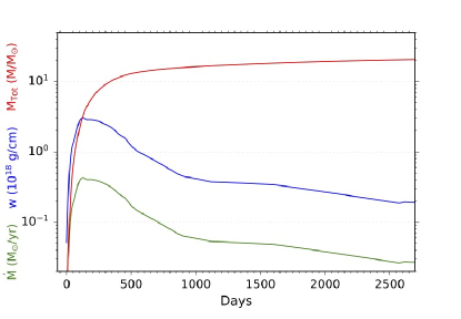
Figure 11: Values for the progenitor mass-loss rate (green), the wind density parameter $w$ (blue), and the cumulative mass swept up by the shock $M_{\rm Tot}$ (red) as a function of observed time since explosion. These are derived from the observed luminosity and the CSM and shock speeds (see text).

With observed estimates for $L$, $V_{\rm SN}$, and $V_{\rm CSM}$, we can calculate the characteristic wind density parameter and progenitor mass-loss rate corresponding to the CSM overtaken by the shock, given by

$$\dot{M}=wV_{\rm CSM}=2\ L\ \frac{V_{\rm CSM}}{(V_{\rm SN})^{3}}\,,$$ (2)

at each time step. Calculated values for $w$ and $\dot{M}$ at each time are plotted in blue and green (respectively) in Figure 11. The time in days on the horizontal axis is the time since the SN exploded, $t_{\rm SN}$. As noted in Section 3.7, this can be converted to the timescale it took the progenitor to make the CSM via $t_{\rm CSM}=t_{\rm SN}\times V_{\rm SN}/V_{\rm CSM}$. The red curve, $M_{\rm Tot}$, shows the cumulative amount of CSM mass that has been swept up by the shock at each time step; it is the integral of $\dot{M}\times\Delta t_{\rm CSM}$.

From Figure 11 we see that SN 2015da requires at least 20 $M_{\odot}$ of swept-up CSM. It therefore joins some of the most extreme SLSNe IIn like SN 2006gy, SN 2006tf, SN 2003ma, and SN 2016aps, which require similar amounts of CSM (Smith & McCray, 2007; Smith et al., 2008b, 2010; Woosley et al., 2007; Rest et al., 2011; Nicholl et al., 2020). Normally, one must be cautious with interpreting a value for $\dot{M}$ because the pre-SN mass loss can be more explosive than steady, but in this case of SN 2015da, we observe a steady CSM expansion speed of 90 km s^-1 throughout its evolution. This indicates that the progenitor was losing material at a relatively steady (but astonishing) rate of $\sim 0.4$ M_⊙ yr^-1 for several decades before explosion, and at a somewhat less extreme rate of $\sim 0.04$ M_⊙ yr^-1 for another 2 centuries before that.

The final coasting speed of the swept-up CDS also places important constraints on the mass of SN ejecta, since the SN ejecta must provide not only the energy needed for the SN luminosity, but also the momentum imparted to the accelerated CSM. From simple momentum conservation, we have the constraint

$$M_{\rm e}=M_{\rm CSM}\frac{(V_{\rm CDS}-V_{\rm CSM})}{(V_{\rm e}-V_{\rm CDS})}\,,$$ (3)

where, as before, $V_{\rm CDS}$ is the observed speed of the post-shock CDS, and $M_{\rm CSM}$ and $V_{\rm CSM}$ are the mass and speed of the pre-SN CSM. Also, $V_{\rm e}$ is the effective velocity of the SN ejecta, and $M_{\rm e}$ is the mass of SN ejecta that has hit the reverse shock. Since ejecta with $V_{\rm e}<V_{\rm CDS}$ have not yet contributed their momentum to the CDS, $M_{\rm e}$ is a lower limit to the required total SN ejecta mass. Observations noted above provide values of $M_{\rm CSM}=20$ M_⊙, $V_{\rm CDS}\geq 2100$ km s^-1, and $V_{\rm CSM}=90$ km s^-1. We do not know $V_{\rm e}$ a priori, but for a typical SN Ia, the velocity $\sqrt{2E/M}$ is about 8500 km s^-1. These values would then require SN ejecta mass of $M_{\rm e}>6.5$ M_⊙. This clearly rules out any SN Ia scenario for SN 2015da, which is in good agreement with the total CSM mass budget exceeding 20 M_⊙ and the total energy well above $10^{51}$ erg, both of which also rule out any model involving SNe Ia.

What mechanism powers the extreme pre-SN mass loss? As noted earlier, the timescale of a few centuries before explosion rules out wave driving as the source, since this only works on timescales around 1 yr (Quataert & Shiode, 2012; Shiode & Quataert, 2014; Fuller, 2017). Recent work also suggest that this mechanism may inject less power into the envelope than previously thought, and may favour lower-mass progenitors (Wu & Fuller, 2021), exacerbating the difficulty for this mechanism to explain SLSN IIn precursor mass loss.

The only remaining proposed mechanisms for extreme pre-SN mass loss include the pulsational pair instability or other nuclear burning instabilities (Woosley et al., 2007; Woosley, 2017; Smith & Arnett, 2014; Arnett & Meakin, 2011; Renzo et al., 2020), or pre-SN binary interaction (Smith & Arnett, 2014; Schrøder et al., 2020; Fryer & Woosley, 1998).

Of these, pulsational pair instability is the mechanism with the most clear and well-established predictions. This mechanism seems well suited to account for the inferred CSM mass, the energy budget of the pre-SN mass loss, and potentially the timescale for the pre-SN mass-loss. While the pulsational pair instability generally occurs during O burning — which, like wave driving, usually only occurs around 1 yr before death — the energetic pulses instigated by explosive O burning can expand the core, which relaxes on a long thermal timescale. As such, extreme mass loss can potentially occur for many decades or even centuries before the star finally dies (Woosley, 2017). However, the fact that the strong mass loss from pulsational pair instability occurs via a series of hydrodynamic pulses means that it is driven off the star by shocks, and thus results in fast expansion speeds. The bulk expansion speeds of the ejecta are always around 2000 km s^-1 or larger (Woosley, 2017; Renzo et al., 2020; Woosley & Smith, 2022). Moreover, the first pulse generally removes the residual H envelope, with the subsequent ejecta being H poor (Renzo et al., 2020; Woosley & Smith, 2022). These are robust predictions, and they strongly disfavour pulsational pair instability as the trigger for the strong pre-SN mass loss in SN 2015da. This is because SN 2015da showed a remarkably steady CSM expansion speed of only 90 km s^-1 for centuries before explosion, and always exhibited strong H lines, even in the broad lines from the freely expanding SN ejecta. This is difficult to achieve with a series of strong pulses that suddenly eject the star’s H envelope. The observational expectations for other nuclear burning instabilities are not as clear as for the pulsational pair instability, so further work on these is warranted. Since the energy is deposited deep inside the star and should steepen to a shock as it approaches the surface (Fuller & Ro, 2018), the observational consequences might be similar to those of the pulsational pair instability.

On the other hand, a slow and steady expansion speed of around 90 km s^-1 over centuries may be well suited to the slow leaking of mass that must occur during the relatively long inspiral phase before a merger event. This roughly matches the $\sim$100 km s^-1 pre-eruption mass loss seen in light-echo spectra of $\eta$ Carinae before its merger (Smith et al., 2018), which also produced a CSM mass of order 20 M_⊙ (Smith et al., 2003a). Moreover, the fact that the pre-explosion mass loss inferred for SN 2015da ramps up with time (see Fig. 11) also agrees well with a merger scenario. The total expansion kinetic energy of the CSM ($0.5\times 20$ M${}_{\odot}\times$ (90 km s^-1)²) is around $2\times 10^{48}$ erg, which is easily supplied by the available orbital energy in a massive-star merger. So far, some sort of pre-SN merger event (Smith & Arnett, 2014) seems like the most favourable explanation for providing the astounding pre-SN mass loss for SN 2015da. We note that while the pre-SN mass loss of SLSNe IIn closely resembles the strong mass loss of LBVs (Smith et al., 2007), it is quite possible that most giant eruptions of LBVs are themselves stellar merger events, as is thought to be the case for $\eta$ Carinae (Smith et al., 2018). The reason a merger might occur immediately before a very energetic SN explosion is still unclear, however. Perhaps late burning phases cause the star to swell, synchronising the binary interaction with core collapse (Smith & Arnett, 2014), or perhaps a merger with a compact companion triggers a violent energetic explosion powered by accretion (Fryer & Woosley, 1998; Schrøder et al., 2020; Smith & Arnett, 2014). Further theoretical exploration in this direction (including the predicted observational signatures) is certainly worthwhile.

4.3 Blueshifted line profiles and dust

SN 2015da also joins a number of well-observed SLSNe IIn and SNe IIn that exhibit asymmetric blueshifted profiles in their intermediate-width emission lines from the post-shock CDS. Other well-studied examples include SN 2017hcc (Smith & Andrews, 2020), ASASSN 15ua (Dickinson et al., 2023), KISS15s (Kokubo et al., 2019), SN 2013L (Andrews et al., 2017), SN 2010jl (Smith et al., 2012; Gall et al., 2014), SN 2010bt (Elias-Rosa et al., 2018), SN 2007rt (Trundle et al., 2009), SN 2007od (Andrews et al., 2010), SN 2006tf (Smith et al., 2008b), SN 2005ip (Smith et al., 2009b; Fox et al., 2010; Smith et al., 2017), and SN 1998S (Mauerhan & Smith, 2012; Pozzo et al., 2004). This blueshift is also seen clearly in some interacting H-poor SNe, most notably in SN 2006jc (Smith et al., 2008a).

In most interacting SNe that show these blueshifted line profiles, the lines begin symmetric (usually with Lorentzian-shaped profiles) and evolve to become blueshifted over time. This, and the narrow lines centred on zero velocity, argue against a pervasive tendency for SN IIn progenitors to launch one-sided CSM preferentially toward Earth. Instead, it is more likely that something within the SN explosion is blocking the redshifted portions of the emitting material.

The most common explanation for the observed systematic blueshift in emission-line profiles in interacting SNe is that new dust grains are forming, either in the SN ejecta or in the dense rapidly cooling post-shock CDS. Only dust that is found internal to the SN (i.e., not circumstellar) can preferentially block the receding material, simply because the emission from the far side has a long path length passing through the explosion interior, whereas the blueshifted emission does not. This effect was most famously seen in SN 1987A, where developing blueshifted line profiles from SN ejecta were accompanied by an increased rate of fading and by growing IR excess emission (Danziger et al., 1989; Lucy et al., 1989; Gehrz & Ney, 1990; Wooden et al., 1993; Colgan et al., 1994). Models of the line-profile evolution indicate continual growth of dust grains for decades in SN 1987A (Bevan & Barlow, 2016).

Each of these observational effects — increased rate of fading, excess IR emission, and blueshifted line profiles — taken on their own might be ambiguous, because there may be more than one cause for each. But when all three developments occur together, as in SN 1987A, it presents a strong case that new dust grains are forming in the SN. The first interacting SN to clearly show all three signs was SN 2006jc (Smith et al., 2008a), which also exhibited an outburst in X-ray emission (Immler et al., 2008) accompanied by He ii $\lambda$4686 emission at the same time. This coincidence, the early onset of these effects at $\sim$50 days, and the fact that the intermediate-width He i lines showed a deficit of flux at zero velocity as well as on the red wing, indicated clearly that the location of the newly formed dust was in the post-shock region within the CDS, and not in the fast SN ejecta. Smith et al. (2008a) noted that this is quite similar to the episodic post-shock dust formation that occurs in eccentric colliding-wind binaries like WR 140 (Hackwell et al., 1979; Williams et al., 1990; Monnier et al., 2002) and $\eta$ Car (Smith, 2010), where episodes of post-shock dust formation at periastron are accompanied by strengthening X-ray emission and He ii $\lambda$4686 emission from the shock.

In SNe IIn, the late-time luminosity is typically dominated by ongoing CSM interaction rather than radioactive decay, so unfortunately, it is difficult to tell if there is an increased rate of fading from additional extinction (because we don’t really know the intrinsic luminosity decline rate, as we do for ⁵⁶Co decay). As such, we are left with the two remaining indicators of dust formation: IR excess emission and blueshifted line profiles.

Mid-IR excess emission from dust is seen in every example mentioned above where SNe IIn or Ibn show blueshifted line profiles (when mid-IR observations were obtained). From an IR excess alone, however, it is unclear where the dust is located or if it is new. It could be formed in the SN ejecta or in the post-shock CDS, but in principle the dust might also be pre-existing and could be seen as an IR echo (Gerardy et al., 2002). This echo could be a true echo where CSM dust is heated by the main peak of light curve, or a continual echo where luminosity from ongoing CSM interaction heats CSM dust just ahead of shock. In fact, regardless of whether new dust forms in the SN, it is likely for any SN IIn to have an IR echo, since the very dense and slow CSM that is required to make it appear as an SN IIn is also likely to be dusty. The IR excess emission in both SN 2010jl (Andrews et al., 2011; Sarangi et al., 2018) and SN 2015da (T20) were interpreted as IR echoes. Most SNe IIn show continually re-heated IR echoes from ongoing late-time CSM interaction (Fox et al., 2013). The presence of an IR echo does not, of course, preclude the possibility that new dust also forms in the SN.

As noted above, several SNe IIn have shown clear evidence for a net blueshift in the centroid of emission lines, and in many cases, an asymmetric skewed line-profile shape. As in the case of SN 2006jc, the specific velocity components of the lines that show the blueshift, plus the detailed shape of the line, can help us decipher the region where new dust must be forming. In SN 1987A, the blueshift was seen in the broad emission lines from the freely expanding SN ejecta. In SNe IIn and Ibn, the blueshift is sometimes seen in the broad ejecta components, but is more commonly seen in the intermediate-width components emitted by the post-shock gas (Smith et al., 2009b, 2012; Gall et al., 2014; Smith & Andrews, 2020). Modeling of the line profiles in SNe IIn has confirmed that dust formation in the ejecta or post-shock regions (or sometimes both) can account for the observed line profiles, and models can disentangle the relative amount in each region (Chugai, 2018; Bevan et al., 2019, 2020). Dust that forms only in the SN ejecta can block the red wings of both the broad components and potentially the intermediate-width component, since the most redshifted portion of the CDS may be behind the inner SN ejecta. However, dust in the inner SN ejecta cannot block emission from the CDS at around zero velocity, since this material is moving in the plane of the sky and is outside the SN ejecta; when intermediate-width components show a deficit of emission in both the red wings and around zero velocity, this requires dust in the CDS (Smith et al., 2008a, 2012; Chugai, 2018).

SN 2015da presents another case of an SLSN IIn that clearly showed both the IR excess from warm dust and blueshifted emission-line profiles. T20 interpreted the IR excess and the blueshifted profiles as separate phenomena: the IR excess was attributed to an IR echo from pre-existing CSM dust, as noted above, whereas the pronounced blueshift was attributed to the same scenario proposed for SN 2010jl by Fransson et al. (2014). Fransson et al. (2014) attributed the blueshifted profiles in SN 2010jl at all epochs to electron scattering of emission from pre-shock asymmetric CSM gas that was mostly on our side of the SN, and was accelerated toward the observer by radiation from the SN shock, thus producing intermediate-width lines with a symmetric shape, but with a centroid offset from zero velocity. As discussed in detail by Smith & Andrews (2020), however, there are three key reasons why the model proposed by Fransson et al. (2014) and adopted by T20 does not work. (1) the narrow emission components from the unshocked CSM are in fact detected, but they are not blueshifted, and they are not at the centre of the blueshifted intermediate-width component. Moreover, the narrow components show narrow P Cygni profiles that indicate the same slow velocities as the narrow emission. This means that the CSM has not been accelerated toward us, and that the blueshifted intermediate-width components cannot result from broadening of the observed narrow emission. (2) Although acceleration of pre-shock CSM may occur, the observed amount of a few hundred km s^-1 is too large (Dessart et al., 2015). Moreover, any radiative acceleration of CSM should be strongest when the SN luminosity is the highest (i.e., at peak), and should diminish at late times when the luminosity falls. But observations show the opposite, where the blueshift persists until late times and becomes even more pronounced with time after peak. (3) Similarly, the hypothesis where electron scattering dominates the line broadening requires high electron scattering optical depths, and this is expected to diminish with time as the SN fades and the electron-scattering opacity drops. But instead, the intermediate-width components tend to become even more blueshifted as the continuum opacity disappears, ruling out the electron-scattering model. Surely electron scattering does broaden the wings at early times when the lines are symmetric Lorentzians, but it cannot account for the asymmetric blueshifted profiles at late times.

A possible alternative cause of blueshifted profiles is that the continuum photosphere in the SN itself, rather than dust, blocks some of the redshifted emission. This was discussed in the context of the blueshifted profiles in SN 2010jl by Smith et al. (2012), who noted that as the SN fades and the continuum photosphere transitions to optically thin CSM interaction, this effect ceases to work and the line profiles should become symmetric again. In SN 2015da and previous examples like SN 2010jl and SN 2017hcc, observations show the blueshift persisting until very late phases more than 1000 days after explosion. Thus, while this occultation by the SN photosphere may help explain some of the early blueshift, it cannot explain the evolution after peak, so dust formation is required.

Besides the IR excess and the blueshifted profiles, there is one additional tell-tale sign of dust formation within the SN. When the blueshifted line profiles are seen, they may also exhibit a wavelength dependence, with stronger blueshifted asymmetry at shorter wavelengths. For example, compared to the asymmetric blueshifted profile seen in H$\alpha$, H$\beta$ might show even more blueshift, whereas a near-IR line like Pa$\beta$ might have a more symmetric profile. If this effect is seen, it leaves little doubt that new dust formation is the culprit behind the blueshifted profiles, because dust causes greater extinction at shorter wavelengths, whereas electron-scattering opacity is wavelength independent. Such wavelength dependence to the blueshift is indeed observed in some SLSNe IIn when good multiwavelength data are available, as seen clearly in both SN 2010jl (Smith et al., 2012; Maeda et al., 2013; Gall et al., 2014) and SN 2017hcc (Smith & Andrews, 2020). These cases indicate the rapid formation of relatively large grains (Gall et al., 2014; Smith & Andrews, 2020). This evidence requires either IR spectra with good S/N, or blue spectra covering H$\beta$ with very high S/N (H$\beta$ is much fainter than H$\alpha$ in interacting SNe at late times).

Considering all these points above, we find that in SN 2015da — as in the previous cases of SN 0210jl and SN 2017hcc — it is clear that the observed asymmetric blueshifted profiles arise because of copious new dust formation in the post-shock CDS. For the first few epochs leading up to the time of peak luminosity, the intermediate-width profiles of H$\alpha$ are indeed Lorentzian in shape and symmetric, centred on zero velocity. After peak, however, when the blueshift becomes strong, the line wings are no longer Lorentzian in shape. They become complex asymmetric blueshifted profiles, with centroids that are not just offset from zero velocity, but also profiles skewed in shape and multicomponent. The centroids of the intermediate-width components are shifted to the blue and offset from the narrow lines, which remain close to zero. This offset of the centroid of the intermediate-width component without any similar offset in the velocity of the narrow component definitively rules out electron scattering of radiatively accelerated CSM as the explanation for the profiles. Additionally, the blueshift becomes more pronounced as the SN fades, and remains strong until late times. This is the opposite of expectations for electron scattering and radiative acceleration, but it is expected for dust, which continues to form as the material expands and cools (Gall et al., 2014; Li et al., 2022), and where dust opacity remains high even at low temperatures.

While we were not able to obtain high-quality IR spectra of SN 2015da, we do see evidence for some wavelength dependence to the blueshift. We only have a few epochs of spectra with broad wavelength coverage that includes H$\beta$ (see Fig. 3), and in many of these, the S/N around H$\beta$ and the presence of other emission lines complicates a comparison. But in our last epoch obtained with the LBT, H$\beta$ is detected with good S/N; this profile is shown as a blue dashed curve at the bottom of Figure 7. When we adjust the flux so that the blue wings of H$\beta$ and H$\alpha$ match, there is clearly an additional deficit of flux on the red side of H$\beta$ as compared with H$\alpha$, even though H$\alpha$ is itself already blueshifted and asymmetric. The difference between H$\beta$ and H$\alpha$ at this epoch is similar to the differences between these two lines at late times in SN 2010jl and SN 2017hcc (Smith et al., 2012; Gall et al., 2014; Smith & Andrews, 2020). While this is admittedly only one epoch, it is at least consistent with the hypothesis that dust is causing wavelength-dependent extinction of the redshifted emission at this late epoch.

Additionally, we noted above that the blueshift became strongest in SN 2015da around 400–800 days after explosion. This is roughly the same time when the IR excess in SN 2015da was observed to be the strongest (T20). We cannot rule out the possibility that some portion of the IR excess is due to an IR echo from pre-existing dust, but this coincidence argues that a good portion of it may also be due to new dust forming in the SN.

Where is the new dust located in SN 2015da? The blueshifted intermediate-width profiles require that some new dust is forming in the post-shock CDS or in the SN ejecta (or both). Recall that, in principle, dust within the SN ejecta may block some of the redshifted emission from the back side of the CDS, and thus suppress the red wings of even the intermediate-width components. There are two indications, however, that the new dust formation in SN 2015da is primarily in the post-shock CDS. First, the flux deficit on the red side of the lines begins right at zero velocity, and there may even be some loss of flux around zero velocity. Second, and more clearly, we do not see any deficit of flux on the red wing of the broad (7000 km s^-1) emission components. The broad H$\alpha$ line wings are symmetric (Fig. 8). Since these broad emission wings are tracing high-speed material in the freely expanding SN ejecta, and since they show no asymmetry, it is unlikely that there is a significant amount of obscuring dust in the SN ejecta that blocks the red side. Therefore, obscuring dust that affects the intermediate-width components must be primarily in the post-shock zones of the CDS. This new dust may be new dust that has condensed purely from the gas phase, or it may arise from CSM dust that was incompletely destroyed by the forward shock and has regrown in the rapidly cooling post-shock shell.

5 Conclusion

We present photometry and spectroscopy of SN 2015da, an unusual SLSN IIn that was discovered very soon after explosion, had a long rise to peak brightness, and was extraordinarily luminous and long-lasting. Our data cover times up to $\sim$3000 days post explosion. Overall, it is similar to the previous energetic events SN 2003ma (Rest et al., 2011) and SN 2016aps (Nicholl et al., 2020). SN 2015da was already discussed in the literature by T20, and our data are complementary to the data presented in that study, although extended to later times. Our interpretation differs from T20 in a few respects, especially concerning the evolution of emission-line profiles. Key results from our study of SN 2015da are as follows.

(1) Integrating the observed $R/r$-band light curve up to about day 2600 yields a total radiated energy of at least $E_{\rm rad}=1.6\times 10^{51}$ erg (1.6 FOE), and with a modest bolometric correction this rises to at least 1.9 FOE (not including X-rays).

(2) The integrated value of $E_{\rm rad}$ is, of course, only a lower limit to the explosion kinetic energy. Accounting for the typical efficiency of CSM interaction, and including a correction for the asymmetric geometry of the CSM indicated by polarization (Bilinski et al., 2023) — plus the fact that some portion of the fast SN ejecta have not yet hit the reverse shock, and the escape of X-ray luminosity at late times — the explosion kinetic energy was likely to be 5–10 FOE or more. This rules out a Type Ia SN model for SN 2015da, and also seems more energetic than typical core-collapse SNe. The momentum of the swept up CDS also requires a SN ejecta mass $>$6.5 $M_{\odot}$, also clearly ruling out any SN Ia scenario.

(3) Even at its faintest point $\sim$8 yr after explosion, SN 2015da remains as luminous as the peak of a typical SN II-P. In order to power the long-lasting high luminosity with CSM interaction requires a total CSM mass of more than 20 M_⊙. This mass was lost by the progenitor in the last $\sim$200 yr before explosion.

(4) If this CSM mass corresponds to an ejected H envelope, then accounting for the likely mass of the SN ejecta plus mass lost by the progenitor throughout its evolution via stellar winds, the total mass budget requires a very massive progenitor star with $M_{\rm ZAMS}$ of at least 50 M_⊙. (This is the equivalent initial mass of a single star; obviously the initial mass could have been somewhat less than this if the progenitor evolved as a binary and gained mass or merged during in its evolution.)

(5) The mass-loss rate that produced the CSM needed to power the light curve ramped up from $\sim$0.04 M_⊙ yr^-1 at 200 yr before core collapse, up to $\sim$0.4 M_⊙ yr^-1 in the decades before explosion. This $\dot{M}$ is much higher than any normal stellar wind can produce.

(6) Moderate-resolution spectra reveal a persistent narrow emission component arising from pre-shock gas in the CSM. It changes very little over 3000 days and displays a P Cygni profile at most epochs. This indicates a relatively constant and slow CSM outflow speed of $\sim$90 km s^-1. Such a speed is very fast for RSG winds, and on the slow end for an LBV, but it is similar to outflow speeds observed in the equatorial L2 mass loss from contact binary systems.

(7) Evolution of intermediate-width emission-line profiles clearly shows the blueshifted asymmetry that is often seen in SNe IIn. Emission lines exhibit a symmetric Lorentzian profile at early times up to peak luminosity, but become asymmetric and blueshifted around peak and afterward, and this blueshift persists until the last observed epoch. For a number of reasons, this blueshift must be caused by the formation of new dust grains within the SN. A similar blueshifted asymmetry is not seen in the broad emission component arising from the freely expanding SN ejecta, indicating that the location of the new dust formation must be in the post-shock shell (the CDS). Dust grains appear to be forming continually from $\sim$110 days to our last observation around day 3030.

Data Availability

The data underlying this article will be shared on reasonable request to the corresponding author.

References

- Andrews et al. (2010) Andrews J. E., et al., 2010, ApJ, 715, 541
- Andrews et al. (2011) Andrews J. E., et al., 2011, AJ, 142, 45
- Andrews et al. (2017) Andrews J. E., Smith N., McCully C., Fox O. D., Valenti S., Howell D. A., 2017, MNRAS, 471, 4047
- Arnett & Meakin (2011) Arnett W. D., Meakin C., 2011, ApJ, 741, 33
- Balberg & Loeb (2011) Balberg S., Loeb A., 2011, MNRAS, 414, 1715
- Beasor et al. (2020) Beasor E. R., Davies B., Smith N., van Loon J. T., Gehrz R. D., Figer D. F., 2020, MNRAS, 492, 5994
- Bevan & Barlow (2016) Bevan A., Barlow M. J., 2016, MNRAS, 456, 1269
- Bevan et al. (2019) Bevan A., et al., 2019, MNRAS, 485, 5192
- Bevan et al. (2020) Bevan A. M., et al., 2020, ApJ, 894, 111
- Bilinski et al. (2023) Bilinski C., Smith N., Williams G. G., Smith P. S., Leonard D. C., Hoffman J. L., Andrews J., Milne P., 2023, arXiv e-prints, p. arXiv:2304.13034
- Bostroem et al. (2023) Bostroem K. A., et al., 2023, arXiv e-prints, p. arXiv:2306.10119
- Byard & O’Brien (2000) Byard P. L., O’Brien T. P., 2000, in Iye M., Moorwood A. F., eds, Society of Photo-Optical Instrumentation Engineers (SPIE) Conference Series Vol. 4008, Optical and IR Telescope Instrumentation and Detectors. pp 934–941, doi:10.1117/12.395415
- Chandra et al. (2009) Chandra P., et al., 2009, ApJ, 690, 1839
- Chandra et al. (2012) Chandra P., Chevalier R. A., Irwin C. M., Chugai N., Fransson C., Soderberg A. M., 2012, ApJ, 750, L2
- Chandra et al. (2022) Chandra P., Chevalier R. A., James N. J. H., Fox O. D., 2022, MNRAS, 517, 4151
- Chevalier & Irwin (2011) Chevalier R. A., Irwin C. M., 2011, ApJ, 729, L6
- Chiosi & Maeder (1986) Chiosi C., Maeder A., 1986, ARA&A, 24, 329
- Chugai (1977) Chugai N. N., 1977, Pisma v Astronomicheskii Zhurnal, 3, 448
- Chugai (2018) Chugai N. N., 2018, MNRAS, 481, 3643
- Colgan et al. (1994) Colgan S. W. J., Haas M. R., Erickson E. F., Lord S. D., Hollenbach D. J., 1994, ApJ, 427, 874
- Danziger et al. (1989) Danziger I. J., Gouiffes C., Bouchet P., Lucy L. B., 1989, IAU Circ., 4746, 1
- Decin et al. (2006) Decin L., Hony S., de Koter A., Justtanont K., Tielens A. G. G. M., Waters L. B. F. M., 2006, A&A, 456, 549
- Dessart et al. (2015) Dessart L., Audit E., Hillier D. J., 2015, MNRAS, 449, 4304
- Dickinson et al. (2023) Dickinson D., Smith N., Andrews J. E., Milne P., Kilpatrick C. D., Milisavljevic D., 2023, arXiv e-prints, p. arXiv:2302.04958
- Elias-Rosa et al. (2018) Elias-Rosa N., et al., 2018, ApJ, 860, 68
- Faber et al. (2003) Faber S. M., et al., 2003, in Iye M., Moorwood A. F. M., eds, Society of Photo-Optical Instrumentation Engineers (SPIE) Conference Series Vol. 4841, Instrument Design and Performance for Optical/Infrared Ground-based Telescopes. pp 1657–1669, doi:10.1117/12.460346
- Fabricant et al. (2019) Fabricant D., et al., 2019, PASP, 131, 075004
- Filippenko (1997) Filippenko A. V., 1997, ARA&A, 35, 309
- Fontaine et al. (2014) Fontaine G., Green E., Charpinet S., Latour M., Randall S., Van Grootel V., Brassard P., 2014, in van Grootel V., Green E., Fontaine G., Charpinet S., eds, Astronomical Society of the Pacific Conference Series Vol. 481, 6th Meeting on Hot Subdwarf Stars and Related Objects. p. 19 (arXiv:1307.3502)
- Fox & Filippenko (2013) Fox O. D., Filippenko A. V., 2013, ApJ, 772, L6
- Fox et al. (2010) Fox O. D., Chevalier R. A., Dwek E., Skrutskie M. F., Sugerman B. E. K., Leisenring J. M., 2010, ApJ, 725, 1768
- Fox et al. (2013) Fox O. D., Filippenko A. V., Skrutskie M. F., Silverman J. M., Ganeshalingam M., Cenko S. B., Clubb K. I., 2013, AJ, 146, 2
- Fox et al. (2015) Fox O. D., et al., 2015, MNRAS, 454, 4366
- Fox et al. (2020) Fox O. D., et al., 2020, MNRAS, 498, 517
- Fransson et al. (2014) Fransson C., et al., 2014, ApJ, 797, 118
- Fryer & Woosley (1998) Fryer C. L., Woosley S. E., 1998, ApJ, 502, L9
- Fuller (2017) Fuller J., 2017, MNRAS, 470, 1642
- Fuller & Ro (2018) Fuller J., Ro S., 2018, MNRAS, 476, 1853
- Gall et al. (2014) Gall C., et al., 2014, Nature, 511, 326
- Gehrz & Ney (1990) Gehrz R. D., Ney E. P., 1990, Proceedings of the National Academy of Science, 87, 4354
- Gerardy et al. (2002) Gerardy C. L., et al., 2002, ApJ, 575, 1007
- Groh et al. (2013) Groh J. H., Meynet G., Ekström S., 2013, A&A, 550, L7
- Hackwell et al. (1979) Hackwell J. A., Gehrz R. D., Grasdalen G. L., 1979, ApJ, 234, 133
- Heger et al. (2003) Heger A., Fryer C. L., Woosley S. E., Langer N., Hartmann D. H., 2003, ApJ, 591, 288
- Hillier et al. (2006) Hillier D. J., et al., 2006, ApJ, 642, 1098
- Hodgkin et al. (2009) Hodgkin S. T., Irwin M. J., Hewett P. C., Warren S. J., 2009, MNRAS, 394, 675
- Hosseinzadeh et al. (2023) Hosseinzadeh G., et al., 2023, ApJ, 953, L16
- Immler et al. (2008) Immler S., et al., 2008, ApJ, 674, L85
- Jacobson-Galan et al. (2023) Jacobson-Galan W. V., et al., 2023, arXiv e-prints, p. arXiv:2306.04721
- Jencson et al. (2016) Jencson J. E., Prieto J. L., Kochanek C. S., Shappee B. J., Stanek K. Z., Pogge R. W., 2016, MNRAS, 456, 2622
- Jencson et al. (2023) Jencson J. E., et al., 2023, ApJ, 952, L30
- Kansky et al. (2019) Kansky J., et al., 2019, PASP, 131, 075005
- Kasen & Bildsten (2010) Kasen D., Bildsten L., 2010, ApJ, 717, 245
- Kilpatrick et al. (2023) Kilpatrick C. D., et al., 2023, ApJ, 952, L23
- Kokubo et al. (2019) Kokubo M., et al., 2019, ApJ, 872, 135
- Li et al. (2022) Li J., Gao J., Jiang B., Lin Z., 2022, MNRAS, 511, 2021
- Lucy et al. (1989) Lucy L. B., Danziger I. J., Gouiffes C., Bouchet P., 1989, in Tenorio-Tagle G., Moles M., Melnick J., eds, , Vol. 350, IAU Colloq. 120: Structure and Dynamics of the Interstellar Medium. p. 164, doi:10.1007/BFb0114861
- Maeda et al. (2013) Maeda K., et al., 2013, ApJ, 776, 5
- Maeder & Meynet (2000) Maeder A., Meynet G., 2000, ARA&A, 38, 143
- Mauerhan & Smith (2012) Mauerhan J., Smith N., 2012, MNRAS, 424, 2659
- Mauerhan et al. (2014) Mauerhan J., et al., 2014, MNRAS, 442, 1166
- Miller & Stone (1993) Miller J., Stone R., 1993, Technical Report 66. Lick Observatory, Santa Cruz
- Monnier et al. (2002) Monnier J. D., Tuthill P. G., Danchi W. C., 2002, ApJ, 567, L137
- Nicholl et al. (2020) Nicholl M., et al., 2020, Nature Astronomy, 4, 893
- Nyholm et al. (2017) Nyholm A., et al., 2017, A&A, 605, A6
- Oke et al. (1995) Oke J. B., et al., 1995, PASP, 107, 375
- Owocki et al. (2004) Owocki S. P., Gayley K. G., Shaviv N. J., 2004, ApJ, 616, 525
- Owocki et al. (2017) Owocki S. P., Townsend R. H. D., Quataert E., 2017, MNRAS, 472, 3749
- Perley (2019) Perley D. A., 2019, PASP, 131, 084503
- Pledger & Shara (2023) Pledger J. L., Shara M. M., 2023, ApJ, 953, L14
- Pooley et al. (2002) Pooley D., et al., 2002, ApJ, 572, 932
- Poznanski et al. (2012) Poznanski D., Prochaska J. X., Bloom J. S., 2012, MNRAS, 426, 1465
- Pozzo et al. (2004) Pozzo M., Meikle W. P. S., Fassia A., Geballe T., Lundqvist P., Chugai N. N., Sollerman J., 2004, MNRAS, 352, 457
- Quataert & Shiode (2012) Quataert E., Shiode J., 2012, MNRAS, 423, L92
- Quataert et al. (2016) Quataert E., Fernández R., Kasen D., Klion H., Paxton B., 2016, MNRAS, 458, 1214
- Quimby et al. (2011) Quimby R. M., et al., 2011, Nature, 474, 487
- Renzo et al. (2020) Renzo M., Farmer R., Justham S., Götberg Y., de Mink S. E., Zapartas E., Marchant P., Smith N., 2020, A&A, 640, A56
- Rest et al. (2011) Rest A., et al., 2011, ApJ, 729, 88
- Richards & Yates (1998) Richards A. M. S., Yates J. A., 1998, Irish Astronomical Journal, 25, 7
- Sarangi et al. (2018) Sarangi A., Dwek E., Arendt R. G., 2018, ApJ, 859, 66
- Schlegel (1990) Schlegel E. M., 1990, MNRAS, 244, 269
- Schrøder et al. (2020) Schrøder S. L., MacLeod M., Loeb A., Vigna-Gómez A., Mandel I., 2020, ApJ, 892, 13
- Shiode & Quataert (2014) Shiode J. H., Quataert E., 2014, ApJ, 780, 96
- Smith (2004) Smith N., 2004, MNRAS, 349, L31
- Smith (2010) Smith N., 2010, MNRAS, 402, 145
- Smith (2014) Smith N., 2014, ARA&A, 52, 487
- Smith (2017) Smith N., 2017, in Alsabti A. W., Murdin P., eds, , Handbook of Supernovae. p. 403, doi:10.1007/978-3-319-21846-5_38
- Smith & Andrews (2020) Smith N., Andrews J. E., 2020, MNRAS, 499, 3544
- Smith & Arnett (2014) Smith N., Arnett W. D., 2014, ApJ, 785, 82
- Smith & McCray (2007) Smith N., McCray R., 2007, ApJ, 671, L17
- Smith & Owocki (2006) Smith N., Owocki S. P., 2006, ApJ, 645, L45
- Smith et al. (2003a) Smith N., Gehrz R. D., Hinz P. M., Hoffmann W. F., Hora J. L., Mamajek E. E., Meyer M. R., 2003a, AJ, 125, 1458
- Smith et al. (2003b) Smith N., Davidson K., Gull T. R., Ishibashi K., Hillier D. J., 2003b, ApJ, 586, 432
- Smith et al. (2007) Smith N., et al., 2007, ApJ, 666, 1116
- Smith et al. (2008a) Smith N., Foley R. J., Filippenko A. V., 2008a, ApJ, 680, 568
- Smith et al. (2008b) Smith N., Chornock R., Li W., Ganeshalingam M., Silverman J. M., Foley R. J., Filippenko A. V., Barth A. J., 2008b, ApJ, 686, 467
- Smith et al. (2009a) Smith N., Hinkle K. H., Ryde N., 2009a, AJ, 137, 3558
- Smith et al. (2009b) Smith N., et al., 2009b, ApJ, 695, 1334
- Smith et al. (2010) Smith N., Chornock R., Silverman J. M., Filippenko A. V., Foley R. J., 2010, ApJ, 709, 856
- Smith et al. (2011a) Smith N., Li W., Filippenko A. V., Chornock R., 2011a, MNRAS, 412, 1522
- Smith et al. (2011b) Smith N., Li W., Silverman J. M., Ganeshalingam M., Filippenko A. V., 2011b, MNRAS, 415, 773
- Smith et al. (2011c) Smith N., et al., 2011c, ApJ, 732, 63
- Smith et al. (2012) Smith N., Silverman J. M., Filippenko A. V., Cooper M. C., Matheson T., Bian F., Weiner B. J., Comerford J. M., 2012, AJ, 143, 17
- Smith et al. (2017) Smith N., et al., 2017, MNRAS, 466, 3021
- Smith et al. (2018) Smith N., et al., 2018, MNRAS, 480, 1466
- Smith et al. (2023) Smith N., Pearson J., Sand D. J., Ilyin I., Bostroem K. A., Hosseinzadeh G., Shrestha M., 2023, arXiv e-prints, p. arXiv:2306.07964
- Soker & Tylenda (2006) Soker N., Tylenda R., 2006, MNRAS, 373, 733
- Stoll et al. (2011) Stoll R., Prieto J. L., Stanek K. Z., Pogge R. W., Szczygieł D. M., Pojmański G., Antognini J., Yan H., 2011, ApJ, 730, 34
- Suzuki et al. (2021) Suzuki A., Nicholl M., Moriya T. J., Takiwaki T., 2021, ApJ, 908, 99
- Tartaglia et al. (2020) Tartaglia L., et al., 2020, A&A, 635, A39
- Trundle et al. (2009) Trundle C., et al., 2009, A&A, 504, 945
- Tsuna et al. (2021) Tsuna D., Kashiyama K., Shigeyama T., 2021, ApJ, 914, 64
- Tsvetkov et al. (2016) Tsvetkov D. Y., Shugarov S. Y., Volkov I. M., 2016, Contributions of the Astronomical Observatory Skalnate Pleso, 46, 87
- Williams et al. (1990) Williams P. M., van der Hucht K. A., Pollock A. M. T., Florkowski D. R., van der Woerd H., Wamsteker W. M., 1990, MNRAS, 243, 662
- Williams et al. (2002) Williams C. L., Panagia N., Van Dyk S. D., Lacey C. K., Weiler K. W., Sramek R. A., 2002, ApJ, 581, 396
- Williams et al. (2008) Williams G. G., Milne P. A., Park H. S., Barthelmy S. D., Hartmann D. H., Updike A., Hurley K., 2008, in Galassi M., Palmer D., Fenimore E., eds, American Institute of Physics Conference Series Vol. 1000, Gamma-ray Bursts 2007. pp 535–538 (arXiv:0803.0021), doi:10.1063/1.2943525
- Wooden et al. (1993) Wooden D. H., Rank D. M., Bregman J. D., Witteborn F. C., Tielens A. G. G. M., Cohen M., Pinto P. A., Axelrod T. S., 1993, ApJS, 88, 477
- Woosley (2010) Woosley S. E., 2010, ApJ, 719, L204
- Woosley (2017) Woosley S. E., 2017, ApJ, 836, 244
- Woosley & Smith (2022) Woosley S. E., Smith N., 2022, ApJ, 938, 57
- Woosley et al. (1993) Woosley S. E., Langer N., Weaver T. A., 1993, ApJ, 411, 823
- Woosley et al. (2007) Woosley S. E., Blinnikov S., Heger A., 2007, Nature, 450, 390
- Wu & Fuller (2021) Wu S., Fuller J., 2021, ApJ, 906, 3
- van Marle et al. (2010) van Marle A. J., Smith N., Owocki S. P., van Veelen B., 2010, MNRAS, 407, 2305