Low Revenue in Display Ad Auctions: Algorithmic Collusion vs. Non-Quasilinear Preferences

Abstract

The transition of display ad exchanges from second-price to first-price auctions has raised questions about its impact on revenue. Evaluating this shift empirically proves challenging. One key factor that is often ignored is the behavior of automated bidding agents, who are unlikely to use static game-theoretical equilibrium strategies instead of favoring dynamic realms that continuously adapt and learn independently through the process of exploration and exploitation. Thus revenue equivalence between first- and second-price auctions might not hold. Research on algorithmic collusion in display ad auctions found revenue differences between second-price and first-price auctions. First-price auctions can induce Q-learning agents to tacitly collude below the Nash equilibrium in repeated complete-information auctions with payoff-maximizing agents (i.e., agents maximizing value minus price). Our analysis explores wide-spread online learning algorithms’ convergence behavior in both complete and incomplete information models, but does not find a systematic deviance from equilibrium behavior. Convergence for Q-learning depends on hyperparameters and initializations, and algorithmic collusion vanishes when competing against other learning algorithms. Apart from their learning behavior, the objectives reported in the literature extend payoff maximization, often focusing on return-on-investment or return-on-spend. We derive equilibrium bid functions for such utility models, revealing that revenue equivalence doesn’t hold. In low-competition scenarios, the first-price auction often yields lower revenue than the second-price counterpart. These insights offer an alternative rationale for the potential revenue decrease in first-price auctions. Understanding the intricate interplay of auction rules, learning algorithms, and utility models is crucial in maximizing revenue in the ever-evolving world of display ad exchanges.

Keywords algorithmic collusion  $\cdot$ display ad auctions  $\cdot$ equilibrium learning

1 Introduction

Real-time bidding is a means by which advertising inventory is sold on a per-impression basis (Choi et al. 2020). Display ad auctions are a prime application, where advertisers compete for ads. In 2022, more than 90% of all digital display ad spend were transacted via real-time bidding (Yuen 2022). Moreover, the real-time bidding market size is expected to further increase by USD 16.52 bn from 2021 to 2026 (Tunuguntla and Hoban 2021). The Google Ad Manager, OpenX, PubMatic, or Xandr are among the largest ad exchanges operating these auctions.

In the past, most ad exchanges used the second-price auction. Yet, by the year 2017, several of them began experimenting with a first-price auction, which nowadays is used by most major ad exchanges (Despotakis et al. 2021). Google claimed this switch was to “help advertisers by simplifying how they buy online ads.” However, the effect on revenue is difficult to evaluate empirically. While some studies have observed decreased bid prices after the switch (Alcobendas and Zeithammer 2021), definitively determining the causal effect is challenging due to many confounding factors and the changes in demand and supply over time.

Understanding the impact of this format change has significant implications. Theory can provide guidance in such situations. Bayes-Nash equilibrium (BNE) analysis is the standard approach for finding equilibrium bidding strategies in auction theory (Krishna 2009). This line of research led to landmark results and provided a principled framework for how to model and reason about bidding behavior in auctions. Human bidders in lab experiments do not always adhere to their risk-neutral BNE strategy, and there is a substantial body of research aiming to explain human bidding behavior via risk aversion or regret (Kagel and Roth 2020). Since bidding in display ad auctions has to take place in milliseconds, programmatic bidding agents implementing a certain bidding strategy are required, and one can assume a high level of rationality (Choi et al. 2020). One could think that bidding agents in such repeated auctions play the analytical BNE. However, the literature on real-time bidding in display ad auctions suggests that this is not the case.

Automated bidders (aka. autobidders) in display ad auctions do not have a good prior value distribution and rather learn a strategy via a process of exploration and exploitation. There is significant literature reporting simple learning strategies of these agents, who adapt their bid prices based on the history of their play (Cai et al. 2017, Jin et al. 2018, Zhao et al. 2018, Cheng et al. 2019). Bandit algorithms are widespread in this literature (He et al. 2013, Tunuguntla and Hoban 2021, Jauvion et al. 2018, Tilli and Espinosa-Leal 2021, Kolumbus and Nisan 2022). However, it is not clear that such learning algorithms lead to a Nash equilibrium (NE) in repeated play.

Computational experiments are one way to study the interaction of learning agents in repeated first- and second-price auctions. Such simulations can abstract away from changes in supply and demand and various confounding factors present in empirical data. Banchio and Skrzypacz (2022) report the results of numerical experiments with bidding agents based on Q-learning algorithms in a complete-information model, where the value of bidders is public knowledge. Real-world bidding agents have to deal with heterogeneous types of impressions. However, for the theoretical question, they reduce attention to the repeated sale of impressions of the same type. Interestingly, they find that first-price auctions with no additional feedback lead to tacit-collusive outcomes, while second-price auctions do not. Tacit collusion refers to forms of anti-competitive co-ordination which can be achieved without any need for an explicit agreement (OECD 2017). In algorithmic collusion algorithms independently learn to recognize patterns in competitors’ behaviors, leading to strategies below those in a Nash equilibrium. Such algorithmic collusion could explain the lower revenues in first-price auctions.

However, conclusions about tacit collusion and format differences remain mixed. Others argue the auction format itself does not cause collusion without explicit communication (Deng 2023), and that algorithms can achieve tacit collusion through "fingerprinting" even in second-price auctions (Assad et al. 2020). Different algorithms and environments may also produce different outcomes (Brown and MacKay 2023). There is no consensus yet on whether algorithmic collusion is an inevitable consequence of first-price auctions.

Importantly, there is significant evidence in the literature that real-time bidding agents do not optimize payoff, but that return-on-investment (ROI) and return-on-spend (ROS) are the primary objectives (see Section 2.1). Such deviations of pure payoff maximization have not been explored in the related literature, but have a significant impact on the revenue comparison as we show.

1.1 Contributions

We analyze when learning agents end up with low-price outcomes in repeated first-price auctions as they are used for selling display ads. For this, we study the outcomes of learning dynamics under different learning algorithms, different informational assumptions (complete and incomplete information), different numbers of bidders, and different utility models (maximizing payoff, ROI, and ROS). We want to understand when we can expect first-price auctions to lead to lower revenue compared to their second-price counterpart and when the switch from second-price formats is without loss.

Apart from Q-learning, we use bandit learning algorithms that can handle complete and incomplete information about competitor valuations. Among widely used bandit algorithms (Lattimore and Szepesvári 2020), the Exp3 algorithm has good regret bounds in the adversarial bandit setting where the rewards can be chosen by an adversary who is aware of the algorithm’s strategy. It is a standard example of a no-regret learning algorithm and it naturally comes up in the literature on real-time bidding (Heidari et al. 2016, Rhuggenaath et al. 2019, Tilli and Espinosa-Leal 2021). We used also other bandit algorithms (see Appendix) but will report the results of a variant of Exp3 as a representative bandit algorithm, to keep the presentation concise.

In addition, we also draw on algorithms based on gradient feedback, which have recently been developed for equilibrium learning in auctions. Simultaneous Online Dual Averaging (SODA) (Bichler et al. 2023) learns distributional strategies based on a discretized version of the auction, i.e. discretized values and bids. This algorithm is fast and it offers an ex-post equilibrium guarantee: if the algorithm converges to a pure strategy, it has to be a BNE. The results of SODA will provide a baseline for equilibrium strategies, where we don’t know the analytical BNE. Importantly, in our experiments, we go beyond the stylized complete-information model and analyze the incomplete-information model, as is usual in auction theory (Krishna 2009).

We find that while the convergence speed and robustness are vastly different, bandit learning algorithms eventually converge to the Nash equilibrium in the first- and second-price auction assuming payoff-maximizing motives of all agents. Q-learning is an exception in that convergence depends on the initialization of the algorithm and the discount factor. However, it becomes more robust again if it competes against Exp3 agents and not Q-learning agents. Overall, the insights by Banchio and Skrzypacz (2022) are important observations, but our results suggest that the tendency to collude on low prices might be restricted to specific algorithms, hyperparameters, and complete-information settings.

In the second step, we use equilibrium learning algorithms to find equilibrium in models with non-quasilinear utility functions (ROI and ROS), where no analytical solutions are available. We don’t argue that advertisers should use such models, but there is wide-spread evidence that ROI or ROS are being used rather than payoff maximization. SODA quickly converges to a pure-strategy BNE while Exp3 takes longer, but also finds an approximate BNE. The equilibrium outcomes are qualitatively different from the quasi-linear model where bidders maximize payoff. For the ROI model, we find that bidders in second-price auctions act truthfully, as with a quasi-linear utility function, but bid much lower in first-price auctions when compared to quasi-linear bidders. For the ROS model with budget constraints, we observe that bidders in second-price auctions no longer act truthfully. Still, they bid significantly higher in second-price auctions than in first-price auctions. In summary, our results suggest that revenue equivalence fails with these utility models, and ad exchanges earn significantly less with a first-price auction with such non-quasilinear utility functions. While it might not be surprising that there are revenue differences outside the standard quasilinear model, equilibrium learning allows us to quantify these differences, and it provides a powerful new tool to characterize the equilibria in various auction models for which analytical derivations of a BNE are considered intractable.

2 Related Literature

We draw on different strands in the literature. First, we discuss utility models, as they have been reported for display ad auctions. Second, we introduce relevant work on collusion in auctions. Finally, we discuss literature in equilibrium learning relevant to this paper.

2.1 Utility Models of Bidders in Display Ad Auctions

There is a large literature on display ad auctions and real-time bidding (Despotakis et al. 2021). The authors assume different utility models to describe the advertisers’ objectives, and most likely advertisers are not alike in how they define their objectives in practice. Originally, authors used a standard payoff-maximizing or quasi-linear utility function and considered each auction separately (Edelman et al. 2007, Despotakis et al. 2021). However, most literature does not assume payoff maximization. The ROI became a popular metric because of marketing budget allocation (Szymanski and Lee 2006, Borgs et al. 2007, Jin et al. 2018, Wilkens et al. 2017). Principal-agent problems within bidding firms can explain such deviations from payoff maximization (Bichler and Paulsen 2018). Thus, apart from payoff maximization, we analyze agents that learn to maximize expected ROI as a measure of the ratio of profit to cost:

$$\mathbb{E}[ROI]=\mathbb{E}[\tfrac{v-p}{p}],$$

where $v$ denotes the valuation and $p$ the payment or cost. Note that this ratio becomes very high if prices are close to zero. In practice, there are minimum bid prices (aka. floors) and we rule out division by zero as a boundary case for our theoretical analysis in this paper.

Sometimes, bidders want to maximize total value subject to payments being less than a budget constraint $B$ (Tunuguntla and Hoban 2021). In an offline auction where all $M$ impressions are auctioned off at the same time, the utility of the bidder could be described as

$$\max\sum_{m=1}^{M}\mathbb{E}(x_{m}v_{m})\quad s.t.\sum_{m=1}^{M}x_{m}p_{m}\leq B,$$

where $x_{m}$ is a binary variable that equals one upon winning and zero otherwise, $p_{m}$ is the payment, and $v_{m}$ the value per impression. Tunuguntla and Hoban (2021) only require the budget constraint for a campaign to hold in expectation and derive the Lagrangian of the resulting optimization problem. Based on the first-order condition for this Lagrangian, they derive a bidding strategy $b_{m}=v_{m}/\lambda^{*}$, where $b_{m}$ is the bid, and $\lambda^{*}$ defines a threshold. In a first-price auction $b_{m}=p_{m}$. Tunuguntla and Hoban (2021) devise an algorithm to learn an optimal $\lambda^{*}$. With an optimal $\lambda^{*}$, the advertiser wins the subset of auctions for which the value per expenditure is greatest. By rearranging terms, the optimal shading factor $\lambda=v_{m}/p_{m}$ is the ratio of the value for an impression and its payment. This is reminiscent of wide-spread heuristics for the knapsack problem, which rank-order items by the ratio between value and weight of objects. $\lambda\in[0,1]$ is also described as multiplicative shading factor in recent publications on real-time bidding (Balseiro and Gur 2019, Fikioris and Tardos 2022), and it corresponds to ROS as it is often used by practitioners. So, apart from payoff-maximization and ROI-maximization, we also study bidders that aim to maximize expected ROS:

$$\mathbb{E}[ROS]=\mathbb{E}[\tfrac{v}{p}]$$

There is no consensus in the literature yet, which utility model best describes bidders in display ad auctions. We do not argue that ROI or ROS are the right models for advertisers and do not claim that all bidders implement such utility functions. However, we ask what equilibrium bidding strategies would be, if these strategies can be learned, and which revenue they lead to, if bidders optimize ROI or ROS rather than payoff.

2.2 Collusion in Auctions and Pricing

Collusion is a key concern in the literature on auctions, and there is much literature about which auction rules are more susceptible (Skrzypacz and Hopenhayn 2004, Fabra 2003, Blume and Heidhues 2008). It is often a topic in second-price auctions, less so in first-price auctions (see Krishna (2009)). Here, we deal with tacit collusion, where low off-equilibrium prices arise without explicit communication among bidders. In particular, we want to understand algorithmic collusion, i.e. collusion that arises from the repeated interaction of algorithmic agents without them being programmed for explicit collusion.

Algorithmic collusion was first discussed in the context of oligopoly pricing. Early treatments go back to Greenwald and Kephart (2000). Calvano et al. (2020) analyzes firms who play an infinitely repeated game, pricing simultaneously in each stage and conditioning their prices on history. They find that Q-learning algorithms consistently learn to charge supra-competitive prices. These prices are sustained by collusive strategies with a finite phase of punishments followed by a gradual return to cooperation. Klein (2021) shows how Q-learning is able to learn collusive strategies when competing algorithms update their prices sequentially; as opposed to Calvano et al. (2020), for collusion to occur in their sequential-move setting, they do not require that algorithms can condition on own and competitor past prices. Other related papers on algorithmic collusion in oligopoly pricing were written by Hettich (2021) and Asker et al. (2022), for example.

Banchio and Skrzypacz (2022) were the first to analyze collusion in the context of real-time bidding in display ad auctions. The environment is different from the stylized oligopoly pricing models. They find that when bidders use simple AI algorithms to determine their bids, the auction format and other design choices can have a first-order effect on revenues and bidder payoffs. The revenues can be significantly lower in first-price auctions than in second-price auctions. In particular, first-price auctions with no additional feedback lead to tacit-collusive outcomes, while second-price auctions do not. However, a simple practical auction design choice - revealing to bidders the winning bid after the auction - can make the first-price auctions more competitive again.

2.3 Equilibrium Learning

The literature on algorithmic collusion and the recent work on equilibrium learning in auctions are closely related and address the same underlying question. In this paper, we leverage this connection. Equilibrium learning tries to find equilibria, while algorithmic collusion aims to identify situations when learning agents might end up in collusive, off-equilibrium states. Almost all of the literature on equilibrium learning deals with finite and complete-information games (Fudenberg and Levine 2009). While earlier work considered mixed strategies over normal-form games (Zinkevich 2003, Bowling and Veloso 2002, Bowling 2005, Busoniu et al. 2008), more recently, motivated by the emergence of GANs, there has been a focus on (complete-information) continuous games (Mertikopoulos and Zhou 2019, Letcher et al. 2019, Balduzzi et al. 2018, Schaefer and Anandkumar 2019, Bailey and Piliouras 2018). A common result for many settings and algorithms is that gradient-based learning rules do not necessarily converge to NE and may exhibit cycling behavior but often achieve no-regret properties and thus converge to weaker Coarse Correlated Equilibria (CCE). An analogous result exists for finite-type Bayesian games, where no-regret learners are guaranteed to converge to a Bayesian CCE (Hartline et al. 2015).

Earlier approaches to finding equilibria in auctions were usually setting-specific and relied on reformulating the BNE first-order condition of the utility function as a differential equation and then solving this equation analytically (where possible) (Vickrey 1961, Krishna 2009, Ausubel and Baranov 2020). Armantier et al. (2008) introduced a BNE-computation method based on expressing the Bayesian game as the limit of a sequence of complete-information games. They show that the sequence of NE in the restricted games converges to a BNE of the original game. While this result holds for any Bayesian game, setting-specific information is required to generate and solve the restricted games. Rabinovich et al. (2013) study best-response dynamics on mixed strategies in auctions with finite action spaces. These articles were focused on single-object auctions. Bosshard et al. (2017, 2020) were the first to compute equilibria for combinatorial auctions. The method explicitly computes point-wise best responses in a fine-grained discretization of the strategy space via sophisticated Monte-Carlo integration.

As described earlier, the paper by Banchio and Skrzypacz (2022) analyzes repeated first-price auctions with Q-learning agents, who both have the same fixed value, which is common knowledge. They show that Q-learning can lead to phases with collusive strategies in the first-price auction. Deng et al. (2022) analyze a similar model analytically and they find that mean-based algorithms converge to the NE in this model. Mean-based means roughly that the algorithm picks actions with low average rewards with low probability. This class contains most of the popular no-regret algorithms, including Multiplicative Weights Update (MWU), Follow the Perturbed Leader (FTPL), and Exp3. This is also what we find in our complete-information experiments. Q-learning is not mean-based in the early rounds where agents explore random actions with high probability, but we find that with the right hyperparameters, Q-learning also converges empirically. Given that real-world bidding agents do not necessarily all implement Q-learning, these results suggest that algorithmic collusion might be less of a concern in a model with complete information.

In real-world display ad auctions, bidders have only distributional (incomplete) information and no convergence results are available.Consequently, we analyze algorithms for learning equilibrium in the incomplete-information model. In addition to Exp3 and Q-learning, we draw on SODA (Bichler et al. 2023), a gradient-based learning algorithm that was shown to be very versatile and allowed for the computation of BNE in a large variety of different auction models. Whenever these algorithms converge to a strategy, it has to be an equilibrium. We will describe these algorithms in more detail below and use them to compute a BNE in cases where an analytical derivation is not tractable.

3 Equilibrium Strategies

Let us now discuss the different utility functions for display ad auctions introduced in Section 2.1 and study the resulting equilibrium problem. We will introduce the equilibrium problem formally and show that for all but the standard quasi-linear utility function, we end up in non-linear differential equations. In general, we cannot solve them analytically, except for simple cases, e.g., ROI with a uniform prior. The equilibrium learning algorithms introduced later will then allow us to find numerical solutions to these problems and compare the resulting equilibria.

3.1 Model

Formally, single-item auctions are modeled as incomplete-information games $\mathcal{G}=(\operatorname{\mathcal{I}},\operatorname{\mathcal{V}},\operatorname{\mathcal{A}},F,u)$ with continuous type and action spaces. Each bidder $i\in\operatorname{\mathcal{I}}=\{1,\dots,N\}$ observes a private value (type) $v_{i}\in\operatorname{\mathcal{V}}_{i}\subset\operatorname{\mathbb{R}}$ drawn from some prior distribution $F$ over $\operatorname{\mathcal{V}}:=\operatorname{\mathcal{V}}_{1}\times\dots\times\operatorname{\mathcal{V}}_{N}$. With a slight abuse of notation, we also denote the marginal distribution over $\operatorname{\mathcal{V}}_{i}$ with $F$, since we only consider symmetric bidders with independent and identically distributed valuations. The corresponding probability density function is denoted by $f$. After observing their private types, bidders submit bids $b_{i}\in\operatorname{\mathcal{A}}_{i}\subset\operatorname{\mathbb{R}}$ and receive their payoffs as given by the (ex-post) utility function $u_{i}:\operatorname{\mathcal{A}}\times\operatorname{\mathcal{V}}_{i}\rightarrow\operatorname{\mathbb{R}}$ with $\operatorname{\mathcal{A}}=\operatorname{\mathcal{A}}_{1}\times\dots\times\operatorname{\mathcal{A}}_{n}$. A pure strategy is a function $\beta_{i}:\operatorname{\mathcal{V}}_{i}\rightarrow\operatorname{\mathcal{A}}_{i}$, mapping a bidder’s value to an action. We say that a strategy profile $\beta=(\beta_{1},\dots,\beta_{n})$ is a BNE if no agent can increase their expected utility $\tilde{u}_{i}$ by unilaterally deviating, i.e.,

$$\tilde{u}_{i}(\beta_{i},\beta_{-i})\geq\tilde{u}_{i}(\beta_{i}^{\prime},\beta_{-i})\quad\forall\beta_{i}^{\prime},\,\,\forall i\in\operatorname{\mathcal{I}}.$$ (1)

The expected (ex-ante) utility is defined by $\tilde{u}_{i}(\beta_{i},\beta_{-i}):=\operatorname{\mathbb{E}}_{v_{i}\sim F}[\bar{u}_{i}(\beta_{i}(v_{i}),\beta_{-i},v_{i})]$ with the ex-interim utility

$$\bar{u}_{i}(b_{i},\beta_{-i},v_{i}):=\operatorname{\mathbb{E}}_{v_{-i}}[u_{i}(b_{i},\beta_{-i}(v_{-i}),v_{i})].$$ (2)

In the remaining part of this section, we analyze this model for different utility models, i.e., different ex-post utility functions $u_{i}$. Let $x:\operatorname{\mathcal{A}}\rightarrow[0,1]^{N}$ be the allocation vector, where $x_{i}(b)=1$ if bidder $i$ gets the item, i.e., $b_{i}>\max_{j\neq i}b_{j}$ and $x_{i}(b)=0$ else, and $p:\operatorname{\mathcal{A}}\rightarrow\operatorname{\mathbb{R}}^{N}$ the price vector. As described in the previous section, we consider payoff-maximizing or quasi-linear (QL)

$$u_{i}^{QL}(b,v_{i})=x_{i}(b)(v_{i}-p_{i}(b)),$$ (3)

ROI-maximizing

$$u_{i}^{ROI}(b,v_{i})=x_{i}(b)\dfrac{v_{i}-p_{i}(b)}{p_{i}(b)},$$ (4)

and ROS-maximizing agents

$$u_{i}^{ROS}(b,v_{i})=x_{i}(b)\dfrac{v_{i}}{p_{i}(b)}.$$ (5)

Note that, depending on the payment rule, the price vector takes the values $p_{i}(b)=b_{i}$ in first-price and $p_{i}(b)=\max_{j\neq i}b_{j}$ in second-price auctions for bidder $i$ receiving the item, and $p_{j}(b)=0$ for all other bidders. In the following analysis, we often use the shorter notation $p_{i}:=p_{i}(b)$.

3.2 Payoff-Maximizing Bidders

With quasi-linear bidders (QL) that maximize payoff, the equilibrium bidding strategies in a first- and second-price auction are well known. The second-price auction has a dominant-strategy BNE of bidding truthfully ($\beta(v)=v$). For the first-price auction, we get a closed-form solution for the (non-truthful) equilibrium bidding strategy via the first-order condition of the expected utility function (Krishna 2009). Given that all opponents play according to a symmetric, increasing, and differentiable strategy $\beta$, the utility for bidder $i$ submitting bid $b$ with valuation $v$ is given by

$$\bar{u}_{i}(b,\beta_{-i},v)=G(\beta^{-1}(b))(v-b),$$ (6)

where $G(\beta^{-1}(b))$ denotes the probability of winning with bid $b$. Using the first-order condition $\frac{d}{db}\bar{u}(b,\beta_{-i},v)=0$, one can derive the following ordinary differential equation (ODE)

$$\dfrac{d}{dv}(G(v)\beta(v))=vG^{\prime}(v).$$ (7)

If we assume independent uniformly distributed valuations for all $N$ agents, i.e., $G(v)=v^{N-1}$, and further suppose that $\beta(0)=0$, we get the equilibrium strategy $\beta(v)=\frac{N-1}{N}v$. Since we introduce a reserve price $r>0$ for the ROS and ROI utility models, we will also use this reserve price here for better comparison. For valuations $v<r$, no bidder can make a positive profit, and consequently, they would not participate in the auction ($\beta_{i}(v)=0$). For higher valuations, we can again use the ODE to get a BNE with the additional initial condition $\beta(r)=r$. This leads to

$$\beta(v)=\dfrac{N-1}{N}v+\dfrac{1}{N}\dfrac{r^{N}}{v^{N-1}}\quad\text{ for }v\geq r.$$ (8)

See Krishna (2009) for the equilibrium strategy with general i.i.d. valuations. Revenue equivalence of the first- and second-price auction in the independent private values model with payoff-maximizing bidders are central results in auction theory discussed in related textbooks.

3.3 ROI-Maximizing Bidders

As discussed earlier, ROI maximization is widely mentioned as the objective of advertisers. The first observation is that the second-price auction continues to be strategyproof, as with payoff-maximizing bidders.

Theorem 3.1.

The second-price sealed-bid single-object auction is strategyproof for bidders with an ex-post utility function of $u_{i}(b,v_{i})=x_{i}(b)\tfrac{v_{i}-p_{i}(b)}{p_{i}(b)}$.

Proof.

Consider bidder 1 and suppose that $p_{1}=\max_{j\neq 1}b_{j}$ is the highest competing bid. By bidding $b_{1}$, bidder 1 will win if $b_{1}\geq p_{1}$ and lose if $b_{1}<p_{1}$. Let’s assume that $b_{1}$ equals the value of this bidder. Now, suppose that he bids an amount $b^{\prime}_{1}<b_{1}$. If $b_{1}>b^{\prime}_{1}\geq p_{1}$, then he still wins, and his ROI is still $(b_{1}-p_{1})/p_{1}>0$. If $p_{1}>b_{1}>b^{\prime}_{1}$, he still loses. However, if $b_{1}>p_{1}>b^{\prime}_{1}$, then he loses, whereas if he had bid $b_{1}$, he would have received a positive ROI. Thus bidding less than $b_{1}$ can never increase his utility but in some circumstances may actually decrease it. Similarly, it is not profitable to bid more than $b_{1}$. If he bids $b^{\prime}_{1}>b_{1}$, then there could be $b^{\prime}_{1}>p_{1}>b_{1}$, making his utility negative. If $b^{\prime}_{1}\geq b_{1}>p_{1}$, then this increase to $b^{\prime}_{1}$ would not change his ROI. ∎

Let us next discuss the first-price auction. Analogous to the model with payoff-maximizing agents, we can try to use the first-order condition to derive equilibrium strategies for ROI-maximizing bidders. The ex-interim utility for bidder $i$ with valuation $v$ and bid $b$, given the opponents strategy $\beta$, is defined by

$$\bar{u}_{i}(b,\beta_{-i},v)=G(\beta^{-1}(b))\dfrac{v-b}{b}.$$ (9)

Similar to the first-price auction with quasi-linear bidders, we can derive a first-order condition assuming symmetric strategies and obtain

$$\frac{d}{dv}\beta(v)=\left(v\beta(v)-\beta(v)^{2}\right)\dfrac{G^{\prime}(v)}{vG(v)}.$$ (10)

This first-order, non-linear ODE is in general hard to solve analytically. If we restrict our analysis to independent, uniformly distributed valuations over $[0,1]$, i.e., $F(v)=v$ and $G(v)=v^{N-1}$, the first-order condition (9) reduces to

$$\dfrac{d}{dv}\beta(v)=(N-1)\left(\dfrac{\beta(v)}{v}-\dfrac{\beta(v)^{2}}{v^{2}}\right).$$ (11)

For this specific form of the ODE, i.e., $\tfrac{d}{dv}\beta(v)=f\big{(}\tfrac{\beta(v)}{v}\big{)}$ with $f(x)=(N-1)(x-x^{2})$, we can use substitution and derive an analytical solution of the ODE by separation of variables. Similar to the quasi-linear case, one can argue that bidders with a valuation $v<r$ do not participate, and that they bid exactly $r$ for $v=r$. The resulting initial value problem leads to the equilibrium strategies

$$\beta(v)=\begin{cases}\dfrac{v}{1+\log(r)+\log(v)}&\text{ for }N=2\\[10.0pt] \dfrac{(N-2)v^{N-1}}{(N-1)v^{N-2}-r^{N-2}}&\text{ for }N>2.\end{cases}$$ (12)

Note that we bound the bids from below to ensure that the utility is well-defined. For the analytical solution depicted in Figure 1, we assume a reservation price of $r=0.05$. For more general prior distributions, such a non-linear ODE is very difficult to solve with standard analytical or numerical techniques (Bichler et al. 2023).

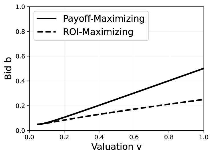
(a) $N=2$ Bidders

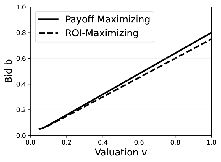
(b) $N=5$ Bidders

Figure 1: Analytical BNE for Payoff- and ROI-Maximizing Agents in a First-Price Auction with Uniform Prior

3.4 ROS-Maximizing Bidders

Finally, we analyze ROS-maximizing agents. As indicated earlier, there is an important difference between ROI and ROS: While the expected utility for ROI becomes negative once the price is higher than the value, ROS never becomes negative, independent of how high the payment is. In other words, with a monotone allocation rule, if a bidder is losing, they can always increase their bid without ever having a negative payoff. This leads to a situation where agents can place the highest possible bid, regardless of how high this value is and which payment rule is being used.

Proposition 3.1.

In the first- and second-price sealed-bid single-object auction where agents are ROS maximizers, ties are broken randomly, and the action space is bounded from above, submitting the maximal bid is an equilibrium.

Proof.

Assume all agents bid according to $\beta(v)=\bar{b}$, where $\bar{b}>0$ is the maximal bid the agents can submit. Then, the ex-interim utility is $\bar{u}(b,\beta_{-i},v_{i})=\tfrac{1}{N}\tfrac{v_{i}}{\bar{b}}>0$ if $b=\bar{b}$, and $0$ if $b<\bar{b}$. Since agents can only deviate from $\beta(v)$ by bidding less, this would strictly decrease their payoff. Therefore, $\beta(v)=\bar{b}$ is indeed an equilibrium strategy. ∎

This equilibrium strategy is also found by equilibrium learning algorithms. Obviously, this is unrealistic, because it ignores that bidders always have only a finite budget available. In this article, we consider ROS-maximizing bidders with a per-auction budget (ROSB), which we simply model using a log barrier function. This ROSB utility is given by

$$u_{i}^{ROSB}(b,v_{i})=x_{i}(b)\left(\dfrac{v_{i}}{p_{i}(b)}+\log(B-p_{i}(b))\right),$$ (13)

where $B$ is the budget. It is difficult to derive a BNE analytically for such a utility function. The first-order condition of the ex-interim utility $\bar{u}_{i}$, under the assumption of symmetric bidders, leads to

$$\dfrac{d\beta(v)}{dv} =(B-\beta(v))\dfrac{G^{\prime}(v)}{G(v)}\dfrac{v\beta(v)+\beta(v)^{2}\log(B-\beta(v))}{v(B-\beta(v))-\beta(v)^{2}}.$$ (14)

Similar to the first-order condition for ROI-maximizing bidders, this is a general non-linear ODE. But even for a uniform prior, we cannot solve this ODE analytically. As we will discuss, SODA provides a numerical technique to quickly converge to an equilibrium in all of these utility models.

4 Learning Algorithms

In the following section, we focus on the learning algorithms agents employ to increase their individual rewards. From an agent’s point of view, the repeated interaction in an auction can be interpreted as an online optimization problem. At each stage $t=1,2,\dots$ the agent chooses a strategy $x_{t}\in\operatorname{\mathcal{X}}$ from some set and gets a utility $u_{t}(x_{t})$. The utility in each stage is determined by the opponents’ current strategy, i.e., $u_{t}(\,\cdot\,)=u_{i}(\,\cdot\,,x_{-i,t})$. If we assume that $\operatorname{\mathcal{X}}$ is a closed convex subset of some vector space and $u_{t}$ are convex functions, this problem is known as an online convex optimization problem (Shalev-Shwartz 2011).

A standard performance measure of algorithms generating a sequence of strategies $x_{t}$ in such a setting is the notion of (external) regret. It is defined by

$$\text{Reg}(T)=\max_{x\in\operatorname{\mathcal{X}}}\sum_{t=1}^{T}u_{t}(x)-u_{t}(x_{t})$$ (15)

and denotes the difference between the aggregated utilities after $T$ stages and the best fixed action in hindsight. We say that an algorithm has no regret if the regret $\text{Reg}(T)$ grows sublinearly. Note that this notion of no regret does not make any assumptions on the distribution of the utilities. It is therefore especially well suited in a multi-agent setting. It is also well known that if all agents follow a no-regret algorithm in multi-agent settings such as our repeated auction, the time average of the resulting strategies converges to a coarse correlated equilibrium (CCE) (Blum and Mansour 2007). There are many no-regret learners such as follow-the-regularized-leader (FTRL), where the agent plays a regularized best response to the aggregated utility function (Shalev-Shwartz 2011). If one considers linear surrogates of the (convex) utility function, methods such as dual averaging (Nesterov 2009) can be derived from FTRL.

While FTRL requires knowledge of the functions $u_{t}$ (full information feedback) to compute an update, gradient-based methods use only the gradient $\nabla u_{t}(x_{t})$ evaluated at the $x_{t}$ to compute the linear surrogate and update the strategy (gradient feedback). Algorithms with bandit feedback require even less and rely solely on the observed utility $u_{t}(x_{t})$ of the played strategy $x_{t}$ in each stage $t$. In our experiments, we focus on algorithms in the bandit model applied to repeated auctions with finitely many actions or bids. The bandit model mimics the type of information that real-time bidding agents get in display ad auctions after bidding. SODA is an exception as it uses gradient feedback. We primarily use SODA as a numerical tool to provide us with equilibrium bidding strategies to compare against.

4.1 Exp3-Algorithm

If we consider an auction where agents have fixed valuations (complete information), the online optimization problem can be modeled as a multi-armed bandit where each arm describes one out of the possible discrete bids $b\in\operatorname{\mathcal{A}}^{d}=\{b_{1},\dots,b_{m}\}$. In general, multi-armed bandit problems are reinforcement learning problems with a single state, where a learner repeatedly chooses an action from a set of available actions and receives a reward associated with the chosen action (Lattimore and Szepesvári 2020). An agent repeatedly pulls an arm of a slot machine and aims to maximize the cumulative reward. $\varepsilon$-greedy, UCB (Upper Confidence Bound), or Exp3 (Exponential-weight algorithm for Exploration and Exploitation) are well-known no-regret bandit algorithms. We used several algorithms but will report the results of a variant of Exp3 as a representative bandit algorithm. Results for other bandit algorithms can be found in the Appendix A.1.

Input : exploration parameter $\varepsilon$, learning rate $\alpha$, number of rounds $T$

Initialize strategy $x_{1}=\tfrac{1}{m}(1,\dots,1)$;

for $t=1,2,\dots,T$ do

       Choose action $b_{t}\sim p_{t}=(1-\varepsilon)\,x_{t}+\varepsilon\,\tfrac{1}{m}\textbf{1}_{m}$;

       Receive reward $R_{t}$;

       Update strategy $x_{t+1}(b)=\dfrac{x_{t}(b)\exp(\alpha R_{t}(b)))}{\sum_{j}x_{t}(b)\exp(\alpha R_{t}(b)))}$ for all $b\in\operatorname{\mathcal{A}}^{d}$;

      

end for

Algorithm 1 Exp3-Algorithm

One key idea of Exp3 is to use an estimator for the reward of actions not played at time $t$. We focus on a specific estimator known as an importance-weighted estimator. Let $b_{t}\in\operatorname{\mathcal{A}}^{d}$ be the action played in iteration $t$ and $r_{t}\in[0,1]$ the respective reward. Then we define the importance-weighted estimator $R_{t}$ by

$$R_{t}(b)=\chi_{b_{t}}(b)\dfrac{r_{t}}{p_{t}(b_{t})},\quad\forall b\in\operatorname{\mathcal{A}}^{d}$$ (16)

where $p_{t}(b_{t})$ is the probability of playing action $b$ in stage $t$, $x_{t}\in\operatorname{\mathcal{X}}:=\Delta\operatorname{\mathcal{A}}^{d}$ the current mixed strategy, and $\chi$ the indicator function. Note that $R_{t}(b)$ is an unbiased estimate of $r_{t}$ for action $b$ conditioned on the history. This estimate is then used to update the strategy similar to the multiplicative weights update. This variant of Exp3 Braverman et al. (2017) (see Algorithm 1) has an additional exploration probability, which we can also find in the bandit version of the online stochastic mirror descent from Lattimore and Szepesvári (2020, Sec. 31). It is well-known that the Exp3 algorithm is a no-regret learner for $\varepsilon=\alpha\sim T^{-\beta}$ with $\beta\in(0,1)$ (Auer et al. 2002).

4.2 Q-Learning

Q-learning is the most well-known reinforcement learning algorithm. This is probably one reason, why it is predominantly used in the literature on algorithmic collusion (Calvano et al. 2020), and specifically by Banchio and Skrzypacz (2022). In contrast to multi-armed bandit algorithms, Q-learning can handle different states of the world in which other actions might be optimal. Note that in Banchio and Skrzypacz (2022) there is only one state and Q-learning reduces to an algorithm for a multi-armed bandit problem, a simple version of reinforcement learning.

In Algorithm 2, the input includes the discount factor $\gamma$, the learning rate $\alpha$, and the number of episodes $T$. The output is the learned Q-values for all state-action pairs. The Q-table is initialized with some initial value for all state-action pairs. The Q-learning update rule updates the Q-table based on the observed reward and the new state. The exploration-exploitation strategy used to select actions should be chosen carefully to balance exploration with exploitation. Similar to Banchio and Skrzypacz (2022), we focus on the $\varepsilon$-greedy rule, where the agent takes the action that maximizes the Q-value with probability $1-\varepsilon$ (exploitation) or takes an action at random with probability $\varepsilon$ (exploration). This allows us to compare our results to theirs. The exploration probability decays over time, e.g., according to $\varepsilon=\epsilon\exp(-\beta t)$.

Input : Discount factor $\gamma$, learning rate $\alpha$, number of rounds $T$,
exploration parameter ($\epsilon,\,\beta$), initial Q-values $Q_{0}$

Initialize Q-values $Q(b)=Q_{0}$ for all $b\in\operatorname{\mathcal{A}}^{d}$;

for $t=1,2,\dots,T$ do

       Set $\varepsilon=\epsilon\exp(-\beta t)$;

       Choose action $b_{t}\in\operatorname*{arg\,max}_{b\in\operatorname{\mathcal{A}}^{d}}Q(b)$ with probability $1-\varepsilon$ or at random with probability $\varepsilon$;

       Receive reward $r_{t}$;

       Update Q-value $Q(b_{t})=(1-\alpha)Q(b_{t})+\alpha\left[r_{t}+\gamma\max_{b}Q_{t}(b)\right]$;

      

end for

Algorithm 2 Q-Learning Algorithm without States

Note that in general, the continuation value is the maximal Q-value of the following state $s_{t+1}$, i.e., $\gamma\max_{b}Q_{t}(b,s_{t+1})$. Instead, similar to Banchio and Skrzypacz (2022), we consider a simplified version without states which reduces the Q-table to a Q-vector. Our baseline implementation is also optimistic Q-learning, where the Q-vector is initialized such that the value of Q is larger than the maximum payoff that could ever be achieved. The purpose of such an initialization is to ensure that the algorithm won’t stop experimenting until all of the Q-values have sufficiently decreased. Banchio and Skrzypacz (2022) argue that in their multi-agent setting, the advantage offered by optimism is a phase of experimentation at the beginning, which improves convergence. We find that the initialization is crucial and also explore alternative initializations in our experiments.

4.3 Extensions to Model Incomplete Information

The algorithms described so far were based on the model of complete-information game where the values of the bidders are publicly known. In practice, bidders do not have complete information and algorithms need to take into account incomplete information. This can be done by discretizing the type or valuation space $\operatorname{\mathcal{V}}^{d}:=\{v_{1},\dots,v_{n}\}\subset\operatorname{\mathcal{V}}$ of bidders with a corresponding prior distribution $F^{d}$. The discrete spaces can be constructed from the continuous game $\operatorname{\mathcal{G}}$ using a subset of equidistant points from the spaces and a numerical integration rule to derive a discretized prior $F^{d}$. Overall, this defines a discrete incomplete-information game $\operatorname{\mathcal{G}}^{d}=(\operatorname{\mathcal{I}},\operatorname{\mathcal{V}}^{d},\operatorname{\mathcal{A}}^{d},u,F^{d})$ for the standard continuous Bayesian game as it is described in textbooks (Krishna 2009).

The standard bandit algorithms are not defined for games with incomplete information. However, an interpretation as a population game (Hartline et al. 2015) allows for an extension that can be readily implemented. For this, we consider $N$ populations, where each population $i\in\operatorname{\mathcal{I}}$ consists of $n=|\operatorname{\mathcal{V}}^{d}|$ players. All players within a population have different types $v\in\operatorname{\mathcal{V}}^{d}$. We write $v_{i}$ the player from population $i$ with valuation $v\in\operatorname{\mathcal{V}}^{d}$. In the population game, nature draws a player from each population according to the prior $F^{d}$, i.e., $v_{i}\sim F^{d}$ for all populations $i\in\operatorname{\mathcal{I}}$, who play against each other. Since this game is a complete-information game with finite actions, we can directly apply the algorithms described previously and learn a strategy for each $v_{i}$ of some population $i$. Aggregating the strategies over all $v_{i}$ gives us a strategy for agent $i$ in the discrete incomplete-information game.

4.4 SODA

Let us also describe a gradient-based method, the SODA learning algorithm (Bichler et al. 2023). This method provides us with an equilibrium strategy to compare against in situations where no analytical solution is available.

The SODA learning algorithm also acts on the discretized auction game $G^{d}$. The main idea is to use distributional strategies in the discretized auction game. Distributional strategies are an extension of mixed strategies in complete-information games to settings with incomplete information (Milgrom and Weber 1985). They can be represented by matrices $s\in\operatorname{\mathbb{R}}^{n\times m}$, where each entry $s_{ij}$ of this matrix represents the probability of a valuation-action pair $(v_{i},b_{j})\in\operatorname{\mathcal{V}}^{d}\times\operatorname{\mathcal{A}}^{d}$. To be consistent with the auction game the distributional strategy has to satisfy the marginal condition $\sum_{j=1}^{m}s_{ij}=F^{d}(v_{i})$, i.e., the probability of a value over all actions has to be equal to the probability of the value given by the prior. We denote the set of such distributional strategies by $\operatorname{\mathcal{S}}$. Given a profile of such discrete distributional strategies, one can compute the expected utility $\tilde{u}_{i}$ as sum over all outcomes weighted by the probabilities induced by $s=(s_{1},\dots,s_{N})$. If we consider an example with $N=2$ agents, we get an expected utility for agent 1 by

$$\tilde{u}_{1}(s_{1},s_{2})=\sum_{i_{1},j_{1}=1}^{n,m}(s_{1})_{i_{1}j_{1}}\sum_{i_{2},j_{2}=1}^{n,m}(s_{2})_{i_{2}j_{2}}\,u_{1}(b_{j_{1}},b_{j_{2}},v_{i_{1}}),$$ (17)

where $u_{1}(b_{1},b_{2},v)$ is the ex-post utility.

The expected utility together with the set of distributional strategies allows us to interpret the auction game as a complete-information game $\Gamma=(\operatorname{\mathcal{I}},\operatorname{\mathcal{S}},\tilde{u})$. Note that the set of discrete distributional strategies is a compact and convex subset of $\operatorname{\mathbb{R}}^{n\times m}$ and the expected utility is differentiable and linear in the bidder’s own strategy. This allows us to rely on standard tools from online convex optimization to compute the NE of $\Gamma$, which corresponds to a BNE of $\operatorname{\mathcal{G}}^{d}$.

In our experiments, we use dual averaging (Nesterov 2009) with an entropic regularization term (known as exponentiated gradient ascent) and mirror ascent (Nemirovskij and Yudin 1983) with an Euclidean mirror map (standard projected gradient ascent).

Input: Initial distributional strategy $s_{1}$, sequence of step sizes $\{\eta_{t}\}_{t=1}^{T}$

Initialize $y_{i,t}=0$ for all $i\in\operatorname{\mathcal{I}}$ for $t=1,2,\dots,T$ do

      for each agent $i\in\mathcal{I}$ do

           observe gradient $c_{i,t}=\nabla_{s_{i}}\tilde{u}_{i}(s_{i,t},s_{-i,t})$;

           update dual variable $y_{i,t+1}=y_{i,t}+\eta_{t}c_{i,t}$;

           update strategy $s_{i,t+1}=\operatorname*{arg\,min}_{s\in\operatorname{\mathcal{S}}^{d}}\|s-y_{i,t+1}\|_{2}^{2}$;

          

           end for

          

           end for

Algorithm 3 Simultaneous Online Dual Averaging (SODA)

Given the respective method, all agents simultaneously compute their individual gradients and perform the corresponding update step, as described in Algorithm 3 for dual averaging. Specifically for dual averaging, one can show that if this procedure converges to a single point $s\in\operatorname{\mathcal{S}}^{d}$, then this strategy profile is a NE in the approximation game, and thereby a BNE for the discretized auction game (Bichler et al. 2023, Corollary 1). Moreover, for some single-object auction formats, such as first- or second-price sealed-bid and all-pay auctions, it is shown that if SODA finds an approximate equilibrium of the discretized auction game, this is also an approximate equilibrium of the continuous game (Bichler et al. 2023, Theorem 1). Therefore, SODA provides an ex-post certificate.

Note that SODA serves only as a baseline as it allows us to approximate the BNE quickly and with high accuracy. It is not meant as an algorithm to simulate display ad auctions. While bandit algorithms such as Exp3 only require information about the price and whether they won or lost in an auction, in SODA the auctioneer would need all agents’ mixed strategies to provide the respective feedback for the agents.

5 Results

In this section we report the results of learning dynamics under different learning algorithms, different informational assumptions, and different utility models, to analyze revenue in repeated first-price auctions compared to their second-price counterparts.

5.1 Experimental Design

In our experiments we simulate $N\in\{2,3\}$ independent agents bidding in repeated first- and second-price auctions. Each experiment consists of $T$ iterations and is repeated $10$ times. We focus on experiments with bandit feedback, where in each iteration $t\in\{1,\dots,T\}$, agents submit their bid from some discrete action space $b_{t}\in\operatorname{\mathcal{A}}^{d}\subset\operatorname{\mathcal{A}}=[0,1]$, observe their utility (bandit feedback), and update their bidding strategies according to some learning algorithm. The objective of the agents is to maximize their utility, which depends on the bids of all agents and on their own valuation $v_{t}\in\operatorname{\mathcal{V}}^{d}\subset\operatorname{\mathcal{V}}=[0,1]$ from some discrete type space.

We will first discuss the complete-information model where the agents have a fixed valuation $v_{t}=1$. We are interested in comparing the performance of different learning algorithms in the first- and second-price auction with payoff-maximizing agents, i.e., quasi-linear utility functions. We run each experiment for $T=5\cdot 10^{5}$ iterations.

In the incomplete-information model, the valuations of each agent are drawn uniformly (i.i.d.) in each iteration, i.e., $v_{t}\sim U(\operatorname{\mathcal{V}}^{d})$. Using the population game interpretation described in Section 4.3, we learn a separate strategy for each of the agent’s valuations, which allows us to use the algorithms from the complete-information setting. Since each agent-value pair gets less feedback that way, we run these experiments for $T=10^{7}$ iterations. The experiments differ not only in the payment rule but also in the utility function of the agents, namely quasi-linear (QL), ROI, and ROSB. For ROI and ROSB to be well defined, we introduce a reserve price $r=0.05$, which we also use in the QL setting for better comparison. The budget parameter for ROSB maximizing agents is equal to $B=1.01$ in what we report. In addition to the bandit algorithms, we use SODA to get a good approximation of the equilibrium strategies in the incomplete-information models and to serve as a baseline for the algorithms with bandit feedback.

5.2 Complete-Information Models

Setting

Two agents $i\in\{1,2\}$ bid in a first- and second-price auction. All agents value the item at $v=1$ and choose bids from $\operatorname{\mathcal{A}}^{d}=\{0.05,0.10,\dots,0.90,0.95\}$. For the first-price auction, it can be shown that with two agents and a random tie-breaking rule, the NE is to bid $b_{1}=b_{2}=0.95$ or $b_{1}=b_{2}=0.90$ for both of them. With more than 2 bidders, the NE is to only bid $b_{i}=0.95$ for all $i\in\{1,\dots,N\}$. In the second-price auction, the unique NE is $b_{1}=b_{2}=0.95$.

Results

Below, we report on experiments with Exp3 and Q-learning with the parameters as defined in Table 1. The main results are summarized in Figure 2.

Table 1: Parameters for Bandit Algorithms

Learner	Init.	$\epsilon$	$\beta$	$\gamma$	$\alpha$	$Q_{0}$
Optimistic (Baseline)	100	0.025	0.0002	0.99	0.05	100
Optimistic & small $\gamma$	100	0.025	0.0002	0.25	0.05	100
Optimistic & fix $\varepsilon$	100	0.025	0.0	0.99	0.05	100
Zero	0	0.025	0.0	0.99	0.05	0
Exp3	uniform	0.01	0.0	-	0.01	-

Optimistic (Baseline) corresponds to the parameters from Banchio and Skrzypacz (2022).

Result 1.

The collusive outcomes by using Q-Learning in the complete-information setting from Banchio and Skrzypacz (2022) relies on the parameters of the Q-values. We find evidence that optimistic initialization enables collusive outcomes while lower initializations or lower discount rates lead to higher prices closer to the equilibrium.

First, we consider two symmetric agents using variations of the Q-learner considered by Banchio and Skrzypacz (2022), which serves as a baseline. Banchio and Skrzypacz (2022) used an optimistic initialization for their learners, which we replicate by setting the initial Q-values to $\tfrac{1}{1-\gamma}$. We can reproduce their results but observe that parameter changes lead to higher prices compared to this baseline Q-learner (see Figure 2).

Without the decreasing exploration rate (fix $\varepsilon$), we see cyclic behavior where the q-learner often returns to low prices but fails to converge to a fixed policy. Even more interesting is the observation that initializing the Q-values with zero (and fixed exploration rate) instead of optimistic leads to a completely different outcome where the learner converges to the Nash equilibrium. One possible explanation is that collusive prices are more stable for higher Q-values since the rewards are much higher. This way, the learning algorithm might get stuck with lower bids. If we remove this hidden preference for low actions by initializing differently, higher actions are played. It is also interesting to note that if we stick to optimistic initialization but have a small discount factor $\gamma$, the learners also converge to higher prices closer to the equilibrium.

(a) Q-Learner vs. Q-Learner (Symmetric Agents)

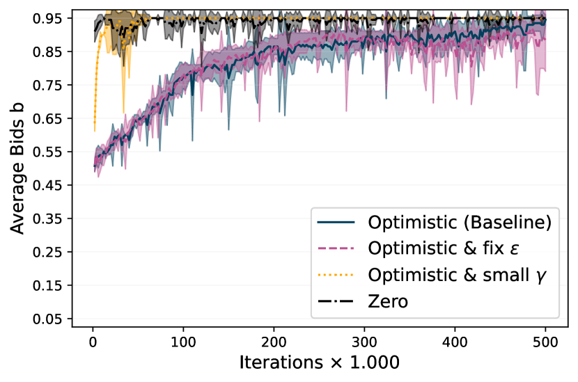
(b) Q-Learner vs. Exp3 (Asymmetric Agents)

Figure 2: Median Bids for 2 Agents in the FPSB Auction Using Different Q-Learners and Exp3

We split the learning process into intervals of two thousand iterations and compute the median bid of an agent for each interval. The shaded area shows the mean $\pm$ std of these median bids over 10 runs, i.e., repetitions of the experiment, for one agent. In the first plot, we show experiments for different parameters of the Q-learner used by both agents (symmetric). In the second plot, we show the results for agents using different learning algorithms (asymmetric), i.e., Q-learner with different parameters and Exp3, to play against an agent using the Exp3 learning algorithm. Note that we report the median instead of the average bid since the exploration makes the average bid harder to interpret, especially when we converge to high bids.

Result 2.

If we use an Exp3 and a Q-learning algorithms, Q-learning becomes more robust and agents bid significantly higher compared to the symmetric case with identical Q-learners.

The second plot in Figure 2 shows additional experiments where the second agent uses the Exp3 algorithm, which we use as an example for no-regret bandit algorithms. If both agents use Exp3, they converge to a Nash equilibrium quickly. If Q-learners compete against Exp3, we observe significantly higher bids compared to the symmetric settings in the first plot. In most cases, the Q-learner even converges to a Nash equilibrium, even though it takes more iterations.

5.3 Incomplete-Information Model

In the following experiments we make the arguably more realistic assumption that valuations of opponents are only known in distribution and study this Bayesian setting under different utility models.

5.3.1 Equilibria Learned with SODA

Before we analyze bandit algorithms in this setting, we use SODA on a finer discretization to get a good approximation of the equilibrium strategies since analytical solutions are not available for all settings (see discussion in Section 3).

Setting

The action and type space $\operatorname{\mathcal{A}}=\operatorname{\mathcal{V}}=[0,1]$ of the $N=2$ agents are discretized using $n=m=64$ equidistant points. We consider the first- and second-price auction under different utility models, namely QL, ROI, and ROSB maximizing agents.

Results

To measure the quality of computed strategies, we use the relative utility loss $\ell$ as a metric. Given a distributional strategy $s_{i}$, $\ell$ measures the relative improvement of the expected utility we can get by best responding to the other agents strategies $s_{-i}$, i.e.,

$$\ell(s_{i},s_{-i})=1-\dfrac{\tilde{u}_{i}(s_{i}^{br},s_{-i})}{\tilde{u}_{i}(s_{i},s_{-i})}.$$ (18)

Note that in the discretized game, the best response $s_{i}^{br}$ is the solution of a simple LP. If the absolute utility loss $\ell\cdot\tilde{u}_{i}(s_{i},s_{-i})<\varepsilon$ for all agents, the computed strategy profile is a $\varepsilon$-BNE in the discretized auction game. In our experiments we observe that on average $\ell\leq 10^{-3}$ in all instances. Moreover, we observe that we closely approximate the known equilibrium strategies for QL and ROI. More details on these experiments and additional results for $N=3$ agents can be found in the Appendix A.2.1.

(a) [First-Price

(b) [Second-Price

(c) Expected Revenue

Figure 3: Results for SODA with 2 Bidders with Uniform Prior

The first two plots show the mean and standard deviation of 100 sampled bids from the computed strategies for each discrete valuation in settings with $n=2$ bidders, uniform prior, and different utility functions for the first- and second-price auction. The black line shows the analytical BNE (only known for QL and ROI). In the third plot we use the computed strategies to approximate the expected revenue by simulating $2^{22}$ auctions for each setting.

We use the computed equilibrium strategies to simulate auctions to approximate the expected revenue. An important insight from this analysis (see Figure 3) is that revenue equivalence breaks for return-on-invest and return-on-spend (with budget) maximizing agents and that revenue in first-price auctions is lower compared to the second-price auctions in equilibrium.

5.3.2 Bandit Algorithms

Real-world bidding agents only get bandit feedback, and the question is now whether the revenue in the first-price auction is also lower when we employ bandit algorithms (e.g., Exp3) in the ROI and the ROSB utility models. Since learning is much slower for learners with bandit feedback compared to SODA, we use a coarser discretization similar to the complete information setting.

Setting

We discretize the type and action space with $\operatorname{\mathcal{V}}^{d}=\operatorname{\mathcal{A}}^{d}=\{0,0.05,\dots,0.95,1\}$ which corresponds to $n=m=21$ discretization points. We focus on repeated first- and second-price auctions with $N=3$ agents and different assumptions on the utility function. As described in Section 4.3, each agent is represented by a population, which consists of different valuations. This means each agent (i.e. population) has $n=21$ different instances of the bandit learner, i.e., one for each valuation. To get comparable results to the complete information, we increase the number of iterations approximately by the number of discrete values, which leads to $10^{7}$ iterations instead of $5\cdot 10^{5}$. In our experiments we use Exp3 with a fix exploration rate $\varepsilon=0.01$ and learning rate $\alpha=0.01$. For ROI and ROSB we use a smaller learning rage $\alpha=0.0005$ since the magnitude of the utilities is larger.

Results

First, we observe that the revenues generated by the agents using Exp3 show a similar pattern to the expected revenues in equilibrium (see previous subsection). We see that revenue equivalence does not hold for ROI and ROSB maximizing agents and especially for ROI maximizing agents, the revenue for the first-price auction is significantly lower compared to the second-price auction. Furthermore, the average revenue matches the values predicted by the Bayes-Nash equilibrium strategies in the discretized setting. These are approximated using SODA, where the strategies are updated using mirror ascent with a decreasing stepsize $\eta=0.025\cdot t^{-0.05}$. The computed strategies have a relative utility loss $\ell<0.1\%$.

(a) Payoff-Maximizing

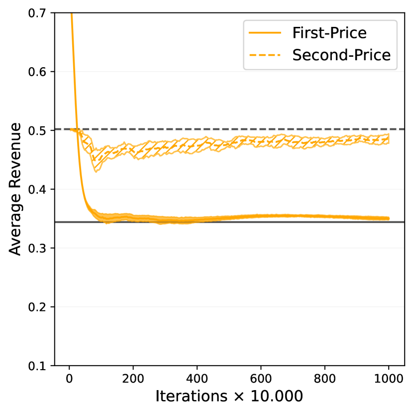
(b) ROI-Maximizing

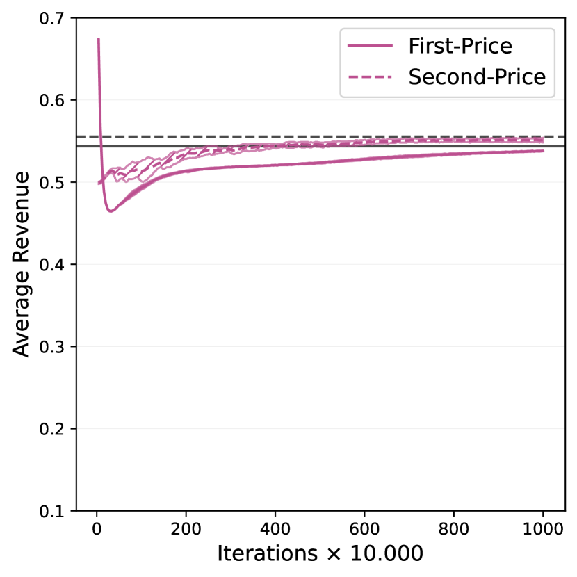
(c) ROSB-Maximizing

Figure 4: Revenue for Exp3 with 3 Bidders with Uniform Prior

We run Exp3 for $10$ million iterations and compute the average revenue for all $20\thinspace 000$ iteration intervals for payoff, ROI and ROSB maximizing agents. We plot the mean and standard deviations of this average revenue per interval over 10 runs. The black horizontal lines denote the expected revenue we would get with the BNE strategies computed using SODA.

Not only is the average revenue close to the predictions from the equilibrium analysis, but we can also observe that the agents actually learn to play according to the Bayes-Nash equilibrium using a bandit algorithm such as Exp3. To this end, we look at the frequency of the bids within an interval and compare it to the distributional equilibrium strategy computed using SODA.

Result 3.

If we use Exp3 in the incomplete-information auction setting, the agents learn to bid according to the BNE and revenues for the first-price auction are lower compared to the second-price auctions for ROI and ROSB maximizing agents, as predicted by the equilibrium analysis.

As we can see in Figure 5 - 6, the empirical frequency of actions played by Exp3 converges to the equilibrium strategies. Similar plots for ROSB-maximizing agents and the second-price counterparts and a Gaussian prior can be found in the Appendix A.2.2.

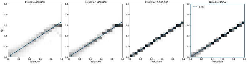
Figure 5: Strategies for Payoff-Maximizing Agents using Exp3 in the FPSB Auction with Uniform Prior

We run Exp3 for $10$ million iterations and visualize the frequency of the last $20\thinspace 000$ bids w.r.t. the values after $0.4$, $1$, and $10$ million iterations. On the last plot, we show the distributional equilibrium strategy computed by SODA. The colored lines denote the BNE in the continuous setting.

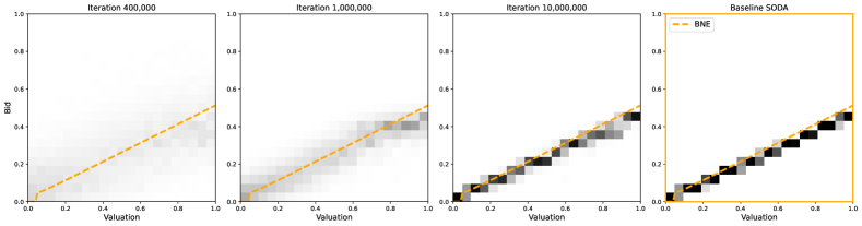
Figure 6: Strategies for ROI-Maximizing Agents using Exp3 in the FPSB Auction with Uniform Prior

We run Exp3 for $10$ million iterations and visualize the frequency of the last $20\thinspace 000$ bids w.r.t. the values after $0.4$, $1$, and $10$ million iterations. On the last plot, we show the distributional equilibrium strategy computed by SODA. The colored lines denote the BNE in the continuous setting.

6 Conclusions

In this paper, we study the impact that a move from second-price to first-price auctions can have on the revenue of an ad exchange that faces learning agents. Recent research provided evidence that Q-learning in repeated auctions in a complete-information model with payoff-maximizing agents can lead to tacit collusion and lower revenue in the first-price auction (Banchio and Skrzypacz 2022). Our experiments show that with different hyper-parameters, Q-learning does converge to the Nash equilibrium in this model. Importantly, when bidders use other bandit algorithms, we do not find evidence for algorithmic collusion and revenue equivalence holds in this model. Recent theoretical results confirm that a wide range of mean-based learning algorithms converge to equilibrium. While Banchio and Skrzypacz (2022) show that algorithmic collusion can occur with complete information, these results suggest that the phenomenon might be limited to specific algorithms and parameter settings.

In real-world display ad auctions, bidders neither have complete information nor do they necessarily maximize payoff. ROI or ROSB maximization is widely described in the literature. First, we show that gradient-based learners and bandit learners converge to an equilibrium in all three utility models. This suggests that tacit collusion is also less of a concern in the standard incomplete-information model. However, revenue equivalence breaks in auctions with ROI- or ROSB-maximizing bidders, and the revenue of the first-price auction is lower in such models.

As in prior research about algorithmic collusion, we analyze models of repeated identical auctions, where agents maximize their separable utility for individual auctions. In the field, the types of impressions on auctions vary over time and so does the competition. Also, the algorithms used by bidders in display ad auctions are likely to differ across bidding firms. What we can say is that the phenomenon of algorithmic collusion does not arise with a variety of bandit learning algorithms that have been cited in the literature and that provide natural candidates. This makes algorithmic collusion less likely to appear in real-world environments as well. Interestingly, we find that for the very different utility models and incomplete information, bandit as well as gradient-based algorithms converge to an equilibrium. The reasons for such consistent convergence in incomplete-information models are of independent interest but outside the scope of this paper (see Bichler et al. (2023) for a related discussion).

Appendix A Additional Experiments

A.1 Complete-Information Model

Since we only considered Exp3 as a better alternative to Q-learning, we want to run similar experiments for other bandit algorithms as well, to check if the results are robust with respect to different learning algorithms. We consider three well-known bandit learners that handle the exploration-exploitation tradeoff differently (see for instance Sutton and Barto (2018), Lattimore and Szepesvári (2020)).

$\varepsilon$-Greedy. This policy compares the current average reward of each action $a$, which is defined by

$$\hat{R}(a)=\dfrac{\sum_{s=1}^{t}\chi_{a}(a_{t})r_{s}(a_{t})}{N(a_{t})}$$ (19)

with $\chi_{a}(a_{t})=1$ if $a_{t}=a$ and $0$ else. $N_{t}(a)$ denotes the number an action $a$ has been played up to iteration $t$. The $\varepsilon$-Greedy selects the action with the highest average reward with probability $1-\varepsilon_{t}$ and some random action with probability $\varepsilon_{t}$ ( $\varepsilon_{t}=0.05$ in our experiments).

UCB1. Instead of exploring actions at random, UCB1 explores only actions with enough potential or uncertainty (upper-confidence-bound action selection). This is achieved by taking the action with the maximal value which consists of the average reward and an exploration bonus depending on the number an action as been visited. This value is given by

$$\hat{R}(a)+c\sqrt{\dfrac{\ln t}{N_{t}(a)}},$$ (20)

where $c$ is some exploration parameter ($c=4$ in our experiments).

Thompson-Sampling. Finally, we also use a Bayesian method first introduced in (Thompson 1933). Thompson sampling assumes a distribution $\operatorname{\mathcal{P}}_{r}(\theta_{a})$ (with some parameter $\theta_{a}$) over the rewards of each action. In each iteration $t$, the learner sample parameters $\theta_{a}^{t}\sim\operatorname{\mathcal{P}}_{\theta}$ from some parameter distribution for each action $a$, play the action $a^{*}$ that maximizes the expected reward given the distribution $\operatorname{\mathcal{P}}_{r}(\theta_{a}^{t})$, and update the parameter distribution $\operatorname{\mathcal{P}}_{\theta}$ for action $a^{*}$ given the observed reward $r_{t}(a^{*})$. In our implementation, we assume that the rewards for each action follow a Gaussian distribution (with known variance $\sigma$) and thereby use a Gaussian prior for the parameter $\theta_{a}=\mu_{a}$ (conjugate prior).

Repeating the experiments with two players in a complete-information first-price sealed bid (Section 5.2) for different bandit algorithms, we observe that most of them converge to the Nash equilibrium (Figure 7).

(a) Bandit vs. Bandit (Symmetric Agents)

(b) Bandit vs. Exp3 (Asymmetric Agents)

Figure 7: Median Bids for 2 Agents in the FPSB Auction Using Different Bandit Algorithms

We split the learning process into intervals of two thousand iterations and compute the median bid of an agent for each interval. The shaded area shows the mean $\pm$ std of these median bids over 10 runs, i.e., repetitions of the experiment, for one agent. In the first plot, we show experiments for different bandit algorithms used by both agents (symmetric). We report the median instead of the average bid since the exploration makes the average bid harder to interpret, especially when we converge to high bids. In the second plot, we show the results for agents using different learning algorithms (asymmetric), i.e., bandit learning algorithms against an agent using the Exp3.

The exception here is UCB1, which shows similar behavior to the Q-learner from Banchio and Skrzypacz (2022). But again, when playing against another bandit algorithm, such as Exp3, the bids are significantly higher.

If we compare the revenue under different payment rules for the Q-learner and different bandit algorithms (assuming symmetric agents), we can confirm the observations by Banchio and Skrzypacz (2022) that the revenue in the first-price auction is significantly lower than in the second-price auction for their Q-Learner with optimistic initialization. But, our experiments further indicate that this might be specific to this learning algorithm. Overall, we observe that the first-price auctions might be harder to learn for some algorithms (i.e., some instances of Q-learning and UCB1). And since a failure to learn the Nash equilibrium automatically leads to lower revenue, these methods might seem to collude. But in fact, other versions of Q-learning (i.e., with zero initialization) show opposite results, and a number of reasonable bandit algorithms converge in both settings. Note that the slightly lower revenue (see Figure 8) in the first-price auction compared to the second-price auction for $\varepsilon$-Greedy, Thompson-Sampling, and Exp3 can be explained by the additional Nash equilibrium at $0.90$ for the first-price auction.

(a) Q-Learner

(b) Bandit Algorithms

Figure 8: Revenue of the First- and Second-Price Auction with 2 agents

We compute the average revenue over the last $100\thinspace 000$ iterations (excluding the initial learning phase) and report the mean and standard deviation over 10 runs of the experiment.

A.2 Incomplete-Information Model

A.2.1 SODA

We applied SODA to the first- and second-price auctions with different utility models and quickly converge to a pure-strategy BNE. As described in Section 4.4, SODA acts on a discretized version we construct by discretizing the valuation and action space using $n=m=64$ equidistant points. Due to better performance, we use a tie-breaking rule in which both agents lose in ties for this discretization. The strategies are updated in each iteration using dual averaging with the entropic regularization term and a decreasing step size $\eta_{t}=10\cdot t^{-0.05}$. We stop the learning algorithm after $5\thinspace 000$ iterations, or whenever the relative utility loss $\ell$ of all agents in the discretized game is less than $10^{-4}$. Each experiment is repeated $10$ times. To verify the computed strategies, we compare them to the analytical solutions in the settings where the BNE is known. To this end, we report the following metrics (similar to Bichler et al. (2021, 2023)):

Relative Utility Loss $\operatorname{\mathcal{L}}$. We approximate the expected utility using the sample-mean of the ex-post utilities, i.e., $\tilde{u}_{i}(\beta_{i},\beta^{*}_{-i})\approx\hat{u}_{i}(\beta_{i},\beta^{*}_{-i}):=\tfrac{1}{n_{v}}\sum_{v}u_{i}(\beta_{i}(v_{i}),\beta_{-i}((v_{-i})))$. The relative loss in the expected utility the agent receives when playing the computed strategy $s_{i}$ instead of the analytical equilibrium $\beta_{i}^{*}$

$$\mathcal{L}_{i}(\beta_{i})\ =\ 1-\frac{\hat{u}_{i}(\beta_{i},\beta^{*}_{-i})}{\hat{u}_{i}(\beta^{*}_{i},\beta^{*}_{-i})},$$ (21)

while all other agents play the equilibrium strategy $\beta^{*}_{-i}$.

$L_{2}$ Distance. The probability-weighted root mean squared error of $\beta_{i}$ and $\beta^{*}_{i}$ in the action space, which approximates the $L_{2}$ distance of these two functions:

$$L_{2}(\beta_{i})\ =\ \bigg{(}\frac{1}{n_{\text{batch}}}\sum_{v_{i}}\left(\beta_{i}(v_{i})-\beta^{*}_{i}(v_{i})\right)^{2}\bigg{)}^{\frac{1}{2}}.$$ (22)

This way we ensure that our computed strategy not only performs similarly in terms of utility, but also approximates the actual known BNE.

To compute these metrics, we sample valuations (batch size $n_{v}=2^{22}$), identify for each valuation the nearest discrete valuation $v\in\operatorname{\mathcal{V}}^{d}$, and then sample a discrete bid $b\in\operatorname{\mathcal{A}}^{d}$ from the computed strategy. The sampled bids are denoted by $\beta_{i}(v)$ in the definitions above. The same simulation procedure is used to approximate the expected revenue from Figure 3.

Table 2: Results for SODA

Bidders	Utility Model	Pricing Rule	$\ell$	$\mathcal{L}$	$L_{2}$
$n=2$	Quasi-Linear (QL)	First-Price	0.000 (0.000)	0.002 (0.000)	0.010 (0.001)
		Second-Price	0.000 (0.000)	0.001 (0.000)	0.013 (0.000)
	Return-on-Invest (ROI)	First-Price	0.000 (0.000)	0.014 (0.001)	0.013 (0.000)
		Second-Price	0.000 (0.000)	0.000 (0.000)	0.016 (0.000)
$n=3$	Quasi-Linear (QL)	First-Price	0.000 (0.000)	0.001 (0.000)	0.010 (0.001)
		Second-Price	0.000 (0.000)	0.001 (0.000)	0.014 (0.000)
	Return-on-Invest (ROI)	First-Price	0.000 (0.000)	0.004 (0.000)	0.011 (0.000)
		Second-Price	0.000 (0.000)	0.001 (0.000)	0.013 (0.000)

The mean (and standard deviation) of the relative utility loss in the discretized game $\ell$ and the approximated utility loss $\mathcal{L}$ and the $L_{2}$ norm w.r.t. the analytical BNE are reported for different number of agents $n\in\{2,3\}$ and different utility models, i.e., payoff-maximizing bidders and ROI-maximizing. In all settings, we assume a uniform prior.

As Table 2 shows, the computed strategies of the discretized game closely approximate the analytical BNE in the original continuous setting. We repeat the experiments for a truncated Gaussian prior ($\mu=0.5,\,\sigma=0.15$) over the interval $[0,1]$. Again we observe convergence in the discretized game with an average relative utility loss $\ell\leq 0.001$ over 10 runs in all settings. The results are similar to the uniform case. Again, revenue for the first-price auction is lower compared to the second-price auction.

(a) First-Price

(b) Second-Price

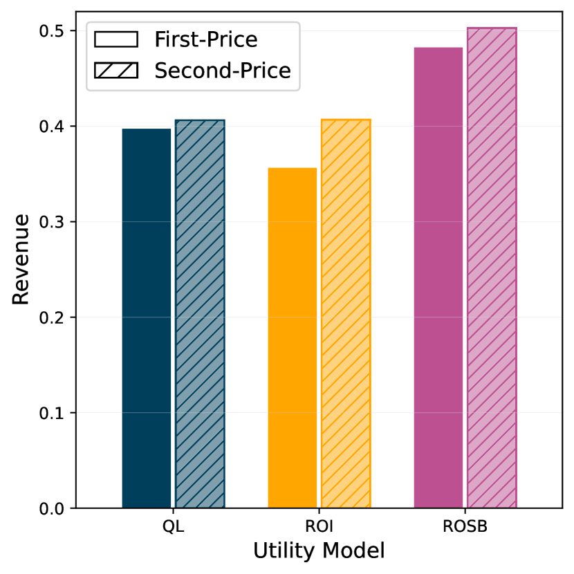
(c) Expected Revenue

Figure 9: Results for SODA with 2 Bidders with (truncated) Gaussian Prior

The first two plots show the mean and standard deviation of 100 sampled bids from the computed strategies for each discrete valuation in settings with $n=2$ bidders, uniform prior, and different utility functions for the first- and second-price auction. The black line shows the analytical BNE (only known for QL and ROI). In the third plot we use the computed strategies to approximate the expected revenue by simulating $2^{22}$ auctions for each setting.

A.2.2 Exp3

The learning progress of Exp3 in the remaining settings not shown in Section 5.3.2, i.e., first-price auction of ROSB maximizing agents andsecond-price auction for payoff, ROI, and ROSB maximizing agents are shown in the following figures. The plots show the frequency of the last $20\thinspace 000$ bids w.r.t. the different values after $0.4$, $1$, and $10$ million iterations. In the last plot of each figure, we show the distributional equilibrium strategy computed by SODA. The colored lines denote the analytical BNE in the continuous setting. The key observation is that Exp3, which only uses bandit-feedback is able to learn the BNE in the considered settings.

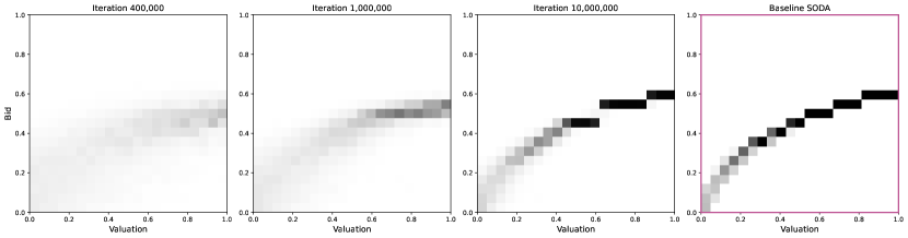
Figure 10: Strategies for ROSB-Maximizing Agents using Exp3 in the FPSB Auction with Uniform Prior

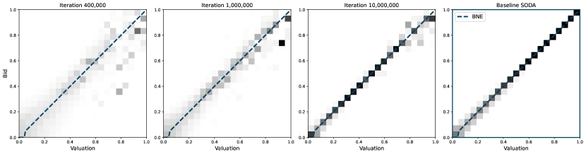
Figure 11: Strategies for Payoff-Maximizing Agents using Exp3 in the SPSB Auction with Uniform Prior

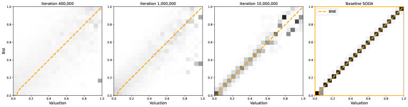
Figure 12: Strategies for ROI-Maximizing Agents using Exp3 in the SPSB Auction with Uniform Prior

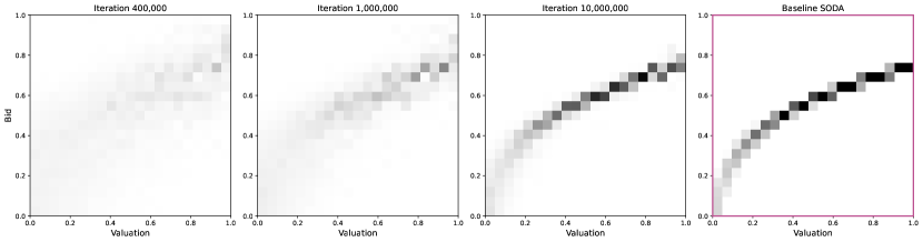
Figure 13: Strategies for ROSB-Maximizing Agents using Exp3 in the SPSB Auction with Uniform Prior

References

- Alcobendas and Zeithammer (2021) Alcobendas M, Zeithammer R (2021) Adjustment of bidding strategies after a switch to first-price rules. Available at SSRN 4036006 .
- Armantier et al. (2008) Armantier O, Florens JP, Richard JF (2008) Approximation of Nash equilibria in Bayesian games. Journal of Applied Econometrics 23(7):965–981, ISSN 08837252, 10991255, URL http://dx.doi.org/10.1002/jae.1040.
- Asker et al. (2022) Asker J, Fershtman C, Pakes A (2022) Artificial Intelligence, Algorithm Design, and Pricing. AEA Papers and Proceedings 112:452–456, URL http://dx.doi.org/10.1257/pandp.20221059.
- Assad et al. (2020) Assad S, Clark R, Ershov D, Xu L (2020) Algorithmic Pricing and Competition: Empirical Evidence from the German Retail Gasoline Market. URL http://dx.doi.org/10.2139/ssrn.3682021.
- Auer et al. (2002) Auer P, Cesa-Bianchi N, Freund Y, Schapire RE (2002) The nonstochastic multiarmed bandit problem. SIAM Journal on Computing 32(1):48–77, URL http://dx.doi.org/10.1137/S0097539701398375.
- Ausubel and Baranov (2020) Ausubel LM, Baranov O (2020) Core-selecting auctions with incomplete information. International Journal of Game Theory 49:251–273, ISSN 1432-1270, URL http://dx.doi.org/10.1007/s00182-019-00691-3.
- Bailey and Piliouras (2018) Bailey JP, Piliouras G (2018) Multiplicative weights update in zero-sum games. Proceedings of the 2018 ACM Conference on Economics and Computation, 321–338 (ACM).
- Balduzzi et al. (2018) Balduzzi D, Racaniere S, Martens J, Foerster J, Tuyls K, Graepel T (2018) The mechanics of n-player differentiable games. Dy J, Krause A, eds., Proceedings of the 35th International Conference on Machine Learning, volume 80 of Proceedings of Machine Learning Research, 354–363 (PMLR), URL https://proceedings.mlr.press/v80/balduzzi18a.html.
- Balseiro and Gur (2019) Balseiro SR, Gur Y (2019) Learning in repeated auctions with budgets: Regret minimization and equilibrium. Management Science 65(9):3952–3968.