Deep Equilibrium Based Neural Operators for Steady-State PDEs
Abstract
Data-driven machine learning approaches are being increasingly used to solve partial differential equations (PDEs). They have shown particularly striking successes when training an operator, which takes as input a PDE in some family, and outputs its solution. However, the architectural design space, especially given structural knowledge of the PDE family of interest, is still poorly understood. We seek to remedy this gap by studying the benefits of weight-tied neural network architectures for steady-state PDEs. To achieve this, we first demonstrate that the solution of most steady-state PDEs can be expressed as a fixed point of a non-linear operator. Motivated by this observation, we propose FNO-DEQ, a deep equilibrium variant of the FNO architecture that directly solves for the solution of a steady-state PDE as the infinite-depth fixed point of an implicit operator layer using a black-box root solver and differentiates analytically through this fixed point resulting in training memory. Our experiments indicate that FNO-DEQ-based architectures outperform FNO-based baselines with the number of parameters in predicting the solution to steady-state PDEs such as Darcy Flow and steady-state incompressible Navier-Stokes. Finally, we show FNO-DEQ is more robust when trained with datasets with more noisy observations than the FNO-based baselines, demonstrating the benefits of using appropriate inductive biases in architectural design for different neural network based PDE solvers. Further, we show a universal approximation result that demonstrates that FNO-DEQ can approximate the solution to any steady-state PDE that can be written as a fixed point equation.
1 Introduction
Partial differential equations (PDEs) are used to model a wide range of processes in science and engineering. They define a relationship of (unknown) function and its partial derivatives. Most PDEs do not admit a closed form solution, and are solved using a variety of classical numerical methods such as finite element (LeVeque, 2007), finite volume (Moukalled et al., 2016), and spectral methods (Kopriva, 2009; Boyd, 2001). These methods are often very computationally expensive, both as the ambient dimension grows, and as the desired accuracy increases.
This has motivated a rapidly growing area of research in data-driven approaches to PDE solving. One promising approach involves learning neural solution operators (Chen and Chen, 1995; Lu et al., 2019; Bhattacharya et al., 2021; Li et al., 2020b), which take in the coefficients of a PDE in some family and output its solution—and are trained by examples of coefficient-solution pairs.
While several architectures for this task have been proposed, the design space—in particular taking into account structural properties of the PDEs the operator is trained on—is still largely unexplored. Most present architectures are based on “neuralizing” a classical numerical method. For instance, Li et al. (2020a) take inspiration from spectral methods, and introduce FNO: a trained composition of (parametrized) kernels in Fourier space. Brandstetter et al. (2022) instead consider finite-difference methods and generalize them into (learnable) graph neural networks using message-passing.
Our work focuses on families of PDEs that describe the steady-state of a system (that is, there is no time variable). Namely, we consider equations of the form:
| (1) |
where , and are functions defined over the domain , and is a (possibly non-linear) operator. This family includes many natural PDE families like Poisson equations, electrostatic equations, and steady-state Navier-Stokes.
We take inspiration from classical numerical approaches of fast-converging Newton-like iterative schemes (LeVeque, 2007; Faragó and Karátson, 2002) to solve steady-state PDEs, as well as recent theoretical works for elliptic (linear and non-linear PDEs) (Marwah et al., 2021; Chen et al., 2021; Marwah et al., 2022) to hypothesize that very deep, but heavily weight-tied architectures would provide a useful architectural design choice for steady-state PDEs.
In this paper, we show that for steady state equations it is often more beneficial to weight-tie an existing neural operator, as opposed to making the model deeper—thus increasing its size. To this end, we introduce FNO-DEQ, a new architecture for solving steady-state PDEs. FNO-DEQ is a deep equilibrium model (DEQ) that utilizes weight-tied FNO layers along with implicit differentiation and root-solvers to approximate the solution of a steady-state PDE. DEQs are a perfect match to the desiderata laid out above: they can be viewed alternately as directly parameterizing the fixed points of some iterative process; or by explicitly expanding some iterative fixed point solver like Newton’s or Broyden’s method as an infinitely deep, weight-tied model.
Such an architecture has a distinct computational advantage: implicit layer models effectively backpropagate through the infinite-depth network while using only constant memory (equivalent to a single layer’s activations). Empirically, we show that for steady-state PDEs, weight-tied and DEQ based models perform better than baselines with 4 the number of parameters, and are robust to training data noise. In summary, we make the following contributions:
-
•
We show the benefits of weight-tying as an effective architectural choice for neural operators when applied to steady-state PDEs.
-
•
We introduce FNO-DEQ, a FNO based deep equilibrium model (DEQ) that uses implicit layers and root solving to approximate the solution of a steady-state PDE. We further attest to the empirical performance of FNO-DEQ by showing that it performs as well as FNO and its variants with number of parameters.
-
•
We show that FNO-DEQ and weight tied architectures are more robust to both input and observation noise, thus showing that weight-tying is a useful inductive bias for architectural design for steady-state PDEs.
-
•
By leveraging the universal approximation results of FNO (Kovachki et al., 2021a) we show that FNO-DEQ based architectures can universally approximate the solution operator for a wide variety of steady-state PDE families.
-
•
Finally, we create a dataset of pairs of steady-state incompressible Navier-Stokes equations with different forcing functions and viscosities, along with their solutions, which we will make public as a community benchmark for steady-state PDE solvers.
2 Related Work
Neural network based approaches for solving PDEs can broadly be divided into two categories. First are hybrid solvers (Bar-Sinai et al., 2019; Kochkov et al., 2021; Hsieh et al., 2019) which use neural networks in conjunction with existing numerical solvers. The main motivation is to not only improve upon the existing solvers, but to also replace the more computationally inefficient parts of the solver with a learned counter part. Second set of approaches are full machine learning based approaches that aim to leverage the approximation capabilities of neural networks (Hornik et al., 1989) to directly learn the dynamics of the physical system from observations.
Hybrid solvers like Hsieh et al. (2019) use a neural network to learn a correction term to correct over an existing hand designed solver for a Poisson equation, and also provide convergence guarantees of their method to the solution of the PDE. However, the experiments in their paper are limited to linear elliptic PDEs. Further, solvers like Bar-Sinai et al. (2019) use neural networks to derive the discretizations for a given PDE, thus enabling the use of a low-resolution grid in the numerical solver. Furthermore, Kochkov et al. (2021) use neural networks to interpolate differential operators between grid points of a low-resolution grid with high accuracy. This work specifically focuses on solving Navier-Stokes equations, their method is more accurate than numerical techniques like Direct Numerical Simulation (DNS) with a low-resolution grid, and is also more faster. Brandstetter et al. (2022) introduced a message passing based hybrid scheme to train a hybrid solver and also propose a loss term which helps improve the stability of hybrid solvers for time dependent PDEs. However, most of these methods are equation specific, and are not easily transferable to other PDEs from the same family.
The neural network based approach that has recently garnered the most interest by the community is that of the operator learning framework (Chen and Chen, 1995; Kovachki et al., 2021b; Lu et al., 2019; Li et al., 2020a; Bhattacharya et al., 2021), which uses a neural network to approximate and infinite dimensional operator between two Banach spaces, thus learning an entire family of PDEs at once. Lu et al. (2019) introduces DeepONet, which uses two deep neural networks, referred to as the branch net and trunk net, which are trained concurrently to learn from data. Another line of operator learning framework is that of neural operators Kovachki et al. (2021b). The most successful methodology for neural operators being the Fourier neural operators (FNO) (Li et al., 2020a). FNO uses convolution based integral kernels which are evaluated in the Fourier space. Future works like Tran et al. (2021) introduce architectural improvements that enables one to train deeper FNO networks, thus increasing their size and improving their the performance on a variety of (time-dependent) PDEs. Moreover, the success of Transformers in domains like language and vision has also inspired transformer based neural operators in works like Li et al. (2022a); Hao et al. (2023) and Liu et al. (2022). Theoretical results pertaining to the neural operators mostly include universal approximation results Kovachki et al. (2021a); Lanthaler et al. (2022) which show that architectures like FNO and DeepONet can indeed approximate the infinite dimension operators.
In this work, we focus on steady-state equations and show the benefits of weight-tying in improving the performance of FNO for steady-state equations. We show that instead of making a network deeper and hence increasing the size of a network, weight-tied FNO architectures can outperform FNO and its variants its size. We further introduce FNO-DEQ, a deep equilibrium based architecture to simulate an infinitely deep weight-tied network (by solving for a fixed point) with training memory. Our work takes inspiration from recent theoretical works like Marwah et al. (2021); Chen et al. (2021); Marwah et al. (2022) which derive parametric rates for some-steady state equations, and in fact prove that neural networks can approximate solutions to some families of PDEs with just parameters, thus evading the curse of dimensionality.
3 Preliminaries
We now introduce some key concepts and notation.
Definition 1 ().
For a domain we denote by the space of square integrable functions such that , where .
3.1 Neural Operators
Neural operators (Lu et al., 2019; Li et al., 2020a; Bhattacharya et al., 2021; Patel et al., 2021; Kovachki et al., 2023) are a deep learning approach to learning solution operators which map a PDE to its solution. Fourier Neural Operator (FNO) (Li et al., 2020a) is a particularly successful recent architecture parametrized as a sequence of kernel integral operator layers followed by non-linear activation functions. Each kernel integral operator layer is a convolution-based kernel function that is instantiated through a linear transformation in Fourier domain, making it less sensitive to the level of spatial discretization. Specifically, an -layered FNO with learnable parameters , is defined as
| (2) |
where and are projection operators, and for is the FNO layer defined as,
| (3) |
Here is a non-linear activation function, are the layer weight matrix and bias terms. Finally is the integral kernel operator which is calculated using the Fourier transform as introduced in Li et al. (2020a) defined as follows,
| (4) |
where and are the Fourier transform and the inverse Fourier transform, with representing the learnable weight-matrix in the Fourier domain. Therefore, ultimately, the trainable parameters is a collection of all the weight matrices and biases, i.e, .
3.2 Equilibrium Models
Equilibrium models (Liao et al., 2018; Bai et al., 2019; Revay et al., 2020; Winston and Kolter, 2020) compute internal representations by solving for a fixed point in their forward pass. Specifically, consider a deep feedforward network with layers :
| (5) |
where is the input injection, is the hidden state of layer with , and is the feature transformation of layer, parametrized by . Suppose the above model is weight-tied, i.e., , and exists and its value is . Further, assume that for this , it holds that . Then, equilibrium models can be interpreted as the infinite-depth limit of the above network such that
Under certain conditions777The fixed point can be reached if the dynamical system is globally contractive. This is usually not true in practice for most choices of , and divergence is possible., and for certain classes of 888Bai et al. (2019) state that needs to be stable and constrained. In general, by Banach’s fixed point theorem, global convergence is guaranteed if is contractive over its input domain., the output of the above weight-tied network is a fixed point. A simple way to solve for this fixed point is to use fixed point iterations, i.e., repeatedly apply the update some fixed number of times, and backpropagate through the network to compute gradients. However, this can be computationally expensive. Deep equilibrium (DEQ) models (Bai et al., 2019) explicitly solve for through iterative root finding methods like Broyden’s method (Broyden, 1965), Newton’s method, Anderson acceleration (Anderson, 1965). DEQs use implicit function theorem to directly differentiate through the fixed point at equilibrium, thus requiring constant memory to backpropagate through an infinite-depth network:
| (6) |
Computing the inverse of Jacobian can quickly become intractable as we deal with high-dimensional feature maps. One can replace the inverse-Jacobian term with an identity matrix i.e., Jacobian-free (Fung et al., 2022) or an approximate inverse-Jacobian (Geng et al., 2021) without affecting the final performance. There are alternate formulations of DEQs (Winston and Kolter, 2020) that guarantee existence of a unique equilibrium point. However, designing for these formulations can be challenging, and in this work we use the formulation by Bai et al. (2019).
4 Problem setting
We first formally define the system of steady-state PDEs that we will solve for:
Definition 2 (Steady-State PDE).
Given a bounded open set , a steady-state PDE can be written in the following general form:
| (7) |
Here is a continuous operator, the function is the unknown function that we wish to solve for and collects all the coefficients describing the PDE, and is a function independent of . We will, for concreteness, assume periodic boundary conditions, i.e. we have . (Equivalently, can be identified with the torus.) 999 This is for convenience of exposition, our methods can readily be extended to other boundary conditions like Dirichet, Neumann etc. Finally, we will denote as the solution to the PDE.
Steady-state models a system at stationarity, i.e., when some quantity of interest like temperature or velocity no longer changes over time. Classical numerical solvers for these PDEs include iterative methods like Newton updates or conjugate gradient descent, typically with carefully chosen preconditioning to ensure benign conditioning and fast convergence. Furthermore, recent theoretical works (Marwah et al., 2021; Chen et al., 2021; Marwah et al., 2022) show that for many families of PDEs (e.g., steady-state elliptic PDEs that admit a variational formulation), iterative algorithms can be efficiently “neuralized”, that is, the iterative algorithm can be represented by a compact neural network, so long as the coefficients of the PDE are also representable by a compact neural network. Moreover, the architectures constructed in these works are heavily weight-tied.
We will operationalize these developments through the additional observation that all these iterative schemes can be viewed as algorithms to find a fixed point of a suitably chosen operator. Namely, we can design an operator 101010We note that the choice of defining the operator with the forcing function is made for purely expository purposes the operator can be defined as as well. such that and a lot of common (preconditioned) first and second-order methods are natural ways to recover the fixed points .
Before describing our architectures, we introduce two components that we will repeatedly use.
Definition 3 (Projection and embedding layers).
A projection and embedding layer, respectively and , are defined as
where and .
Definition 4 (Input-injected FNO layer).
An input-injected FNO layer is defined as
| (8) |
where , and for all are learnable parameters.
Note the difference between the FNO layer specified above, and the standard FNO layer Equation 3 is the extra input to the layer, which in our architecture will correspond to a projection of (some or all) of the PDE coefficients. We also note that this change to the FNO layer also enables us to learn deeper FNO architectures, as shown in Section 5. With this in mind, we can discuss the architectures we propose.
Weight-tied architecture I: Weight-tied FNO
The first architecture we consider is a weight-tied version of FNO (introduced in Section 3), in which we repeatedly apply ( times) the same transformation in each layer. More precisely, we have:
Definition 5 (FNO Weight-Tied).
We define a times weight-tied neural operator as,
such that: are projection and embedding layers as in Definition 3 an is an -layer FNO block, i.e, where for all , 111111We are abusing the notation somewhat and denoting by the second coordinate of , which only depends on . is an input-injected FNO block as in Definition 4.
Weight-tied architecture II: FNO-DEQ
In cases where we believe a weight-tied converges to some fixed point as , unrolling for a large requires a lot of hardware memory for training: training the model requires one to store intermediate hidden units for each weight-tied layer for backpropagation, resulting in a increase in the amount of memory required.
To this end, we use Deep Equilibrium models (DEQs) which enables us to implicitly train by directly solving for the fixed point by leveraging black-box root finding algorithms like quasi-Newton methods, (Broyden, 1965; Anderson, 1965). Therefore we can think of this approach as an infinite-depth (or infinitely unrolled) weight-tied network. We refer to this architecture as FNO-DEQ.
Definition 6 (FNO-DEQ).
Given and in Definition 5,
FNO-DEQ is trained to parametrize the fixed point equation and outputs .
Usually, it is non-trivial to differentiate through these black-box root solvers. DEQs enable us to implicitly differentiate through the equilibrium fixed point efficiently without any need to backpropagate through these root solvers, therefore resulting in training memory.
5 Experiments
Network architectures. We consider the following network architectures in our experiments.
FNO: We closely follow the architecture proposed by Li et al. (2020a) and construct this network by stacking four FNO layers and four convolutional layers, separated by GELU activation (Hendrycks and Gimpel, 2016). Note that in our current set up, we recover the original FNO architecture if the input to the layer is the output of layer i.e., .
Improved FNO (FNO++ ): The original FNO architecture suffers from vanishing gradients, which prohibits it from being made deeper (Tran et al., 2021). We overcome this limitation by introducing residual connections within each block of FNO, with each FNO block comprising of three FNO layers i.e., and three convolutional layers, where is defined in Eq. 8.
Weight-tied network (FNO-WT): This is the weight-tied architecture introduced in Definition 5, where we initialize for all .
FNO-DEQ: As introduced in Definition 6, FNO-DEQ is a weight-tied network where we explicitly solve for the fixed point in the forward pass with a root finding algorithm. We use Anderson acceleration (Anderson, 1965) as the root solver. For the backward pass, we use approximate implicit gradients (Geng et al., 2021) which are light-weight and more stable in practice, compared to implicit gradients computed by inverting Jacobian.
Note that both weight-tied networks and FNO-DEQs leverage weight-tying but the two models differ in the ultimate goal of the forward pass: DEQs explicitly solve for the fixed point during the forward pass, while weight-tied networks trained with backpropagation may or may-not reach a fixed point (Anil et al., 2022). Furthermore, DEQs require memory, as they differentiate through the fixed point implicitly, whereas weight-tied networks need to explicitly create the entire computation graph for backpropagation, which can become very large as the network depth increases. Additionally, FNO++ serves as a non weight-tied counterpart to a weight-tied input-injected network. Like weight-tied networks, FNO++ does not aim to solve for a fixed point in the forward pass.
Experimental setup. We test the aforementioned network architectures on two families of steady-state PDEs: Darcy Flow equation and steady-state Navier-Stokes equation for incompressible fluids. For experiments with Darcy Flow, we use the dataset provided by Li et al. (2020a), and generate our own dataset for steady-state Navier-Stokes. For more details on the datasets and the data generation processes we refer to Sections B.1 and B.2 of the Appendix. For each family of PDE, we train networks under 3 different training setups: clean data, noisy inputs and noisy observations. For experiments with noisy data, both input and observations, we add noise sampled from a sequence of standard Gaussians with increasing values of variance , where is the total number of Gaussians we sample from. We set and , where is the resolution of the grid. Thus, the training data includes equal number of PDEs with different levels of Gaussian noise added to their input or observations. We add noise to training data, and always test on clean data. We follow prior work (Li et al., 2020b) and report relative norm between ground truth and prediction on test data. The total depth of all networks besides FNO is given by , where is the number of FNO blocks. Each FNO block has 3 FNO layers and convolutional layers. In addition, we include the depth due to , , and an additional final FNO layer and a convolutional layer. We further elaborate upon network architectures and loss functions in in Appendix A.
5.1 Darcy Flow
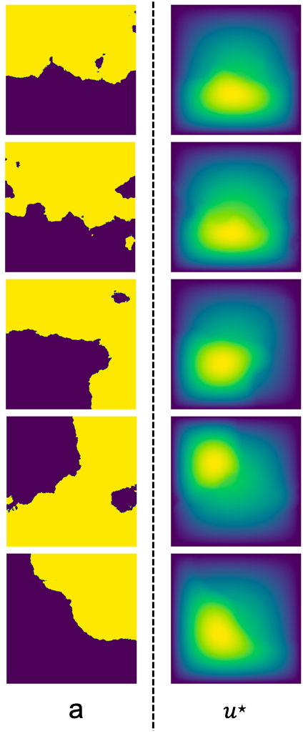
For our first set of experiments we consider stationary Darcy Flow equations, a form of linear elliptic PDE with in two dimensions. The PDE is defined as follows,
| (9) |
Note that the diffusion coefficient , i.e., the coefficients are always positive, and is the forcing term. These PDEs are used to model the steady-state pressure of fluids flowing through a porous media. They can also be used to model the stationary state of the diffusive process with modeling the temperature distribution through the space with defining the thermal conductivity of the medium. The task is to learn an operator such that .
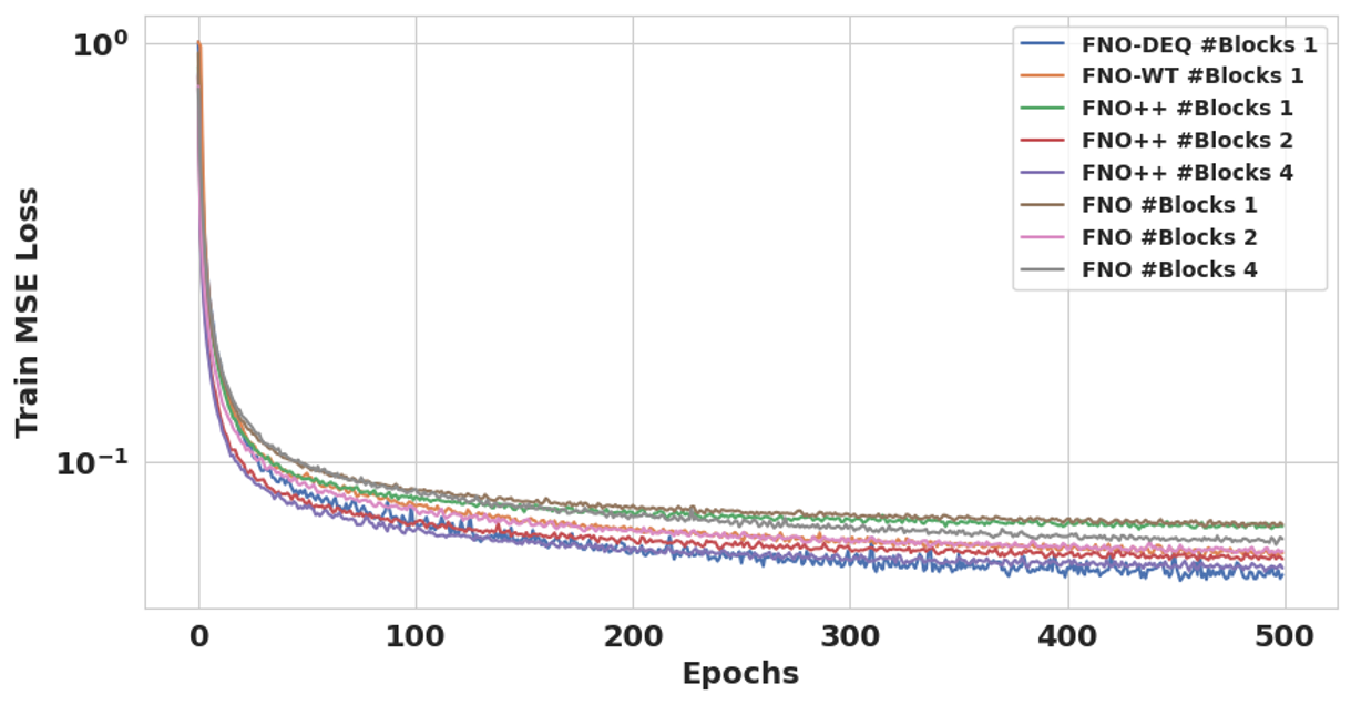
We report the results of our experiments on Darcy Flow in Table 8. The original FNO architecture does not improve its performance with increased number of FNO blocks . FNO++ with residual connections scales better but saturates at around 4 FNO blocks. In contrast, FNO-WT and FNO-DEQ with just a single FNO block outperform deeper non-weight-tied architectures on clean data and on data with noisy inputs. When observations are noisy, FNO-WT and FNO-DEQ outperform FNO++ with a similar number of parameters, and perform comparably to FNO++ with parameters.
We also report results on shallow FNO-DEQ, FNO-WT and FNO++ architectures. An FNO block in these shallow networks has a single FNO layer instead of three layers. In our experiments, shallow weight-tied networks outperform non-weight-tied architectures including FNO++ with parameters on clean data and on data with noisy inputs, and perform comparably to deep FNO++ on noisy observations. In case of noisy observations, we encounter training instability issues in FNO-DEQ. We believe that this shallow network lacks sufficient representation power and cannot accurately solve for the fixed point during the forward pass. These errors in fixed point estimation accumulate over time, leading to incorrect values of implicit gradients, which in turn result in training instability issues.
| Architecture | Parameters | #Blocks | Test error | ||
| FNO | 2.37M | 1 | 0.0080 5e-4 | 0.0079 2e-4 | 0.0125 4e-5 |
| FNO | 4.15M | 2 | 0.0105 6e-4 | 0.0106 4e-4 | 0.0136 2e-5 |
| FNO | 7.71M | 4 | 0.2550 2e-8 | 0.2557 8e-9 | 0.2617 2e-9 |
| FNO++ | 2.37M | 1 | 0.0075 2e-4 | 0.0075 2e-4 | 0.0145 7e-4 |
| FNO++ | 4.15M | 2 | 0.0065 2e-4 | 0.0065 9e-5 | 0.0117 5e-5 |
| FNO++ | 7.71M | 4 | 0.0064 2e-4 | 0.0064 2e-4 | 0.0109 5e-4 |
| S-FNO++ | 1.78M | 0.66 | 0.0093 5e-4 | 0.0094 7e-4 | 0.0402 6e-3 |
| FNO-WT | 2.37M | 1 | 0.0055 1e-4 | 0.0056 5e-5 | 0.0112 4e-4 |
| FNO-DEQ | 2.37M | 1 | 0.0055 1e-4 | 0.0056 7e-5 | 0.0112 4e-4 |
| S-FNO-WT | 1.19M | 0.33 | 0.0057 3e-5 | 0.0057 5e-5 | 0.0112 1e-4 |
| S-FNO-DEQ | 1.19M | 0.33 | 0.0056 4e-5 | 0.0056 5e-5 | 0.0136 0.011 |
5.2 Steady-state Navier-Stokes Equations for Incompressible Flow
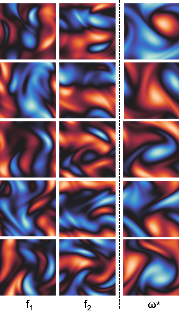
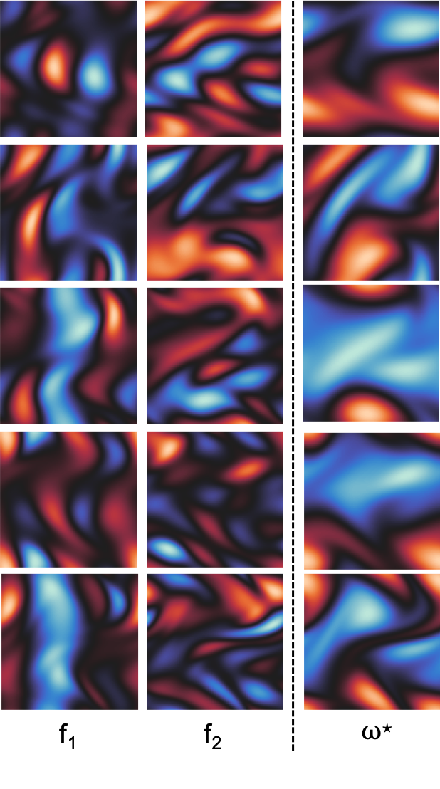
We consider the steady-state Navier-Stokes equation for an incompressible viscous fluid in the vorticity form defined on a torus, i.e., with periodic boundary condition,
| (10) |
where , and is the velocity and where , is the viscosity and is the external force term. We learn an operator , such that . We train all the models on data with viscosity values and , and create a dataset for steady-state incompressible Navier-Stokes, which we will make public as a community benchmark for steady-state PDE solvers.
Results for Navier-Stokes equation have been reported in Table 2 and Table 3. For both values of viscosity, FNO-DEQ outperforms other architectures for all three cases: clean data, noisy inputs and noisy observations. FNO-DEQ is more robust to noisy inputs compared to non-weight-tied architectures. For noisy inputs, FNO-DEQ matches the test-error of noiseless case in case of viscosity and almost matches the test-error of noiseless case in case of viscosity . We provide additional results for noise level in Appendix E. FNO-DEQ and FNO-WT consistently outperform non-weight-tied architectures for higher levels of noise as well.
In general, DEQ-based architectures are slower to train (upto 2.5 compared to feedforward networks of similar size) as we solve for the fixed point in the forward pass. However, their inductive bias provides performance gains that cannot be achieved by simply stacking non-weight-tied FNO layers. In general, we observe diminishing returns in FNO++ beyond 4 blocks. Additionally, training the original FNO network on more than 4 FNO blocks is challenging, with the network often diverging during training, and therefore we do not include these results in the paper.
| Architecture | Parameters | #Blocks | Test error | ||
|---|---|---|---|---|---|
| FNO | 2.37M | 1 | 0.184 0.002 | 0.218 0.003 | 0.184 0.001 |
| FNO | 4.15M | 2 | 0.162 0.024 | 0.176 0.004 | 0.152 0.005 |
| FNO | 7.71M | 4 | 0.157 0.012 | 0.187 0.004 | 0.166 0.013 |
| FNO++ | 2.37M | 1 | 0.199 0.001 | 0.230 0.001 | 0.197 0.001 |
| FNO++ | 4.15M | 2 | 0.154 0.005 | 0.173 0.003 | 0.154 0.006 |
| FNO++ | 7.71M | 4 | 0.151 0.003 | 0.165 0.004 | 0.149 0.003 |
| FNO-WT | 2.37M | 1 | 0.151 0.007 | 0.173 0.017 | 0.126 0.027 |
| FNO-DEQ | 2.37M | 1 | 0.128 0.004 | 0.144 0.007 | 0.136 0.003 |
| Architecture | Parameters | #Blocks | Test error | ||
|---|---|---|---|---|---|
| FNO | 2.37M | 1 | 0.181 0.005 | 0.186 0.003 | 0.178 0.006 |
| FNO | 4.15M | 2 | 0.138 0.007 | 0.150 0.006 | 0.137 0.012 |
| FNO | 7.71M | 4 | 0.152 0.006 | 0.163 0.002 | 0.151 0.008 |
| FNO++ | 2.37M | 1 | 0.188 0.002 | 0.207 0.004 | 0.187 0.003 |
| FNO++ | 4.15M | 2 | 0.139 0.004 | 0.153 0.002 | 0.140 0.005 |
| FNO++ | 7.71M | 4 | 0.130 0.005 | 0.151 0.004 | 0.128 0.009 |
| FNO-WT | 2.37M | 1 | 0.099 0.007 | 0.101 0.007 | 0.130 0.044 |
| FNO-DEQ | 2.37M | 1 | 0.088 0.006 | 0.099 0.007 | 0.116 0.011 |
6 Universal Approximation and Fast Convergence of FNO-DEQ
Though the primary contribution of our paper is empirical, we show (by fairly standard techniques) that FNO-DEQ is a universal approximator, under mild conditions on the steady-state PDEs. Moreover, we also show that in some cases, we can hope the fixed-point solver can converge rapidly.
As noted in Definition 2, we have . We note that all continuous function and can be written as, . where are the Fourier coefficients of the function . We define as as the space of functions such that for all with Fourier coefficients that vanish outside a bounded ball. Finally, we define an orthogonal projection operator , such that for all we have,
| (11) |
That is, the projection operator takes an infinite dimensional function and projects it to a finite dimensional space. We prove the following universal approximation result:
Theorem 1.
Let define the solution to a steady-state PDE in Definition 2, Then there exists an operator such that, . Furthermore, for every there exists an such that for compact sets and there exists a neural network with parameters , such that,
The proof for the above theorem is relatively straightforward and provided in Appendix C. The proof uses the fact that is a fixed-point of the operator , allowing us to use the the results in Kovachki et al. (2021a) that show a continuous operator can be approximated by a network as defined in Equation 2. Note that the choice of is by no means unique: one can “universally approximate” any operator , for a continuous operator . Such a can be thought of as a form of “preconditioned” gradient descent, for a preconditioner . For example, a Newton update has the form , where is the Frechet derivative of the operator .
The reason this is relevant is that the DEQ can choose to universally approximate a fixed-point equation for which the fixed-point solver it is trained with also converges rapidly. As an example, the following classical result shows that under Lax-Milgram-like conditions (a kind of strong convexity condition), Newton’s method converges doubly exponentially fast:
Lemma 1 (Faragó and Karátson (2002), Chapter 5).
Consider the PDE defined Definition 2, such that . such that defines the Frechet derivative of the operator . If for all we have and for , then for the Newton update, with , there exists an , such that if
For completeness, we include the proof of the above lemma in the Appendix (Section D). We note that the conditions of the above lemma are satisfied for elliptic PDEs like Darcy Flow, as well as many variational non-linear elliptic PDEs (e.g., those considered in Marwah et al. (2022)). Hence, we can expect FNO-DEQs to quickly converge to the fixed point, since they employ quasi-Newton methods like Broyden and Anderson methods (Broyden, 1965; Anderson, 1965).
7 Conclusion
In this work, we demonstrate that the inductive bias of deep equilibrium models—and weight-tied networks in general—makes them ideal architectures for approximating neural operators for steady-state PDEs. Our experiments on steady-state Navier-Stokes equation and Darcy flow equations show that weight-tied models and FNO-DEQ perform outperform FNO models with the number of parameters and depth. Our findings indicate that FNO-DEQ and weight-tied architectures are, in general, more robust to both input and observation noise compared to non-weight-tied architectures, including FNO. We believe that our results complement any future progress in the design and development of PDE solvers (Tran et al., 2021; Li et al., 2022b) for steady-state PDEs, and hope that our work motivates the study of relevant inductive biases that could be used to improve them.
8 Acknowledgements
TM is supported by CMU Software Engineering Institute via Department of Defense under contract FA8702-15-D-0002. AP is supported by a grant from the Bosch Center for Artificial Intelligence. ZL gratefully acknowledges the NSF (FAI 2040929 and IIS2211955), UPMC, Highmark Health, Abridge, Ford Research, Mozilla, the PwC Center, Amazon AI, JP Morgan Chase, the Block Center, the Center for Machine Learning and Health, and the CMU Software Engineering Institute (SEI) via Department of Defense contract FA8702-15-D-0002, for their generous support of ACMI Lab’s research. JL is supported in part by NSF award DMS-2012286, and AR is supported in part by NSF awards IIS-2211907, CCF-2238523, Amazon Research Award, and the CMU/PwC DT&I Center.
References
- Anderson (1965) Donald G Anderson. Iterative procedures for nonlinear integral equations. Journal of the ACM (JACM), 1965.
- Anil et al. (2022) Cem Anil, Ashwini Pokle, Kaiqu Liang, Johannes Treutlein, Yuhuai Wu, Shaojie Bai, J Zico Kolter, and Roger B Grosse. Path independent equilibrium models can better exploit test-time computation. Advances in Neural Information Processing Systems, 35:7796–7809, 2022.
- Bai et al. (2019) Shaojie Bai, J Zico Kolter, and Vladlen Koltun. Deep equilibrium models. Advances in Neural Information Processing Systems, 32, 2019.
- Bar-Sinai et al. (2019) Yohai Bar-Sinai, Stephan Hoyer, Jason Hickey, and Michael P Brenner. Learning data-driven discretizations for partial differential equations. Proceedings of the National Academy of Sciences, 116(31):15344–15349, 2019.
- Batchelor and Batchelor (1967) Cx K Batchelor and George Keith Batchelor. An introduction to fluid dynamics. Cambridge university press, 1967.
- Bhattacharya et al. (2021) Kaushik Bhattacharya, Bamdad Hosseini, Nikola B Kovachki, and Andrew M Stuart. Model reduction and neural networks for parametric PDEs. The SMAI journal of computational mathematics, 7:121–157, 2021.
- Boyd (2001) John P Boyd. Chebyshev and Fourier spectral methods. Courier Corporation, 2001.
- Brandstetter et al. (2022) Johannes Brandstetter, Daniel Worrall, and Max Welling. Message passing neural pde solvers. arXiv preprint arXiv:2202.03376, 2022.
- Broyden (1965) Charles G Broyden. A class of methods for solving nonlinear simultaneous equations. Mathematics of computation, 1965.
- Chen and Chen (1995) Tianping Chen and Hong Chen. Universal approximation to nonlinear operators by neural networks with arbitrary activation functions and its application to dynamical systems. IEEE Transactions on Neural Networks, 6(4):911–917, 1995.
- Chen et al. (2021) Ziang Chen, Jianfeng Lu, and Yulong Lu. On the representation of solutions to elliptic pdes in barron spaces. Advances in neural information processing systems, 34:6454–6465, 2021.
- Dresdner et al. (2022) Gideon Dresdner, Dmitrii Kochkov, Peter Norgaard, Leonardo Zepeda-Núñez, Jamie A. Smith, Michael P. Brenner, and Stephan Hoyer. Learning to correct spectral methods for simulating turbulent flows. 2022. doi: 10.48550/ARXIV.2207.00556. URL https://arxiv.org/abs/2207.00556.
- Faragó and Karátson (2002) István Faragó and János Karátson. Numerical solution of nonlinear elliptic problems via preconditioning operators: Theory and applications, volume 11. Nova Publishers, 2002.
- Fung et al. (2022) Samy Wu Fung, Howard Heaton, Qiuwei Li, Daniel McKenzie, Stanley Osher, and Wotao Yin. Jfb: Jacobian-free backpropagation for implicit networks. In Proceedings of the AAAI Conference on Artificial Intelligence, volume 36, pages 6648–6656, 2022.
- Geng et al. (2021) Zhengyang Geng, Xin-Yu Zhang, Shaojie Bai, Yisen Wang, and Zhouchen Lin. On training implicit models. Advances in Neural Information Processing Systems, 34:24247–24260, 2021.
- Hao et al. (2023) Zhongkai Hao, Zhengyi Wang, Hang Su, Chengyang Ying, Yinpeng Dong, Songming Liu, Ze Cheng, Jian Song, and Jun Zhu. Gnot: A general neural operator transformer for operator learning. In International Conference on Machine Learning, pages 12556–12569. PMLR, 2023.
- Hendrycks and Gimpel (2016) Dan Hendrycks and Kevin Gimpel. Gaussian error linear units (gelus). arXiv preprint arXiv:1606.08415, 2016.
- Hornik et al. (1989) Kurt Hornik, Maxwell Stinchcombe, and Halbert White. Multilayer feedforward networks are universal approximators. Neural networks, 2(5):359–366, 1989.
- Hsieh et al. (2019) Jun-Ting Hsieh, Shengjia Zhao, Stephan Eismann, Lucia Mirabella, and Stefano Ermon. Learning neural pde solvers with convergence guarantees. arXiv preprint arXiv:1906.01200, 2019.
- Kochkov et al. (2021) Dmitrii Kochkov, Jamie A Smith, Ayya Alieva, Qing Wang, Michael P Brenner, and Stephan Hoyer. Machine learning–accelerated computational fluid dynamics. Proceedings of the National Academy of Sciences, 118(21):e2101784118, 2021.
- Kopriva (2009) David A Kopriva. Implementing spectral methods for partial differential equations: Algorithms for scientists and engineers. Springer Science & Business Media, 2009.
- Kovachki et al. (2021a) Nikola Kovachki, Samuel Lanthaler, and Siddhartha Mishra. On universal approximation and error bounds for Fourier neural operators. The Journal of Machine Learning Research, 22(1):13237–13312, 2021a.
- Kovachki et al. (2021b) Nikola Kovachki, Zongyi Li, Burigede Liu, Kamyar Azizzadenesheli, Kaushik Bhattacharya, Andrew Stuart, and Anima Anandkumar. Neural operator: Learning maps between function spaces. arXiv preprint arXiv:2108.08481, 2021b.
- Kovachki et al. (2023) Nikola Kovachki, Zongyi Li, Burigede Liu, Kamyar Azizzadenesheli, Kaushik Bhattacharya, Andrew Stuart, and Anima Anandkumar. Neural operator: Learning maps between function spaces with applications to PDEs. Journal of Machine Learning Research, 24(89):1–97, 2023.
- Lanthaler et al. (2022) Samuel Lanthaler, Siddhartha Mishra, and George E Karniadakis. Error estimates for deeponets: A deep learning framework in infinite dimensions. Transactions of Mathematics and Its Applications, 6(1):tnac001, 2022.
- LeVeque (2007) Randall J LeVeque. Finite difference methods for ordinary and partial differential equations: steady-state and time-dependent problems. SIAM, 2007.
- Li et al. (2022a) Zijie Li, Kazem Meidani, and Amir Barati Farimani. Transformer for partial differential equations’ operator learning. arXiv preprint arXiv:2205.13671, 2022a.
- Li et al. (2020a) Zongyi Li, Nikola Kovachki, Kamyar Azizzadenesheli, Burigede Liu, Kaushik Bhattacharya, Andrew Stuart, and Anima Anandkumar. Fourier neural operator for parametric partial differential equations. arXiv preprint arXiv:2010.08895, 2020a.
- Li et al. (2020b) Zongyi Li, Nikola Kovachki, Kamyar Azizzadenesheli, Burigede Liu, Kaushik Bhattacharya, Andrew Stuart, and Anima Anandkumar. Neural operator: Graph kernel network for partial differential equations. arXiv preprint arXiv:2003.03485, 2020b.
- Li et al. (2022b) Zongyi Li, Daniel Zhengyu Huang, Burigede Liu, and Anima Anandkumar. Fourier neural operator with learned deformations for pdes on general geometries. arXiv preprint arXiv:2207.05209, 2022b.
- Liao et al. (2018) Renjie Liao, Yuwen Xiong, Ethan Fetaya, Lisa Zhang, KiJung Yoon, Xaq Pitkow, Raquel Urtasun, and Richard Zemel. Reviving and improving recurrent back-propagation. In International Conference on Machine Learning, pages 3082–3091. PMLR, 2018.
- Liu et al. (2022) Xinliang Liu, Bo Xu, and Lei Zhang. Mitigating spectral bias for the multiscale operator learning with hierarchical attention. October 2022. URL http://arxiv.org/abs/2210.10890.
- Lu et al. (2019) Lu Lu, Pengzhan Jin, and George Em Karniadakis. Deeponet: Learning nonlinear operators for identifying differential equations based on the universal approximation theorem of operators. arXiv preprint arXiv:1910.03193, 2019.
- Marwah et al. (2021) Tanya Marwah, Zachary Lipton, and Andrej Risteski. Parametric complexity bounds for approximating PDEs with neural networks. Advances in Neural Information Processing Systems, 34:15044–15055, 2021.
- Marwah et al. (2022) Tanya Marwah, Zachary C Lipton, Jianfeng Lu, and Andrej Risteski. Neural network approximations of PDEs beyond linearity: Representational perspective. arXiv preprint arXiv:2210.12101, 2022.
- Moukalled et al. (2016) Fadl Moukalled, Luca Mangani, Marwan Darwish, F Moukalled, L Mangani, and M Darwish. The finite volume method. Springer, 2016.
- Patankar and Spalding (1983) Suhas V Patankar and D Brian Spalding. A calculation procedure for heat, mass and momentum transfer in three-dimensional parabolic flows. In Numerical prediction of flow, heat transfer, turbulence and combustion, pages 54–73. Elsevier, 1983.
- Patel et al. (2021) Ravi G Patel, Nathaniel A Trask, Mitchell A Wood, and Eric C Cyr. A physics-informed operator regression framework for extracting data-driven continuum models. Computer Methods in Applied Mechanics and Engineering, 373:113500, 2021.
- Revay et al. (2020) Max Revay, Ruigang Wang, and Ian R Manchester. Lipschitz bounded equilibrium networks. arXiv preprint arXiv:2010.01732, 2020.
- Tran et al. (2021) Alasdair Tran, Alexander Mathews, Lexing Xie, and Cheng Soon Ong. Factorized Fourier neural operators. arXiv preprint arXiv:2111.13802, 2021.
- Winston and Kolter (2020) Ezra Winston and J Zico Kolter. Monotone operator equilibrium networks. Advances in neural information processing systems, 33:10718–10728, 2020.
Appendix
Appendix A Implementation Details
Training details.
We train all the networks for 500 epochs with Adam optimizer. The learning rate is set to 0.001 for Darcy flow and 0.005 for Navier-Stokes. We use learning rate weight decay of 1e-4 for both Navier-Stokes and Darcy flow. The batch size is set to 32. In case of Darcy flow, we also use cosine annealing for learning rate scheduling. We run all our experiments on a combination of NVIDIA RTX A6000, NVIDIA GeForce RTX 2080 Ti and 3080 Ti. All networks can easily fit on a single NVIDIA RTX A6000, but training time varies between the networks.
For FNO-DEQ, we use Anderson solver [Anderson, 1965] to solve for the fixed point in the forward pass. The maximum number of Anderson solver steps is kept fixed at 32 for Dary Flow, and 16 for Navier Stokes. For the backward pass, we use phantom gradients [Geng et al., 2021] which are computed as:
| (12) |
where is a tunable damping factor and is the fixed point computed using Anderson solver in the forward pass. This step can be repeated times. We use and for Darcy Flow, and and for Navier-Stokes.
For the S-FNO-DEQ used in Table 8, we use Broyden’s method [Broyden, 1965] to solve for the fixed point in the forward pass and use exact implicit gradients, computed through implicit function theorem as shown in Eq. 6, for the backward pass through DEQ. The maximum number of solver steps is fixed at 32.
For weight-tied networks, we repeatedly apply the FNO block to the input times for Darcy flow, and times for Navier-Stokes.
Network architecture details.
The width of an FNO layer set to 32 across all the networks. Additionally, we retain only 12 Fourier modes in FNO layer, and truncate higher Fourier modes. We use the code provided by Li et al. [2020a] to replicate the results for FNO, and construct rest of the networks on top of this as described in Sec. 5.
Appendix B Datasets
B.1 Darcy Flow
As mentioned in Sec. 5 we use the dataset provided by Li et al. [2020a] for our experiments with steady-state Darcy-Flow.
All the models are trained on 1024 data samples and tested on 500 samples. The resolution of original images is which we downsample to for our experiments. For experiments with noisy inputs/observations, the variance of Gaussian noise that we add to PDEs are [0, 1e-9, 1e-8, 1e-7, 1e-6, 1e-5, 1e-4, 1e-3].
B.2 Steady-State Incompressible Fluid Navier-Stoke
To generate the dataset for steady-state Navier-Stokes, instead of solving the steady state PDE using steady-state solvers like the SIMPLE algorithm Patankar and Spalding [1983], we first choose the solution of the PDE and then generate the corresponding equation, i.e. calculate the corresponding force term
To generate the solutions , we forward propagate a relatively simple initial distribution of (sampled from a Gaussian random field) through a time-dependent Navier-Stokes equation in the vorticity form for a short period of time. This ensures our dataset contains solutions that are rich and complex. Precisely, recall the Navier-Stokes equations in their vorticity form:
| (13) |
where and is a divergence free forcing term and are the two coordinates of the input vector. We forward propagate the equations Equation 13 using a pseudo-spectral method using the functions provided in JAX-CFD [Kochkov et al., 2021, Dresdner et al., 2022] package. The initial vorticity is sampled from a Gaussian random field , which is then made divergence free. We forward propagate the Navier-Stokes equation in Equation 13 for time with to get , which we choose as the solution to the steady-state PDE in Equation 10, i.e, for Equation 10.
Subsequently, we use the stream function [Batchelor and Batchelor, 1967] to calculate by solving the Poisson equation in the Fourier domain. Furthermore, since we use the stream function to calculate , i.e., the different components of the force term.
We use training samples and testing samples. The input to the network is the vector field and we learn a map that outputs the vorticity . The resolution of grid used to generate the dataset is which we downsample to while training the models. For experiments with noisy inputs/observations, we consider two values of maximum variance of Gaussian noise: 1e-3 and 4e-3. The variances of the Gaussian noise that we add to the PDEs for the latter case are [0, 1e-9, 1e-8, 1e-7, 1e-6, 1e-5, 1e-4, 1e-3, 2e-3, 4e-3]. However, when conducting experiments with a variance of 1e-3, we exclude the last two values of variance from this list.
Appendix C Proof of Universal Approximation
The proof of the universal approximation essentially follows from the result on the universal approximation capabilities of FNO layers in Kovachki et al. [2021a], applied to . For the sake of completeness, we reitarate the key steps.
For simplicity, we will assume that . (The results straightforwardly generalize.) We will first establish some key technical lemmas and introduce some notation and definitions useful for the proof for Theorem 1.
Definition 7.
An operator is continuous at if for every , there exists a , such that for all with , we have .
First, we approximate the infinite dimensional operator by projecting the functions in to a finite-dimensional approximation , and considering the action of the operator on this subspace. The linear projection we use is the one introduced in Equation 11. More precisely we show the following result,
Lemma 2.
Given a continuous operator as defined in Equation 1, let us define an operator as . Then, for every there exists an such that for all in any compact set , the operator is an -approximation of , i.e., we have,
Proof.
Note that for an there exists an such that for all we have
Therefore, using the definition of we can bound the norm of the difference between and as follows,
We first bound the term as follows:
| (14) |
Since is continuous, for all compact sets , is compact as well. This is because: (1) for any , is finite; (2) for any , . Therefore, for every , there exists an such that
Substituting the above result in Equation 14, we have
| (15) |
Similarly, for all where is compact, we can bound Term as following,
| (16) |
Now, since and is a continuous operator, there exists a modulus of continuity (an increasing real valued function) , such that for all , we have
Hence for every there exists an such that,
Plugging these bounds in Equation 16, we get,
| (17) |
Therefore, combining Equation 15 and Equation 17 then for , there exists an , such that for all we have
| (18) |
Taking proves the claim. ∎
Proof of Theorem 1.
For Lemma 2 we know that there exists a finite dimensional projection for the operator , defined as such that for all we have
Now using the definition of we have
From Kovachki et al. [2021a], Theorem 2.4 we know that there exists an FNO network of the form defined in Equation 2 such that for all , where is a compact set, there exists an we have
| (19) |
Finally, note that from Lemma D.1 in Kovachki et al. [2021a], we have that for any , there exists an FNO layers and defined in Equation 3 such that
| (20) |
and
| (21) |
for and .
Therefore there exists an such that there is an FNO network where such that
| (22) |
Appendix D Fast Convergence for Newton Method
Definition 8 (Frechet Derivative in ).
For a continuous operator , the Frechet derivative at is a linear operator such that for all we have
Lemma 3.
Given the operator with Frechet derivative , such that for all , we have , then exists and we have, for all :
-
1.
.
-
2.
Proof.
Note that for all we have,
Taking , we have
For part , note that there exists a such that
∎
We now show the proof for Lemma 4. The proof is standard and can be found in Faragó and Karátson [2002], however we include the complete proof here for the sake of completeness.
We restate the Lemma here for the convenience of the reader.
Lemma 4 (Faragó and Karátson [2002], Chapter 5).
Consider the PDE defined Definition 2, such that . such that defines the Frechet derivative of the operator . If for all we have 121212We note that this condition is different from the condition on the inner-product in the submitted version of the paper, which had. . and for , then for the Newton update, with , there exists an , such that if 131313We note that this rate is different from the one in the submitted version of the paper.
Proof of Lemma 4.
Re-writing the updates in Lemma 4 as,
| (23) | ||||
| (24) |
Now, upper bounding for all we have,
where we use Equation 24 in the final step.
Taking norm on both sides and using the fact that , we have
Noting that for all , we have , and using the fact that for all we have,
where we use the result from Lemma 3 in the last step.
Therefore we have
Therefore, if
then we have
for
∎
Appendix E Additional experimental results
We provide additional results for Navier-Stokes equation for noisy inputs and observations in Table 4 and Table 5. For these experiments, the maximum variance of Gaussian noise added to inputs and observations is 0.004. We observe that weight-tied FNO and FNO-DEQ outperform non-weight-tied architectures.
| Architecture | Parameters | #Blocks | Test error | ||
|---|---|---|---|---|---|
| FNO | 2.37M | 1 | 0.184 0.002 | 0.238 0.008 | 0.179 0.004 |
| FNO | 4.15M | 2 | 0.162 0.024 | 0.196 0.011 | 0.151 0.010 |
| FNO | 7.71M | 4 | 0.157 0.012 | 0.216 0.002 | 0.158 0.009 |
| FNO++ | 2.37M | 1 | 0.199 0.001 | 0.255 0.002 | 0.197 0.004 |
| FNO++ | 4.15M | 2 | 0.154 0.005 | 0.188 0.006 | 0.157 0.006 |
| FNO++ | 7.71M | 4 | 0.151 0.003 | 0.184 0.008 | 0.147 0.004 |
| FNO-WT | 2.37M | 1 | 0.151 0.007 | 0.183 0.026 | 0.129 0.018 |
| FNO-DEQ | 2.37M | 1 | 0.128 0.004 | 0.159 0.005 | 0.121 0.015 |
indicates that the network diverges during training for one of the seeds.
| Architecture | Parameters | #Blocks | Test error | ||
|---|---|---|---|---|---|
| FNO | 2.37M | 1 | 0.181 0.005 | 0.207 0.003 | 0.178 0.008 |
| FNO | 4.15M | 2 | 0.138 0.007 | 0.163 0.003 | 0.137 0.006 |
| FNO | 7.71M | 4 | 0.152 0.006 | 0.203 0.055 | 0.151 0.008 |
| FNO++ | 2.37M | 1 | 0.188 0.002 | 0.217 0.001 | 0.187 0.005 |
| FNO++ | 4.15M | 2 | 0.139 0.004 | 0.170 0.005 | 0.138 0.005 |
| FNO++ | 7.71M | 4 | 0.130 0.005 | 0.168 0.007 | 0.126 0.007 |
| FNO-WT | 2.37M | 1 | 0.099 0.007 | 0.159 0.029 | 0.123 0.023 |
| FNO-DEQ | 2.37M | 1 | 0.088 0.006 | 0.104 0.001 | 0.116 0.005 |
indicates that the network diverges during training for one of the seeds.
Convergence analysis of fixed point.
We report variations in test error, absolute residual , and relative residual with an increase in the number of solver steps while solving for the fixed point in FNO-DEQ, for both Darcy Flow (See Table 6) and Steady-State Navier Stokes (See Table 7). We observe that all these values decrease with increase in the number of fixed point solver iterations and eventually saturate once we have a reasonable estimate of the fixed point. We observe that increasing the number of fixed point solver iterations results in a better estimation of the fixed point. For steady state PDEs, we expect the test error to reduce as the estimation of the fixed point improves. Furthermore, at inference time we observe that the test error improves (i.e. reduces) with increase in the number of fixed point solver iterations even though the FNO-DEQ is trained with fewer solver steps. For Navier-Stokes with viscosity 0.01, at inference time we get a test MSE loss of 0.0744 with 48 solver steps from 0.0847 when used with 24 solver steps.
This further bolsters the benefits of DEQs (and weight-tied architectures in general) for training neural operators for steady-state PDEs. Moreover, performance saturates after a certain point once we have a reasonable estimate of the fixed point, hence showing that more solver steps stabilize to the same solution.
| Solver steps | Absolute residual | Relative residual | Test Error |
|---|---|---|---|
| 2 | 212.86 | 0.8533 | 0.0777 |
| 4 | 18.166 | 0.0878 | 0.0269 |
| 8 | 0.3530 | 0.00166 | 0.00567 |
| 16 | 0.00239 | 1.13e-5 | 0.00566 |
| 32 | 0.000234 | 1.1e-6 | 0.00566 |
| Solver steps | Absolute residual | Relative residual | Test Error |
|---|---|---|---|
| 4 | 544.16 | 0.542 | 0.926 |
| 8 | 397.75 | 0.408 | 0.515 |
| 16 | 150.33 | 0.157 | 0.147 |
| 24 | 37.671 | 0.0396 | 0.0847 |
| 48 | 5.625 | 0.0059 | 0.0744 |
| 64 | 3.3 | 0.0034 | 0.0746 |

| Architecture | Parameters | #Blocks | Test error | ||
|---|---|---|---|---|---|
| FNO | 2.37M | 1 | 0.0080 5e-4 | 0.0079 2e-4 | 0.0125 4e-5 |
| FNO | 4.15M | 2 | 0.0105 6e-4 | 0.0106 4e-4 | 0.0136 2e-5 |
| FNO | 7.71M | 4 | 0.2550 2e-8 | 0.2557 8e-9 | 0.2617 2e-9 |
| FNO++ | 2.37M | 1 | 0.0075 2e-4 | 0.0075 2e-4 | 0.0145 7e-4 |
| FNO++ | 4.15M | 2 | 0.0065 2e-4 | 0.0065 9e-5 | 0.0117 5e-5 |
| FNO++ | 7.71M | 4 | 0.0064 2e-4 | 0.0064 2e-4 | 0.0109 5e-4 |
| FNO-WT | 2.37M | 1 | 0.0055 1e-4 | 0.0056 5e-5 | 0.0112 4e-4 |
| FNO-DEQ | 2.37M | 1 | 0.0055 1e-4 | 0.0056 7e-5 | 0.0112 4e-4 |