Uncertainty in Graph Contrastive Learning
with Bayesian Neural Networks

Abstract

Graph contrastive learning has shown great promise when labeled data is scarce, but large unlabeled datasets are available. However, it often does not take uncertainty estimation into account. We show that a variational Bayesian neural network approach can be used to improve not only the uncertainty estimates but also the downstream performance on semi-supervised node-classification tasks. Moreover, we propose a new measure of uncertainty for contrastive learning, that is based on the disagreement in likelihood due to different positive samples.

1 Introduction

Traditional supervised learning with deep neural networks does not leverage the information contained in unlabeled data and performs poorly in scarce data settings. Partially as a response to this, self-supervised training methods for neural networks on graphs and images have seen great progress in recent years. Hereby, the InfoNCE objective introduced by Oord et al. (2018) has played an important part as it constitutes the basis for many of the best-performing methods that have been developed (Chen et al., 2020; He et al., 2020b; You et al., 2020; Zhu et al., 2020). This contrastive loss uses positive and negative examples for each data point and encourages the network to learn a function that maps the positives close to each other and the negatives further apart in an embedding space. Often, the positive samples are generated by creating augmentations of the original data point and the negative ones are taken to be random samples from the data.

For many application areas of contrastive learning, such as object detection (Xie et al., 2021) or drug discovery (Sanchez-Fernandez et al., 2022), obtaining accurate uncertainty estimates is essential. Nevertheless, research into probabilistic approaches to InfoNCE learning is limited. A notable exception is Aitchison and Ganev (2023), who have shown that the weights of the encoding neural network (encoder) can be learned by optimizing an evidence lower bound (ELBO). We extend this result to include distributions over the parameters and equip the model with a notion of (Bayesian) epistemic uncertainty. Related to this, we make the following contributions:

1. We propose variational graph constrastive learning (VGCL) and find that regularizing the variational family leads to a remarkable improvement in downstream accuracy.

2. We investigate the uncertainty calibration on a downstream task with respect to different existing uncertainty measures. We find all the measures to be improved when VGCL is used and weight uncertainty is taken into account.

3. We propose the contrastive model disagreement score (CMDS), a new approach for measuring uncertainty in contrastive learning based on the disagreement between positive samples. We empirically show that it outperforms the currently used measures.

2 Background

2.1 Deep Learning on Graphs

Deep learning on graphs aims to develop neural network models for graph-structured data. Graph Neural Networks (GNNs) leverage convolutional filters to process the information contained in nodes and edges to extract meaningful features and predict graph properties (Gama et al., 2020; Wu et al., 2020). The problem setting which we investigate is node classification. Here, the observed data is one input graph consisting of $n$ nodes with node features $\vec{X}\in\mathbb{R}^{n\times f}$ and an adjacency matrix $\vec{A}\in\mathbb{R}^{n\times n}$. In the self-supervised setting, we aim to train a network that maps the observed data on this manifold into the Euclidean space $\mathbb{R}^{m}$ in a way that results in a useful node embedding. The quality of these embeddings is evaluated via a linear classifier trained on the node labels.

2.2 Self-Supervised Learning with the InfoNCE

The InfoNCE (Oord et al., 2018) considers two data items $x$ and $x^{\prime}$, where $x$ could be the original data point or anchor and $x^{\prime}$ could be an augmentation of $x$. These data points are mapped by an encoder $\mathrm{Q}_{\phi}(z\mid x)$ to their respective embeddings $z$ and $z^{\prime}$. Here, $\phi$ are the parameters of the encoder. The InfoNCE objective is then defined as:

$$\mathrm{I}_{N}(\phi,\rho)=\operatorname{\mathbb{E}}_{X}\left(\log\frac{f_{\rho}(z,z^{\prime})}{f_{\rho}(z,z^{\prime})+\sum_{j=1}^{N}f_{\rho}(z,z_{j})}\right)+\log(N)$$ (1)

where $z_{j}$ are the embeddings of $N$ negative examples and $f_{\rho}(\cdot,\cdot)$ is a similarity function, parameterised by $\rho$, that is used to distinguish the samples in the embedding space. Usually it is taken to be the cosine similarity coupled with an additional MLP layer called the projection head.

2.3 A Probabilistic Interpretation of the InfoNCE

Recently, Aitchison and Ganev (2023) have shown that contrastive learning can be interpreted as a generative process and have formulated a related statistical model. In this setting, pairs of data points $x$, $x^{\prime}$ are observed that are generated by the latent variables $z$ and $z^{\prime}$. The likelihood $\mathrm{P}_{\phi,\rho}\left(x,x^{\prime}\right)$ is a joint distribution over the observed data and it is parametrised by ($\phi$, $\rho$). The model parameters that maximize the corresponding model evidence can then be approximately found by optimizing the following evidence lower bound (further details in Appendix B):

$$\log\mathrm{P}_{\phi,\rho}\left(x,x^{\prime}\right)\geq\mathbb{E}_{\mathrm{Q}_{\phi}\left(z,z^{\prime}\mid x,x^{\prime}\right)}\left[\log\frac{\mathrm{P}_{\theta,\rho}\left(z,z^{\prime}\right)}{\mathrm{Q}_{\phi}\left(z^{\prime}\right)\mathrm{Q}_{\phi}\left(z\right)}\right]+\log\mathrm{P}_{true}(x)\mathrm{P}_{true}(x^{\prime})$$ (2)

where $\mathrm{Q}_{\phi}\left(z\right)$ and $\mathrm{Q}_{\phi}\left(z^{\prime}\right)$ are the marginals of the joint distribution $\mathrm{Q}_{\phi}\left(z,z^{\prime}\right)$. Hereby, the true distributions do not depend on the parameters of the model and we can optimize the bound without taking them into consideration. Moreover, $\mathrm{P}_{\phi,\rho}\left(z,z^{\prime}\right)$ is a prior over the latent variables. It turns out that when we choose it as $\mathrm{P}_{\phi,\rho}\left(z,z^{\prime}\right)=\mathrm{P}_{\phi,\rho}\left(z\right)\,\mathrm{P}_{\phi,\rho}\left(z^{\prime}\mid z\right)$ and pick:

$$\mathrm{P}_{\phi,\rho}(z) =\mathrm{Q}_{\phi}(z)$$ (3)

$$\mathrm{P}_{\phi,\rho}\left(z^{\prime}\mid z\right) =\frac{1}{Z_{\phi,\rho}(z)}\mathrm{Q}_{\phi}\left(z^{\prime}\right)f_{\rho}\left(z,z^{\prime}\right)$$

with $Z_{\phi,\rho}(z)$ being a normalizing constant, then we obtain an objective that is equivalent to the InfoNCE (up to a constant) for a deterministic encoder (Appendix C). A more detailed treatment of the related work is deferred to Appendix G.

3 Methods

3.1 VGCL: Contrastive Learning with Probabilistic Encoders

To obtain a model that accounts for the epistemic uncertainty in the parameters, we alter the formulation of the evidence lower bound for contrastive learning to include a distribution over the weights $w=(\phi,\rho)$. This yields a Variational Graph Contrastive Learning (VGCL) approach. The related ELBO (Appendix B) that we would like to optimize is:

$$\log\mathrm{P}\left(x,x^{\prime}\right)\geq\mathbb{E}_{\mathrm{Q}\left(z,z^{\prime}\mid x,x^{\prime},w\right)\mathrm{q}(w\mid\theta)}\left[\log\frac{\mathrm{P}\left(z,z^{\prime}\mid w\right)}{\mathrm{Q}\left(z^{\prime}\mid w\right)\mathrm{Q}\left(z^{\prime}\mid w\right)}\right]-KL(\mathrm{q}(w\mid\theta)\,\|\,\mathrm{P}(w))$$ (4)

where the last term is the Kullback–Leibler divergence between the prior over the weights $P(w)$ and the variational family $q(w\mid\mathbf{\theta})$ parametrised by $\theta$. For our experiments, we pick them to be Gaussian distributions. We thus have $P(w)=\prod_{j}\mathcal{N}\left(w_{j}\mid\mu,\sigma^{2}\right)$ and $q(w\mid\mathbf{\theta})=\prod_{j}\mathcal{N}\left(w_{j}\mid\mathbf{\theta}\right)$ where each $w_{j}$ is a weight of the neural network. Furthermore, following Blundell et al. (2015), we reparameterize the standard deviation of the variational distribution as $\sigma_{v}=\log(1+\exp(p))$ and the parameter set is thus $\theta=(\mu,p)$. In addition to that, we regularize the variational family by placing Gaussian hyperpriors over the variational parameters:

$$\mu_{v}\sim\mathcal{N}(0,\sigma_{0}^{2})\,,\,p\sim\mathcal{N}(\mu_{p},\sigma_{p}^{2})$$ (5)

This is meant to encourage a larger variance in the weights, due to the fact that we are training the model on augmentations, which are only an approximation to the data that would be the result of a generating process given the true latents. We thus hypothesize that a larger uncertainty about the model weights might be beneficial and we incorporate this prior knowledge by regularizing the variational family.

3.2 CMDS: Uncertainty in Contrastive Learning

Existing works on uncertainty in contrastive learning either do not model the uncertainty related to a data point $x$ explicitly or focus on its embedding uncertainty (Appendix G). That is, they use a trained encoder to map $x$ into the embedding space and then reason about the variance of the embedding features (e.g. under different augmentations). Instead, we use the probabilistic model of the InfoNCE to design a measure of uncertainty that is related to the likelihood of the data and incorporates the epistemic uncertainty of the weight distribution when using a BNN. To this end, we note that the likelihood in the probabilistic model of contrastive learning is the contrastive loss and that it is calculated based on $x$ and $x^{\prime}$. Thus, in contrast to other works, we encode two data points and reason about the quantity $\mathrm{P}_{\theta,\rho}(x,x^{\prime})$.

Table 1: Test accuracies for different unsupervised methods on the citation datasets. Our proposed method outperforms all the baselines on all tasks.

Dataset	Cora	Citeseer	Pubmed
Raw features	$64.8$	$64.6$	$84.8$
node2vec	74.8	52.3	$80.3$
DeepWalk	75.7	50.5	$80.5$
Deep Walk + Features	$73.1$	$47.6$	$83.7$
GAE	$76.9$	$60.6$	$82.9$
VGAE	$78.9$	$61.2$	$83.0$
DGI	$82.6\pm 0.4$	$68.8\pm 0.7$	$86.0\pm 0.1$
InfoNCE	$81.9\pm 0.4$	$70.8\pm 0.1$	$85.0\pm 0.1$
VI-InfoNCE	$82.1\pm 0.3$	$71.0\pm 0.1$	$85.0\pm 0.1$
VGCL (Ours)	$\mathbf{83.5\pm 0.2}$	$\mathbf{72.2\pm 0.1}$	$\mathbf{86.3\pm 0.1}$

To incorporate the contrastive nature of the problem, we propose to quantify the uncertainty of $x$ by using the variation of $\mathrm{P}_{\theta,\rho}(x\mid x^{\prime})$ under samples $x^{\prime}\sim p(x^{\prime}\mid z^{\prime})$. The intuition is that for a data point and context for which the model has learned a coherent explanation, it will assign similar likelihoods for different positive examples. The samples can be obtained by creating augmentations of $x$.

Notably, a related idea exists in out-of-distribution detection for Bayesian Variational Autoencoders, where Daxberger and Hernández-Lobato (2019) measure the disagreement in the likelihood estimates of different models sampled from a learned weight distribution. Extending their idea to contrastive learning, we calculate the related disagreement score not only for weights but also for positive samples. This leads to the Contrastive Model Disagreement Score (CMDS):

$$D_{\text{CMDS}}\left(x\right)=\frac{1}{M\sum_{j=1}^{M}l_{j}(x)^{2}}\,\qquad\text{with}\quad l_{j}(x)=\frac{\mathrm{P}\left(x\mid x^{\prime}_{j},\phi_{j},\rho_{j}\right)}{\sum_{j=1}^{M}\mathrm{P}\left(x\mid x^{\prime}_{j},\phi_{j},\rho_{j}\right)},$$ (6)

where we generate $M$ samples from $x^{\prime}_{j}\sim p(x\mid z^{\prime})$ via augmentations and $\rho_{j},\phi_{j}\sim q(w\mid\theta)$ from the learned variational families. This score will be large when the normalised likelihoods $l_{j}$ are alike and small when they differ a lot. It is important to emphasize that, while the mathematical formulation of the CMDS is similar to the measure proposed by Daxberger and Hernández-Lobato (2019) there are some fundamental differences. Importantly, the CMDS can be applied to deterministic models and it is based on the joint likelihood between $x,x^{\prime}$ that is inherent to contrastive learning. The measure proposed by Daxberger and Hernández-Lobato (2019) can only be used for Bayesian models and it is defined for the setting where a Variational Autoencoder is trained with a reconstruction loss. There, the likelihood is only based on one data point. For an extended discussion and mathematical explanation of the CMDS we defer the reader to Appendices D and E.

4 Experiments

fig:tsns

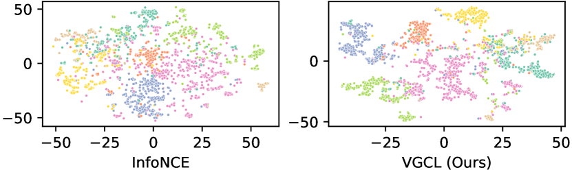
Figure 1: T-SNE plots of the embeddings generated by a deterministic encoder (left) in comparison to the embeddings generated by our probabilistic encoder with hyperpriors (right). Our method generates a better separation between the classes in the embedding spaces, which might explain its improved performance.

We evaluate the proposed methods on the Planetoid citation datasets for node classification (Appendix A). We use a standard transductive set-up for SSL to evaluate the methods (Zhu et al., 2021). That is, we train the self-supervised learner on all available data points and afterwards fit a linear classifier on the obtained embeddings. A 10/10/80 split is used and the embeddings are evaluated with the mean test accuracy over different data splits. To compare the usefulness of the generated (unsupervised) uncertainty estimates we use the resulting retention curves of the linear classifier on the test set. Unless specified otherwise, we report the mean and standard error estimates based on 20 runs.

Probabilistic Encoders

On all datasets, an encoder with Gaussian priors performs on-par or slightly better than its deterministic counterpart (Table 1). In addition to that, we find that using variational graph contrastive learning with hyperpriors (VGCL) yields significant performance improvements of up to $1.3$ percent points. A visualization of the created embeddings with a T-SNE plot shows that these improvements in accuracy stem from a better separation of the embedding space (LABEL:fig:tsns). We also find that setting a hyperprior on the variance of the variational family leads to much better uncertainty estimates. (LABEL:fig:ret_curves, right).

Representation Uncertainty

fig:ret_curves

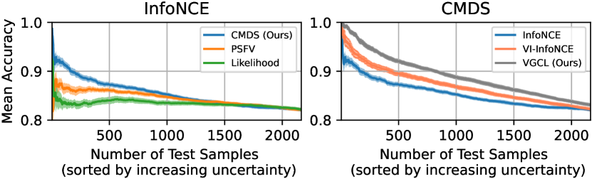
Figure 2: (Left) Error retention curves on Cora for different uncertainty measures for a deterministic InfoNCE model. We see that our proposed uncertainty measure yields the best sorting. (Right) Performance of the CMDS for different models. We see that the uncertainty calibration improves when Bayesian weight uncertainty is taken into account. To generate the plots, the test data is ordered by increasing uncertainty and the accuracy is calculated as gradually more test samples are incorporated. For a good uncertainty measure the mean accuracy is high for the most certain samples and decreases as more uncertain data points are included.

For the trained models, we calculate the average standard deviation of the embedding features (ASTD, Hasanzadeh et al., 2021), the min-max normalized ASTD, the Per-Feature-Sample-Variance (Ardeshir and Azizan, 2022), the expected likelihood under positive samples $\mathbb{E}_{x^{\prime}\sim p(x\mid z^{\prime})}\left[\mathrm{P}_{\theta,\rho}(x\mid x^{\prime})\right]$, the related Watanabe-Akaike Information Criterion (WAIC) $\mathbb{E}_{x^{\prime}\sim p(x\mid z^{\prime})}\left[\mathrm{P}_{\theta,\rho}(x\mid x^{\prime})\right]-\mathrm{Var}_{x^{\prime}\sim p(x\mid z^{\prime})}\left[\log\mathrm{P}_{\theta,\rho}\left(x\mid x^{\prime}\right)\right]$, and the CMDS under positive samples as proposed in Section 3.2. We consider all scores with and without uncertainty in the weights. We illustrate some representative results in LABEL:fig:ret_curves and show additional ones in Appendix F. We observe that our proposed uncertainty measure yields the best correlation with downstream predictive accuracy of all the considered criteria (LABEL:fig:ret_curves, left) and we also see that our proposed method provides the best uncertainties (LABEL:fig:ret_curves, right).

5 Conclusion

We have proposed VGCL, a variational Bayesian approach to graph contrastive learning, and CMDS, a novel measure for uncertainty in the learned representations. We have shown that VGCL yields better downstream performance than the baseline methods on all investigated graph datasets and that it yields uncertainties that are better calibrated. Moreover, we have shown that CMDS correlates better with downstream accuracy than other criteria from the literature. In future work, it would be interested to study whether different priors or variational distributions could additionally improve the performance of VGCL and whether the superior uncertainty estimation of the combination of VGCL with CMDS transfers from the graph setting onto other modalities (e.g., images).

The work of Elvin Isufi is supported by the TU Delft AI Labs programme. Alexander Immer is supported by a Max Planck ETH Center for Learning Systems doctoral fellowship. Vincent Fortuin was supported by a Branco Weiss Fellowship.

Appendix A Experimental Details

Datasets

We utilize three widely-used citation networks, Cora, Citeseer, Pubmed, for predicting article subject categories (Yang et al., 2016; Sen et al., 2008). The Cora dataset consists of 2708 scientific publications that constitute the nodes while CiteSeer is made up of 3327 and Pubmed of 19717. The edges are the citation links between the papers and the features are a sparse bag-of-words for each node.

Models

As encoder we use a two-layers GCN as proposed by Kipf and Welling (2016):

$$\mathrm{E}_{i}(\boldsymbol{X},\boldsymbol{A}) =\sigma\left(\hat{\boldsymbol{D}}^{-\frac{1}{2}}\hat{\boldsymbol{A}}\hat{\boldsymbol{D}}^{-\frac{1}{2}}\boldsymbol{X}\boldsymbol{W}_{i}\right)$$ (7)

$$Z(\boldsymbol{X},\boldsymbol{A}) =\mathrm{E}_{2}\left(\mathrm{E}_{1}(\boldsymbol{X},\boldsymbol{A}),\boldsymbol{A}\right).$$

where we use the adjacency matrix with self-loops $\hat{\boldsymbol{A}}=\boldsymbol{A}+\boldsymbol{I}$ and normalise with the degree matrix $\hat{\boldsymbol{D}}=\sum_{i}\hat{\boldsymbol{A}}_{i}$. For all models we use a hidden layer size of 128 and a ReLU activation function. In addition to that, we use two MLP layers with a hidden layer size of 128 and an ELU activation as projection head. We then calculate the cosine similarity of the output as similarity in the contrastive loss.

Training and Hyperparameters

We train all models for 150 epochs for the Cora and Citeseer datasets and for 1500 epochs for Pubmed and use Adam for parameter optimization (Kingma and Ba, 2014). Furthermore, we use the temperature-scaled InfoNCE loss as introduced by Chen et al. (2020) and applied to graphs by You et al. (2020). We average the loss over $20$ samples when training the probabilistic encoders. The data is augmented via a mix of feature masking and edge dropping as proposed by Zhu et al. (2020). We thus create graph augmentations by applying a Bernoulli dropout on the edges and features where we tune the respective probabilities. Following Zhu et al. (2021), during training we create two augmentations of the original graph and compare these via the contrastive loss. Hereby, we tune the Bernoulli dropout probabilities to create the two different augmentations separately resulting in the hyperparameters $p_{f,1},p_{e,1},p_{f,2},p_{e,2}$. We obtain the accuracies used in the paper with the hyperparameter settings in Table 2.

Dataset	Model	$p_{f,1}$	$p_{f,2}$	$p_{r,1}$	$p_{r,2}$	$\begin{array}[]{c}\text{ lr }\end{array}$	$\sigma^{2}$	$\sigma_{0}$	$\mu_{p}^{2}$	$\sigma_{p}^{2}$
Cora	VI-InfoNCE	0.3	0.3	0.4	0.4	$5*10^{-3}$	0.0025	-	-	-
Citeseer	VI-InfoNCE	0.3	0.4	0.4	0.4	$5*10^{-3}$	0.0010	-	-	-
Pubmed	VI-InfoNCE	0.0	0.2	0.4	0.1	$10^{-2}$	0.0100	-	-	-
Cora	VGCL	0.3	0.3	0.4	0.4	$10^{-2}$	0.0025	-	0	$10^{-6}$
CiteSeer	VGCL	0.3	0.4	0.4	0.4	$5*10^{-3}$	0.0010	0.001	$10^{-3}$	$10^{-3}$
Pubmed	VGCL	0.0	0.2	0.4	0.1	$10^{-2}$	0.0100	-	0	$10$

Table 2: Hyperparameters

Evaluation and Baselines

As we consider the transductive setting the models are trained on all the available unlabeled data in an unsupervised manner. Afterwards the epoch with the smallest contrastive loss is chosen and the created embeddings are evaluated by fitting a $l_{2}$-regularized logistic regression. Hereby, we follow Zhu et al. (2021) and use $10\%$ of the data for training, $10\%$ for validation and $80\%$ for testing. For the Bayesian Models we sample $100$ embeddings for each node and use the average feature values in the evaluation.

As baselines for the uncertainty quantification task we have considered the measures in the literature that are unsupervised and are directly calculatable for a trained InfoNCE learner (i.e not based on an additional model for density estimation such as a Gaussian-Mixture-Model). In addition to that, we note that the Per-Sample-Feature-Variation (PSFV, Ardeshir and Azizan, 2022) and the Average-Standard-Deviation of the features (ASTD, Hasanzadeh et al., 2021) are computationally very similar quantities. Nevertheless, in the PSFV the variation in the embeddings is a result of taking different augmentations, while in the ASTD the uncertainty comes from the distribution over the weights. Therefore, the ASTD score is not applicable to a deterministic encoder. Generally, when we calulate the uncertainty measures in our experiments, we use the contrastive loss to approximate the likelihood. In practice we use the objective that is being minimized but change the order as appropriate for the sorting of the retention curves. The acronyms in the results presented in Table 1 are Graph Autoencoder, Variational Graph Autoencoder (GAE,VGAE, Kipf and Welling, 2016) and Deep Graph Infomax (DGI, Veličković et al., 2019). We have implemented the InfoNCE, VI-InfoNCE and VGCL methods ourselves and have taken the results for the other ones from Zhu et al. (2020) where the same experimental procedure and datasets are used as in our work.

Appendix B Derivation of the ELBO for a probabilistic encoder

In this section, we step through the derivation of the ELBO that includes weight uncertainty in the encoders and in the projection head. When reading the derivation it is important to keep in mind, that the model proposed by Aitchison and Ganev (2023) has little similarity with a variational autoencoder that uses a reconstruction loss. The term variational autoencoder is used in the literal sense, that we learn by optimizing an evidence lower bound.

In the model we consider two separate encoders (usually we share weights and effectively train one neural network), one that encodes $x$ and the other one that encodes $x^{\prime}$. Thus, to be fully general, we have to consider the weights over the first network $\phi_{1}$, the weights over the second network $\phi_{2}$ and the weights in the similiarity function $\rho$ separately. For the following derivation we furthermore use that:

$$\mathrm{P}\left(x,x^{\prime},z,z^{\prime},\phi_{1},\phi_{2},\rho\right) =\mathrm{P}\left(x,x^{\prime},z,z^{\prime}\mid\phi_{1},\phi_{2},\rho\right)\mathrm{P}\left(\phi_{1},\phi_{2},\rho\right)$$ (8)

$$=\mathrm{P}\left(x|z,\phi_{1}\right)\mathrm{P}\left(x^{\prime}|z^{\prime},\phi_{2}\right)\mathrm{P}\left(z,z^{\prime}|,\phi_{1},\phi_{2},\rho\right)\mathrm{P}\left(\phi_{1},\phi_{2},\rho\right)$$ (9)

which is because the data is modeled as independent given the latents. The likelihoods are approximated with:

$$\mathrm{P}\left(x|z,\phi_{1}\right)=\frac{\mathrm{Q}(z\mid x,\phi_{1})\ \mathrm{P}_{\text{true }}\left(x\right)}{\mathrm{Q}(z|\phi_{1})}$$ (10)

$$\mathrm{P}\left(x^{\prime}|z^{\prime},\phi_{2}\right)=\frac{\mathrm{Q}(z^{\prime}\mid x^{\prime},\phi_{2})\ \mathrm{P}_{\text{true }}\left(x^{\prime}\right)}{\mathrm{Q}(z^{\prime}|\phi_{2})}$$ (11)

while this definition of the likelihoods might seem unfamiliar at first, it stems from the absence of a reconstruction loss and from the fact that the encoders are not invertible (for further details see Aitchison and Ganev (2023)). In addition, the approximate posterior for two data points decomposes as:

$$\mathrm{Q}(z,z^{\prime}\mid x,x^{\prime},\phi_{1}\ \phi_{2})=\mathrm{Q}(z\mid x,\phi_{1})\ \mathrm{Q}(z^{\prime}\mid x^{\prime},\phi_{2})$$ (12)

Then:

$$\log\mathrm{P}\left(x,x^{\prime}\right)$$ (13)

$$=\log\int d\phi_{1}\ d\phi_{2}\ d\rho\ dz\ dz^{\prime}\mathrm{P}\left(x,x^{\prime},z,z^{\prime},\phi_{1},\phi_{2},\rho\right)$$

$$=\log\int d\phi_{1}\ d\phi_{2}\ d\rho\ dz\ dz^{\prime}\mathrm{P}\left(x,x^{\prime},z,z^{\prime}\mid\phi_{1},\phi_{2},\rho\right)\mathrm{P}\left(\phi_{1},\phi_{2},\rho\right)$$

$$=\log\int d\phi_{1}\ d\phi_{2}\ d\rho\ dz\ dz^{\prime}\mathrm{Q}(z,z^{\prime}\mid x,x^{\prime},\phi_{1},\phi_{2})\ \mathrm{q}(\phi_{1},\phi_{2},\rho\mid\theta)\frac{\mathrm{P}\left(x,x^{\prime},z,z^{\prime}\mid\phi_{1},\phi_{2},\rho\right)\mathrm{P}\left(\phi_{1},\phi_{2},\rho\right)}{\mathrm{Q}(z,z^{\prime}\mid x,x^{\prime},\phi_{1}\ \phi_{2})\ \mathrm{q}(\phi_{1},\phi_{2},\rho\mid\theta)}$$

Identifying this as an expectation and plugging in the approximate likelihoods from above we get:

$$\log\mathrm{E}_{\mathrm{Q}\left(z,z^{\prime}\mid x,x^{\prime},\phi_{1},\phi_{2}\right)\mathrm{q}(\phi_{1},\phi_{2},\rho\mid\theta)}\left[\frac{\mathrm{Q}(z^{\prime}\mid x^{\prime},\phi_{2})\ \mathrm{P}_{\text{true }}\left(x^{\prime}\right)\mathrm{Q}(z\mid x,\phi_{1})\ \mathrm{P}_{\text{true }}\left(x\right)\mathrm{P}\left(z,z^{\prime}\mid\phi_{1},\phi_{2},\rho\right)\mathrm{P}\left(\phi_{1},\phi_{2},\rho\right)}{\mathrm{Q}(z,z^{\prime}\mid x,x^{\prime},\phi_{1}\ \phi_{2})\mathrm{Q}\left(z^{\prime}\mid\phi_{2}\right)\mathrm{Q}\left(z\mid\phi_{1}\right)\ \mathrm{q}\left(\phi_{1},\phi_{2},\rho\mid\theta\right)}\right]$$

$$=\log\mathrm{E}_{\mathrm{Q}\left(z,z^{\prime}\mid x,x^{\prime},\phi_{1},\phi_{2}\right)\mathrm{q}(\phi_{1},\phi_{2},\rho\mid\theta)}\left[\frac{\mathrm{P}\left(z,z^{\prime}\mid\phi_{1},\phi_{2},\rho\right)\mathrm{P}\left(\phi_{1},\phi_{2},\rho\right)}{\mathrm{Q}\left(z^{\prime}\mid\phi_{2}\right)\mathrm{Q}\left(z\mid\phi_{1}\right)\ \mathrm{q}\left(\phi_{1},\phi_{2},\rho\mid\theta\right)}\right]+\text{const}$$

$$\geq\mathrm{E}_{\mathrm{Q}\left(z,z^{\prime}\mid x,x^{\prime},\phi_{1},\phi_{2}\right)\mathrm{q}(\phi_{1},\phi_{2},\rho\mid\theta)}\left[\log\frac{\mathrm{P}\left(z,z^{\prime}\mid\phi_{1},\phi_{2},\rho\right)\mathrm{P}\left(\phi_{1},\phi_{2},\rho\right)}{\mathrm{Q}\left(z^{\prime}\mid\phi_{2}\right)\mathrm{Q}\left(z\mid\phi_{1}\right)\ \mathrm{q}\left(\phi_{1},\phi_{2},\rho\mid\theta\right)}\right]+\text{const}$$

Now, if we model the weights $\phi_{1},\phi_{2},\rho$ as independent from each other the expression we want to optimize turns out to be:

$$\log\mathrm{P}\left(x,x^{\prime}\right)\geq\ \mathrm{E}_{\mathrm{Q}\left(z,z^{\prime}\mid x,x^{\prime},\phi_{1},\phi_{2}\right)\mathrm{q}(\phi_{1},\phi_{2},\rho\mid\theta)}\left[\log\frac{\mathrm{P}\left(z,z^{\prime}\mid\phi_{1},\phi_{2},\rho\right)}{\mathrm{Q}\left(z^{\prime}\mid\phi_{2}\right)\mathrm{Q}\left(z\mid\phi_{1}\right)}\right]$$ (14)

$$-KL(\mathrm{q}(\phi_{1}\mid\theta)||P(\phi_{1}))$$ (15)

$$-KL(\mathrm{q}(\phi_{2}\mid\theta)||P(\phi_{2}))$$ (16)

$$-KL(\mathrm{q}(\rho\mid\theta)||P(\rho))$$ (17)

$$+\text{const}$$ (18)

Appendix C The InfoNCE as a prior over the embeddings

In this section we lay out how for a deterministic encoder the prior given in the methods section results in the infinite-sample InfoNCE objective. For a deterministic encoder we can derive the ELBO analogous to the previous section, but without introducing the variational family $\mathrm{q}(\phi_{1},\phi_{2},\rho\mid\theta)$ and the distribution $\mathrm{P}\left(\phi_{1},\phi_{2},\rho\right)$. For ease of exposition, we furthermore assume that we use the same neural network to encode both data points $x$ and $x^{\prime}$ with weights $\phi$. The resulting ELBO then turns out to be:

$$\log\mathrm{P}\left(x,x^{\prime}\right)\geq\ \mathrm{E}_{\mathrm{Q}_{\phi}\left(z,z^{\prime}\mid x,x^{\prime}\right)}\left[\log\frac{\mathrm{P}_{\phi,\rho}\left(z,z^{\prime}\right)}{\mathrm{Q}_{\phi}\left(z^{\prime}\right)\mathrm{Q}_{\phi}\left(z\right)}\right]+\text{const}$$ (19)

Now, averaging over the data points this expression turns into:

$$\mathrm{E}_{\mathrm{Q}_{\phi}\left(z,z^{\prime}\right)}\left[\log\frac{\mathrm{P}_{\phi,\rho}\left(z,z^{\prime}\right)}{\mathrm{Q}_{\phi}\left(z^{\prime}\right)\mathrm{Q}_{\phi}\left(z\right)}\right]+\text{const}$$ (20)

and then we plug in the prior:

$$\mathrm{P}_{\phi,\rho}^{\operatorname{InfoNCE}}(z) =\mathrm{Q}_{\phi}(z)$$ (21)

$$\mathrm{P}_{\phi,\rho}^{\operatorname{InfoNCE}}\left(z^{\prime}\mid z\right) =\frac{1}{Z_{\phi,\rho}(z)}\mathrm{Q}_{\phi}\left(z^{\prime}\right)f_{\rho}\left(z,z^{\prime}\right)$$

with the normalising constant:

$$Z_{\rho,\phi}(z)=\int\mathrm{Q}_{\phi}\left(z^{\prime}\right)f_{\rho}\left(z,z^{\prime}\right)dz^{\prime}$$ (22)

Note that this prior is parameterised in a way that it shares the parameters $\phi$ with the encoder. This is a trick frequently used in the literature (Zhao et al., 2018; Ustyuzhaninov et al., 2020). We can then obtain the ELBO for the InfoNCE:

$$\mathcal{L}_{\text{InfoNCE }}(\theta,\phi)=\mathrm{E}_{\mathrm{Q}_{\phi}\left(z,z^{\prime}\right)}\left[\log\frac{\mathrm{Q}_{\phi}(z)\frac{1}{Z_{\theta,\phi}(z)}\mathrm{Q}_{\phi}\left(z^{\prime}\right)f_{\theta}\left(z,z^{\prime}\right)}{\mathrm{Q}_{\phi}(z)\mathrm{Q}_{\phi}\left(z^{\prime}\right)}\right]+\text{const}$$ (23)

by cancelling we get:

$$\mathcal{L}_{\text{InfoNCE }}(\theta,\phi)=\mathrm{E}_{\mathrm{Q}_{\phi}\left(z,z^{\prime}\right)}\left[\log\frac{f_{\theta}\left(z,z^{\prime}\right)}{Z_{\theta,\phi}(z)}\right]+\text{const}$$ (24)

at this point we already note the similarity with Eq. 1, which is the finite-sample estimator. This can also be seen formally by plugging in $Z_{\theta,\phi}(z)$ and rewriting the resulting expression as:

$$\mathcal{L}_{\text{InfoNCE }}(\theta,\phi)=\mathrm{E}_{\mathrm{Q}_{\phi}\left(z,z^{\prime}\right)}\left[\log f_{\theta}\left(z,z^{\prime}\right)\right]-\mathrm{E}_{\mathrm{Q}_{\phi}(z)}\left[\log\mathrm{E}_{\mathrm{Q}_{\phi}\left(z^{\prime}\right)}\left[f_{\theta}\left(z,z^{\prime}\right)\right]\right]+\text{ const. }$$ (25)

which is up to a constant equivalent to the infinite-sample InfoNCE objective (Wang and Isola, 2020; Li et al., 2021).

Appendix D Motivation for the CMDS

In this section we will lay out and further interpret the Contrastive Model Disagreement Score (CMDS) proposed in the main paper. Recall that it is defined as:

$$D_{\text{CMDS}}\left(x\right)=\frac{1}{M\sum_{j=1}^{M}l_{j}(x)^{2}}\,,\qquad\text{with}\quad l_{j}(x)=\frac{\mathrm{P}\left(x\mid x^{\prime}_{j},\phi_{j},\rho_{j}\right)}{\sum_{j=1}^{M}\mathrm{P}\left(x\mid x^{\prime}_{j},\phi_{j},\rho_{j}\right)}$$ (26)

Hereby, we first obtain $M$ different likelihoods for the data point $x$ that we are interested in by sampling different positive augmentations and weights (if a BNN is used). Then we normalise the likelihoods to obtain the set $\{l_{j}(x)\}_{j=1}^{M}$. This normalisation is important, because otherwise the variaton between these likelihoods would depend on their absolute size - which would make it unsuitable for our purposes. We then use the normalised likelihoods to calculate the score $D_{\text{CMDS}}(x)\in[\frac{1}{M},1]$ which obtains its maximum when the $\{l_{j}(x)\}_{j=1}^{M}$ are uniformly distributed. In contrast, when the likelihoods are very different with a few comparably large values then $D_{\text{CMDS}}(x)$ will be small. In the extreme case, when we have $\{l_{j}(x)\}_{j=1}^{M}=\{0,...,0,1,0,...,0\}$, it is equal to $\frac{1}{M}$. To see that this is indeed the minimum we note that $0\leq l_{j}\leq 1$ and thus $M\sum_{j=1}^{M}l_{j}(x)^{2}\leq M\sum_{j=1}^{M}l_{j}(x)=M$. To show that $1$ is the maximum value we can use Cauchy Schwartz $(\sum_{j=1}^{M}l_{j}(x)\ y_{j})^{2}\leq(\sum_{j=1}^{M}l_{j}(x)^{2})\ (\sum y_{j}^{2})$ and let $y_{i}=1$. This gives $(\sum_{j=1}^{M}l_{j}(x))^{2}\leq\sum_{j=1}^{M}l_{j}(x)^{2}M$ and because $\sum_{j=1}^{M}l_{j}(x)=1$ we have $\frac{1}{M}\leq\sum_{j=1}^{M}l_{j}(x)^{2}$.

The $D_{\text{CMDS}}(x)$ has an intrinsic connection to information theory. To illustrate this, suppose that we have observed some data and inferred the posterior distribution of the model parameters $\mathrm{P}(\phi,\rho\mid\mathrm{D})$. This quantity would change if we observed some new data $x$ and $x^{\prime}$ and would update the parameters to $\mathrm{P}(\phi,\rho\mid\mathrm{D}^{*})$. This change would naturally be bigger the more the new observed data points differ from the data $\mathrm{D}$ that the model had already seen. In fact, the formulation that we use for the disagreement score can be viewed as a measure that quantifies this change in distribution or ,equivalently, the informativeness of observing the pair of data points $x$ and $x^{\prime}$ (Daxberger and Hernández-Lobato, 2019). We can thus view the $D_{\text{CMDS}}(x)$ as a score of informativeness of observing a data point $x$ in a contrast given by samples from $p(x^{\prime}\mid z^{\prime})$. If $x$ is very similar to these samples then the additional information is limited and the model has a coherent explanation for observing $x$ given that contrast. In that scenario, there is agreement between the likelihoods and $D_{\text{CMDS}}(x)$ is large.

This becomes even clearer when we consider a different perspective on augmentations and note that we could theoretically shift the Bernoulli distributions from the graph to the weights of the neural network. For example, consider the scenario in which we encode a positive sample data point $x^{\prime}$, created by a Bernoulli dropout on the features of $x$. This can be interpreted as directly encoding the original data point $x$, but with an altered (dropout) distribution in the first layer weights of the encoding neural network. When looking at it from that perspective, $D_{\text{CMDS}}(x)$ can be interpreted similarly to the disagreement score over Bayesian weight distributions for variational autoencoders as proposed by Daxberger and Hernández-Lobato (2019).

Appendix E Properties of the Disagreement Score

In this section we show that $P(x\mid x^{\prime})$ is independent of the true data distributions $P_{true}(x^{\prime})$ and $P_{true}(x)$. This is a useful property of the CMDS as it makes it robust to distribution shifts and likely to work across datasets. To show this we follow a similar procedure as in Appendix B :

$$\log\mathrm{P}_{\phi,\rho}\left(x\mid x^{\prime}\right) =\log\int dzdz^{\prime}\mathrm{P}_{\phi,\rho}\left(x\mid x^{\prime},z,z^{\prime}\right)\mathrm{P}_{\phi,\rho}\left(z,z^{\prime}\mid x^{\prime}\right)$$ (27)

$$=\log\int dzdz^{\prime}\mathrm{P}_{\phi,\rho}\left(x\mid z\right)\mathrm{P}_{\phi,\rho}\left(z\mid z^{\prime}\right)\mathrm{P}_{\phi,\rho}\left(z^{\prime}\mid x^{\prime}\right)$$ (28)

where we used that $x$ is independent of $x^{\prime},z^{\prime}$ when conditioned on its generating latent $z$ and similiar that $z$ is independent of $x^{\prime}$ when $z^{\prime}$ is given. Plugging in the approximate likelihood for $x$, the InfoNCE prior and the approximate posterior for $x^{\prime}$ we get:

$$\log\mathrm{P}_{\phi,\rho}\left(x\mid x^{\prime}\right) =\log\int dzdz^{\prime}\frac{\mathrm{P}_{\phi,\rho}\left(x\mid z\right)\mathrm{Q}_{\phi}\left(z\right)f_{\rho}\left(z^{\prime},z\right)\mathrm{Q}_{\phi}\left(z^{\prime}\mid x_{obs}\right)}{Z_{\phi,\rho}(z)}$$ (29)

$$=\log\int dzdz^{\prime}\frac{\mathrm{Q_{,\phi}}(z\mid x)\ \mathrm{P}_{\text{true }}\left(x\right)\mathrm{Q}_{\phi}\left(z\right)f_{\rho}\left(z^{\prime},z\right)\mathrm{Q}_{\phi}\left(z^{\prime}\mid x_{obs}\right)}{\mathrm{Q}_{\phi}\left(z\right)Z_{\phi,\rho}(z)}$$ (30)

$$=\log\int dzdz^{\prime}\frac{\mathrm{Q_{,\phi}}(z\mid x)f_{\rho}\left(z^{\prime},z\right)\mathrm{Q}_{\phi}\left(z^{\prime}\mid x^{\prime}\right)}{Z_{\phi,\rho}(z)}+\log\mathrm{P}_{\text{true }}\left(x\right)$$ (31)

Where we can notice that the term on the left is really just the InfoNCE that we obtain for $x$ and $x^{\prime}$ but by conditioning we have gotten rid of the dependence on the true underlying distribution $\mathrm{P}_{\text{true }}\left(x^{\prime}\right)$. For ease of exposition we will call the first part of the sum which is the contrastive loss $K$. We the have:

$$\mathrm{P}_{\phi,\rho}\left(x\mid x^{\prime}\right)=K_{\phi,\rho}*P_{true}(x)$$ (32)

Plugging this into the discriminator we get for each $l_{i}$:

$$l_{i}=\frac{\mathrm{P}\left(\mathbf{x}\mid x^{\prime}_{i},\phi_{i},\rho_{i}\right)}{\sum_{i=1}^{N}\mathrm{P}\left(\mathbf{x}\mid x^{\prime}_{i},\phi_{i},\rho_{i}\right)}=\frac{K_{\phi_{i},\rho_{i}}\mathrm{P}_{\text{true }}\left(x\right)}{\sum_{i=1}^{N}K_{\phi_{i},\rho_{i}}\mathrm{P}_{\text{true }}\left(x\right)}=\frac{K_{\phi_{i},\rho_{i}}}{\sum_{i=1}^{N}K_{\phi_{i},\rho_{i}}}$$ (33)

where the latter term is independent of the true data distributions $\mathrm{P}_{\text{true }}\left(x^{\prime}\right)$,$\mathrm{P}_{\text{true }}\left(x\right)$.

Appendix F Additional Results

In this section we present and discuss some additional results related to the methods presented in the paper. In general, we find that the CMDS provides a better calibrated measure of uncertainty than the baselines across models and datasets (LABEL:fig:ret_curves_pubmed_models, LABEL:fig:ret_curves_cora_models, LABEL:fig:ret_curves_citeseer_models and LABEL:fig:ret_curves). While we also find that incorporating weight uncertainty is generally beneficial, it impacts some measures of uncertainty more than others. Notably, when using variational inference the performance of the likelihood related measures (Likelihood, WAIC, CMDS) consistently outperforms the ones that focus on the embedding space (ASTD, ASTD_Norm, PSVF) as can be seen in LABEL:fig:ret_curves_pubmed_models, LABEL:fig:ret_curves_cora_models and LABEL:fig:ret_curves_citeseer_models (right). One reason for this difference in improvement could be, that the first are able to incorporate the epistemic uncertainty in the projection head, while the second can only make use of the epistemic uncertainty in the encoders. That being said, the PSVF outperforms the Likelihood and the WAIC in a deterministic setting (LABEL:fig:ret_curves_pubmed_models and LABEL:fig:ret_curves, left).

Furthermore, it seems that the measures do not equally well identify the most- and least-uncertain data points. While the measures that are based on the variation of embeddings seem to be better at identifying the most confident examples, the Likelihood and WAIC seem to be useful for the least confident ones (LABEL:fig:ret_curves_citeseer_models and LABEL:fig:ret_curves_cora_models, left). Generally, using the VGCL model yields the best calibrated uncertainties. This is fundamentally caused by an increase in the variance over the weights. To illustrate this, we have depicted the learned first-layer weight distributions of a trained VGCL in LABEL:fig:paramsnetwork with increasing regularization. We have also added a heatmap over the parameters of an VI-InfoNCE model (LABEL:fig:vi_inf_heatmap).

fig:ret_curves_pubmed_models

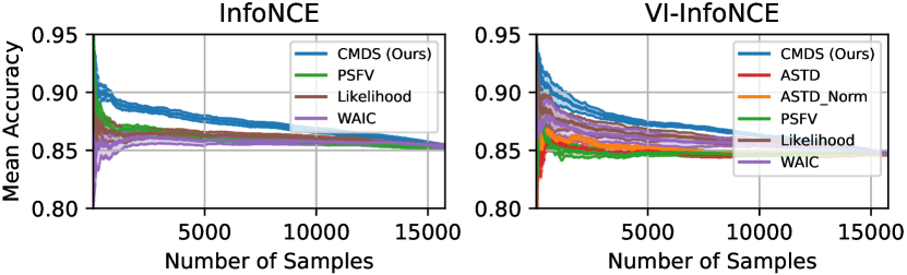
Figure 3: (Left) Retention Curves on Pubmed for a InfoNCE model. (Right) Retention Curves on Pubmed for VI-InfoNCE.

fig:ret_curves_cora_models

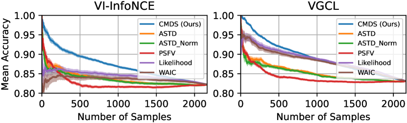
Figure 4: (Left) Retention Curves on Cora for VI-InfoNCE. (Right) Retention Curves on Cora for VGCL.

fig:ret_curves_citeseer_models

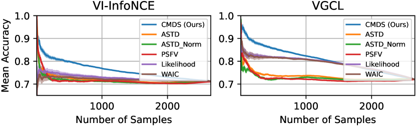
Figure 5: (Left) Retention Curves on CiteSeer for VI-InfoNCE. (Right) Retention Curves on CiteSeer for VGCL.

fig:vi_inf_heatmap

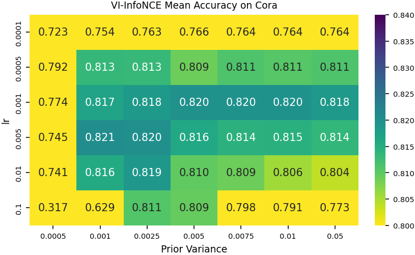
Figure 6: Heatmap over the parameters of a VI-InfoNCE model on Cora

fig:paramsnetwork

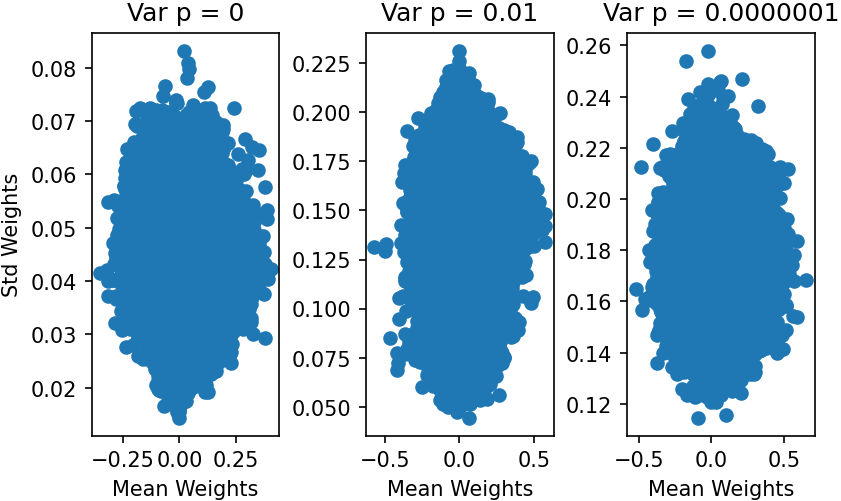
Figure 7: Weight parameters in the first layer of VGCL under different regularizations of the variance of the variational family. The stronger the influence of the hyperprior, the larger the standard deviation of the weight distributions.

Appendix G Related Work

Uncertainty in Contrastive Learning

Existing works on uncertainty in contrastive learning generally focus on measuring embedding uncertainty. They do this by using the trained encoder to map the data point in question into the embedding space and then considering different measures of uncertainty. Ardeshir and Azizan (2022) measure the variance of the embeddings under different augmentations and Hasanzadeh et al. (2021) additionally consider the uncertainty in the weights of the encoder. The latter then use the average standard deviation (ASTD) of the features of the embeddings. Sometimes, surrogate distributions such as the one obtained from a Gaussian Mixture Model on the embeddings are used to obtain a probability density that can be reasoned about (Ardeshir and Azizan, 2022; Wu and Goodman, 2020). Other papers try to approximate a notion of hardness of examples by changing a scalar in the similarity function (the temperature) based on intuition and empirical observations (Zhang et al., 2021). Note that, Hasanzadeh et al. (2021) and Sharma et al. (2023) also perform Bayesian inference in a contrastive learning setting. The former use this to improve the network performance by learning the parameters of the augmentations and do not learn the weights in the projection head. They use Beta-Bernoulli priors and propose to measure the uncertainty in the embedding space using the ASTD. In contrast to that, we propose to measure uncertainty with regard to the likelihood of the probabilistic model and propose the CMDS. We use the ASTD as a baseline in our experiments and outperform it by a large margin. Furthermore, our improvements in performance in accuracy are not due to improved augmentations, but due to a better specification of the variational family. The latter do not consider learning on graphs and they also only perform Bayesian inference over the last layer of the network, as opposed to the full-network inference in our work.

Bayesian neural networks

Bayesian neural networks promise to marry the expressivity of neural networks with the principled statistical properties of Bayesian inference (MacKay, 1992; Neal, 1993). However, approximate inference in these complex models has remained challenging (Jospin et al., 2022). Approximate inference techniques lie on a spectrum of quality and computational cost, from cheap local approximations like Laplace inference (Laplace, 1774; MacKay, 1992; Khan et al., 2019; Daxberger et al., 2021), stochastic weight averaging (Izmailov et al., 2018; Maddox et al., 2019), and dropout (Gal and Ghahramani, 2016; Kingma et al., 2015), via variational approximations with different levels of complexity (e.g., Graves, 2011; Blundell et al., 2015; Louizos and Welling, 2016; Khan et al., 2018; Osawa et al., 2019), across ensemble-based methods (Lakshminarayanan et al., 2017; Wang et al., 2019; Wilson and Izmailov, 2020; Ciosek et al., 2020; He et al., 2020a; D’Angelo et al., 2021; D’Angelo and Fortuin, 2021), up to the very expensive but asymptotically correct Markov Chain Monte Carlo (MCMC) approaches (e.g., Neal, 1993; Neal et al., 2011; Welling and Teh, 2011; Garriga-Alonso and Fortuin, 2021; Izmailov et al., 2021). Apart from the challenges relating to approximate inference, recent work has also studied the question of prior choice for BNNs (e.g., Fortuin et al., 2021, 2022; Nabarro et al., 2022; Sharma et al., 2023; Fortuin, 2022, and references therein) and how to perform model selection in this framework (e.g., Immer et al., 2021, 2022; Rothfuss et al., 2021, 2022; van der Ouderaa and van der Wilk, 2022; Schwöbel et al., 2022). In our work, we apply these methods to the graph contrastive learning setting, which to the best of our knowledge has not been studied with full-network variational inference before (see also discussion above).

Graph Contrastive Learning

In recent years, methods that facilitate learning on graphs have made rapid progress and have been applied to a large variety of problem settings (e.g., Kipf and Welling, 2016; Xu et al., 2018; Isufi and Mazzola, 2021; Isufi et al., 2022). Graph contrastive learning (GCL) applies these advances to unlabeled data by using positive and negative examples. Hereby, the contrastive loss is typically based on the InfoNCE (InfoMax) principle, which aims to maximize the mutual information between the input data and its corresponding latent representation (You et al., 2020; Oord et al., 2018; Zhu et al., 2020). Most existing research focuses on improving the performance of GCL by designing methods that produce better augmentations (e.g., Hassani and Khasahmadi, 2020; Lin et al., 2023; Liu et al., 2022), improve negative sampling (e.g., Xia et al., 2022; Robinson et al., 2021; Zhu et al., 2020) or change the loss function (e.g., Peng et al., 2020; Lin et al., 2023). In contrast to that, the improvements in accuracy in our work stem from introducing a distribution over the weights.

References

- Aitchison and Ganev (2023) Laurence Aitchison and Stoil Ganev. Infonce is a variational autoencoder. ArXiv, abs/2107.02495, 2023.
- Ardeshir and Azizan (2022) Shervin Ardeshir and Navid Azizan. Embedding reliability: On the predictability of downstream performance. In NeurIPS ML Safety Workshop, 2022. URL https://openreview.net/forum?id=TedqYedIERd.
- Blundell et al. (2015) Charles Blundell, Julien Cornebise, Koray Kavukcuoglu, and Daan Wierstra. Weight uncertainty in neural networks. In ICML, 2015.
- Chen et al. (2020) Ting Chen, Simon Kornblith, Mohammad Norouzi, and Geoffrey Hinton. A simple framework for contrastive learning of visual representations. In Hal Daumé III and Aarti Singh, editors, Proceedings of the 37th International Conference on Machine Learning, volume 119 of Proceedings of Machine Learning Research, pages 1597–1607. PMLR, 13–18 Jul 2020. URL https://proceedings.mlr.press/v119/chen20j.html.
- Ciosek et al. (2020) Kamil Ciosek, Vincent Fortuin, Ryota Tomioka, Katja Hofmann, and Richard Turner. Conservative uncertainty estimation by fitting prior networks. In International Conference on Learning Representations, 2020.
- D’Angelo and Fortuin (2021) Francesco D’Angelo and Vincent Fortuin. Repulsive deep ensembles are bayesian. Advances in Neural Information Processing Systems, 34:3451–3465, 2021.
- D’Angelo et al. (2021) Francesco D’Angelo, Vincent Fortuin, and Florian Wenzel. On stein variational neural network ensembles. arXiv preprint arXiv:2106.10760, 2021.
- Daxberger et al. (2021) Erik Daxberger, Agustinus Kristiadi, Alexander Immer, Runa Eschenhagen, Matthias Bauer, and Philipp Hennig. Laplace redux–effortless Bayesian deep learning. In NeurIPS, 2021.
- Daxberger and Hernández-Lobato (2019) Erik A. Daxberger and José Miguel Hernández-Lobato. Bayesian variational autoencoders for unsupervised out-of-distribution detection. CoRR, abs/1912.05651, 2019. URL http://arxiv.org/abs/1912.05651.
- Fortuin (2022) Vincent Fortuin. Priors in bayesian deep learning: A review. International Statistical Review, 90(3):563–591, 2022.
- Fortuin et al. (2021) Vincent Fortuin, Adrià Garriga-Alonso, Mark van der Wilk, and Laurence Aitchison. Bnnpriors: A library for bayesian neural network inference with different prior distributions. Software Impacts, 9:100079, 2021.
- Fortuin et al. (2022) Vincent Fortuin, Adrià Garriga-Alonso, Sebastian W Ober, Florian Wenzel, Gunnar Ratsch, Richard E Turner, Mark van der Wilk, and Laurence Aitchison. Bayesian neural network priors revisited. In International Conference on Learning Representations, 2022.
- Gal and Ghahramani (2016) Yarin Gal and Zoubin Ghahramani. Dropout as a Bayesian approximation: Representing model uncertainty in deep learning. In ICML, 2016.
- Gama et al. (2020) Fernando Gama, Elvin Isufi, Geert Leus, and Alejandro Ribeiro. Graphs, convolutions, and neural networks: From graph filters to graph neural networks. IEEE Signal Processing Magazine, 37(6):128–138, 2020.
- Garriga-Alonso and Fortuin (2021) Adrià Garriga-Alonso and Vincent Fortuin. Exact Langevin dynamics with stochastic gradients. arXiv preprint arXiv:2102.01691, 2021.
- Graves (2011) Alex Graves. Practical variational inference for neural networks. In NIPS, 2011.
- Hasanzadeh et al. (2021) Arman Hasanzadeh, Mohammadreza Armandpour, Ehsan Hajiramezanali, Mingyuan Zhou, Nick Duffield, and Krishna Narayanan. Bayesian graph contrastive learning. CoRR, abs/2112.07823, 2021. URL https://arxiv.org/abs/2112.07823.
- Hassani and Khasahmadi (2020) Kaveh Hassani and Amir Hosein Khasahmadi. Contrastive multi-view representation learning on graphs. In International conference on machine learning, pages 4116–4126. PMLR, 2020.
- He et al. (2020a) Bobby He, Balaji Lakshminarayanan, and Yee Whye Teh. Bayesian deep ensembles via the neural tangent kernel. Advances in neural information processing systems, 33:1010–1022, 2020a.
- He et al. (2020b) Kaiming He, Haoqi Fan, Yuxin Wu, Saining Xie, and Ross Girshick. Momentum contrast for unsupervised visual representation learning. In Proceedings of the IEEE/CVF conference on computer vision and pattern recognition, pages 9729–9738, 2020b.
- Immer et al. (2021) Alexander Immer, Matthias Bauer, Vincent Fortuin, Gunnar Rätsch, and Mohammad Emtiyaz Khan. Scalable marginal likelihood estimation for model selection in deep learning. In ICML, 2021.
- Immer et al. (2022) Alexander Immer, Tycho FA van der Ouderaa, Vincent Fortuin, Gunnar Rätsch, and Mark van der Wilk. Invariance learning in deep neural networks with differentiable Laplace approximations. In NeurIPS, 2022.
- Isufi and Mazzola (2021) Elvin Isufi and Gabriele Mazzola. Graph-time convolutional neural networks. In 2021 IEEE Data Science and Learning Workshop (DSLW), pages 1–6, 2021. 10.1109/DSLW51110.2021.9523412.
- Isufi et al. (2022) Elvin Isufi, Fernando Gama, and Alejandro Ribeiro. Edgenets: Edge varying graph neural networks. IEEE Transactions on Pattern Analysis and Machine Intelligence, 44(11):7457–7473, 2022. 10.1109/TPAMI.2021.3111054.
- Izmailov et al. (2018) Pavel Izmailov, Dmitrii Podoprikhin, Timur Garipov, Dmitry Vetrov, and Andrew Gordon Wilson. Averaging weights leads to wider optima and better generalization. In 34th Conference on Uncertainty in Artificial Intelligence 2018, UAI 2018, pages 876–885, 2018.
- Izmailov et al. (2021) Pavel Izmailov, Sharad Vikram, Matthew D Hoffman, and Andrew Gordon Wilson. What are Bayesian neural network posteriors really like? In ICML, 2021.
- Jospin et al. (2022) Laurent Valentin Jospin, Hamid Laga, Farid Boussaid, Wray Buntine, and Mohammed Bennamoun. Hands-on bayesian neural networks - a tutorial for deep learning users. IEEE Computational Intelligence Magazine, 17(2):29–48, 2022.
- Khan et al. (2018) Mohammad Khan, Didrik Nielsen, Voot Tangkaratt, Wu Lin, Yarin Gal, and Akash Srivastava. Fast and scalable Bayesian deep learning by weight-perturbation in Adam. In ICML, 2018.
- Khan et al. (2019) Mohammad Emtiyaz E Khan, Alexander Immer, Ehsan Abedi, and Maciej Korzepa. Approximate inference turns deep networks into Gaussian processes. In NeurIPS, 2019.
- Kingma and Ba (2014) Diederik Kingma and Jimmy Ba. Adam: A method for stochastic optimization. International Conference on Learning Representations, 12 2014.
- Kingma et al. (2015) Diederik P Kingma, Tim Salimans, and Max Welling. Variational dropout and the local reparameterization trick. In Advances in Neural Information Processing Systems 28, 2015.
- Kipf and Welling (2016) Thomas N Kipf and Max Welling. Semi-supervised classification with graph convolutional networks. arXiv preprint arXiv:1609.02907, 2016.
- Lakshminarayanan et al. (2017) Balaji Lakshminarayanan, Alexander Pritzel, and Charles Blundell. Simple and scalable predictive uncertainty estimation using deep ensembles. In NIPS, 2017.
- Laplace (1774) Pierre-Simon Laplace. Mémoires de mathématique et de physique, tome sixieme. 1774.
- Li et al. (2021) Yazhe Li, Roman Pogodin, Danica J Sutherland, and Arthur Gretton. Self-supervised learning with kernel dependence maximization. Advances in Neural Information Processing Systems, 34:15543–15556, 2021.
- Lin et al. (2023) Lu Lin, Jinghui Chen, and Hongning Wang. Spectral augmentation for self-supervised learning on graphs. In The Eleventh International Conference on Learning Representations, 2023. URL https://openreview.net/forum?id=DjzBCrMBJ_p.
- Liu et al. (2022) Nian Liu, Xiao Wang, Deyu Bo, Chuan Shi, and Jian Pei. Revisiting graph contrastive learning from the perspective of graph spectrum. In Alice H. Oh, Alekh Agarwal, Danielle Belgrave, and Kyunghyun Cho, editors, Advances in Neural Information Processing Systems, 2022. URL https://openreview.net/forum?id=L0U7TUWRt_X.
- Louizos and Welling (2016) Christos Louizos and Max Welling. Structured and efficient variational deep learning with matrix Gaussian posteriors. In ICML, 2016.
- MacKay (1992) David JC MacKay. A practical Bayesian framework for backpropagation networks. Neural Computation, 4(3), 1992.
- Maddox et al. (2019) Wesley J Maddox, Pavel Izmailov, Timur Garipov, Dmitry P Vetrov, and Andrew Gordon Wilson. A simple baseline for Bayesian uncertainty in deep learning. In NeurIPS, 2019.
- Nabarro et al. (2022) Seth Nabarro, Stoil Ganev, Adrià Garriga-Alonso, Vincent Fortuin, Mark van der Wilk, and Laurence Aitchison. Data augmentation in bayesian neural networks and the cold posterior effect. In Uncertainty in Artificial Intelligence, pages 1434–1444. PMLR, 2022.
- Neal (1993) Radford M Neal. Bayesian learning via stochastic dynamics. In Advances in neural information processing systems, pages 475–482, 1993.
- Neal et al. (2011) Radford M Neal et al. MCMC using Hamiltonian dynamics. Handbook of Markov Chain Monte Carlo, 2(11), 2011.
- Oord et al. (2018) Aaron van den Oord, Yazhe Li, and Oriol Vinyals. Representation learning with contrastive predictive coding. arXiv preprint arXiv:1807.03748, 2018.
- Osawa et al. (2019) Kazuki Osawa, Siddharth Swaroop, Mohammad Emtiyaz E Khan, Anirudh Jain, Runa Eschenhagen, Richard E Turner, and Rio Yokota. Practical deep learning with Bayesian principles. In NeurIPS, 2019.
- Peng et al. (2020) Zhen Peng, Wenbing Huang, Minnan Luo, Qinghua Zheng, Yu Rong, Tingyang Xu, and Junzhou Huang. Graph representation learning via graphical mutual information maximization. In Proceedings of The Web Conference 2020, pages 259–270, 2020.
- Robinson et al. (2021) Joshua David Robinson, Ching-Yao Chuang, Suvrit Sra, and Stefanie Jegelka. Contrastive learning with hard negative samples. In International Conference on Learning Representations, 2021. URL https://openreview.net/forum?id=CR1XOQ0UTh-.
- Rothfuss et al. (2021) Jonas Rothfuss, Vincent Fortuin, Martin Josifoski, and Andreas Krause. Pacoh: Bayes-optimal meta-learning with pac-guarantees. In International Conference on Machine Learning, pages 9116–9126. PMLR, 2021.
- Rothfuss et al. (2022) Jonas Rothfuss, Martin Josifoski, Vincent Fortuin, and Andreas Krause. Pac-bayesian meta-learning: From theory to practice. arXiv preprint arXiv:2211.07206, 2022.
- Sanchez-Fernandez et al. (2022) Ana Sanchez-Fernandez, Elisabeth Rumetshofer, Sepp Hochreiter, and Günter Klambauer. Contrastive learning of image- and structure-based representations in drug discovery. In ICLR2022 Machine Learning for Drug Discovery, 2022. URL https://openreview.net/forum?id=OdXKRtg1OG.
- Schwöbel et al. (2022) Pola Schwöbel, Martin Jørgensen, Sebastian W Ober, and Mark Van Der Wilk. Last layer marginal likelihood for invariance learning. In International Conference on Artificial Intelligence and Statistics, pages 3542–3555. PMLR, 2022.
- Sen et al. (2008) Prithviraj Sen, Galileo Namata, Mustafa Bilgic, Lise Getoor, Brian Gallagher, and Tina Eliassi-Rad. Collective classification in network data articles. AI Magazine, 29:93–106, 09 2008. 10.1609/aimag.v29i3.2157.
- Sharma et al. (2023) Mrinank Sharma, Tom Rainforth, Yee Whye Teh, and Vincent Fortuin. Incorporating unlabelled data into bayesian neural networks. arXiv preprint arXiv:2304.01762, 2023.
- Ustyuzhaninov et al. (2020) Ivan Ustyuzhaninov, Ieva Kazlauskaite, Markus Kaiser, Erik Bodin, Neill Campbell, and Carl Henrik Ek. Compositional uncertainty in deep gaussian processes. In Jonas Peters and David Sontag, editors, Proceedings of the 36th Conference on Uncertainty in Artificial Intelligence (UAI), volume 124 of Proceedings of Machine Learning Research, pages 480–489. PMLR, 03–06 Aug 2020. URL https://proceedings.mlr.press/v124/ustyuzhaninov20a.html.
- van der Ouderaa and van der Wilk (2022) Tycho FA van der Ouderaa and Mark van der Wilk. Learning invariant weights in neural networks. In Uncertainty in Artificial Intelligence, pages 1992–2001. PMLR, 2022.
- Veličković et al. (2019) Petar Veličković, William Fedus, William L. Hamilton, Pietro Liò, Yoshua Bengio, and R Devon Hjelm. Deep graph infomax. In International Conference on Learning Representations, 2019. URL https://openreview.net/forum?id=rklz9iAcKQ.
- Wang and Isola (2020) Tongzhou Wang and Phillip Isola. Understanding contrastive representation learning through alignment and uniformity on the hypersphere. In International Conference on Machine Learning, pages 9929–9939. PMLR, 2020.
- Wang et al. (2019) Ziyu Wang, Tongzheng Ren, Jun Zhu, and Bo Zhang. Function space particle optimization for bayesian neural networks. In International Conference on Learning Representations, 2019.
- Welling and Teh (2011) Max Welling and Yee W Teh. Bayesian learning via stochastic gradient langevin dynamics. In ICML, 2011.
- Wilson and Izmailov (2020) Andrew Gordon Wilson and Pavel Izmailov. Bayesian deep learning and a probabilistic perspective of generalization. In NeurIPS, 2020.
- Wu and Goodman (2020) Mike Wu and Noah Goodman. A simple framework for uncertainty in contrastive learning. arXiv preprint arXiv:2010.02038, 2020.
- Wu et al. (2020) Zonghan Wu, Shirui Pan, Fengwen Chen, Guodong Long, Chengqi Zhang, and S Yu Philip. A comprehensive survey on graph neural networks. IEEE transactions on neural networks and learning systems, 32(1):4–24, 2020.
- Xia et al. (2022) Jun Xia, Lirong Wu, Ge Wang, and Stan Z. Li. Progcl: Rethinking hard negative mining in graph contrastive learning. In International conference on machine learning. PMLR, 2022.
- Xie et al. (2021) Enze Xie, Jian Ding, Wenhai Wang, Xiaohang Zhan, Hang Xu, Peize Sun, Zhenguo Li, and Ping Luo. Detco: Unsupervised contrastive learning for object detection. In 2021 IEEE/CVF International Conference on Computer Vision (ICCV), pages 8372–8381, 2021. 10.1109/ICCV48922.2021.00828.
- Xu et al. (2018) Keyulu Xu, Weihua Hu, Jure Leskovec, and Stefanie Jegelka. How powerful are graph neural networks? arXiv preprint arXiv:1810.00826, 2018.
- Yang et al. (2016) Zhilin Yang, William Cohen, and Ruslan Salakhudinov. Revisiting semi-supervised learning with graph embeddings. In International conference on machine learning, pages 40–48. PMLR, 2016.
- You et al. (2020) Yuning You, Tianlong Chen, Yongduo Sui, Ting Chen, Zhangyang Wang, and Yang Shen. Graph contrastive learning with augmentations. In H. Larochelle, M. Ranzato, R. Hadsell, M.F. Balcan, and H. Lin, editors, Advances in Neural Information Processing Systems, volume 33, pages 5812–5823. Curran Associates, Inc., 2020. URL https://proceedings.neurips.cc/paper_files/paper/2020/file/3fe230348e9a12c13120749e3f9fa4cd-Paper.pdf.
- Zhang et al. (2021) Oliver Zhang, Mike Wu, Jasmine Bayrooti, and Noah Goodman. Temperature as uncertainty in contrastive learning, 2021.
- Zhao et al. (2018) Shengjia Zhao, Jiaming Song, and Stefano Ermon. The information autoencoding family: A lagrangian perspective on latent variable generative models, 2018.
- Zhu et al. (2020) Yanqiao Zhu, Yichen Xu, Feng Yu, Qiang Liu, Shu Wu, and Liang Wang. Deep Graph Contrastive Representation Learning. In ICML Workshop on Graph Representation Learning and Beyond, 2020. URL http://arxiv.org/abs/2006.04131.
- Zhu et al. (2021) Yanqiao Zhu, Yichen Xu, Qiang Liu, and Shu Wu. An empirical study of graph contrastive learning. In Thirty-fifth Conference on Neural Information Processing Systems Datasets and Benchmarks Track (Round 2), 2021. URL https://openreview.net/forum?id=UuUbIYnHKO.