Eliminating confounder-induced bias
in the statistics of intervention

Orestis Loukas,  Ho Ryun Chung

Institute for Medical Bioinformatics and Biostatistics
Philipps-Universität Marburg
Hans-Meerwein-Straße 6, 35032 Germany

Abstract

Experimental and observational studies often lead to spurious association between the outcome and independent variables describing the intervention, because of confounding to third-party factors. Even in randomized clinical trials, confounding might be unavoidable due to small sample sizes. Practically, this poses a problem, because it is either expensive to re-design and conduct a new study or even impossible to alleviate the contribution of some confounders due to e.g. ethical concerns. Here, we propose a method to consistently derive hypothetical studies that retain as many of the dependencies in the original study as mathematically possible, while removing any association of observed confounders to the independent variables. Using historic studies, we illustrate how the confounding-free scenario re-estimates the effect size of the intervention. The new effect size estimate represents a concise prediction in the hypothetical scenario which paves a way from the original data towards the design of future studies.

1 Introduction

A large part of quantitative literature [1, 2, 3, 4] in fields ranging from biometrics and clinical studies to sociology and psychometrics is concerned with determining an effect size estimate to quantify the association of some controlling condition(s) to the outcome of interest. Such estimate is usually an $Odds$ ratio ($OR$), relative risk ($RR$) or absolute risk reduction ($ARR$). Ideally, the computed effect size estimate must offer understanding into the direct causal relationship of the response to an exposure or intervention in the population. This insight is essential for meaningful inference from the data.

However, various external factors could bias a “naive” inference from the study. Consequently, the estimation of effect size or its direction (e.g. risk reduction vs. enhancement) might more reflect some underlying systematic asymmetry in the study population than the targeted relationship between intervention/exposure and outcome. Conceptualizing the extend of the problem is challenging, as it depends on the chosen theoretical framework and modeling tools used in the statistical analysis. The aim of this work is not to offer an overview of the various theoretical and methodological challenges, as e.g. discussed in [5, 6, 7]. Instead, utilizing a unified framework [8] rooted in information theory, we furnish formal tools to eradicate any detected confounding (whether randomly induced or systematic) from the data.

Commonly, clinical trials and observational studies investigate an outcome $y$ represented by a variable $Y$ which could be either categorical like success  of  treatment or metric like blood  pressure. This variable responds to an intervention which comprises the change of some specified conditions summarized by the levels $\boldsymbol{x}$ of $m$ independent variables $\boldsymbol{X}$ like treatment  group, diagnostic  tool, geographic location etc. Evidently, $n$ additional variables $\boldsymbol{S}$ that summarize the demographic, anthropometric or clinical profile $\boldsymbol{s}$ of studied subjects can influence the outcome $y$. Sometimes such factors are under our control and sometimes not. As long as we are not directly interested in the association of $Y$ and $\boldsymbol{X}$ to $\boldsymbol{S}$, we can designate latter variables as (suspected) confounders and refer to their influence on the effect size estimate of the intervention as bias.

The situation resulting from the existence of confounders, which interact with both the outcome $y$ and the examined groups $\boldsymbol{x}$, is succinctly illustrated in undirected graph 1.

Figure 1: Undirected three-way graph depicting two-factor associations in the original study.

In addition, higher-order dependencies might simultaneously associate all factors leading to non-trivial three-way effects that cannot be predicted just by the drawn edges (hence requiring a hypergraph to depict). From contingency tables of the study at hand, the statistical analysis of such graphs on dependencies aims at inferring an idea about causal associations. Besides asserting a meaningful temporal association (“the cause precedes the outcome”), there is a long way to go to prove causality in the intervention [9], as there might always exist additional confounders that are entirely omitted from the data or when recorded confounders act as a proxy of the actual causal ones. In the following, we concentrate on those attributes $Y$, $\boldsymbol{X}$ and $\boldsymbol{S}$ only, that are explicitly recorded in the study to investigate their associations.

A first step towards counteracting the adverse effect of confounders which bias statistical analysis perplexing causal inference is the – often rhetorical – question:

How would the effect of the intervention on the outcome look like in a hypothetical scenario

where the independent variables would not depend on observed confounders? (1)

There are many reasons to target the particular association of $\boldsymbol{X}$ to $\boldsymbol{S}$ in the three-way graph. At the operational level, structural differences in the distribution of confounders among intervention groups can be manipulated [10] during the design of future experimental and clinical studies. For example, one can decide how many smokers  with  asthma would be included in each treatment group.

Removing the association between $\boldsymbol{X}$ and $\boldsymbol{S}$ balances the generically disparate distribution of confounders over intervention groups $\boldsymbol{x}$, hence restoring a symmetry [11] to enable “fair” comparisons among groups. We call this symmetry structural parity. Asymptotically given an infinite pool of study subjects, such structural parity must be exactly realized to manifest the essence of a truly randomized study, at least as far as designated confounders are concerned. Conversely, the expected $\boldsymbol{X}-\boldsymbol{S}$ association in a finite study must reflect structural parity, when the expectation is computed over infinitely many properly randomized trials with finite number of participants each.

In addition to conceptual arguments which favor the hypothesis about structural parity, a cautionary aspect supports targeting this association only: Arbitrarily modifying the influence of $\boldsymbol{S}$ on $Y$ could disrupt the inherent characteristics of confounders. Generally, we wish to avoid hypothesizing larger modifications that could invalidate biological and physical laws which underlie the associations, unless there is a clear understanding about the association map of $\boldsymbol{S}$ to $Y$ and $\boldsymbol{X}$ through external sources. Knowledge transfer is certainly an interesting and fruitful path to explore. For concreteness nevertheless, we henceforth concentrate on the knowledge transmitted by one study individually.

In the present work, we explain how a well-known information-theoretic method can precisely answer the hypothetical question 1 by uniquely producing an alternative expectation about the three-way graph 1. In this alternative scenario, we just remove one association in a targeted way, while ensuring that all other dependencies (including three-factor effects) are left as intact as mathematically possible. Without relying on special asymptotic distributions and simplifying assumptions such as equal number of participants in each group or low incidence rates, this top-down approach offers a unique answer to the confounding-free scenario regarding the dependency of $Y$ on $\boldsymbol{X}$ that quantifies intervention effects. Through various historic paradigms, we exemplify the ability of the suggested methodology to give a definite answer to hypothetical scenario 1 in versatile settings.

2 Methods

After collecting $N$ microdata entries over a study, we can describe any subject by specifying the three attributes $y$, $\boldsymbol{x}$ and $\boldsymbol{s}$ from some domains $\mathcal{D}_{Y}$, $\mathcal{D}_{\boldsymbol{X}}$ and $\mathcal{D}_{\boldsymbol{S}}$ respectively. In that way, the three-way contingency table can be succinctly provided through the empirical joint distribution $\mathfrak{f}\equiv\mathfrak{f}_{Y,\boldsymbol{X},\boldsymbol{S}}$ whose probabilities are given by the relative frequencies $f(y,\boldsymbol{x},\boldsymbol{s})$ in the dataset. In the following, we reserve letter $\mathfrak{f}$ for the empirical statistics of the original study. Usually, the derived statistics of a study express our expectation about correlations and associations in the population. In principle, our expectation for each entry in the three-way contingency table does not need to adhere to $\mathfrak{f}$, even if some statistics such as the incidence rate $f_{Y}(y)$, i.e. the prevalence of outcome $y$ are empirically inferred from the given study.

Essentially, the conductor of the analysis is interested in the interventional influence of independent variables on the outcome, which is represented in the original data by the rate of each outcome $y$ given level $\boldsymbol{x}$ as a conditional relative frequency

$$f_{Y|\boldsymbol{X}}(y|\boldsymbol{x})=\frac{f_{Y,\boldsymbol{X}}(y,\boldsymbol{x})}{f_{\boldsymbol{X}}(\boldsymbol{x})}\quad\text{for}\quad y\in\mathcal{D}_{Y}\quad\text{and}\quad\boldsymbol{x}\in\mathcal{D}_{\boldsymbol{X}}~{}.$$ (2)

Whenever the additional variables $\boldsymbol{S}$ become substantially associated to the independent variables $\boldsymbol{X}$, there might be undesired confounding. Such non-trivial association between confounders and intervention variables is reflected on the structural difference in the distribution of confounder profiles $\boldsymbol{s}$ between the different groups $\boldsymbol{x}$ quantified by conditional distribution $\mathfrak{f}_{\boldsymbol{S}|\boldsymbol{X}}$ with

$$f_{\boldsymbol{S}|\boldsymbol{X}}(\boldsymbol{s}|\boldsymbol{x})=\frac{f_{\boldsymbol{X},\boldsymbol{S}}(\boldsymbol{x},\boldsymbol{s})}{f_{\boldsymbol{X}}(\boldsymbol{x})}\quad\text{for}\quad\boldsymbol{x}\in\mathcal{D}_{\boldsymbol{X}}\quad\text{and}\quad\boldsymbol{s}\in\mathcal{D}_{\boldsymbol{S}}~{},$$ (3)

which will not be generically independent of group $\boldsymbol{x}$. Eq. (3) measures structural heterogeneity [12, 13] in the clinical trial or case-control study; potentially also in the target population.

More generally, a joint distribution $\mathfrak{p}$ of $Y$ with $\boldsymbol{X}$ and $\boldsymbol{S}$ suffices to unambiguously characterize all possible associations regarding the attributes like structural differences and confounding effects. In particular, any marginal distribution like prevalences $\mathfrak{p}_{Y}$, $\mathfrak{p}_{\boldsymbol{X}}$ and $\mathfrak{p}_{\boldsymbol{S}}$ can be calculated from the joint distribution of the study. Furthermore, conditional distributions like $\mathfrak{p}_{Y|X}$ are estimated as ratios of marginals $p_{Y|\boldsymbol{X}}(y|\boldsymbol{x})=p_{Y,\boldsymbol{X}}(y,\boldsymbol{x})/p_{\boldsymbol{X}}(\boldsymbol{x})$ from the joint distribution. Given the conditional distribution any odds and risk metric can be inferred. For our purposes, the domain of attributes over $\mathbb{F}=\mathbb{N},\mathbb{Z},\mathbb{Q},\{\texttt{true},\texttt{false}\},\dots$ can be empirically determined by

$$\mathcal{D}_{Y}=\{y\in\mathbb{F}|f_{Y}(y)>0\}\quad,\quad\mathcal{D}_{\boldsymbol{X}}=\{\boldsymbol{x}\in\mathbb{F}^{m}|f_{\boldsymbol{X}}(\boldsymbol{x})>0\}\quad\text{and}\quad\mathcal{D}_{\boldsymbol{S}}=\{\boldsymbol{s}\in\mathbb{F}^{n}|f_{\boldsymbol{S}}(\boldsymbol{s})>0\}~{},$$ (4)

so that any distribution $\mathfrak{p}$ we are going to consider is defined on the simplex over $\mathcal{D}=\mathcal{D}_{Y}\times\mathcal{D}_{\boldsymbol{X}}\times\mathcal{D}_{\boldsymbol{S}}$. Automatically, this excludes any unobserved profiles $\boldsymbol{s}$ or non-realized intervention groups $\boldsymbol{x}$.

Given a distribution $\mathfrak{p}$ we can sample counts for all elements in the Cartesian product $\mathcal{D}$. In other words, we sample contingency tables, i.e. studies, that – in expectation – reproduce the statistics of $\mathfrak{p}$. In the context of removing confounding effects, any hypothetical scenario is required to:

1. be self-consistent w.r.t. investigated variables $Y,\boldsymbol{X}$ and $\boldsymbol{S}$, i.e. unequivocally prescribe counts for each cell in the three-way contingency table with all entries summing to $N$

2. respect the observed lower-order marginals

3. be confounding-free (at least regarding all designated observed confounders), i.e. $\mathfrak{p}_{\boldsymbol{S}|\boldsymbol{X}}=\mathfrak{f}_{\boldsymbol{S}}$

4. otherwise, stay as close as possible to the original statistics of $\mathfrak{f}$

The presence of some distribution on the simplex over $\mathcal{D}$ asserted by point 1 is epistemologically needed in order to be able to discuss the remaining points 2, 3 and 4. In that way, the requirement of self-consistency automatically excludes methods like the pooled estimator of the Mantel-Haenszel formula [14] that are rooted in heuristics and special (realistically mostly unfulfilled) limits failing to unambiguously provide a concise estimate for the expectation of the hypothetical contingency table. As always in statistics, each alternative study on its own does not need to satisfy the last three requirements. Points 2-4 must become asymptotically fulfilled, when $N\rightarrow\infty$ or by taking the expectation over infinitely many studies at fixed $N$ that are generated from $\mathfrak{p}$. Due to its epistemological importance for the hypothetical study, we refer to $\mathfrak{p}$ as the fictitious-study distribution, whose $Y-\boldsymbol{X}$ marginal distribution logically implies

$$Odds_{\mathfrak{p}}(\texttt{event}|\boldsymbol{x})=\frac{\mathfrak{p}_{Y|\boldsymbol{X}}(\texttt{event}|\boldsymbol{x})}{1-\mathfrak{p}_{Y|\boldsymbol{X}}(\texttt{event}|\boldsymbol{x})}~{},$$ (5)

leading w.r.t. control reference $\boldsymbol{x}_{0}\in\mathcal{D}_{\boldsymbol{X}}$ to the

$$Intervention_{\mathfrak{p}}=\frac{Odds_{\mathfrak{p}}(\texttt{event}|\,\,\boldsymbol{x}\,)}{Odds_{\mathfrak{p}}(\texttt{event}|\boldsymbol{x}_{0})}\quad\text{for}\quad\boldsymbol{x}\in\mathcal{D}_{\boldsymbol{X}},$$ (6)

as a measure of the effect size in a binary study $\mathcal{D}_{Y}=\{\texttt{event},\texttt{no\,\,event}\}$. Accordingly, sensible three-factor dependencies can be quantified by

$$OR=\frac{Odds_{\mathfrak{p}}(\texttt{event}|\boldsymbol{x},\boldsymbol{s})}{Odds_{\mathfrak{p}}(\texttt{event}|\boldsymbol{x}_{0},\boldsymbol{s})}$$ (7)

where

$$Odds_{\mathfrak{p}}(\texttt{event}|\boldsymbol{x},\boldsymbol{s})=\frac{\mathfrak{p}_{Y|\boldsymbol{X},\boldsymbol{S}}(\texttt{event}|\boldsymbol{x},\boldsymbol{s})}{1-\mathfrak{p}_{Y|\boldsymbol{X},\boldsymbol{S}}(\texttt{event}|\boldsymbol{x},\boldsymbol{s})}~{}.$$ (8)

The distribution of logistic regression which is often employed [15, 16] in this context fails to fulfill point 3, since it does not remove structural disparity in the graph 1, as we show using the concrete example in Section 3.2. To proceed further we therefore need to employ new tools that we choose from information theory and specifically the framework of total empiricism (TotEm [17]).

2.1 Minimization of information divergence given hypothetical scenario

Even if we do not wish to fully adhere to the empirical statistics of $\mathfrak{f}$, we want any hypothetical study to at least partially resemble the statistical properties of the original study, as advocated by point 4. In the spirit of mitigating discriminatory bias [8], the notion of remaining “close” to the original contingency table can be covariantly (i.e. in a model-agnostic way) realized as an optimization problem from information theory. Specifically, we propose constructing a joint distribution $\mathfrak{p}$ as close as possible to the original $\mathfrak{f}$ that satisfies

$$\text{structural {p}arity:}\quad\mathfrak{p}_{\boldsymbol{X},\boldsymbol{S}}\overset{!}{=}\mathfrak{f}_{\boldsymbol{X}}\cdot\mathfrak{f}_{\boldsymbol{S}}\quad\text{and}\quad\text{confounder {r}ealism}\quad\mathfrak{p}_{Y,\boldsymbol{S}}\overset{!}{=}\mathfrak{f}_{Y,\boldsymbol{S}}~{}.$$ (9)

By parity and realism, we exclusively refer to associations between observed attributes provided in the original contingency table. Therefore, the present information-theoretic framework is not going to make statements about unobserved confounders [18, 19]. As a working assumption of this paper, we further entertain that the observed influence of the confounders on the outcome – quantified by marginal $\mathfrak{f}_{Y,\boldsymbol{S}}$ – fairly depicts reality, at least within the scope of the study. Instead of fully abiding by confounder realism, one could alternatively replace latter condition with just learning the outcome prevalence $\mathfrak{f}_{Y}$ thus allowing the optimization task in the next paragraph to infer further details about the influence of suspected confounders on $Y$.

Signifying by $\mathfrak{PR}$ the non-empty subset of all fictitious-study distributions that precisely comply with Eq. (9), our objective formally amounts to the determination of a fictitious-study distribution $\mathfrak{q}\in\mathfrak{PR}$ with the smallest $I$-divergence (also called kl-divergence [20]) from the empirical distribution $\mathfrak{f}$ describing the original study:

$$\mathfrak{q}=\min_{\mathfrak{p}\in\mathfrak{PR}}D\hskip 0.28453pt(\mathfrak{p}\;\|\;\mathfrak{f})~{}.$$ (10)

In optimization theory [21], the former type of conditions Eq. (9) is called hard constraints and the latter Eq. (10) soft constraints. In the flow diagram 2, we outline the procedure of finding the fictitious-study distribution as the $I$-projection of $\mathfrak{f}$ on $\mathfrak{PR}$:

Figure 2: Undirected three-way graph depicting two-factor associations that are learned from the original study alongside the absence of structural heterogeneity.

Solid lines represent hard constraints imposing an observed association (or its absence), while a dashed line signifies some association that is optimally fixed by the constrained minimization Eq. (10). Given non-contradictory conditions in Eq. (9), it turns out [22] that the joint distribution $\mathfrak{q}$ with the desired properties, the so-called pr-projection of $\mathfrak{f}$, is unique. For realistic applications, it can be quickly obtained via numerical methods like ipf [23, 24] or covariant Newton-Raphson optimization [25, 17].

The mathematical guarantee for the convergence of the optimization problem to a distribution $\mathfrak{q}\in\mathfrak{PR}$ on the simplex over $\mathcal{D}$ automatically ensures point 1 in our list. Using the multinomial distribution $\text{mult}(N\mathfrak{f}_{\text{new}}\,;\,\mathfrak{q})$ we can always sample new studies specifying counts $Nf_{\text{new}}(y,\boldsymbol{x},\boldsymbol{s})$ for all elements of $\mathcal{D}$ that would by construction reproduce in expectation the statistics of $\mathfrak{q}$. Structural parity readily ensures then point 3 in the list, while conditions Eq. (9) together imply also point 2. Finally, point 4 is also fulfilled in expectation, since repeated sampling from $\mathfrak{q}$ concentrates [26] around $\mathfrak{q}$ which is in turn the distribution closest to $\mathfrak{f}$ under the conditions (in the information-theoretic sense), hence the sampled counts $N\mathfrak{f}_{\text{new}}$ are expected to be closest to the original counts $N\mathfrak{f}$.

Effortlessly, the outlined formalism of $I$-divergence minimization can be combined with external sources which update $\mathfrak{p}_{Y,\boldsymbol{S}}$ beyond the empirical estimate of $\mathfrak{f}_{Y,\boldsymbol{S}}$ on the given data. We will discuss the option of such knowledge transfer in the future. In addition, we should not entirely forget higher-order effects (analyzed in biomedical data e.g. in [27]) relating the three factors $Y$, $\boldsymbol{X}$ and $\boldsymbol{S}$. Under the structural homogeneity required by point 3, such higher-order effects are inferred from the data in the optimal way of Eq. (10) that ensures the anticipated proximity of $\mathfrak{q}$ to the original study out of all other distributions in $\mathfrak{PR}$.

Triggered by the imposed absence of structural disparity among the groups $\boldsymbol{x}$, we have a clear expectation about all entries in the contingency table described by $\mathfrak{q}$, which replaces the observed interventional influence Eq. (2) of $\boldsymbol{X}$ on $Y$ with a hypothetical $\mathfrak{q}_{Y|\boldsymbol{X}}$ where by construction Eq. (9) the conditionals are given by

$$q_{Y|\boldsymbol{X}}(y|\boldsymbol{x})=\frac{q_{Y,\boldsymbol{X}}(y,\boldsymbol{x})}{f_{\boldsymbol{X}}(\boldsymbol{x})}~{}.$$ (11)

Notice that this is a self-consistent prediction of the hypothetical scenario directly resulting from conditions Eq. (9) and Eq. (10), rather than some fine-tuned or postulated association tormented by (un)intentional bias. As such it offers a glimpse into the expected $Y-\boldsymbol{X}$ relationship of a truly confounding-free study. In addition, the fictitious-study distribution $\mathfrak{q}$ with the desired features can be used for further statistical analysis. Operating on the combined contingency table (point 1 in the list) enables in a dataset sampled from $\mathfrak{q}$ a thorough investigation of higher-order associations such as the predictivity [28] of profiles $\boldsymbol{x}$ and $\boldsymbol{s}$ on the outcome $y$.

3 Illustrative examples

In this Section, we recapitulate four examples from epidemiology and clinical practice in chronological order in order to apply our information-theoretic methodology to remove the influence of designated confounders from the intervention. In most cases, the pr-projection leads to both a qualitative re-assessment of the original conclusions and a quantitative re-estimation of the effect size of intervention on the outcome.

3.1 Simpson’s paradox

First, we illustrate the information-theoretic methodology based on the historic dataset from [29] given in Table 1, which is often used as a motivating example for the Yule-Simpson paradox [30, 31].

$Y=\texttt{outcome}$	$X=\texttt{place}$	$S=\texttt{ethnicity}$	$N\mathfrak{f}$	pr-projection	logit
survived	New  York	African  American	91 196	0.027413	0.018638
		White	4 666 809	0.944682	0.953473
		African  American	46 578	0.000735	0.009511
	Richmond	White	80 764	0.025297	0.016506
died	New  York	African  American	513	0.000134	0.000100
		White	8 365	0.001695	0.001714
		African  American	155	0.000002	0.000037
	Richmond	White	131	0.000041	0.000022

Table 1: Historic data for the tuberculosis pandemic in the us. Besides the observed counts $N\mathfrak{f}$, we provide the probabilities of the pr-projection of $\mathfrak{f}$ and of logistic regression on the data for all cells in the three-way contingency table.

In this study from 1910, we investigate the mortality rate of tuberculosis observed due to disparate living conditions in different areas of the country as experienced by $N=4\,894\,511$ individuals. The intervention is thus related to the place of residence with the associated influence on mortality quantified by

$$f_{Y|X}(\texttt{died}|\texttt{place})\quad\text{with}\quad\texttt{place}\in\{\texttt{New\,\,York},\texttt{Richmond}\}$$

empirically resulting into

$$Intervention_{\mathfrak{f}}=\frac{Odds_{\mathfrak{f}}(\texttt{died}|\texttt{Richmond})}{Odds_{\mathfrak{f}}(\texttt{died}|\texttt{New\,\,York})}\approx 1.2$$ (12)

and hence significantly ($p\text{-value}\approx 0.0025$ by Fisher’s exact test) pointing towards an increased risk in Richmond. At first, this might seem unexpected (in other words “paradoxical”), due to the lower population density in Richmond as opposed to New  York, which – if anything – should reduce infection and hence mortality rates.

Designating ethnicity as a potential confounder sheds some light into the “paradoxon”. Indeed, a three-point analysis stratified by the two ethnic groups gives

$$\frac{Odds(\texttt{died}|\texttt{Richmond},\texttt{African\,\,American})}{Odds(\texttt{died}|\texttt{New\,\,York},\texttt{African\,\,American})}\approx 0.59\quad\text{vs.}\quad\frac{Odds(\texttt{died}|\texttt{Richmond},\texttt{White})}{Odds(\texttt{died}|\texttt{New\,\,York},\texttt{White})}\approx 0.90$$ (13)

hinting towards the more intuitive effect of lower population density to prohibit the spread of tuberculosis. Therefore, ethnicity acts as a significant ($p\text{-value}\approx 0$) confounder due to the realism of

$$\frac{Odds(\texttt{died}|\texttt{African\,\,American})}{Odds(\texttt{died}|\texttt{White})\phantom{...................}}\approx 2.71~{},$$ (14)

presumably reflecting the socioeconomic situation at that time. This contributes together with significantly ($p\text{-value}\approx 0$) unbalanced representation of considered minorities among the regions of interest,

$$p_{S|X}(\texttt{African\,\,American}|\texttt{New\,\,York})\approx 2\%\quad\text{vs.}\quad p_{S|X}(\texttt{African\,\,American}|\texttt{Richmond})\approx 37\%~{},$$ (15)

to make Richmond appear more dangerous in Eq. (12). The stratified presentation of Eq. (13) has not yet removed the confounding to ethnicity of the intervention in the combined population of Table 1.

In fact, the two $OR$’s given ethnicity are considerably different rendering further analysis on the original dataset and interpretation challenging. As already noted in the original paper [14], a pooled risk out of the two strata does not clearly prescribe a combined, three-way contingency table, as it is motivated by arguments (except perhaps in limiting scenarios [32, 33]) on weighing schemes according to the relative importance of the stratified risks. Therefore, the Mantel–Haenszel estimator does not mediate a clear idea of how a confounding-free study (or any hypothetical study that exhibits such pooled $OR$) should look like, since the reasoning behind it does not necessarily fulfill point 1.

The fictitious-study distribution $\mathfrak{q}$ incorporating conditions Eq. (9) eliminates the structural difference by the global prevalence of the minority (as extracted from the study data) thus replacing Eq. (15) with

$$q_{S|X}(\texttt{African\,\,American}|\texttt{New\,\,York})=q_{S|X}(\texttt{African\,\,American}|\texttt{Richmond})$$ (16)

$$= \,\,f_{S}(\texttt{African\,\,American})\approx 2.8\%$$

while fully adhering to the socioeconomic realism of Eq. (14). As a result of $I$-divergence minimization, the pr-projection re-estimates

$$Intervention_{\mathfrak{q}}=\frac{Odds_{\mathfrak{q}}(\texttt{died}|\texttt{Richmond})}{Odds_{\mathfrak{q}}(\texttt{died}|\texttt{New\,\,York})}\approx 0.882~{},$$ (17)

which implies that the population in Richmond had a reduced risk compared to New  York, as anticipated by the stratified analysis of Eq. (13). We use subscript ${\mathfrak{q}}$ to signify that those $Odds$ are computed using probability estimates of the pr-projection in Table 1. Incidentally, removing the hard condition of confounder Realism in Eq. (9), i.e. only learning the hard constraints of confounder parity and global death-rate prevalence, leads approximately to the same intervention $OR\approx 0.879$. In other settings however, the two approaches to learning confounder realism via soft as opposed to hard conditions do not need to even approximately agree.

Going beyond the stratified analysis, Eq. (17) directly reports on one, –  the desired – $OR$ to self-consistently quantify the effect of intervention regarding place of residence in the hypothetical scenario of complete parity in the representation of ethnicities between the two cities. At this point, one might be tempted to sample new (synthetic in the jargon of machine learning) data from the pr-projection to compute the $p$-value associated to the predicted interventional effect size in Eq. (17). Due to the statistical nature of our results, which only remove structural heterogeneity in expectation, and given that the scenario is at the outset hypothetical, we refrain from quoting $p$-values related to $\mathfrak{q}$. Instead, we suggest to interpret the information-theoretic analysis – beyond a mere explanation of confounding paradoxes – as a prediction about alternative studies to direct future research along the lines of Eq. (9).

After establishing parity in the representation of ethnicities between places, our expectation $\mathfrak{q}$ about three-way Table 1 has now changed. The information-theoretic argument of Eq. (10) guarantees that this change reflects the minimal (in the sense of $I$-divergence minimization [34, 35]) modification of probabilities in the contingency table that is needed to ensure the same distribution of designated confounder (ethnicity) in both groups (place). In particular, out of all three-way metrics the stratified $OR$ by ethnicity retain their empirical values given in Eq. (13):

$$\frac{Odds_{\mathfrak{q}}(\texttt{died}|\texttt{Richmond},\texttt{African\,\,American})}{Odds_{\mathfrak{q}}(\texttt{died}|\texttt{New\,\,York},\texttt{African\,\,American})}\approx 0.59\quad\text{vs.}\quad\frac{Odds_{\mathfrak{q}}(\texttt{died}|\texttt{Richmond},\texttt{White})}{Odds_{\mathfrak{q}}(\texttt{died}|\texttt{New\,\,York},\texttt{White})}\approx 0.90$$ (18)

In summary, our hypothetical scenario with structural parity Eq. (16) self-consistently reproduces the empirical stratified analysis complementing it with the interventional $OR$ of Eq. (17).

Another approach to addressing confounding might involve modeling $\mathfrak{f}$. Specifically, we apply conventional logistic regression (logit) which minimizes [17] the $I$-divergence from the uniform distribution (conversely maximizes [11] the entropy) under the hard constraints

$$\text{logit:}\quad\mathfrak{p}_{\boldsymbol{X},\boldsymbol{S}}\overset{!}{=}\mathfrak{f}_{\boldsymbol{X},\boldsymbol{S}}\quad,\quad\mathfrak{p}_{Y,\boldsymbol{X}}\overset{!}{=}\mathfrak{f}_{Y,\boldsymbol{X}}\quad\text{and}\quad\mathfrak{p}_{Y,\boldsymbol{S}}\overset{!}{=}\mathfrak{f}_{Y,\boldsymbol{S}}~{}.$$ (19)

Actually, this set of pairwise associations would be generically counterfactual, since they neglect any higher-order effects. Computing the three-point ratio

$$\frac{Odds_{\mathfrak{l}}(\texttt{died}|\texttt{Richmond},\texttt{White})}{Odds_{\mathfrak{l}}(\texttt{died}|\texttt{New\,\,York},\texttt{White})}=\frac{Odds_{\mathfrak{l}}(\texttt{died}|\texttt{Richmond},\texttt{African\,\,American})}{Odds_{\mathfrak{l}}(\texttt{died}|\texttt{New\,\,York},\texttt{African\,\,American})}\approx 0.726~{},$$ (20)

where ${\mathfrak{l}}$ denotes the joint distribution of logistic regression under Eq. (19) given in the last column of Table 1, shows that – by construction – the discrepancy of the stratified analysis Eq. (13) is now gone. However, the logit scenario neither deals with the actual problem, nor shows how to self-consistently resolve it, as the two-point ratio quantifying the effect size of the intervention

$$OR_{\mathfrak{l}}=\frac{Odds_{\mathfrak{l}}(\texttt{died}|\texttt{Richmond})}{Odds_{\mathfrak{l}}(\texttt{died}|\texttt{New\,\,York})}=OR_{\mathfrak{f}}\approx 1.20$$ (21)

still retains – also by construction – its empirical value. In fact, the three-point $OR$ in Eq. (20) appears to be inconsistent with Eq. (17), which estimates the effect size for the intervention of interest in the hypothetical scenario with no structural heterogeneity that still remains closest to the original study (in the information-theoretic sense), as we have argued above.

3.2 First randomized clinical trial

$\boldsymbol{S}$…		$Y$	$X$…..
gender	baseline	improved	control	streptomycin
		no	0 (0)	0 (0)
	good	yes	4 (0.036335)	4 (0.038431)
		no	5 (0.045886)	2 (0.019534)
female	fair	yes	5 (0.044951)	8 (0.076544)
		no	14 (0.140798)	10 (0.083501)
	poor	yes	0 (0)	7 (0.065421)
		no	0 (0)	0 (0)
	good	yes	4 (0.036335)	4 (0.038431)
		no	6 (0.050943)	1 (0.014478)
male	fair	yes	4 (0.026269)	6 (0.067189)
		no	10 (0.104463)	4 (0.026378)
	poor	yes	0 (0)	9 (0.084112)

Table 2: Controlled investigation performed in 1948 with $N=107$ patients into the effects of the antibiotics streptomycin on one type of pulmonary tuberculosis. For each patient profile and possible outcome, we provide the observed counts and the probability estimates of pr-projection (parenthesis) in the two treatment groups.

Next, we turn to a paradigm [36] for the “golden-rule” of randomized clinical trials, a systematic clinical trial on $X=\texttt{treatment}$ which incorporated the contemporary ideas of randomization and concealment of allocation advocated by [37]. Colloquially, this trial is regarded as the first randomized clinical trial in modern era. From a scanned version of the original study [38], we reconstructed three-way contingency Table 2 using the r-package [39]. In the trial, $Y=\texttt{improvement}$ of the clinical condition of patients towards recovery was assessed at multiple endpoints such as changes in the radiological picture, weight and temperature over the trial period. The control therapy consisted of the only known [40] reference method at the time – bed rest, while the experimental therapy comprised the administration of the antibiotics streptomycin alongside bed rest.

In our investigation, a binary attribute (gender) and a categorical attribute (baseline condition) are both designated as potential confounders $\boldsymbol{S}$. The information-theoretic formalism of $I$-divergence minimization allows to simultaneously eliminate any structural difference described by linear as well as non-linear effects. In that way, all treatment groups $\mathcal{D}_{X}=\{\texttt{control},\texttt{streptomycin}\}$ would exhibit the same conditional distribution $\mathfrak{f}_{\boldsymbol{S}|X}$ of the two confounders over the six possible manifestations (first two columns of Table 2)

$$\mathcal{D}_{\boldsymbol{S}}=\{(\texttt{female,\,\,{good}}),(\texttt{female,\,\,{fair}}),(\texttt{female,\,\,{poor}}),(\texttt{male,\,\,{good}}),(\texttt{male,\,\,{fair}}),(\texttt{male,\,\,{poor}})\}~{}.$$ (22)

Despite the presence of unobserved profiles (so-called sampling zeros [41]) in the contingency table, the marginal distribution $\mathfrak{f}_{X,\boldsymbol{S}}$ remains strict positive. If some patient profile $\boldsymbol{s}$ were not observed in both treatment groups, either regularization or modeling would be warranted.

Given the $N=107$ patients, we can empirically quantify the effect of

$$Intervention_{\mathfrak{f}}=\frac{Odds_{\mathfrak{f}}(\texttt{improved}|\texttt{streptomycin})}{Odds_{\mathfrak{f}}(\texttt{improved}|\texttt{control})\phantom{.........}}\approx 4.60$$ (23)

corresponding to an absolute risk reduction of more than $36\%$ which results in $p\text{-value}\approx 0.0002$. Because of the relatively small study and broader concerns [42, 43] regarding ethics and study design, one might wonder whether this significantly high drug effectiveness is not an artifact of confounding. Structural heterogeneity among the treatment groups can be quantified via the ratio of conditionals

$$\frac{f_{\boldsymbol{S}|X}(\boldsymbol{s}|\texttt{streptomycin})}{f_{\boldsymbol{S}|X}(\boldsymbol{s}|\texttt{control})\phantom{.........}}\approx\,\begin{array}[]{l|ccc}&\texttt{good}&\texttt{fair}&\texttt{poor}\\ \cline{2-4}\cr\texttt{Female}&0.95&0.95&1.15\\ \texttt{Male}&0.95&0.66&1.23\end{array}~{},$$ (27)

which demonstrates that the streptomycin group has been disfavoured with more cases of poor baseline condition for both female and male. This could be problematic regarding the effect size estimate Eq. (23), since different preconditions are anticipated to largely support or undermine recovery from disease. Indeed, the baseline condition for example has a significantly strong impact on the outcome

$$\frac{Odds_{\mathfrak{f}}(\texttt{non-improved}|\texttt{fair})}{Odds_{\mathfrak{f}}(\texttt{non-improved}|\texttt{poor})}\approx 0.26\quad\text{and}\quad\frac{Odds_{\mathfrak{f}}(\texttt{non-improved}|\texttt{good})}{Odds_{\mathfrak{f}}(\texttt{non-improved}|\texttt{poor})}=0$$ (28)

with $p\text{-value}\approx 0.003$ and $p\text{-value}\approx 0.015$, respectively.

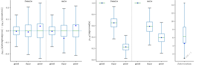
Figure 3: Box-plots on structural (dis)parity, confounder realism and interventional $OR$ calculated over $10^{6}$ three-way contingency tables that were sampled from the pr-projection provided in Table 2. Blue dots signify empirical estimates of the original study.

Our goal is again to examine the effectiveness of streptomycin in a hypothetical setting where ratio Eq. (27) equals unity for all profiles in $\mathcal{D}_{\boldsymbol{S}}$. This automatically balances the conditional distribution $\mathfrak{f}_{\boldsymbol{S}|X}$ in the two treatment groups via the observed marginal $\mathfrak{f}_{\boldsymbol{S}}$, as opposed to methods that deal independently with each potential confounder [44, 15]. Minimizing the $I$-divergence from $\mathfrak{f}$ under Eq. (9), as before, we obtain the unique distribution $\mathfrak{q}$ which satisfies structural parity,

$$Nq_{\boldsymbol{S}|X}(\boldsymbol{s}|x)=Nf_{\boldsymbol{S}}(\boldsymbol{s})=\,\begin{array}[]{l|ccc}&\texttt{good}&\texttt{fair}&\texttt{poor}\\ \cline{2-4}\cr\texttt{Female}&8&20&31\\ \texttt{Male}&8&17&23\end{array}\quad\text{for}\quad x\in\{\texttt{streptomycin},\texttt{control}\}$$ (32)

with group prevalences $N\mathfrak{q}_{X}(\texttt{control})=52$ and $N\mathfrak{q}_{X}(\texttt{streptomycin})=55$, as in the original data; alongside the Realism of $N\mathfrak{q}_{Y,\boldsymbol{S}}=N\mathfrak{f}_{Y,\boldsymbol{S}}$ obtained by adding row-wise the latter two columns in Table 2. Necessarily, the expected contingency table has fractional entries, e.g. $Nq_{X,\boldsymbol{S}}(\texttt{control},\texttt{Female},\texttt{good})=8\cdot 52/107\not\in\mathbb{Z}$ due to parity Eq. (32). Conceptually, this poses no problem, as $\mathfrak{q}$ expresses the mere expectation of the confounding-free scenario and not a particular study over $N$ subjects. The numerically determined $\mathfrak{q}$ self-consistently leads to the hypothetical

$$Intervention_{\mathfrak{q}}=\frac{Odds_{\mathfrak{q}}(\texttt{improved}|\texttt{streptomycin})}{Odds_{\mathfrak{q}}(\texttt{improved}|\texttt{control})\phantom{.........}}\approx 6.12$$ (33)

corresponding to an absolute risk reduction of more than $42\%$ in the streptomycin group. Therefore, enforcing structural parity seems to verify the conclusion of the original clinical trial on the significant improvement due to streptomycin medication.

Concerning three-factor effects, the $OR$ over the two groups for each patient profile $\boldsymbol{s}\in\mathcal{D}_{\boldsymbol{S}}$ from Eq. (22) remains unaltered by the pr-projection:

$$\frac{Odds_{\mathfrak{p}}(\texttt{improved}|\texttt{control},\texttt{gender},\texttt{baseline})\phantom{.........}}{Odds_{\mathfrak{p}}(\texttt{improved}|\texttt{streptomycin},\texttt{gender},\texttt{baseline})}=\,\begin{array}[]{l|ccc}&\texttt{good}&\texttt{fair}&\texttt{poor}\\ \cline{2-4}\cr\texttt{Female}&\text{undefined}&1/4&0\\ \texttt{Male}&\text{undefined}&1/9&0\end{array}\quad\text{for}\quad\mathfrak{p}=\mathfrak{f},\mathfrak{q}~{}.$$ (37)

On the other hand, the absolute risk reduction

$$ARR_{\mathfrak{p}}=\mathfrak{p}_{Y|X,\boldsymbol{S}}(\texttt{non-improved}|\texttt{control},\boldsymbol{s})-\mathfrak{p}_{Y|X,\boldsymbol{S}}(\texttt{non-improved}|\texttt{streptomycin},\boldsymbol{s})$$ (38)

experiences a slight change

$$ARR_{\mathfrak{f}}\approx\,\begin{array}[]{l|ccc}&\texttt{good}&\texttt{fair}&\texttt{poor}\\ \cline{2-4}\cr\texttt{Female}&0&30\%&41\%\\ \texttt{Male}&0&46\%&69\%\end{array}\quad\text{vs.}\quad ARR_{\mathfrak{q}}\begin{array}[]{l|ccc}&\texttt{good}&\texttt{fair}&\texttt{poor}\\ \cline{2-4}\cr\texttt{Female}&0&30\%&44\%\\ \texttt{Male}&0&48\%&76\%\end{array}$$ (45)

supporting the increased effectiveness of antibiotics in the hypothetical confounding-free scenario.

As a demonstration of the statistical nature of the pr approach, we generate from $\mathfrak{q}$ one million contingency tables with $N=107$ patients each. In Figure 3, we indeed recover parity and realism in expectation. Due to the estimation of fractional cell counts (noted below Eq. (32)), no single contingency table with the marginals $N\mathfrak{f}_{\boldsymbol{S}}$ and $N\mathfrak{f}_{X}$ of the original study could exactly reproduce the expectation about parity at the given sample size. Because of the small sample size, the range of fluctuations is also large. Conversely, increasing the sample size $N$ would concentrate all cell counts from the generated contingency tables around the expected values that can be directly read off from $N\mathfrak{q}$. In the last box-plot, we estimate the range of fluctuations at the given $N=107$ of the expected effect size Eq. (33) of intervention in the bias-free scenario.

3.3 Kidney stones

The clinical study [45] was designed to compare different methods of treating renal calculi. The treatment was defined as successful, if stones were eliminated or reduced to less than $2mm$ after three months. As it becomes clear from Table 3, the $N=985$ patients with renal calculi were distributed over treatment groups in an unbalanced way:

$$N\mathfrak{f}_{X}=\begin{array}[]{r|r}\texttt{ESWL}&328\\ \texttt{nephrolithotomy/pyelolithotomy}&231\\ \texttt{percutaneous\,\,nephrolithotomy}&350\\ \texttt{pyelolithotomy}&76\\ \end{array}~{}.$$ (50)

The same unbalanced trend applies for the proportion of patients with $s=\texttt{large}$ to $s=\texttt{small}$ stone size,

$$\frac{f_{S|X}(\texttt{large}|x)}{f_{S|X}(\texttt{small}|x)}\approx\begin{array}[]{r|r}\texttt{ESWL}&0.61\\ \texttt{nephrolithotomy/pyelolithotomy}&16.77\\ \texttt{percutaneous\,\,nephrolithotomy}&0.30\\ \texttt{pyelolithotomy}&1.45\\ \end{array}$$ (55)

within each treatment group $x$. Taking the most populous group as reference, we comparatively estimate the effect size of $Intervention_{\mathfrak{f}}$ as

$$\frac{Odds_{\mathfrak{f}}(\texttt{successful}|x)\phantom{percutaneous..nephrolithotomy}}{Odds_{\mathfrak{f}}(\texttt{successful}|\texttt{percutaneous\,\,nephrolithotomy})}\approx\begin{array}[]{r|r}\texttt{ESWL}&2.35\\ \texttt{nephrolithotomy/pyelolithotomy}&0.54\\ \texttt{pyelolithotomy}&1.13\\ \end{array}~{}.$$ (59)

Based on such $OR$, $x=\texttt{pyelolithotomy}$ would not show a significant improvement ($p\text{-value}\approx 0.87$) compared to $x_{0}=\texttt{percutaneous\,\,nephrolithotomy}$. In contrast, $x=\texttt{nephrolithotomy/pyelolithotomy}$ would appear significantly ($p\text{-value}\approx 0.003$) inferior to reference treatment, while $x=\texttt{ESWL}$ significantly ($p\text{-value}\approx 0.0004$) superior. These conclusions are significantly ($p\text{-value}<10^{-11}$) obfuscated by $S=\texttt{stone\,\,size}$,

$$\frac{Odds_{\mathfrak{f}}(\texttt{successful}|\texttt{small})}{Odds_{\mathfrak{f}}(\texttt{successful}|\texttt{large})}\approx 3.51$$ (60)

generically increasing the chances of successful outcome in patients with $s=\texttt{small}$. This significant influence of stone  size on the outcome had not been discovered and hence not accounted for in the original study design, as it becomes evident by Eq. (55).

$X=\texttt{treatment}$	$S=\texttt{stone\,\,size}$	$Y=\texttt{successful}$	empirical $N\mathfrak{f}$	pr-projection
		no	23	0.029433
extracorporeal shockwave	large	yes	101	0.128444
lithotripsy (ESWL)		no	4	0.003634
	small	yes	200	0.171484
		no	64	0.032787
nephrolithotomy/	large	yes	154	0.078401
pyelolithotomy		no	1	0.010006
	small	yes	12	0.113324
		no	25	0.052872
percutaneous	large	yes	55	0.115594
nephrolithotomy		no	36	0.026192
	small	yes	234	0.160672
		no	7	0.005721
	large	yes	38	0.030861
		no	5	0.006868
pyelolithotomy	small	yes	26	0.033708

Table 3: Three-way contingency table from the 1986 study on the effectiveness of different methods $x$ in treating renal calculi stratified by potential confounder $S$.

After eliminating structural differences among treatment groups,

$$\frac{q_{S|X}(\texttt{large}|x)}{q_{S|X}(\texttt{small}|x)}=\frac{f_{S}(\texttt{large})}{f_{S}(\texttt{small})}=\frac{467}{518}\approx 0.90\quad\forall\,\,x\in\mathcal{D}_{X}$$ (61)

the pr-projection of $\mathfrak{f}$ (last column in Table 3) re-evaluates Eq. (59) to

$$\frac{Odds_{\mathfrak{q}}(\texttt{successful}|x)\phantom{percutaneous..nephrolithotomy}}{Odds_{\mathfrak{q}}(\texttt{successful}|\texttt{percutaneous\,\,nephrolithotomy})}\approx\begin{array}[]{r|r}\texttt{ESWL}&2.60\\ \texttt{nephrolithotomy/pyelolithotomy}&1.28\\ \texttt{pyelolithotomy}&1.47\\ \end{array}~{}.$$ (65)

Given the hypothetical $OR$, we verify the significantly improving tendencies of $x=\texttt{ESWL}$ compared to $x_{0}$ from the original study. At the same time, $x=\texttt{pyelolithotomy}$ which appeared non-significant in the original data due to small ($n=76$) size, exhibits a potential to be found significant in future studies, as the confounding-free scenario $\mathfrak{q}$ raises its effectiveness. Finally, the significant inferiority of $x=\texttt{nephrolithotomy/pyelolithotomy}$ against $x_{0}$ previously detected by $\mathfrak{f}$ is entirely reversed in the confounding-free scenario (cf. Simpson’s paradox in Section 3.1).

All in one analysis, we manage with one fictitious-study distribution $\mathfrak{q}$ to exemplify all potential outcomes of a confounding-free scenario:

• verification of a previously significant outcome

• enhancement of a previously non-significant outcome

• complete overturning of the conclusion on the initial, confounded data

Based on the findings of the pr-projection, research questions regarding those four therapeutic strategies could have been modified or even entirely reformulated in subsequent studies.

3.4 COVID-19

Last but not least, we consider a more recent example from the covid-19 pandemic which demonstrates the power of our method to simultaneously deal with multiple intervention groups $|\mathcal{D}_{X}|>2$ and mutliple confounder profiles $|\mathcal{D}_{S}|>2$. The data, already investigated by [46] in a similar context, reports on $N=385\,925$ new covid-19 cases and deaths over the first wave until May 2020 in various countries stratified by $S=\texttt{age}$. Out of $82\,798$ confirmed fatalities, the research question with $\mathcal{D}_{Y}=\{\texttt{survived},\texttt{deceased}\}$ concerns the mortality rate of the pandemic in each $X=\texttt{country}$ from

$$\mathcal{D}_{X}=\left\{\texttt{Argentina},\texttt{Colombia},\texttt{Italy},\texttt{Netherlands},\texttt{South\,\,Africa},\texttt{South\,\,Korea},\texttt{Switzerland}\right\}~{}.$$ (66)

In a broader sense, the intervention in this application pertains to the impact on the mortality rate of various measures and living conditions aggregated by country. Essentially, we are interested to uncover what leads to discrepancies in the pandemic profile among different countries.

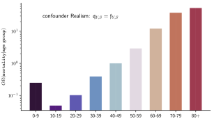
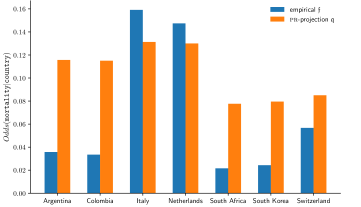
Figure 4: Left: global $OR$ for mortality due to covid-19 over the age groups as observed in the countries of the study ($s_{0}=\texttt{40-49}$ years as reference group). Right: mortality $Odds$ of covid-19 by country in 2020 empirically estimated by the official data $\mathfrak{f}$ (blue) and re-estimated by the pr-projection of $\mathfrak{f}$ (orange).

As widely known and verified [47], age poses a risk factor for covid-19 mortality. In the present dataset, this is manifested by the noteworthy association of mortality rate with the provided age groups in Figure 4 (left).

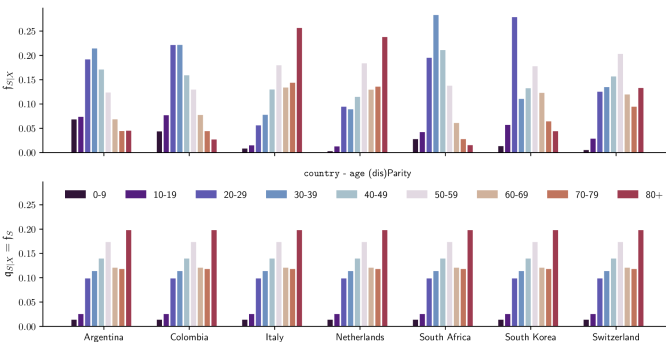
Figure 5: Upper: observed distribution of covid-19 cases over the age groups conditioned on the countries considered in the study. Lower: all considered countries share the same global distribution of cases over age groups in the hypothetical scenario of structural Parity.

However, not all countries exhibit the same distribution of covid-19 cases over age groups. This is exemplified by conditional $f_{S|X}(\texttt{age}|\texttt{country})$ for all age groups from 0-9 to 80+ in the upper bar diagram of Figure 5. Most strikingly, Italy and the Netherlands seem to have a significantly higher case rate in 80+ years with South  Africa exhibiting the lowest rate in this age group. Empirically, the resulting mortality by country can be quantified from $\mathfrak{f}$ via the

$$Odds_{\mathfrak{f}}(\texttt{mortality}|\texttt{country})=\frac{f_{Y|X}(\texttt{deceased}|\texttt{country})}{f_{Y|X}(\texttt{survived}|\texttt{country})}$$ (67)

which is depicted in the blue bar plot of Figure 4 (right).

Establishing parity in the age distribution of cases $q_{S|X}(\texttt{age}|\texttt{country})=f_{S}(\texttt{age})$ among each country leads to the hypothetical phenomenology of lower bar diagram 5. Since Italy had the highest incidence $f_{X}(\texttt{Italy})\approx 60\%$ in the dataset (followed by the Netherlands with almost $20\%$), the empirical marginal $f_{S}(\texttt{age})$ and hence also the hypothetical conditional $q_{S|X}(\texttt{age}|\texttt{country})$ are dominated by the profile of $f_{S|X}(\texttt{age}|\texttt{Italy})$. This adjustment for structural parity alongside the confounder realism of age as risk factor depicted in Figure 4 (left) lead to a new joint distribution $\mathfrak{q}$, the pr-projection of $\mathfrak{f}$, which re-estimates the $Odds$ of mortality by country Eq. (67) in the orange bar plot of Figure 4 (right).

Adjusting for structural parity, the $Odds$ for mortality significantly increase in countries where mostly younger covid-19 cases had been observed, while slightly decrease in European countries with a majority of older cases. After completely isolating the effect of age on mortality via the elimination of structural differences between countries regarding the profile of cases in Figure 5, we see a tendency of homogenizing the $Odds$ of mortality in each country (Figure 4, right). As anticipated, this alludes to age as a prominent risk factor for covid-19. However, the mortality rate does not become fully standardized in all investigated countries, as there exist further geographic-related factors that could play a role in the course of a disease, such as local history of past pandemics, social attitudes against covid-19, differences in health-care systems, case-report and death protocols.

4 Conclusions

In this work, we have argued in favor of top-down approach from the three-way contingency table between response $Y$, independent variables $\boldsymbol{X}$ and confounders $\boldsymbol{S}$ towards the elimination of confounder-induced bias in the response to an intervention/exposure. After deriving the expectation about the de-biased contingency table, any metric like $OR$, $RR$ and $ARR$ that quantifies the influence of the intervention on the outcome should be computed from the expected three-way table, otherwise it is usually meaningless. In that way, we avoid relying on external sources, special limits and model assumptions that generally perplex and – even most alarmingly – could bias our analysis in an uncontrolled way beyond information theory.

In a model-agnostic exploration fully compatible with TotEm, the minimization of $I$-divergence under structural parity proved to be a valuable tool. Through its unique solution, the pr-projection of $\mathfrak{f}$ gives us the mathematical guarantee that we do not unintentionally introduce any bias in our efforts to eliminate structural heterogeneity when going from empirical conditional $\mathfrak{f}_{\boldsymbol{S}|\boldsymbol{X}}$ towards the hypothetical $\mathfrak{p}_{\boldsymbol{S}|\boldsymbol{X}}=\mathfrak{f}_{\boldsymbol{S}}$. By doing so, we preserve – in expectation – as much of original data’s phenomenology as arithmetically feasible in a structurally homogeneous scenario. In latter scenario, any (non)-linear effect that might associate third-party variables $\boldsymbol{S}$ to the independent variables $\boldsymbol{X}$ has been, by construction, removed. In contrast to model-centric approaches that need to appeal to certain asymptotic limits presupposing conditions to be fulfilled by the data, the information-theoretic methodology of the pr-projection always achieves structural parity, as long as the suspected confounder profiles $\boldsymbol{s}$ are observed in all intervention groups $\boldsymbol{x}$.

The constrained $I$-divergence minimization in probability space leading to the pr-projection of the data elucidates that the optimization procedure of Section 2.1, which answers question 1, does not formally change with varying number of confounder manifestations and intervention groups, $|\mathcal{D}_{\boldsymbol{S}}|$ and $|\mathcal{D}_{\boldsymbol{X}}|$ respectively. Either we suspect multiple confounders (application 3.2) or deal with multiple groups (examples 3.3 and 3.4), the algorithmic procedure to obtain the pr-projection, which unambiguously predicts metrics for the interventional effect size ($OR$, $RR$, $ARR$) free from confounder-induced bias, formally remains the same. Furthermore, the utility of an information-theoretic methodology in data analysis also encompasses privacy-preserving aspects. Operating solely on contingency tables, namely summary statistics of microdata, which are provided in the original study, the pr-projection requires no additional input from individuals who may be unwilling to share sensitive information beyond the study’s scope. To summarize the pr projection gives the mathematical guarantee to

• learn confounder statistics and the realism of confounders’ influence on the outcome

• remove observed confounding by enforcing structural parity among intervention groups

• avoid unintentionally introducing additional bias in doing so

• uniquely re-estimate the effect size of the intervention in the confounding-free scenario

• be applicable in multi-arm studies, also in presence of multiple confounders

In [17], it was argued that a metric variable can be phenomenologically regarded as categorical. More precisely, we define any variable over a finite, categorical domain $\mathcal{D}_{\text{obs}}$ of its observed-only values incorporating the physical ordering of metric values through observed moments, which constrain the variable’s distribution over $\mathcal{D}_{\text{obs}}$. In future work, we plan to naturally extend the pr approach of eliminating structural differences over count and metric variables as well as adjust the pr-projection for survival analysis. In addition, we shall revisit modeling of relationships between attributes, both as a pre-processing step to counteract vanishing cells in contingency tables and as a post-processing step, after running the de-biasing to decide about significant trends in the structurally-homogeneous scenario.

Acknowledgments

We are thankful to Till Adhikary and Petros Marios Kitsaras for useful discussions as well as to Maria Chalkia for proofreading the manuscript.

References

- [1] Maria Blettner et al. “Traditional reviews, meta-analyses and pooled analyses in epidemiology.” In International journal of epidemiology 28.1, 1999, pp. 1–9
- [2] Jeffrey C Valentine and Simon G Thompson “Issues relating to confounding and meta-analysis when including non-randomized studies in systematic reviews on the effects of interventions” In Research synthesis methods 4.1 Wiley Online Library, 2013, pp. 26–35
- [3] Maya B Mathur and Tyler J VanderWeele “Sensitivity analysis for unmeasured confounding in meta-analyses” In Journal of the American Statistical Association Taylor & Francis, 2019
- [4] Maya B Mathur and Tyler J VanderWeele “Methods to address confounding and other biases in meta-analyses: review and recommendations” In Annual review of public health 43 Annual Reviews, 2022, pp. 19–35
- [5] Thomas D Cook, Donald Thomas Campbell and William Shadish “Experimental and quasi-experimental designs for generalized causal inference” Houghton Mifflin Boston, MA, 2002
- [6] Nicholas JS Christenfeld, Richard P Sloan, Douglas Carroll and Sander Greenland “Risk factors, confounding, and the illusion of statistical control” In Psychosomatic medicine 66.6 LWW, 2004, pp. 868–875
- [7] M Alan Brookhart et al. “Confounding control in healthcare database research: challenges and potential approaches” In Medical care 48.6 0 NIH Public Access, 2010, pp. S114
- [8] Orestis Loukas and Ho-Ryun Chung “Demographic Parity: Mitigating Biases in Real-World Data”, 2023 arXiv:2309.17347 [cs.LG]
- [9] Sander Greenland, Judea Pearl and James M Robins “Confounding and collapsibility in causal inference” In Statistical science 14.1 Institute of Mathematical Statistics, 1999, pp. 29–46
- [10] Tyler J VanderWeele “Principles of confounder selection” In European journal of epidemiology 34 Springer, 2019, pp. 211–219
- [11] Edwin T Jaynes “Probability theory: The logic of science” Cambridge university press, 2003
- [12] KJ Jager, C Zoccali, A Macleod and FW Dekker “Confounding: what it is and how to deal with it” In Kidney international 73.3 Elsevier, 2008, pp. 256–260
- [13] Steven Piantadosi “Clinical trials: a methodologic perspective” John Wiley & Sons, 2017
- [14] Nathan Mantel and William Haenszel “Statistical Aspects of the Analysis of Data From Retrospective Studies of Disease” In JNCI: Journal of the National Cancer Institute 22.4, 1959, pp. 719–748 DOI: 10.1093/jnci/22.4.719
- [15] Mohamad Amin Pourhoseingholi, Ahmad Reza Baghestani and Mohsen Vahedi “How to control confounding effects by statistical analysis” In Gastroenterology and hepatology from bed to bench 5.2 Shahid Beheshti University of Medical Sciences, 2012, pp. 79
- [16] M Soledad Cepeda, Ray Boston, John T Farrar and Brian L Strom “Comparison of logistic regression versus propensity score when the number of events is low and there are multiple confounders” In American journal of epidemiology 158.3 Oxford University Press, 2003, pp. 280–287
- [17] Orestis Loukas and Ho Ryun Chung “Total Empiricism: Learning from Data”, 2023 arXiv:2311.08315 [math.ST]
- [18] Weiwei Liu, S Janet Kuramoto and Elizabeth A Stuart “An introduction to sensitivity analysis for unobserved confounding in nonexperimental prevention research” In Prevention science 14 Springer, 2013, pp. 570–580
- [19] Alexander D’Amour “On multi-cause causal inference with unobserved confounding: Counterexamples, impossibility, and alternatives” In arXiv preprint arXiv:1902.10286, 2019
- [20] S. Kullback and R.. Leibler “On Information and Sufficiency” In The Annals of Mathematical Statistics 22.1 Institute of Mathematical Statistics, 1951, pp. 79–86 DOI: 10.1214/aoms/1177729694
- [21] Yurii Nesterov “Introductory lectures on convex optimization: A basic course” Springer Science & Business Media, 2003
- [22] Imre Csiszár “I-divergence geometry of probability distributions and minimization problems” In The annals of probability JSTOR, 1975, pp. 146–158
- [23] J Kruithof “Telefoonverkeersrekening” In De Ingenieur 52, 1937, pp. 15–25
- [24] Orestis Loukas and Ho Ryun Chung “Categorical Distributions of Maximum Entropy under Marginal Constraints”, 2022 arXiv:2204.03406 [hep-th]
- [25] Orestis Loukas and Ho Ryun Chung “Entropy-based Characterization of Modeling Constraints”, 2022 arXiv:2206.14105 [stat.ME]
- [26] E.. Jaynes “Concentration of Distributions at Entropy Maxima (1979)” In E. T. Jaynes: Papers on Probability, Statistics and Statistical Physics Dordrecht: Springer Netherlands, 1989, pp. 315–336 DOI: 10.1007/978-94-009-6581-2˙11
- [27] Orestis Loukas and Ho-Ryun Chung “Model Selection in the World of Maximum Entropy” In Physical Sciences Forum 5.1, 2022 DOI: 10.3390/psf2022005028
- [28] Darya Chyzhyk, Gaël Varoquaux, Michael Milham and Bertrand Thirion “How to remove or control confounds in predictive models, with applications to brain biomarkers” In GigaScience 11, 2022, pp. giac014 DOI: 10.1093/gigascience/giac014
- [29] Henry Bradford Smith “An Introduction to Logic and Scientific Method, by Morris R. Cohen and Ernest Nagel. New York: Harcourt, Brace and Co. 1934. xii, 467 pp.” In Philosophy of Science 1.4 Cambridge University Press, 1934, pp. 488–491 DOI: 10.1086/286347
- [30] G Udny Yule “Notes on the theory of association of attributes in statistics” In Biometrika 2.2 JSTOR, 1903, pp. 121–134
- [31] Edward H Simpson “The interpretation of interaction in contingency tables” In Journal of the Royal Statistical Society: Series B (Methodological) 13.2 Wiley Online Library, 1951, pp. 238–241
- [32] Robert E. Tarone “On summary estimators of relative risk” In Journal of Chronic Diseases 34.9, 1981, pp. 463–468 DOI: https://doi.org/10.1016/0021-9681(81)90006-0
- [33] Hisashi Noma and Kengo Nagashima “A Note on the Mantel-Haenszel Estimators When the Common Effect Assumptions Are Violated” In Epidemiologic Methods 5.1, 2016, pp. 19–35 DOI: doi:10.1515/em-2015-0004
- [34] John Shore and Rodney Johnson “Axiomatic derivation of the principle of maximum entropy and the principle of minimum cross-entropy” In IEEE Transactions on information theory 26.1 IEEE, 1980, pp. 26–37
- [35] Imre Csiszar “Why least squares and maximum entropy? An axiomatic approach to inference for linear inverse problems” In The annals of statistics 19.4 Institute of Mathematical Statistics, 1991, pp. 2032–2066
- [36] Richard Doll “Controlled trials: the 1948 watershed” In BMJ 317.7167 BMJ Publishing Group Ltd, 1998, pp. 1217–1220 DOI: 10.1136/bmj.317.7167.1217
- [37] Austin Bradford Hill “Medical Ethics and Controlled Trials” In BMJ 1.5337 BMJ Publishing Group Ltd, 1963, pp. 1043–1049 DOI: 10.1136/bmj.1.5337.1043
- [38] “STREPTOMYCIN treatment of pulmonary tuberculosis” In British medical journal 2.4582, 1948, pp. 769–782
- [39] Peter Higgins “Reproducible Medical Research with R” R package version 0.2.0, 2021 URL: https://higgi13425.github.io/medicaldata/index.html
- [40] John Crofton “The MRC Randomized Trial of Streptomycin and its Legacy: A View from the Clinical front Line” PMID: 17021304 In Journal of the Royal Society of Medicine 99.10, 2006, pp. 531–534 DOI: 10.1177/.014107680609901017
- [41] Yvonne M Bishop, Stephen E Fienberg and Paul W Holland “Discrete multivariate analysis: theory and practice” Springer Science & Business Media, 2007
- [42] W.F. Rosenberger and J.M. Lachin “Randomization in Clinical Trials: Theory and Practice”, Wiley Series in Probability and Statistics Wiley, 2015 URL: https://books.google.de/books?id=ZJEvCgAAQBAJ
- [43] David L. Demets “Methods for combining randomized clinical trials: Strengths and limitations” In Statistics in Medicine 6.3, 1987, pp. 341–348 DOI: https://doi.org/10.1002/sim.4780060325
- [44] Rolf HH Groenwold, Olaf H Klungel, Diederick E Grobbee and Arno W Hoes “Selection of confounding variables should not be based on observed associations with exposure” In European journal of epidemiology 26 Springer, 2011, pp. 589–593
- [45] C.. Charig, D.. Webb, S.. Payne and J… Wickham “Comparison Of Treatment Of Renal Calculi By Open Surgery, Percutaneous Nephrolithotomy, And Extracorporeal Shockwave Lithotripsy” In British Medical Journal (Clinical Research Edition) 292.6524 BMJ, 1986, pp. 879–882 URL: http://www.jstor.org/stable/29522724
- [46] Julius Kügelgen, Luigi Gresele and Bernhard Schölkopf “Simpson’s Paradox in COVID-19 Case Fatality Rates: A Mediation Analysis of Age-Related Causal Effects” In IEEE Transactions on Artificial Intelligence 2.1, 2021, pp. 18–27 DOI: 10.1109/TAI.2021.3073088
- [47] Karla Romero Starke et al. “The isolated effect of age on the risk of COVID-19 severe outcomes: a systematic review with meta-analysis” In BMJ Global Health 6.12 BMJ Specialist Journals, 2021 DOI: 10.1136/bmjgh-2021-006434