Sparse Projected Averaged Regression for High-Dimensional Data

Abstract

We examine the linear regression problem in a challenging high-dimensional setting with correlated predictors to explain and predict relevant quantities, with explicitly allowing the regression coefficient to vary from sparse to dense. Most classical high-dimensional regression estimators require some degree of sparsity. We discuss the more recent concepts of variable screening and random projection as computationally fast dimension reduction tools, and propose a new random projection matrix tailored to the linear regression problem with a theoretical bound on the gain in expected prediction error over conventional random projections.

Around this new random projection, we built the Sparse Projected Averaged Regression (SPAR) method combining probabilistic variable screening steps with the random projection steps to obtain an ensemble of small linear models. In difference to existing methods, we introduce a thresholding parameter to obtain some degree of sparsity.

In extensive simulations and two real data applications we guide through the elements of this method and compare prediction and variable selection performance to various competitors. For prediction, our method performs at least as good as the best competitors in most settings with a high number of truly active variables, while variable selection remains a hard task for all methods in high dimensions.

Keywords High-Dimensional Regression  $\cdot$ Dimension Reduction  $\cdot$ Random Projection  $\cdot$ Screening

1 Introduction

The recent advances in technology have allowed more and more quantities to be tracked and stored, which has lead to a huge increase in the amount of data, making available datasets more complex and larger than ever, both in dimension and size. We consider a standard linear regression setting, where the response variable is given by

$$y_{i}=\mu+x_{i}^{\prime}\beta+\varepsilon_{i},\quad i=1,\dots,n.$$ (1)

Here, $n$ is the number of observations, $\mu$ is a deterministic intercept, the $x_{i}$s are iid observations of $p$-dimensional covariates or predictors with common covariance matrix $\Sigma\in\mathbb{R}^{p\times p}$, $\beta=(\beta_{1},\dots,\beta_{p})^{\prime}\in\mathbb{R}^{p}$ is an unknown parameter vector and the $\varepsilon_{i}$s are iid error terms with $\mathbb{E}[\varepsilon_{i}]=0$ and constant $\text{Var}(\varepsilon_{i})=\sigma^{2}$ independent from the $x_{i}$s. We are interested in studying the case where $p>n$ or even $p\gg n$.

Most of the literature dealing with this setting imposes certain sparsity assumptions on the regression coefficient $\beta$ (see, e.g., Fan and Lv, 2010). It is very unlikely to obtain theoretical guarantees without additional assumptions. For example, Wainwright (2019) show that there is no consistent estimator when $p/n$ is bounded away from $0$ for general $\beta$.

We explicitly do not want to impose any sparsity assumption and allow the number of active variables $a=|\{j:\beta_{j}\neq 0,1\leq j\leq p\}|$ to be larger than $n$ up to a fraction of $p$, and we are interested in methods with good prediction ability which are also able to identify the true active variables. Recent work addressing both a sparse and dense setting in high-dimensional regression include Silin and Fan (2022) and Gruber and Kastner (2023).

Although many classical methods, like partial least squares (PLS), principal component regression (PCR), Elastic Net (Zou and Hastie, 2005) or adaptive LASSO (Zou, 2006), could still be applied in the investigated setting, Hastie et al. (2009, Chapter 18) mention that such methods designed for $p<n$ might behave differently in high dimensions.

A more recent tool for dimension reduction in the high-dimensional regression setting is the idea of variable screening, where a subset of variables is selected for further analysis or modeling, and the other variables are disregarded. A seminal work in this field is Sure Independence Screening (SIS) by Fan and Lv (2007), where the variables with highest absolute correlation to the response are selected. Other important papers include Forward Regression Screening (Wang, 2009) and High-Dimensional Ordinary Least Squares Projection (HOLP; Wang and Leng, 2015).

Another tool used for dimension reduction in statistics and machine learning is random projection. Random projection first came up in the area of compression to speed up computation and save storage. Possible applications are low-rank approximations (Clarkson and Woodruff, 2013), data reduction for high $n$ (e.g. Geppert et al., 2015), or data privacy (e.g. Zhou et al., 2007). It has also been applied to project the predictors to a random lower dimensional space in linear regression models to obtain predictive models, see e.g Maillard and Munos (2009) and Guhaniyogi and Dunson (2015). Thanei et al. (2017) discuss the application of random projection for column-wise compression in linear regression problems and give an overview of theoretical guarantees on generalization error.

Even though many papers include desirable theoretical asymptotic properties for these random dimension reduction techniques, it might be beneficial in practice to combine information of multiple such reductions in practice in order to account for the uncertainty in the random reductions. Targeted Random Projection (TARP; Mukhopadhyay and Dunson, 2020) combines a probabilistic screening step with random projection and averages over multiple replications of this procedure to obtain predictions.

Our main contributions in this work are threefold.

• We propose a new random projection designed for dimension reduction in linear regression, which takes the variables’ effect on the response into consideration, and give a theoretical bound on the expected gain in prediction error compared to a conventional random projection.

• Using this new random projection, we build the Sparse Projected Averaged Regression (SPAR) method, which combines an ensemble of screened and projected linear models and adds sparsity by introducing a threshold parameter.

• In a broad simulation study across six different covariance structures and three different levels of sparsity, we benchmark this new approach against an extensive collection of existing methods and point out possible performance gains.

The paper is organized as follows. Section 2 introduces the methodology with one section dedicated to variable screening and one to the new random projection, before we combine them in one method. An extensive simulation study is presented in Section 3. Section 4 illustrates the proposed method on two real world datasets (rat eye gene expression and angles of face images), and Section 5 concludes.

2 Methods

In this section, we first introduce the concept of variable screening and motivate the use of HOLP over SIS for this purpose. Then, we present conventional random projections before proposing our own random projection tailored to dimension reduction for linear regression and giving a theoretical bound on the performance gain in expected prediction error. Finally, we discuss how to combine these two concepts and propose our own algorithm.

The following notation is used throughout the rest of this paper. For any integer $n\in\mathbb{N}$, $[n]$ denotes the set $\{1,\dots,n\}$, $I_{n}\in\mathbb{R}^{n\times n}$ is the $n$-dimensional identity matrix and $1_{n}\in\mathbb{R}^{n}$ is an $n$-dimensional vector of ones. From model (1), we let $X\in\mathbb{R}^{n\times p}$ be the matrix of centered predictors with rows $\{x_{i}-\bar{x}:i\in[n]\}$ and $y=(y_{1}-\bar{y},\dots,y_{n}-\bar{y})^{\prime}\in\mathbb{R}^{n}$ the centered response vector, where $\bar{x}=\frac{1}{n}\sum_{i=1}^{n}x_{i}\in\mathbb{R}^{p},\bar{y}=\frac{1}{n}\sum_{i=1}^{n}y_{i}\in\mathbb{R}$. Furthermore, $X_{.j}=(X_{1j},\dots,X_{nj})^{\prime}\in\mathbb{R}^{n}$ denotes $j$-th columns of $X$.

2.1 Variable Screening

The general idea of variable screening is to select a (small) subset of variables, based on some marginal utility measure for the predictors, and disregard the rest for further analysis. In their seminal work, Fan and Lv (2007) propose to use the vector of marginal empirical correlations $w=(w_{1},\ldots,w_{p})^{\prime}\in\mathbb{R}^{p},w_{j}=\text{Cor}(X_{.j},y)$ for variable screening by selecting the variable set $\mathcal{A}_{\gamma}=\{j\in[p]:|w_{j}|>\gamma\}$ depending on a threshold $\gamma>0$, where $[p]=\{1,\dots,p\}$. Under certain technical conditions, where $p$ grows exponentially with $n$, they show that this procedure has the sure screening property

$$\mathbb{P}(\mathcal{A}\subset\mathcal{A}_{\gamma_{n}})\to 1\text{ for }n\to\infty$$ (2)

with an explicit exponential rate of convergence, where $\mathcal{A}=\{j\in[p]:\beta_{j}\neq 0\}$ is the set of truly active variables. These conditions imply that $\mathcal{A}$ and $\mathcal{A}_{\gamma_{n}}$ contain less than $n$ variables. One of the critical conditions is that, on the population level for some fixed $i\in[n]$,

$$\min_{j\in\mathcal{A}}|\text{Cov}(y_{i}/\beta_{j},x_{ij})|\geq c$$ (3)

for some constant $c>0$, which rules out practically possible scenarios where an important variable is marginally uncorrelated to the response.

If we want a screening measure for marginal variable importance considering the other variables in the model, one natural choice in a usual linear regression model with $p<n$ would be the least-squares estimator $\hat{\beta}=(X^{\prime}X)^{-1}X^{\prime}y$. The Ridge estimator $\hat{\beta}_{\lambda}=(X^{\prime}X+\lambda I_{p})^{-1}X^{\prime}y$, can be seen as a compromise between the two, since $\lim_{\lambda\to 0}\hat{\beta}_{\lambda}=\hat{\beta}$ and $\lim_{\lambda\to\infty}\lambda\hat{\beta}_{\lambda}=X^{\prime}y$. It can also be used in the case $p>n$ and has the alternative form (see Lemma 2)

$$\hat{\beta}_{\lambda}=X^{\prime}(\lambda I_{n}+XX^{\prime})^{-1}y,$$ (4)

which is especially useful for saving computational complexity for very large $p$, since the inverted matrix only has dimension $n\times n$, bringing down the computational complexity to $\mathcal{O}(n^{2}p)$ (Wang and Leng, 2015). If we now let $\lambda\to 0$, assuming $\text{rank}(XX^{\prime})=n$ and therefore $p>n$, we end up with the HOLP estimator from Wang and Leng (2015)

$$\hat{\beta}_{HOLP}=X^{\prime}(XX^{\prime})^{-1}y=\lim_{\lambda\to 0}\hat{\beta}_{\lambda},$$ (5)

which is also the minimum norm solution to $X\beta=y$ (see Lemma 3). Kobak et al. (2020) show that the optimal Ridge penalty for minimal mean-squared prediction error can be zero or negative for real world high-dimensional data, because low-variance directions in the predictors can already provide an implicit Ridge regularization.

This motivates choosing the absolute values of the tuning-free coefficient vector $\hat{\beta}_{\text{HOLP}}$ for variable screening. Under similar conditions as in Fan and Lv (2007), but without assumption (3) on the marginal correlations to the response, and allowing $p>c_{0}n$ with $c_{0}>1$ to grow at any rate, Wang and Leng (2015) show that $\hat{\beta}_{\text{HOLP}}$ also has the sure screening property. Furthermore, they show screening consistency of the estimator for exponential growth of $p$, meaning that

$$\mathbb{P}\Big{(}\min_{j\in\mathcal{A}}|\hat{\beta}_{\text{HOLP},j}|>\max_{j\notin\mathcal{A}}|\hat{\beta}_{\text{HOLP},j}|\Big{)}\to 1\text{ for }n\to\infty$$ (6)

at an exponential rate. This means that, asymptotically, the $a=|\mathcal{A}|$ highest absolute coefficients of $\hat{\beta}_{\text{HOLP}}$ correspond exactly to the true active variables.

In another work, Wang et al. (2015) derive and compare the requirements for SIS and HOLP screening to have the strong screening consistency

$$\min_{j\in\mathcal{A}}|\hat{\beta}_{j}|>\max_{j\notin\mathcal{A}}|\hat{\beta}_{j}|\quad\text{ and }\quad\text{sign}(\hat{\beta}_{j})=\text{sign}(\beta_{j})\quad\forall j\in\mathcal{A},$$ (7)

where $\hat{\beta}$ is an estimator of the true $\beta$. Both methods are shown to be strongly screening consistent with large probability when the sample size is of order $n=\mathcal{O}\big{(}(\rho a+\sigma/\tau)^{2}\log(p)\big{)}$, where $\tau=\min_{j\in\mathcal{A}}|\beta_{j}|$ measures the signal strength and $\rho=\max_{j\in\mathcal{A}}|\beta_{j}|/\tau$ measures the diversity of the signals. However, for SIS the predictor covariance matrix $\Sigma$ needs to satisfy the restricted diagonally dominant (RDD) condition given in Wang et al. (2015, Definition 3.1), which is related to the irrepresentable condition (IC) of Zhao and Yu (2006) for model selection consistency of the LASSO. This excludes certain settings, while for HOLP only the condition number $\kappa$ of the covariance matrix enters the required sample size as a constant, meaning it is always screening consistent for a large enough sample size.

In the calculation of $\hat{\beta}_{\text{HOLP}}$ there might be a problem when $p$ is close to $n$ or $XX^{\prime}$ is close to degeneracy, which can lead to a blow-up of the error term. In the discussion, Wang and Leng (2015) recommend to use the Ridge coefficient $\hat{\beta}_{\lambda}=X^{\prime}(\lambda I_{n}+XX^{\prime})^{-1}y$ with penalty $\lambda=\sqrt{n}+\sqrt{p}$ in this case to control the explosion of the noise term.

So far, we have shown theoretical foundations for HOLP and SIS screening. Now we also want to look at the practical performance in a quick simulation example. The simulation study provided in Wang and Leng (2015) focuses on correctly selecting a sparse true model, while we are also interested in the HOLP estimator being almost proportional to the true regression coefficients $\beta$ for later application in the random projection.

Therefore, we simulate data similar to later in Section 3.1 from the following example used throughout this section.

Example 1.

We generate data from (1) with multivariate normal predictors $x_{i}\sim N(0,\Sigma)$ and normal errors $\varepsilon_{i}\sim N(0,\sigma^{2})$, where we choose $n=200,p=2000,a=100,\mu=1$, and $\Sigma=\rho 1_{p}1_{p}^{\prime}+(1-\rho)I_{p}$ has a compound symmetry structure with $\rho=0.5$ and eigenvalues $\lambda_{1}=1-\rho+p\rho,\lambda_{j}=1-\rho,j=2,\dots,p$. The first $a=100$ entries of $\beta$ are uniformly drawn from $\pm\{1,2,3\}$ and the rest are zero. The error variance $\sigma^{2}$ is chosen such that the signal-to-noise ratio is $\rho_{\text{snr}}=\beta^{\prime}\Sigma\beta/\sigma^{2}=10$.

We compare variable screening based on the marginal correlations, HOLP, Ridge with proposed penalty $\lambda=\sqrt{n}+\sqrt{p}$ and Ridge with $\lambda$ chosen by $10$-fold cross-validation. Figure 1(a) shows density estimates of the absolute coefficients estimated by these four methods for truly active and non-active variables for $100$ replicated draws of the data. In Figure 1(b) we evaluate the selection process of the four methods when selecting the $k$ variables having the highest absolute estimated coefficients and let $k$ vary on the x-axis. We show the precision and recall of this selection, as well as the ratio of correct sign for truly active predictors included in the selection and the correlation of the corresponding true coefficients to the estimates, averaged over the $100$ replications. We see that HOLP and Ridge with penalty $\lambda=\sqrt{n}+\sqrt{p}$ better separate the active and non-active predictors and achieve better results for precision, recall, true sign recovery and correlation to the true coefficient compared to Ridge with cross-validated penalty and correlation-based screening. In Figure 1(a), we see that the absolute coefficients of cross-validated Ridge are much smaller than HOLP and Ridge with $\lambda=\sqrt{n}+\sqrt{p}$, meaning the $\lambda$ suggested by cross-validation is much higher. In comparison, the choice $\lambda=\sqrt{n}+\sqrt{p}$ even leads to quite similar results as HOLP, which can be interpreted as Ridge with $\lambda=0$.

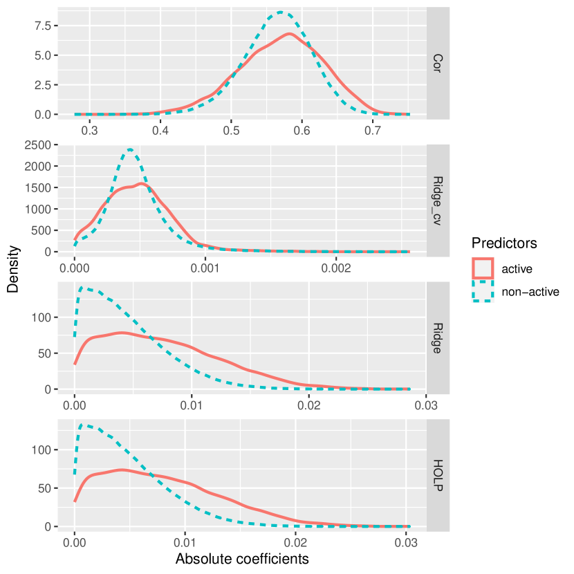
(a) Density estimates of absolute coefficients

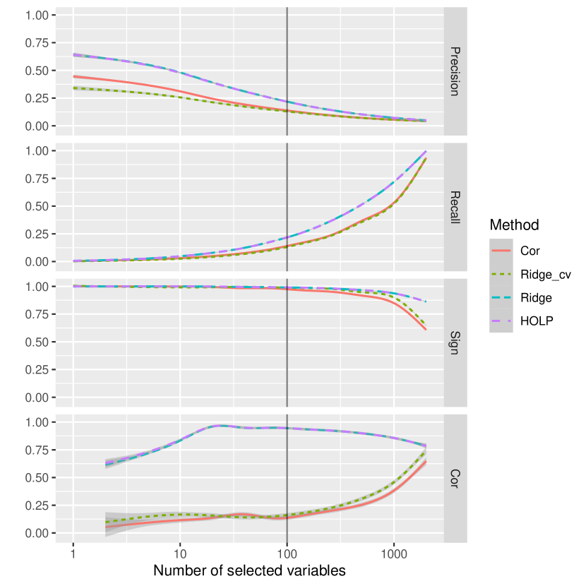
(b) Screening measures

Figure 1: Comparison of screening based on marginal correlations, HOLP, Ridge with $\lambda=\sqrt{n}+\sqrt{p}$ and Ridge with cross-validated $\lambda$ in the setting $n=200,p=2000,a=100,\Sigma=0.5\cdot 1_{p}1_{p}^{\prime}+0.5\cdot I_{p}$ and $\rho_{\text{snr}}=10$, where (a) shows density estimates of absolute estimated coefficients for active and non-active predictors of $100$ draws of the data, and (b) shows precision, recall, and sign recovery and correlation of estimates to the true coefficients averaged over $100$ replications, where the vertical line at $a=100$ indicates the true number of active variables

2.2 Random Projection

Random projection is used as a dimension reduction tool in high-dimensional statistics by creating a random matrix $\Phi\in\mathbb{R}^{m\times p}$ with $m\ll p$ and using the reduced predictors $z_{i}=\Phi x_{i}\in\mathbb{R}^{m}$ for further analysis. When applying it to linear regression, we would wish that the reduced predictors still have most of the predictive power and that $\beta\in\text{span}(\Phi^{\prime})$, such that the true coefficients can still be recovered after the reduction.

Random projections first became popular after Johnson and Lindenstrauss (1984), hereafter abbreviated by JL, who proved the existence of a linear map that approximately preserves pairwise distances for a set of points in high dimensions in a much lower-dimensional space. Many papers followed, giving explicit constructions of a random matrix $\Phi\in\mathbb{R}^{m\times p}$ satisfying this JL property with high probability. The classic construction is setting the elements of this matrix $\Phi_{ij}\overset{iid}{\sim}N(0,1)$ (Frankl and Maehara, 1988), but also sparse versions with iid entries

$$\Phi_{ij}=\begin{cases}\pm 1/\sqrt{\psi}&\text{with prob. }\psi/2\\ 0&\text{with prob. }1-\psi\end{cases},$$ (8)

for $0<\psi\leq 1$ can satisfy the property after appropriate scaling. Achlioptas (2003) gave the results for $\psi=1$ or $\psi=1/3$, and even sparser choices such as $\psi=1/\sqrt{p}$ or $\psi=\log(p)/p$ were later shown to be possible with little loss in accuracy of preserving distances (Li et al., 2006).

In this section, we propose a new random projection matrix tailored to the regression problem. We start from a sparse embedding matrix $\Phi\in\mathbb{R}^{m\times p},m\ll p$ from Clarkson and Woodruff (2013), which can be used to form a random projection with the JL property and is obtained in the following way.

Definition 1.

Let $h:[p]\to[m]$ be a random map such that for each $j\in[p]:h(j)=h_{j}\overset{iid}{\sim}\text{Unif}([m])$. Let $B\in\mathbb{R}^{m\times p}$ be a binary matrix with $B_{h_{j},j}=1$ for all $j\in[p]$ and remaining entries $0$, where we assume $\text{rank}(B)=m$. Let $D\in\mathbb{R}^{p\times p}$ be a diagonal matrix with entries $d_{j}\sim\text{Unif}(\{-1,1\}),j\in[p]$ independent of $h$. Then we call $\Phi=BD$ a CW random projection.

Each variable $j$ is mapped to a uniformly random goal dimension $h_{j}$ with random sign. We assume that each goal dimension $k\in[m]$ is attained by $h$ for some variable $j\in[p]$, which leads to $\text{rank}(B)=m$. Otherwise we just discard this dimension and reduce $m$ by one. When using this random projection for our linear regression problem (1), variables in the same goal dimension should not have signs conflicting their respective influence on the response, and, in general, we would wish for $\beta\in\text{span}(\Phi^{\prime})$ such that the true coefficients $\beta\in\mathbb{R}^{p}$ can be recovered by the reduced predictors $z_{i}=\Phi x_{i}$ when modeling the responses as their linear combination $y_{i}\approx z_{i}^{\prime}\gamma=x_{i}^{\prime}\Phi^{\prime}\gamma,\gamma\in\mathbb{R}^{m}$.

Lemma 4 shows that for a CW random projection $\Phi$ with general diagonal entries $d_{j}\in\mathbb{R}$, the projection of a general $\beta\in\mathbb{R}^{p}$ to the row-span of $\Phi$ given by $\tilde{\beta}=P_{\Phi}\beta=\Phi^{\prime}(\Phi\Phi^{\prime})^{-1}\Phi~\beta$ can be explicitly expressed as

$$\tilde{\beta}_{j}=d_{j}\cdot\frac{\sum_{k:h_{k}=h_{j}}d_{k}\beta_{k}}{\sum_{k:h_{k}=h_{j}}d_{k}^{2}}.$$

Therefore, we propose to set $d_{j}=c\cdot\beta_{j}$ for some constant $c\in\mathbb{R}$. We obtain $\tilde{\beta}=\beta$ and therefore $\beta\in\text{span}(\Phi^{\prime})$. The following theorem shows that we can improve the mean square prediction error when using these diagonal elements proportional to $\beta$ instead of using random signs.

Theorem 1.

Assume we have data $(y_{i},x_{i}),i=1,\dots,n$ from the model

$$y_{i}=x_{i}^{\prime}\beta+\varepsilon_{i},i=1,\dots,n,$$ (9)

where $x_{i}\overset{iid}{\sim}N(0,\Sigma)$ with $0<\Sigma\in\mathbb{R}^{p\times p},p>n$ and the $\varepsilon_{i}$s are iid error terms with $\mathbb{E}[\varepsilon_{i}]=0$ and constant $\text{Var}(\varepsilon_{i})=\sigma^{2}$ independent of the $x_{i}$s, and we want to predict a new observation from the same distribution $\tilde{y}=\tilde{x}^{\prime}\beta+\tilde{\varepsilon}$ independent from the given data. For a smaller dimension $m<n-1$, let $\Phi_{\text{rs}}=BD_{\text{rs}}\in\mathbb{R}^{m\times p}$ be the CW random projection with random sign diagonal entries and $\Phi_{\text{pt}}=BD_{\text{pt}}\in\mathbb{R}^{m\times p}$ the CW random projection with diagonal entries $d_{j}^{\text{pt}}=c\beta_{j}$ for some constant $c>0$ proportional to the true coefficient $\beta$. We assume that for each $i\in[m]$ there is a $j\in h^{-1}(i)=\{k\in[p]:h(k)=i\}$ with $\beta_{j}\neq 0$. Otherwise, in order to retain $\text{rank}(\Phi_{\text{pt}})=m$, we set $j_{i}=\min(h^{-1}(i))$ and $d_{j_{i}}^{\text{pt}}=\text{Unif}(\{-1,1\})\cdot\min_{j:d_{j}^{\text{pt}}\neq 0}|d_{j}^{\text{pt}}|$ for each $i\in[m]$ where it does not hold.

For $X\in\mathbb{R}^{n\times p}$ with rows $\{x_{i}\}_{i=1}^{n}$ and $y=(y_{1},\dots,y_{n})^{\prime}\in\mathbb{R}^{n}$, let $Z_{\text{rs}}=X\Phi_{\text{rs}}^{\prime}\in\mathbb{R}^{n\times m}$ and $Z_{\text{pt}}=X\Phi_{\text{pt}}^{\prime}\in\mathbb{R}^{n\times m}$ be the reduced predictor matrices and $\hat{y}_{\text{rs}}=(\Phi_{\text{rs}}\tilde{x})^{\prime}(Z_{\text{rs}}^{\prime}Z_{\text{rs}})^{-1}Z_{\text{rs}}^{\prime}y$ and $\hat{y}_{\text{pt}}=(\Phi_{\text{pt}}\tilde{x})^{\prime}(Z_{\text{pt}}^{\prime}Z_{\text{pt}})^{-1}Z_{\text{pt}}^{\prime}y$ the corresponding least-squares predictions. Then,

$$\mathbb{E}[(\tilde{y}- \hat{y}_{\text{rs}})^{2}]-\mathbb{E}[(\tilde{y}-\hat{y}_{\text{pt}})^{2}]\geq C_{\text{Th1}}>0,$$ (10)

$$C_{\text{Th1}} =\|\beta\|^{2}\Bigl{[}\lambda_{p}(1-\frac{2m}{p})\Bigr{]}+\frac{a}{p-1}m\lambda_{p}\tau^{2}(1-\frac{m+1}{p-1}+\mathcal{O}(p^{-2})),$$ (11)

where $\mathcal{A}=\{j\in[p]:\beta_{j}\neq 0\}$ is the active index set, $a=|\mathcal{A}|$ is the number of active variables, $\tau=\min_{j:\beta_{j}\neq 0}|\beta_{j}|$ is the smallest non-zero absolute coefficient and $\lambda_{p}>0$ is the smallest eigenvalue of $\Sigma$.

The proof can be found in Appendix A.

Remark 1.

• This theorem shows that when using a conventional random projection from Definition 1 for least-squares regression, the expected squared prediction error is much smaller when using diagonal elements proportional to the variables’ true effect to the response as opposed to the conventional random sign, and gives an explicit conservative lower bound on how much smaller it has to be at least.

• In practice, the true $\beta$ is unknown, but in Section 2.1 we saw that $\hat{\beta}_{\text{HOLP}}$ asymptotically recovers the true sign and order of magnitude with high probability, and has high correlation to the true $\beta$, meaning it is ’almost’ proportional to the true $\beta$. So we propose to use $\hat{\beta}_{\text{HOLP}}$ as diagonal elements of our projection. See Remark 2 in Appendix A for a short note on the implications on the error bound, the relaxation of distributional assumptions and the full-rank adaption of $\Phi_{\text{pt}}$.

• Note that this bound is non-asymptotic and valid for any allowed $m,n,p,a$ (up to the quadratic order in $p$), and it does not depend on the signal-to-noise ratio $\rho_{\text{snr}}$ or the noise level $\sigma^{2}$, because they have the same average effect on the error for both random projections.

In the following, we want to verify above considerations and the obtained bound by evaluating the prediction performance of different projections in a small simulation example, where we use the setting from Example 1 again. When $\Phi\in\mathbb{R}^{m\times p}$ is the selected random projection matrix, we fit an ordinary least-squares model to the responses $y_{i}$ on the reduced predictors $z_{i}=\Phi x_{i}$ to obtain predictions for $n_{test}=100$ new predictor observations. These predictions are evaluated by the mean squared prediction error MSPE. We set the reduced dimension to the true number of active variables $m=a=100$ and compare $\Phi$ chosen Gaussian with iid $N(0,1)$ entries, Sparse from (8) with $\psi=1/3$, and the following three versions from our Definition 1: SparseCW with standard random sign diagonal elements, SparseCWSign with $d_{j}=\text{sign}(\hat{\beta}_{\text{HOLP},j})$ and SparseCWHolp with $d_{j}=\hat{\beta}_{\text{HOLP},j}$. Additionally, we look at regression with HOLP, which uses the full predictors, and two oracles SparseCWSignB from Definition 1 with $d_{j}=\text{sign}(\beta)$ and SparseCWBeta with $d_{j}=\beta_{j}$ with the full-rank adaptions proposed in Theorem 1. Figure 2 shows prediction performance of these different projections and HOLP for $100$ replications. We also plot the theoretical lower bound $C_{\text{Th1}}$ from Theorem 1 from the best oracle to SparseCW with random signs and see that the difference is actually higher. The conventional random projections stay well above this bound, while our proposed random projections using the HOLP-coefficient manage to stay within the bound to the oracle’s performance. SparseCWHolp is able to produce predictions that are as good as the ones from the HOLP model using all variables, and for both the oracle and our proposed random projection using the sign-information instead of the coefficients performs similar but slightly worse.

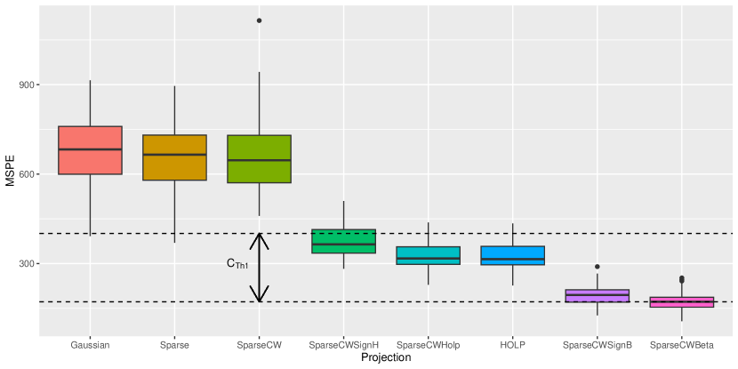
Figure 2: Comparison of prediction performance of different conventional projections, our proposed projection using the HOLP coefficient or its signs, HOLP and the oracle projections using the true $\beta$ or its signs for $100$ replications of the setting of Example 1 with $n=200,p=2000,m=a=100$ and $\Sigma=0.5\cdot 1_{p}1_{p}^{\prime}+0.5\cdot I_{p}$

2.3 Combination of Screening and Random Projection

Previous work by Mukhopadhyay and Dunson (2020) in this area showed that it can be beneficial to combine these two tools for dimension reduction by using a probabilistic variable screening step first, keeping only the more important ones, and then performing random projection on these remaining variables. Repeating these steps many times and averaging results can reduce dependence on the random projection and increase prediction performance. After explaining their methods in more detail, we will propose our adaptions of the procedure and investigate different combinations of screening and random projection and the effect of the number of screened variables.

In more detail, Mukhopadhyay and Dunson (2020) propose to include each variable with probability

$$q_{j}=\frac{|\text{Cor}(x_{ij},y_{i})|^{\nu}}{\max_{k}|\text{Cor}(x_{ik},y_{i})|^{\nu}},\quad\nu>0,\text{ some }i\in[n]$$

with $\nu=(1+\log(p/n))/2$, and use a random dimension $m\sim\text{Unif}(\{2\log(p),\dots,3n/4\})$ for a general sparse projection of type (8). With this choice, the variable with highest marginal importance is always included and the number of screened variables is not directly controlled. There is no explicit discussion on the number of models used, but Guhaniyogi and Dunson (2015) report that the gains are diminishing after using around $100$ models for averaging.

Instead, we propose to set the number of screened variables to a fixed multiple of the sample size $c\cdot n$ (independent of $p$), and drawing the variables with probabilities proportional to their marginal utility based on the HOLP-estimator $p_{j}\propto|\hat{\beta}_{\text{HOLP},j}|$, as well as using slightly smaller goal dimensions $m\sim\text{Unif}(\{\log(p),\dots,n/2\})$ to increase estimation performance of the linear regression in the reduced model, and our proposed random projection from Definition 1 with the entries of $\hat{\beta}_{\text{HOLP}}$ corresponding to the screened variables as diagonal elements. These steps are explained more rigorously in Section 2.4.

We go back to our data setting from Example 1 and want to examine the effects of the number of marginal models for different combinations of variable screening and random projection for our proposed adaptations. Figure 3 shows the effect of the number of models used on the average prediction performance over $100$ replications and compares the following four methods: screening to $n/2$ variables based on $\hat{\beta}_{\text{HOLP}}$ (Scr_HOLP), random projections with SparseCW matrix (RP_CW) and our proposed SparseCWHolp matrix (RP_CWHolp), and first screening with $\hat{\beta}_{\text{HOLP}}$ to $2n$ variables and then using the SparseCWHolp random projection (ScrRP). When we use just one model, the screening methods deterministically select the variables with highest marginal importance $|\hat{\beta}_{\text{HOLP},j}|,j=1,\dots,p$, otherwise they are drawn with probabilities $p_{j}\propto|\hat{\beta}_{\text{HOLP},j}|$, as previously mentioned. We can see that the combination of screening and random projection yields the best performance and the effect of using more models diminishes at around $20$ models already for this method.

In Figure 4 we look at the effect of the number of screened variables $c\cdot n$ on prediction performance, where we compare just screening (Scr_HOLP) to the combination of screening with random projection (ScrRP) as above for fixed number of models $M=20$, and we show again averages over $100$ replications. For just screening we use the HOLP estimator from Section 2.1 as the subsequent regression method when $c\geq 1$, and in case the system is close to degeneracy we add a small ridge penalty $\lambda=0.01$ to the OLS estimate. We see that the screening still has bad performance for $c$ close to $1$, because the sample covariance of the selected predictors is close to singularity. For small and large ratio’s it achieves better prediction performance. When combining the screening with the random projection, $c$ does not have such a huge impact, and we can achieve lower prediction errors where the best results are achieved for $2\leq c\leq 4$.

So far, every variable selected once in the screening step will have some contribution in the final regression coefficient, so when we choose a smaller number of used models and ratio $c$, there will be less variables involved, and in the following Section 2.4 we will use a thresholding step to actively set less important contributions to $0$ to obtain some level of sparsity.

When combining the predictions of different models, there are many different ways to choose their respective model weights, such as AIC (Burnham and Anderson, 2004), prediction error (leave-out-one or cross-validation), true posterior model weights in a Bayesian approach or dynamic model weights in time series modeling (Gruber and Kastner, 2023). Also, we could try to use a subset of all models considering their performance according to their weight and also the diversity of the combined models (Reeve and Brown, 2018). However, across all our efforts in this area, the simple average across all models turned out to yield the best predictions most consistently for different settings. This observation was already reported in the literature as the forecast combination puzzle (Claeskens et al., 2016).

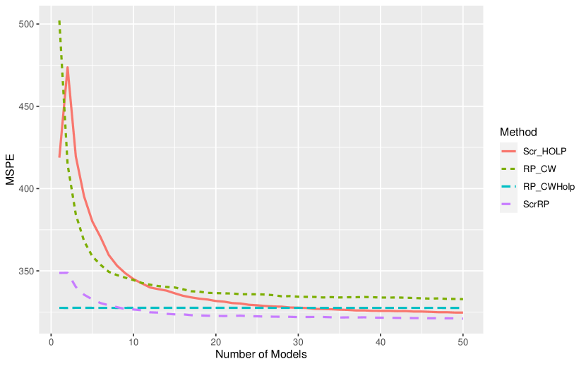
Figure 3: Average mean squared prediction error for different combinations of screening and random projection over the used number of models for $100$ replications of the setting from Example 1 with $n=200,p=2000,m=a=100$ and $\Sigma=0.5\cdot 1_{p}1_{p}^{\prime}+0.5\cdot I_{p}$

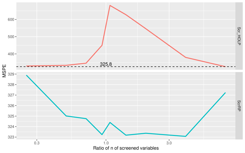
Figure 4: Average effect of number of screened variables on mean squared prediction error of only screening compared to screening plus random projection before fitting linear regression model for $100$ replications of the setting of Example 1 with $n=200,p=2000,m=r=100$ and $\Sigma=0.5\cdot 1_{p}1_{p}^{\prime}+0.5\cdot I_{p}$

2.4 Sparse Projected Averaged Regression (SPAR)

The considerations of the previous sections lead us to propose the following algorithm for high-dimensional regression where $p>n$.

1. standardize inputs $X:n\times p$ and $y:n\times 1$

2. calculate $\hat{\beta}_{\text{HOLP}}=X^{\prime}(XX^{\prime})^{-1}y$

3. For $k=1,\dots,M$:

   • draw $2n$ predictors with probabilities $p_{j}\propto|\hat{\beta}_{\text{HOLP},j}|$ yielding screening index set $I_{k}=\{j_{1}^{k},\dots,j_{2n}^{k}\}\subset[p]$

   • project remaining variables to dimension $m_{k}\sim\text{Unif}\{\log(p),\dots,n/2\}$ using $\Phi_{k}:m_{k}\times 2n$ from Definition 1 with diagonal elements $d_{i}=\hat{\beta}_{\text{HOLP},j_{i}^{k}}$ to obtain reduced predictors $Z_{k}=X_{.I_{k}}\Phi_{k}^{\prime}\in\mathbb{R}^{n\times m_{k}}$

   • fit OLS of $y$ against $Z_{k}$ to obtain $\gamma^{k}=(Z_{k}^{\prime}Z_{k})^{-1}Z_{k}^{\prime}y$ and $\hat{\beta}^{k}$, where $\hat{\beta}_{I_{k}}^{k}=\Phi_{k}^{\prime}\gamma^{k}$ and $\hat{\beta}_{\bar{I}_{k}}^{k}=0$.

4. for a given threshold $\lambda>0$, set all entries $\hat{\beta}_{j}^{k}$ with $|\hat{\beta}_{j}^{k}|<\lambda$ to $0$ for all $j,k$

5. combine via simple average $\hat{\beta}=\sum_{k=1}^{M}\hat{\beta}^{k}/M$

6. choose $M$ and $\lambda$ via $10$-fold cross-validation by repeating steps 1 to 5 (but with using the original index sets $I_{k}$ and projections $\Phi_{k}$) for each fold and evaluating the prediction performance by MSE on the withheld fold; choose either

   $$(M_{\text{best}},\lambda_{\text{best}})=\text{argmin}_{M,\lambda}\widehat{\text{MSE}}(M,\lambda),$$ (12)

   or

   $$(M_{\text{1-se}},\lambda_{\text{1-se}}) =\text{argmin}_{M,\lambda}\{|\{j:\hat{\beta}_{j}(M,\lambda)\neq 0\}|:\widehat{\text{MSE}}(M,\lambda)\leq$$

   $$\qquad\qquad\widehat{\text{MSE}}(M_{\text{best}},\lambda_{\text{best}})+se(\widehat{\text{MSE}}(M_{\text{best}},\lambda_{\text{best}}))\}.$$ (13)

7. output the estimated coefficients and predictions for the chosen $M$ and $\lambda$

We use the following notation in step 3. For a vector $y\in\mathbb{R}^{n}$ and an index set $I\subset[n]$, $\bar{I}$ denotes the complement, $y_{I}\in\mathbb{R}^{|I|}$ denotes the subvector with entries $\{y_{i}:i\in I\}$, and for a matrix $B\in\mathbb{R}^{n\times m}$, $B_{I.}\in\mathbb{R}^{|I|\times m}$ denotes the submatrix with rows $\{B_{i.}:i\in I\}$ and similarly for a subset of the columns.

The standardization in step 1 helps to stabilize computation and makes the estimated regression coefficients comparable for variable selection. The thresholding step 4 introduces sparsity to the otherwise dense estimator, because many variables will be selected by the random screening at least once. After this step, we only keep the most significant contributions, where the threshold-level can be selected via cross-validation. We can select the $\lambda$ which achieves the smallest MSE, or the $\lambda$ which leads to the least estimated active predictors, but still has MSE within one standard error of the best MSE. The number of marginal models $M$ could also be chosen via cross-validation (after specifying a maximum number), but in practice (e.g. Figure 3) we saw that the effect of $M$ deteriorates once it is high enough, and it suffices to set $M=20$.

3 Simulation Study

This section compares different aspects of our proposed SPAR method to several competitors in an extensive simulation study. First, we explain the data generation setting including six different covariance structures and coefficient settings, ranging from sparse (few truly active variables) to dense (many active variables). Then, we define the used evaluation measures and list all considered competitors, before presenting the results in Section 3.4.

3.1 Data Generation

We generate $n=200$ observations from a linear model

$$y_{i}=\mu+x_{i}^{\prime}\beta+\varepsilon_{i},\quad i=1,\dots,n,$$ (14)

where $\mu$ is a deterministic constant, the $x_{i}\sim N_{p}(0,\Sigma)$ follow an iid $p$-variate normal distribution, and $\varepsilon_{i}\sim N(0,\sigma^{2})$ are iid error terms independent from the $x_{i}$s. The covariance matrix $\Sigma$ of the predictors and the coefficient vector $\beta\in\mathbb{R}^{p\times p}$ will change depending on the simulation setting. The mean is set to $\mu=1$ and the error variance $\sigma^{2}$ is chosen such that the signal-to-noise ratio $\rho_{snr}$

$$\rho_{snr}=\frac{\text{Var}(\mu+x^{\prime}\beta)}{\text{Var}(\varepsilon)}=\frac{\beta^{\prime}\Sigma\beta}{\sigma^{2}}$$

is equal to $10$. We choose $p=2000$ as a high number of variables and consider the following different simulation settings for $\Sigma$. The choice of the number of truly active variables $a$ and their coefficients $\beta$ will be explained below.

1. Independent predictors: $\Sigma=I_{p}$.

2. Compound symmetry structure: $\Sigma=\rho 1_{p}1_{p}^{\prime}+(1-\rho)I_{p}$, where we set $\rho=0.5$.

3. Autoregressive structure: The $(i,j)$-th entry is given by $\Sigma_{ij}=\rho^{|i-j|}$ and we choose $\rho=0.9$. This structure is appropriate if there is a natural order among the predictors and two predictors with larger distance are less correlated, e.g. when they give measurements over time.

4. Group structure: Similarly to scheme II in Mukhopadhyay and Dunson (2020), $\Sigma$ follows a block-diagonal structure with blocks of $100$ predictors each, where the first half of the blocks has the compound structure from setting 2 and the second half has the AR structure from setting 3. Only the very last block has identity structure corresponding to independent predictors within that block, and the predictors between different blocks are independent.

5. Factor model: Inspired by model 4.1.4. in Wang and Leng (2015), we first generate a $p\times k$ factor matrix $F$ with $k=a$ and iid standard normal entries, and then set $\Sigma=FF^{\prime}+0.01\cdot I_{p}$. Here, dimension reduction of the predictors will be useful, because most of the information lies within the $k$-dimensional subspace defined by $F$.

6. Extreme correlation: Similarly to example 4 in Wang (2009), we create each predictor variable $x_{i}$ the following way.

   For $i=1,\dots,n$, let $z_{ij}\sim N(0,1)$ be iid standard normal variables for $j=1,\dots,p$ and $w_{ij}\sim N(0,1)$ iid standard normal variables for $j=1,\dots,a$ independent of the $z_{ij}$s. We then set

   $$x_{ij}=\begin{cases}(z_{ij}+w_{ij})/\sqrt{2}&j\leq a\\ (z_{ij}+\sum_{k=1}^{a}z_{ik})/\sqrt{m+1}&j>a\end{cases}.$$

We vary $a$ between a sparse $a=2\log(p)$, medium $a=n/2+2\log(p)$ and dense $a=p/4$ choice (rounded to closest integer). For settings 1 to 5, the positions of the non-zero entries in $\beta$ are chosen uniform random (without replacement) in $[p]$ and these entries are independently set as $(-1)^{u}(4\log(n)/\sqrt{n}+|z|)$, where $u$ is drawn from a Bernoulli distribution with probability of success parameter $p=0.4$ and $z$ is a standard normal variable. This choice was taken from Fan and Lv (2007), such that the coefficients are bounded away from $0$ and vary in sign and magnitude.

In setting 6, we choose the first $a$ predictors to be active with $\beta_{j}=j$ for $j=1,\dots,m$ and $\beta_{k}=0$ for $k>a$. In this setting it is extremely difficult to find any true active predictor, since the marginal correlation of any active predictor $x_{j},j\leq a$ to the response is way smaller than that of any unimportant predictor $x_{k},k>a$. In fact, the exact ratio between them is $(j/a)\cdot 2^{-3/2}\cdot(a+1)^{-1/2}<1$ for $j=1,\dots,a$.

For each setting we generate $n=200$ observations and evaluate the performance on $n_{\text{test}}=100$ further test observations. For setting 4, we also consider $p=500,10000$, $n=100,400$ as well as $\rho_{\text{snr}}=1,5$, and each setting is repeated $n_{\text{rep}}=100$ times. In the following section we will introduce the used error measures.

3.2 Error Measures

We evaluate prediction performance on $n_{test}=100$ independent observations via relative mean squared prediction error

$$\text{rMSPE}=\sum_{i=1}^{n_{test}}(\hat{y}_{i}^{test}-y_{i}^{test})^{2}\Big{/}\sum_{i=1}^{n_{test}}(y_{i}^{test}-\bar{y})^{2},$$ (15)

which is also used and motivated in Silin and Fan (2022). This measure scales the mean squared error by the error of a naive estimator $\hat{\beta}=0$, which can also achieve a small mean squared error in some high-dimensional settings, in the sense that it is close to zero for growing sample size and dimension. Therefore, this measure gives an interpretable performance measure relative to the naive estimator $\hat{\beta}=0$ and we want to achieve $\text{rMSPE}<1$ as small as possible.

For the evaluation of variable selection, which is a hard task in this high-dimensional setting, we let $\mathcal{A}\subset[p]$ denote the index set of truly active variables of size $|\mathcal{A}|=a$. Then, precision, recall, and F1 score are defined as

precision $$=\frac{\sum_{j=1}^{p}I\{\beta_{j}\neq 0,\hat{\beta}_{j}\neq 0\}}{\sum_{j=1}^{p}I\{\hat{\beta}_{j}\neq 0\}},$$ (16)

recall $$=\frac{\sum_{j=1}^{p}I\{\beta_{j}\neq 0,\hat{\beta}_{j}\neq 0\}}{\sum_{j=1}^{p}I\{\beta_{j}\neq 0\}}=\frac{\sum_{j\in\mathcal{A}}I\{\hat{\beta}_{j}\neq 0\}}{a},$$ (17)

F1 $$=2\cdot\frac{\text{precision}\cdot\text{recall}}{\text{precision}+\text{recall}}.$$ (18)

High precision and high recall are both worth striving for, however, there are rarely methods that excel in both. The F1 score combines these two into one measure to evaluate a method’s ability to identify true active variables. Furthermore, we also report the estimated number of active predictors for the different methods.

3.3 Competitors

We compare the following set of methods.

1. HOLP (Wang and Leng, 2015)

2. AdLASSO using 10-fold CV (Zou, 2006),

3. Elastic Net with $\alpha=3/4$ using 10-fold CV (Zou and Hastie, 2005),

4. SIS (Fan and Lv, 2007, screening method)

5. TARP (Mukhopadhyay and Dunson, 2020, random projection method),

6. SPAR CV with fixed $M=20$ and both best $\lambda$ and 1-se $\lambda$

HOLP is a method for a non-sparse, i.e. dense, setting, because all estimated regression coefficients are non-zero, and does, therefore, not perform any variable selection. The TARP method, in the way it is provided, does not return estimated regression coefficients, but in principle each variable that is selected at least once in the screening will have non-zero coefficient and the method is therefore not suitable for variable selection as well. Methods 2 to 4 do perform variable selection and return sparse regression coefficients. They will by marked by dotted boxes in the following Figures.

We also implemented PLS, PCR and Ridge, but we omit them from the results for a more compact overview. They all resulted in a prediction performance similar to HOLP, or slightly worse, and they are also all dense methods not useful for variable selection.

All methods were implemented in R (R Core Team, 2022) using the packages glmnet (Friedman et al., 2010, AdLASSO and ElNet), SIS (Saldana and Feng, 2018), and the source code available online on https://github.com/david-dunson/TARP for TARP. Our proposed method is implemented in the R-package SPAR available on github (https://github.com/RomanParzer/SPAR).

3.4 Results

First, we look at the prediction results of the competing methods for the six different covariance settings and sparse, medium and dense setting for the active variables with fixed $n=200,p=2000,\rho_{\text{snr}}=10$ in Figure 5. We see that the overall performance depends heavily on the covariance setting, and the signal-to-noise ratio alone does not quantify the difficulty of a regression problem. In the ’independent’ covariance setting with many active predictors, all methods barely outperform the naive estimator $\hat{\beta}=0$ with a rMSPE close to one, while in other covariance settings the errors are much lower. In general, we see that the sparse methods, especially AdLASSO and ElNet, perform well in sparse settings, but not in settings with more active variables. On the other hand, the HOLP method performs well in all dense settings, but is much worse than other methods in sparse settings. Our proposed SPAR method seem to be less dependent on the active variable setting and can provide useful predictions in all three cases, with slightly better results in more dense cases.

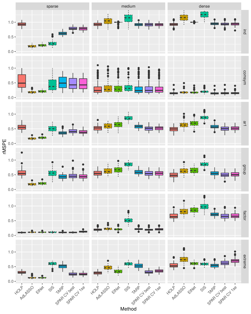
Figure 5: Relative mean squared prediction errors of the competing methods, where the sparse methods are marked by dotted boxes, for the six different covariance settings and sparse, medium and dense setting for the active variables for $n_{\text{rep}}=100$ replications ($n=200,p=2000,\rho_{\text{snr}}=10$)

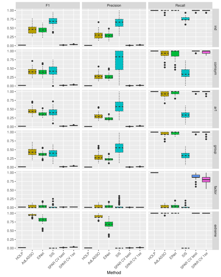
Figure 13: Precision, recall and F1 score of the competing methods, where the sparse methods are marked by dotted boxes, for the six different covariance settings and sparse setting for the active variables for $n_{\text{rep}}=100$ replications ($n=200,p=2000,\rho_{\text{snr}}=10$)

Figure 6 shows precision, recall and F1 score of all competitors (except TARP, see remark in Section 3.3) for the same covariance structures and medium setting for the active variables. The sparse methods do achieve higher precision, while the dense methods reach higher recall. However, no method achieves a good combined F1 score in most settings, which suggests that variable selection in high dimensions is a very hard task. Interestingly, the ’extreme’ covariance setting is the only setting where some methods achieve good F1 scores. This setting was designed to make it hard for methods using marginal correlations of predictors to the response, and we can see that SIS does not select any true active variables. However, SIS and TARP, which also relies on marginal correlations, still achieve acceptable prediction performance for many active variables in this covariance setting in Figure 5. These results also suggest that SPAR behaves more like a dense method. For completeness, Figures 13 and 14 in the appendix show the results for the same covariance settings, but for sparse and dense active variable settings. One interesting result is that ’SPAR 1-se’ is the only method with a high F1 score in the dense ’extreme’ covariance setting.

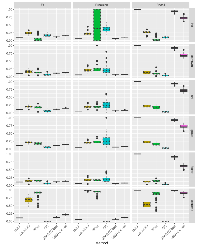
Figure 6: Precision, recall and F1 score of the competing methods, where the sparse methods are marked by dotted boxes, for the six different covariance settings and medium setting for the active variables for $n_{\text{rep}}=100$ replications ($n=200,p=2000,\rho_{\text{snr}}=10$)

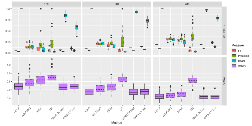
Figure 15: Performance measures of the competing methods, where the sparse methods are marked by dotted boxes, for ’group’ covariance setting, medium setting for the active variables and $n=100,200,400$ for $n_{\text{rep}}=100$ replications ($p=2000,\rho_{\text{snr}}=10$)

Next, we take a closer look at the most general ’group’ covariance setting with medium active variables and look at the effect of changing $p,n$ or $\rho_{\text{snr}}$. Figure 7 shows that all methods achieve increasingly better performance measures when $p$ is decreasing. A similar effect can be seen for increasing $n$ and for increasing signal-to-noise ratio $\rho_{\text{snr}}$ (see Figures 15 and 16 in Appendix), where both versions of SPAR are always among the best methods for prediction.

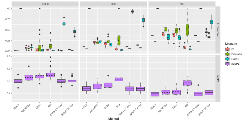
Figure 7: Performance measures of the competing methods, where the sparse methods are marked by dotted boxes, for ’group’ covariance setting, medium setting for the active variables and $p=500,2000,10000$ for $n_{\text{rep}}=100$ replications ($n=200,\rho_{\text{snr}}=10$)

Figure 8 shows the average computing times in the ’group’ covariance setting. All used methods scale quite well with $p$, where SIS and HOLP take the least time to compute. Even with the cross-validation procedure, our SPAR method takes similar computing time to well-established methods such as AdLASSO.

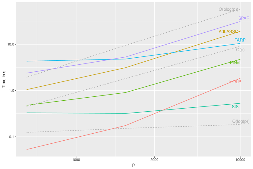
Figure 8: Average computing time in seconds in the ’group’ covariance setting over $n_{\text{rep}}=100$ replications of each active variable setting for increasing $p$ and fixed $n=200,\rho_{\text{snr}}=10$.

4 Data Applications

In this section, we now want to apply our proposed SPAR method and the same competitors to two real world high-dimensional regression problems, where one could be regarded as a sparse problem and the other one as rather dense. For both applications we randomly split the data into training set of size $3n/4$ and test set of size $n/4$ (rounded) for evaluation and repeat this process $n_{\text{rep}}=100$ times.

4.1 Rateye Gene Expression

This dataset was obtained for a study by Scheetz et al. (2006), where they collected tissues from eyes of $n=120$ rats and measured expression levels of $31042$ (non-control) gene probes. One of these genes, TRIM32, was identified as an additional BBS (Bardet-Biedl syndrome, multisystem human disease) gene (Chiang et al., 2006). It is now interesting to model the relation of all other genes to TRIM32 in order to find other possible BBS genes. Since only a few genes are expected to be linked to the given gene, this can be interpreted as a sparse high-dimensional regression problem (Huang et al., 2006). Similarly to Huang et al. (2006) and Scheetz et al. (2006), we only use genes that are expressed in the eye and have sufficient variation for our analysis. A gene is expressed, if its maximum observed value is higher than the first quartile of all expression values of all genes, and has sufficient variation, if it exhibits at least two-fold variation. For us, $p=22905$ filtered genes meet these criteria to be used in our analysis. This dataset is also available in the R-package flare (Li et al., 2022) with a different subset of $p=200$ genes, where all but $3$ are also contained in our filtered version. The selection process is not described in any more detail, but all $200$ selected genes have higher marginal correlation to TRIM32 than three quarters of all available genes.

Figure 9 shows the prediction performance for these two versions of the dataset, where HOLP, TARP and ‘SPAR best’ perform best on the bigger dataset. Interestingly, the sparse methods achieve better performance on the smaller version of the dataset compared to the full filtered dataset, while the others are able to reach better prediction performance from the bigger dataset.

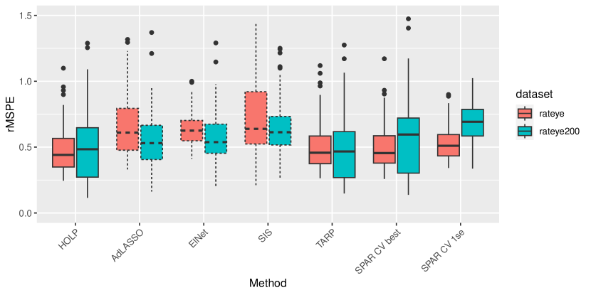
Figure 9: Relative mean squared prediction errors of the competing methods, where the sparse methods are marked by dotted boxes, on the two rat eye gene expression datasets for $n_{\text{rep}}=100$ random training/test splits

Table 1 shows the median number of active variables of the competing methods on these data applications, confirming the simulation results that our SPAR method uses more active variables than sparse methods. Evaluating variable selection in this real world application, where the truth is unknown, is very difficult. In the Appendix Section C, we compare which genes are selected by each of our competitors. Our ’SPAR best’ method offers a compromise of strong prediction performance on the same level as the best methods, with some level of sparsity, since it used only around $3200$ of the $22905$ genes on average. The fact that any sparse method, even just using the one standard error rule instead of the best $\lambda$ in the cross-validation in SPAR for more sparsity, achieves worse prediction performance, raises the question whether this problem is actually sparse. In simulated sparse settings, the sparse methods always performed better than the rest.

4.2 Face Images

The second dataset originates from Tenenbaum et al. (2000) and was also studied, among others, in Guhaniyogi and Dunson (2016). It consists of $n=698$ black and white face images of size $p=64\times 64=4096$ and the faces’ horizontal looking direction angle as response. The bottom left plot in Figure 11 illustrates one such instance with the corresponding angle. For each training/test split, we exclude pixels close to the edges and corners, which are constant on the training set. This example was previously used for non-linear methods in (low-dimensional) manifold regression, but in a linear model many pixels together carry relevant information, making this a rather dense regression problem.

Figure 10 shows our prediction performance results for this dataset. Here, HOLP and ‘SPAR best’ yield the lowest prediction error, while AdLASSO and SIS perform substantially worse than the others. Their number of active predictors used seems to be just too low to capture the information of the faces’ looking direction, see Table 1.

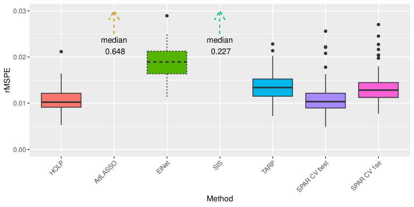
Figure 10: Relative mean squared prediction errors of the competing methods, where the sparse methods are marked by dotted lines, on the face angle dataset for $n_{\text{rep}}=100$ random training/test splits

For this dataset, we can also nicely illustrate the estimated regression coefficients and their contribution to a new prediction for our method SPAR with threshold $\lambda$ selected by the one-standard-error rule. We apply our method once on the full dataset except for two test images, thus $n=696$. The top of Figure 11 shows the positive (left) and negative (right) estimated regression coefficients of the pixels. It yields almost symmetrical images, which is sensible, and highlights the contours of the nose and forehead. For the prediction of a new face image, we can define the contribution of each pixel as the pixel’s regression coefficient multiplied by the corresponding pixel grey-scale value of the new instance. In the bottom right we visualize these contributions for one of the two new test instances on the bottom left. The sum of all these contribution (plus a ’hidden’ intercept) yields the prediction of $\hat{y}=34.8$ for the true angle $y=35.2$.

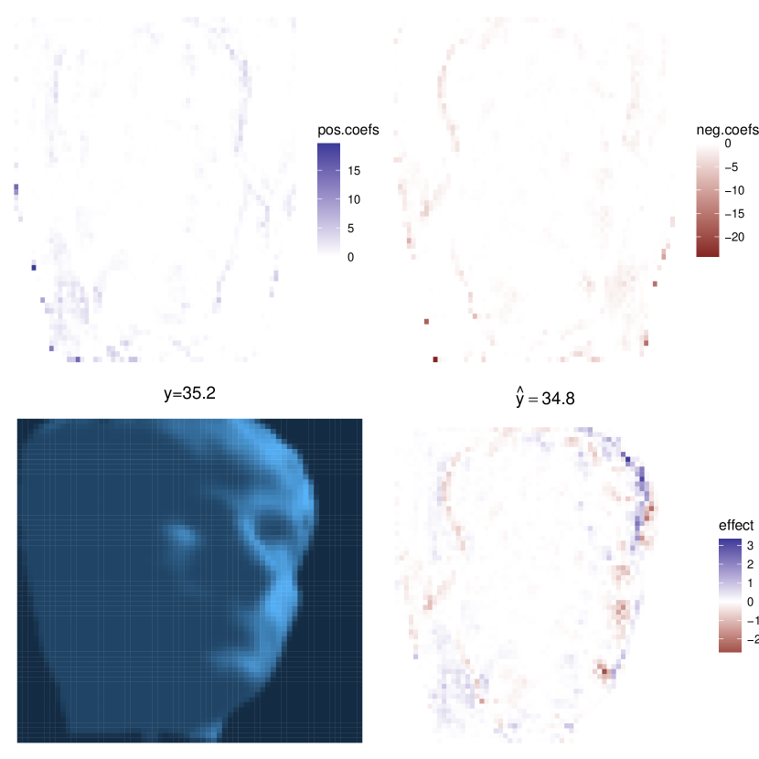
Figure 11: Top: positive (left) and negative (right) estimated regression coefficients of ’SPAR 1-se’, Bottom: One new instance (left) and the contributions of each pixel to its prediction (right)

Figure 12 illustrates the threshold selection of our SPAR method for this application, where we see the mean squared error estimated by cross-validation and the corresponding error band on the top, and the implied number of active variables on the bottom, over a grid of $\lambda$-values (displayed as rounded to three digits). With almost the same estimated prediction error, the ‘SPAR 1-se’ method uses over $1000$ pixels less than ‘SPAR best’. For the previous data application, the difference is even more severe, as shown in Table 1.

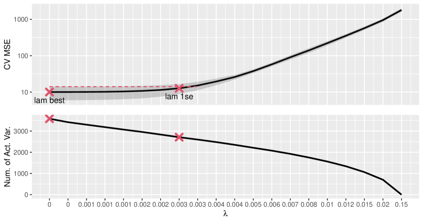
Figure 12: Mean squared prediction error estimated by cross-validation (and one standard-error band) on top and the corresponding number of active predictors (bottom) over a grid of $\lambda$-thresholds (displayed as rounded to three digits) for SPAR method on face angle data

Table 1: Median number of active predictors for all methods on data applications across $n_{\text{rep}}=100$ random training/test splits

Method	rateye	rateye200	face
HOLP	22905.0	200.0	3890.0
AdLASSO	46.0	10.0	19.0
ElNet	24.0	19.0	113.5
SIS	5.0	4.0	6.0
SPAR CV best	3203.5	193.0	3482.5
SPAR CV 1se	1038.5	95.5	2422.0

5 Summary and Conclusions

In this paper, we introduced a new ’data-informed’ random projection aimed at dimension reduction for linear regression, which uses the HOLP estimator (Wang and Leng, 2015) from variable screening literature, together with a theoretical result showing how much better we can expect the prediction error to be compared to a conventional random projection.

Around this new random projection, we built the SPAR ensemble method with a data-driven threshold selection introducing sparsity. We propose two different choices for this threshold. Firstly, the value providing the smallest cross-validated MSE, and secondly, the value leading to the sparsest coefficient while still achieving a similar cross-validated MSE. The first one should be chosen when purely predictions are of interest. In case we want to interpret the model and identify important variables, the second version should be prefered. SPAR is able the bridge the gap between sparse and non-sparse methods to some extent, since it achieves similar performance to the best non-sparse methods in medium and dense settings and beats them in sparse settings. However, as shown in our simulations, in very sparse settings, the data and MSE-driven threshold selection leads to too many active variables, and sparse methods end up performing better both for prediction and variable selection. How to modify the method to detect the right degree of sparsity is an open problem, if such a degree can even be determined in real-world problems. In non-sparse high-dimensional settings, we saw that no method performed well overall for variable selection, indicating the difficulty of this task.

This methodology can be extended to non-linear (or robust) regression by employing non-linear (or robust) methods, such as generalized linear models or Gaussian processes, in the marginal models instead of OLS. Possible future work also includes finding a similar adaption of conventional random projections useful for classification tasks.

Declarations

Roman Parzer and Laura Vana-Gür acknowledge funding from the Austrian Science Fund (FWF) for the project “High-dimensional statistical learning: New methods to advance economic and sustainability policies” (ZK 35), jointly carried out by WU Vienna University of Economics and Business, Paris Lodron University Salzburg, TU Wien, and the Austrian Institute of Economic Research (WIFO).

Appendix A Lemmas and Proof of Theorem 1

This section states and proves Lemmas 2, 3 and 4 mentioned in Section 2, and gives a detailed proof of Theorem 1 and Lemma 5 needed in the proof.

Lemma 2.

Let $X\in\mathbb{R}^{n\times p}$ be a fixed matrix and $y\in\mathbb{R}^{n}$ a vector. Then, the Ridge estimator for $\lambda>0$ has the following alternative form suitable for the $p\gg n$ case.

$$\hat{\beta}_{\lambda} :=(X^{\prime}X+\lambda I_{p})^{-1}X^{\prime}y=X^{\prime}(\lambda I_{n}+XX^{\prime})^{-1}y$$ (19)

Proof.

Using the Woodbury matrix inversion formula

$$(A+UCV)^{-1}=A^{-1}-A^{-1}U(C^{-1}+VA^{-1}U)^{-1}VA^{-1},$$

where $A$, $U$, $C$ and $V$ are conformable matrices, we have for any penalty $\lambda>0$

$$\hat{\beta}_{\lambda} :=(X^{\prime}X+\lambda I_{p})^{-1}X^{\prime}y=$$

$$=\frac{1}{\lambda}\Big{(}I_{p}-1/\lambda\cdot X^{\prime}(I_{n}+1/\lambda\cdot XX^{\prime})^{-1}X\Big{)}X^{\prime}y=$$

$$=\frac{1}{\lambda}X^{\prime}y-\frac{1}{\lambda}X^{\prime}(\lambda I_{n}+XX^{\prime})^{-1}XX^{\prime}y\pm\frac{1}{\lambda}X^{\prime}(\lambda I_{n}+XX^{\prime})^{-1}\lambda y=$$

$$=\frac{1}{\lambda}X^{\prime}y-\frac{1}{\lambda}X^{\prime}\underbrace{(\lambda I_{n}+XX^{\prime})^{-1}(XX^{\prime}+\lambda I_{n})}_{=I_{n}}y+\frac{1}{\lambda}X^{\prime}(\lambda I_{n}+XX^{\prime})^{-1}\lambda y=$$

$$=X^{\prime}(\lambda I_{n}+XX^{\prime})^{-1}y.$$

∎

Lemma 3.

Let $X\in\mathbb{R}^{n\times p}$ be a fixed matrix with $\text{rank}(XX^{\prime})=n$ (implying $p>n$) and $y\in\mathbb{R}^{n}$ a vector. Then, the minimum norm least-squares solution $\text{argmin}_{\beta\in\mathbb{R}^{p},s.t.X\beta=y}\|\beta\|$ is uniquely given by $\hat{\beta}=X^{\prime}(XX^{\prime})^{-1}y$.

Proof.

Obviously, $\hat{\beta}=X^{\prime}(XX^{\prime})^{-1}y$ satisfies $X\hat{\beta}=y$. For any $\tilde{\beta}\in\mathbb{R}^{p}$ with $X\tilde{\beta}=y$ we have

$$\|\tilde{\beta}\|^{2} =\|\hat{\beta}+\tilde{\beta}-\hat{\beta}\|^{2}=\|\hat{\beta}\|^{2}+\|\tilde{\beta}-\hat{\beta}\|^{2}+2\cdot\hat{\beta}^{\prime}(\tilde{\beta}-\hat{\beta})=$$

$$=\|\hat{\beta}\|^{2}+\underbrace{\|\tilde{\beta}-\hat{\beta}\|^{2}}_{\geq 0}+2\cdot y^{\prime}(XX^{\prime})^{-1}\underbrace{X(\tilde{\beta}-\hat{\beta})}_{=0}\geq\|\hat{\beta}\|^{2},$$

with equality if and only if $\tilde{\beta}=\hat{\beta}$. ∎

Lemma 4.

Let $\Phi\in\mathbb{R}^{m\times p}$ be a CW random projection from Definition 1 with general diagonal elements $d_{j}\in\mathbb{R}$ and $\beta\in\mathbb{R}^{p}$. Then, the projected vector $\tilde{\beta}=P_{\Phi}\beta$ for the orthogonal projection $P_{\Phi}=\Phi^{\prime}(\Phi\Phi^{\prime})^{-1}\Phi$ onto the row-span of $\Phi$ is given by

$$\tilde{\beta}_{j}=d_{j}\cdot\frac{\sum_{k:h_{k}=h_{j}}d_{k}\beta_{k}}{\sum_{k:h_{k}=h_{j}}d_{k}^{2}}.$$ (20)

Proof.

We can split the projection in

$$P_{\Phi}\beta=\Phi^{\prime}(\Phi\Phi^{\prime})^{-1}\Phi\beta=D(B^{\prime}(\Phi\Phi^{\prime})^{-1}B)(D\beta).$$

The matrix $\Phi\Phi^{\prime}=BD^{2}B^{\prime}\in\mathbb{R}^{m\times m}$ is diagonal with entries $\{\sum_{l:h_{l}=i}d_{l}^{2}:i\in[m]\}$, because each variable is only mapped to one goal dimension. Then, for $j,k\in[p]$ we have

$$(B^{\prime}(\Phi\Phi^{\prime})^{-1}B)_{jk}=\begin{cases}0&h_{j}\neq h_{k}\\ 1/(\sum_{l:h_{l}=h_{j}}d_{l}^{2})&h_{j}=h_{k}\end{cases}.$$

Putting it together, we get

$$\tilde{\beta}_{j}=d_{j}\cdot\sum_{k=1}^{p}I\{h_{k}=h_{j}\}\cdot\frac{d_{k}\beta_{k}}{\sum_{l:h_{l}=h_{j}}d_{l}^{2}}=d_{j}\cdot\frac{\sum_{k:h_{k}=h_{j}}d_{k}\beta_{k}}{\sum_{k:h_{k}=h_{j}}d_{k}^{2}}.$$

∎

Lemma 5.

Let $h:[p]\to[m]$ be a random map such that for each $j\in[p]:h(j)=h_{j}\overset{iid}{\sim}\text{Unif}([m])$, and let $\mathcal{A}\subset[p]$ be a subset of indizes with $a=|\mathcal{A}|>1$. Then,

$$\mathbb{E}[\frac{|\mathcal{A}\cap h^{-1}(h_{j})\setminus\{j\}|}{|h^{-1}(h_{j})|}] =\frac{a-\mathbf{I}\{j\in\mathcal{A}\}}{p-1}\cdot\Bigl{(}1-\frac{m}{p}(1-(\frac{m-1}{m})^{p})\Bigr{)},$$ (21)

$$\mathbb{E}[\frac{|\mathcal{A}\cap h^{-1}(h_{j})\setminus\{j\}|}{|h^{-1}(h_{j})|^{2}}] =m\frac{a-\mathbf{I}\{j\in\mathcal{A}\}}{p-1}\cdot\Bigl{(}\frac{1}{p-1}-\frac{m+1}{(p-1)^{2}}+\mathcal{O}(p^{-3})\Bigr{)},$$ (22)

where $h^{-1}(k)=\{j\in[p]:h(j)=k\}$ is the (random) preimage set for $k\in[m]$.

Proof.

The first random variable $|\mathcal{A}\cap h^{-1}(h_{j})\setminus\{j\}|/|h^{-1}(h_{j})|$ (random in $h$) has the distribution of $X_{1}/(1+X_{1}+X_{2})$, where $X_{1}\sim\text{Binom}(a_{j},1/m),a_{j}=a-\mathbf{I}\{j\in\mathcal{A}\}$ corresponding to the active variables (except $j$) and $X_{2}\sim\text{Binom}(p-1-a_{j},1/m)$ independent of $X_{1}$ corresponding to the inactive variables.

Note that for any $x_{1},x_{2}\in\mathbb{N}$ $x_{1}/(1+x_{1}+x_{2})=\int_{0}^{1}x_{1}s^{x_{1}+x_{2}}ds$ and, by Fubini’s theorem, we can interchange the integral and expectation to obtain

$$\mathbb{E}[\frac{X_{1}}{1+X_{1}+X_{2}}]=\int_{0}^{1}\mathbb{E}[X_{1}s^{X_{1}}]\mathbb{E}[s^{X_{2}}]ds.$$

By using the moment-generating-function of a binomial variable and the dominated convergence theorem to interchange the derivative and the expectation, we get

$$\mathbb{E}[s^{X_{2}}] =\Bigl{(}\frac{m-1}{m}+\frac{1}{m}s\Bigr{)}^{p-1-a_{j}},$$

$$\mathbb{E}[(X_{1}+1)s^{X_{1}}] =\frac{\partial}{\partial s}\mathbb{E}[s^{X_{1}+1}]=\frac{\partial}{\partial s}s\Bigl{(}\frac{m-1}{m}+\frac{1}{m}s\Bigr{)}^{a_{j}}=$$

$$=\Bigl{(}\frac{m-1}{m}+\frac{1}{m}s\Bigr{)}^{a_{j}}+s\frac{a_{j}}{m}\Bigl{(}\frac{m-1}{m}+\frac{1}{m}s\Bigr{)}^{a_{j}-1},$$

$$\implies\mathbb{E}[X_{1}s^{X_{1}}] =\mathbb{E}[(X_{1}+1)s^{X_{1}}]-\mathbb{E}[s^{X_{1}}]=s\frac{a_{j}}{m}\Bigl{(}\frac{m-1}{m}+\frac{1}{m}s\Bigr{)}^{a_{j}-1}.$$

Putting the results together and using partial integration, we obtain

$$\mathbb{E}[\frac{X_{1}}{1+X_{1}+X_{2}}] =\int_{0}^{1}s\frac{a_{j}}{m}\Bigl{(}\frac{m-1}{m}+\frac{1}{m}s\Bigr{)}^{a_{j}-1}\Bigl{(}\frac{m-1}{m}+\frac{1}{m}s\Bigr{)}^{p-1-a_{j}}ds=$$

$$=\frac{a_{j}}{p-1}\cdot\Bigl{(}1-\frac{m}{p}(1-(\frac{m-1}{m})^{p})\Bigr{)}.$$

Similarly, the second random variable $|\mathcal{A}\cap h^{-1}(h_{j})\setminus\{j\}|/|h^{-1}(h_{j})|^{2}$ has the distribution of $X_{1}/(1+X_{1}+X_{2})^{2}$. We will use a similar approach to Cribari-Neto et al. (2000) to obtain a fourth-order approximation.

By use of the Gamma-function and similar arguments to the first case, we can write

$$\frac{x_{1}}{(1+x_{1}+x_{2})^{2}} =\int_{0}^{\infty}x_{1}te^{-(1+x_{1}+x_{2})t}dt$$

for any $x_{1},x_{2}\in\mathbb{N}$, and

$$\mathbb{E}[\frac{X_{1}}{(1+X_{1}+X_{2})^{2}}] =\int_{0}^{\infty}te^{-t}\mathbb{E}[X_{1}e^{-X_{1}t}]\mathbb{E}[e^{-X_{2}t}]dt.$$ (23)

By use of the moment-generating-functions we get

$$\mathbb{E}[e^{-X_{2}t}] =\Bigl{(}\frac{m-1}{m}+\frac{1}{m}e^{-t}\Bigr{)}^{p-1-a_{j}},$$

$$\mathbb{E}[X_{1}e^{-X_{1}t}] =\mathbb{E}[\frac{\partial}{\partial t}\Bigl{(}-e^{-X_{1}t}\Bigr{)}]=-\frac{\partial}{\partial t}\mathbb{E}[e^{-X_{1}t}]=-\frac{\partial}{\partial t}\Bigl{(}\frac{m-1}{m}+\frac{1}{m}e^{-t}\Bigr{)}^{a_{j}}=$$

$$=a_{j}\Bigl{(}\frac{m-1}{m}+\frac{1}{m}e^{-t}\Bigr{)}^{a_{j}-1}\frac{1}{m}e^{-t}.$$

Plugging this into (23) and using the variable substitution $e^{-r}=\frac{m-1}{m}+\frac{1}{m}e^{-t}$ and the definition $g(r)=-\log(m(e^{-r}-\frac{m-1}{m}))me^{-r}$ yields

$$\mathbb{E}[\frac{X_{1}}{(1+X_{1}+X_{2})^{2}}] =a_{j}\int_{0}^{\infty}\frac{1}{m}te^{-2t}\Bigl{(}\frac{m-1}{m}+\frac{1}{m}e^{-t}\Bigr{)}^{p-2}dt=$$

$$=a_{j}\int_{0}^{-\log(\frac{m-1}{m})}-\log(m(e^{-r}-\frac{m-1}{m}))m(e^{-r}-\frac{m-1}{m})e^{-(p-1)r}dr=$$

$$=a_{j}\int_{0}^{-\log(\frac{m-1}{m})}\Bigl{(}1-\frac{m-1}{m}e^{r}\Bigr{)}g(r)e^{-(p-1)r}dr.$$ (24)

From Cribari-Neto et al. (2000) we use the facts that for $\delta<\min(1,-\log(\frac{m-1}{m}))$

$$g(r) =m^{2}r\Bigl{[}1+\frac{m-3}{2}r+\mathcal{O}(r^{2})\Bigr{]},$$ (25)

$$\int_{0}^{\delta}r^{k}e^{-(p-1)r}dr =\frac{\Gamma(k+1)}{(p-1)^{k+1}}+\mathcal{O}(e^{-(p-1)\delta}),$$ (26)

$$\int_{\delta}^{-\log(\frac{m-1}{m})}g(r)e^{-(p-1)r}dr =\mathcal{O}(e^{-(p-1)\delta}).$$ (27)

On $r<\delta$ we use the Taylor expansion $e^{r}=1+r+\mathcal{O}(r^{2})$ to obtain from (24)

$$\mathbb{E}[\frac{X_{1}}{(1+X_{1}+X_{2})^{2}}] =a_{j}\Bigl{[}m^{2}\int_{0}^{\delta}\Bigl{(}r\frac{1}{m}+r^{2}(-\frac{m-1}{m}+\frac{m-3}{2m})+\mathcal{O}(r^{3})\Bigr{)}e^{-(p-1)r}dr+$$

$$\quad\quad\mathcal{O}(e^{-(p-2)\delta})\Bigr{]}=$$

$$=a_{j}m\Bigl{[}\frac{1}{(p-1)^{2}}+\frac{2(-(m-1)+(m-3)/2)}{(p-1)^{3}}+\mathcal{O}(p^{-4})\Bigr{]}=$$

$$=m\frac{a_{j}}{p-1}\cdot\Bigl{(}\frac{1}{p-1}-\frac{m+1}{(p-1)^{2}}+\mathcal{O}(p^{-3})\Bigr{)}.$$

∎

Proof of Theorem 1.

For a general CW projection $\Phi=BD$, reduced predictors $Z=X\Phi^{\prime}$, and a prediction $\hat{y}=(\Phi\tilde{x})^{\prime}(Z^{\prime}Z)^{-1}Z^{\prime}y=(\Phi\tilde{x})^{\prime}(Z^{\prime}Z)^{-1}Z^{\prime}X\beta+(\Phi\tilde{x})^{\prime}(Z^{\prime}Z)^{-1}Z^{\prime}\varepsilon$ we get the expected squared error (w.r.t $\tilde{x},\tilde{\varepsilon}$, and $\varepsilon$ given $X$ and $\Phi$)

$$\mathbb{E}[(\tilde{y}-\hat{y})^{2}|X,\Phi] =\mathbb{E}[\Big{(}\tilde{x}^{\prime}(I_{p}-\Phi^{\prime}(Z^{\prime}Z)^{-1}Z^{\prime}X)\beta+\tilde{\varepsilon}-\tilde{x}^{\prime}\Phi^{\prime}(Z^{\prime}Z)^{-1}Z^{\prime}\varepsilon\Big{)}^{2}|X,\varepsilon,\Phi]=$$ (28)

$$=\mathbb{E}[\beta^{\prime}(I_{p}-X^{\prime}X\Phi^{\prime}(\Phi X^{\prime}X\Phi^{\prime})^{-1}\Phi)\tilde{x}\tilde{x}^{\prime}(I_{p}-\underbrace{\Phi^{\prime}(\Phi X^{\prime}X\Phi^{\prime})^{-1}\Phi X^{\prime}X}_{:=P})\beta$$ (29)

$$\quad+\tilde{\varepsilon}^{2}+\varepsilon^{\prime}X\Phi^{\prime}(\Phi X^{\prime}X\Phi^{\prime})^{-1}\Phi\tilde{x}\tilde{x}^{\prime}\Phi^{\prime}(\Phi X^{\prime}X\Phi^{\prime})^{-1}\Phi X^{\prime}\varepsilon|X,\Phi]=$$ (30)

$$=\beta^{\prime}(I_{p}-P)^{\prime}\Sigma(I_{p}-P)\beta+\sigma^{2}$$ (31)

$$\quad+\mathbb{E}[\varepsilon^{\prime}X\Phi^{\prime}(\Phi X^{\prime}X\Phi^{\prime})^{-1}\Phi\Sigma\Phi^{\prime}(\Phi X^{\prime}X\Phi^{\prime})^{-1}\Phi X^{\prime}\varepsilon|X,\Phi],$$ (32)

where we used that the mixed terms have expectation $0$. The third term has conditional expectation given $\Phi$

$$\mathbb{E}[\varepsilon^{\prime} X\Phi^{\prime}(\Phi X^{\prime}X\Phi^{\prime})^{-1}\Phi\Sigma\Phi^{\prime}(\Phi X^{\prime}X\Phi^{\prime})^{-1}\Phi X^{\prime}\varepsilon|\Phi]=$$

$$=\mathbb{E}[\text{tr}\Big{(}(\Phi X^{\prime}X\Phi^{\prime})^{-1}\Phi\Sigma\Phi^{\prime}(\Phi X^{\prime}X\Phi^{\prime})^{-1}\Phi X^{\prime}\varepsilon\varepsilon^{\prime}X\Phi^{\prime}\Big{)}|\Phi]=$$

$$=\sigma^{2}\cdot\text{tr}\Big{(}\mathbb{E}[(\Phi X^{\prime}X\Phi^{\prime})^{-1}|\Phi]\Phi\Sigma\Phi^{\prime}\Big{)},$$

where we used the facts that $\text{tr}(AB)=\text{tr}(BA)$ for matrices $A,B$ of suitable dimensions, $\mathbb{E}[\varepsilon\varepsilon^{\prime}]=\sigma^{2}\cdot I_{n}$ and $\varepsilon$ is independent of $X$ and $\Phi$. For fixed $\Phi$, the matrix $X\Phi^{\prime}$ has a centered matrix normal distribution with among-row covariance $I_{n}$ and among-column covariance $\Phi\Sigma\Phi^{\prime}\in\mathbb{R}^{m\times m}$. Therefore, $\Phi X^{\prime}X\Phi^{\prime}$ has a Wishart distribution with scale matrix $\Phi\Sigma\Phi^{\prime}\in\mathbb{R}^{m\times m}$ and $n$ degrees of freedom, and $(\Phi X^{\prime}X\Phi^{\prime})^{-1}$ has an Inverse-Wishart distribution resulting in the expectation $\mathbb{E}[(\Phi X^{\prime}X\Phi^{\prime})^{-1}|\Phi]=(\Phi\Sigma\Phi^{\prime})^{-1}/(n-m-1)$ and, continuing above calculations, we obtain

$$\mathbb{E}[\varepsilon^{\prime} X\Phi^{\prime}(\Phi X^{\prime}X\Phi^{\prime})^{-1}\Phi\Sigma\Phi^{\prime}(\Phi X^{\prime}X\Phi^{\prime})^{-1}\Phi X^{\prime}\varepsilon]=\sigma^{2}\cdot\frac{m}{n-m-1}.$$

Since the expectations of the second and third term in (31) and (32) do not depend on $\Phi$ or the respective diagonal elements, they will cancel when computing the difference in (10) and we only need to consider the first term $\beta^{\prime}(I_{p}-P)^{\prime}\Sigma(I_{p}-P)\beta=(\beta-P\beta)^{\prime}\Sigma(\beta-P\beta)$. The plan is to find an upper bound on its expectation when using diagonal elements proportional to the true coefficient and a lower bound when using random signs as the diagonal elements.

Lower bound for random signs: Let $\lambda_{1}\geq\dots\geq\lambda_{p}>0$ be the ordered eigenvalues of $\Sigma$ and $P_{X}^{\text{rs}}=\Phi_{\text{rs}}^{\prime}(\Phi_{\text{rs}}X^{\prime}X\Phi_{\text{rs}}^{\prime})^{-1}\Phi_{\text{rs}}X^{\prime}X$. Then,

$$\mathbb{E}[(\beta-P_{X}^{\text{rs}}\beta)^{\prime}\Sigma(\beta-P_{X}^{\text{rs}}\beta)]\geq\lambda_{p}\cdot\mathbb{E}[\|\beta-P_{X}^{\text{rs}}\beta\|^{2}].$$ (33)

Let $P_{\Phi}^{\text{rs}}=\Phi_{\text{rs}}^{\prime}(\Phi_{\text{rs}}\Phi_{\text{rs}}^{\prime})^{-1}\Phi_{\text{rs}}$ and $\tilde{\beta}^{\text{rs}}=P_{\Phi}^{\text{rs}}\beta$ be the orthogonal projection. Then, we have

$$\|\beta-P^{\text{rs}}_{X}\beta\|^{2} =\|\beta-\tilde{\beta}^{\text{rs}}\|^{2}+\underbrace{\|\tilde{\beta}^{\text{rs}}-P^{\text{rs}}_{X}\beta\|^{2}}_{\geq 0}\geq\|\beta-\tilde{\beta}^{\text{rs}}\|^{2},$$

because $\tilde{\beta}^{\text{rs}}-P^{\text{rs}}_{X}\beta\in\text{span}(\Phi_{\text{rs}}^{\prime})$ and $\beta-\tilde{\beta}^{\text{rs}}\perp\text{span}(\Phi_{\text{rs}}^{\prime})$.

Using the explicit form of $\tilde{\beta}^{\text{rs}}$ from Lemma 4 and independence of the map $h$ and diagonal elements $d_{j}\overset{iid}{\sim}\text{Unif}(\{-1,1\})$, we get

$$\mathbb{E}[\tilde{\beta}_{j}^{\text{rs}}] =\mathbb{E}[d_{j}\cdot\frac{\sum_{k:h_{k}=h_{j}}d_{k}\beta_{k}}{|h^{-1}(h_{j})|}]=\beta_{j}\cdot\mathbb{E}[\frac{1}{|h^{-1}(h_{j})|}].$$ (34)

Since we always have $j\in h^{-1}(h_{j})$ and the other goal dimensions are independently drawn uniformly at random, the cardinality of this set has distribution $|h^{-1}(h_{j})|\sim 1+\text{Binom}(p-1,1/m)$. Cribari-Neto et al. (2000) showed that the inverse moments are then given by

$$\mathbb{E}[\frac{1}{|h^{-1}(h_{j})|}] =\frac{m}{p}(1-(\frac{m-1}{m})^{p}),$$

$$\mathbb{E}[\frac{1}{|h^{-1}(h_{j})|^{2}}] =\frac{m^{2}}{(p-1)^{2}}+\frac{(m-3)m^{2}}{(p-1)^{3}}+\mathcal{O}(p^{-4}).$$

Plugging this into (34) yields

$$\beta_{j}\mathbb{E}[\tilde{\beta}_{j}^{\text{rs}}] =\beta_{j}^{2}\cdot\frac{m}{p}(1-(\frac{m-1}{m})^{p})\leq\beta_{j}^{2}\cdot\frac{m}{p},$$

$$\mathbb{E}[(\tilde{\beta}_{j}^{\text{rs}})^{2}|h] =\mathbb{E}[\frac{\sum_{k:h_{k}=h_{j}}\sum_{l:h_{l}=h_{j}}d_{k}d_{l}d_{j}^{2}\beta_{k}\beta_{l}}{|h^{-1}(h_{j})|^{2}}|h]=$$

$$=\frac{\sum_{k:h_{k}=h_{j}}\beta_{k}^{2}}{|h^{-1}(h_{j})|^{2}}\geq\tau^{2}\frac{|\mathcal{A}\cap h^{-1}(h_{j})|}{|h^{-1}(h_{j})|^{2}},$$

where $\tau=\min_{j:\beta_{j}\neq 0}|\beta_{j}|$. Using Lemma 5 we get for $\beta_{j}\neq 0$ (or $j\in\mathcal{A}$)

$$\mathbb{E}[(\tilde{\beta}_{j}^{\text{rs}})^{2}] \geq\tau^{2}\mathbb{E}[\frac{|\mathcal{A}\cap h^{-1}(h_{j})|}{|h^{-1}(h_{j})|^{2}}]=\tau^{2}\mathbb{E}[\frac{1+|\mathcal{A}\cap h^{-1}(h_{j})\setminus\{j\}|}{|h^{-1}(h_{j})|^{2}}]=$$

$$=\tau^{2}\Bigl{[}\frac{m^{2}}{(p-1)^{2}}+\frac{(m-3)m^{2}}{(p-1)^{3}}+\mathcal{O}(p^{-4})+$$

$$\qquad\quad m\frac{a-1}{p-1}\cdot\Bigl{(}\frac{1}{p-1}-\frac{m+1}{(p-1)^{2}}+\mathcal{O}(p^{-3})\Bigr{)}\Bigr{]}\geq$$

$$\geq\tau^{2}\Bigl{[}m\frac{a}{p-1}\cdot\Bigl{(}\frac{1}{p-1}-\frac{m+1}{(p-1)^{2}}+\mathcal{O}(p^{-3})\Bigr{)}\Bigr{]}$$

and, for $\beta_{j}=0$ (or $j\notin\mathcal{A}$)

$$\mathbb{E}[(\tilde{\beta}_{j}^{\text{rs}})^{2}] \geq\tau^{2}\mathbb{E}[\frac{|\mathcal{A}\cap h^{-1}(h_{j})|}{|h^{-1}(h_{j})|^{2}}]=\tau^{2}\mathbb{E}[\frac{|\mathcal{A}\cap h^{-1}(h_{j})\setminus\{j\}|}{|h^{-1}(h_{j})|^{2}}]=$$

$$=\tau^{2}\Bigl{[}m\frac{a}{p-1}\cdot\Bigl{(}\frac{1}{p-1}-\frac{m+1}{(p-1)^{2}}+\mathcal{O}(p^{-3})\Bigr{)}\Bigr{]}.$$

Now we can find a lower bound on the expected squared norm as

$$\mathbb{E}[\|\beta-\tilde{\beta}^{\text{rs}}\|^{2}] =\mathbb{E}[\sum_{j=1}^{p}\Big{(}\beta_{j}-\tilde{\beta}_{j}^{\text{rs}}\Big{)}^{2}]=\sum_{j=1}^{p}\beta_{j}^{2}-2\beta_{j}\mathbb{E}[\tilde{\beta}_{j}^{\text{rs}}]+\mathbb{E}[(\tilde{\beta}_{j}^{\text{rs}})^{2}]\geq$$ (35)

$$\geq\|\beta\|^{2}\cdot\Big{(}1-\frac{2m}{p}\Big{)}+\tau^{2}ma(\frac{1}{p-1}-\frac{m+1}{(p-1)^{2}}+\mathcal{O}(p^{-3})).$$ (36)

Upper bound for true coefficient:

The additional assumption on the diagonal elements proportional to the true coefficient ensures that $\Phi_{\text{pt}}$ has full row-rank. From Lemma 4, we see that $\tilde{\beta}^{\text{pt}}=P_{\Phi}^{\text{pt}}\beta$ for $P_{\Phi}^{\text{pt}}=\Phi_{\text{pt}}^{\prime}(\Phi_{\text{pt}}\Phi_{\text{pt}}^{\prime})^{-1}\Phi_{\text{pt}}$ still equals

$$\tilde{\beta}_{j}^{\text{pt}}=\begin{cases}c\beta_{j}\cdot\frac{\sum_{k:h_{k}=h_{j}}(c\beta_{k})\beta_{k}}{\sum_{k:h_{k}=h_{j}}c^{2}\beta_{k}^{2}}=\beta_{j}&\beta_{j}\neq 0\\ 0\cdot\frac{\sum_{k:h_{k}=h_{j}}(c\beta_{k})\beta_{k}}{\sum_{k:h_{k}=h_{j}}c^{2}\beta_{k}^{2}}=0&\beta_{j}=0,\exists k\in h^{-1}(h_{j}):\beta_{k}\neq 0\\ d_{j}\cdot\frac{\sum_{k:h_{k}=h_{j}}d_{k}\overbrace{\beta_{k}}^{=0}}{\sum_{k:h_{k}=h_{j}}d_{k}^{2}}=0&\beta_{j}=0,\forall k\in h^{-1}(h_{j}):\beta_{k}=0\end{cases},$$

the true coefficient $\beta$ in every case, implying $\beta=P_{\Phi}^{\text{pt}}\beta\in\text{span}(\Phi_{\text{pt}}^{\prime})$. As a short remark, here we see that the choice of diagonal elements $\{d_{k}:k\in h^{-1}(h_{j})\}$ in the third case have no influence on the projection, as long as at least one is non-zero.

Similarly to before, we need to bound the expectation of $(\beta-P_{X}^{\text{pt}}\beta)^{\prime}\Sigma(\beta-P_{X}^{\text{pt}}\beta)$, where $P_{X}^{\text{pt}}=\Phi_{\text{pt}}^{\prime}(\Phi_{\text{pt}}X^{\prime}X\Phi_{\text{pt}}^{\prime})^{-1}\Phi_{\text{pt}}X^{\prime}X$. Since $\beta\in\text{span}(\Phi_{\text{pt}}^{\prime})$, we have $\beta=P_{X}^{\text{pt}}\beta$ and, therefore,

$$\mathbb{E}[(\beta-P_{X}^{\text{pt}}\beta)^{\prime}\Sigma(\beta-P_{X}^{\text{pt}}\beta)]=0.$$ (37)

Finally, we can put the results together to obtain

$$\mathbb{E}[(\tilde{y}-\hat{y}_{\text{rs}})^{2}]-\mathbb{E}[(\tilde{y}-\hat{y}_{\text{pt}})^{2}] =\mathbb{E}[(\beta-P_{\text{rs}}\beta)^{\prime}\Sigma(\beta-P_{\text{rs}}\beta)]-$$

$$\qquad\mathbb{E}[(\beta-P_{\text{pt}}\beta)^{\prime}\Sigma(\beta-P_{\text{pt}}\beta)]\geq$$

$$\geq\|\beta\|^{2}\lambda_{p}(1-\frac{2m}{p})+\frac{a}{p-1}m\lambda_{p}\tau^{2}(1-\frac{m+1}{p-1}+\mathcal{O}(p^{-2})).$$

∎

Remark 2.

• When using diagonal elements just almost proportional to the true $\beta$, we can obtain the upper bound

  $$\mathbb{E}[(\beta-P_{X}^{\text{pt}}\beta)^{\prime}\Sigma(\beta-P_{X}^{\text{pt}}\beta)]\leq\lambda_{1}\cdot\mathbb{E}\Big{[}\|\beta-\tilde{\beta}^{\text{pt}}\|^{2}\cdot\Bigl{(}1+\|P_{X}^{\text{pt}}\|^{2}\Bigr{)}\Big{]},$$ (38)

  where $\|P_{X}^{\text{pt}}\|$ is the spectral norm induced by the euclidean norm growing bigger when $X^{\prime}X$ is further away from the idendity. As long as $\|\beta-\tilde{\beta}^{\text{pt}}\|^{2}$ is small enough such that this upper bound remains smaller than the obtained lower bound for random sign diagonal elements, we still have a theoretical guarantee for an average gain in prediction performance.

• We assumed $\mathbb{E}[y_{i}]=0,\mathbb{E}[x_{i}]=0$ for notational convenience in the proof. With a general center $\mathbb{E}[x_{i}]=\mu_{x}$ and intercept $\mu\neq 0$ as in (1), we can just use the centered $X$ and $y$ and the proof will work in a similar way for the same bound, but also needs to consider the estimation of the intercept $\hat{\mu}=\bar{y}-(\Phi\bar{x})^{\prime}(Z^{\prime}Z)^{-1}Z^{\prime}y$ for both $Z=Z_{\text{rs}},Z_{\text{pt}}$ and $\Phi=\Phi_{\text{rs}},\Phi_{\text{pt}}$.

• The assumption of multivariate normal distribution for the predictors allows us to explicitly calculate $\mathbb{E}[(\Phi X^{\prime}X\Phi^{\prime})^{-1}|\Phi]\Phi\Sigma\Phi^{\prime}$ from the Inverse-Wishart-distribution, but we could also allow any distribution, for which this expression does not depend on the choice of $\Phi$.

• In the proof, we can see that the concrete adaption of diagonal elements to retain $\text{rank}(\Phi_{\text{pt}})=m$ is irrelevant, as long as there is at least one non-zero $d_{j}$ with $j\in h^{-1}(i)$ for each $i\in[m]$. Our proposed adaption aims at adding minimal noise when we can not choose the diagonal elements exactly proportional to the true $\beta$ (e.g. when we only use the sign information), while keeping $\Phi_{\text{rs}}$ not just full rank but also well-conditioned.

Appendix B Additional Figures for Simulation Results in Section 3.4

Here, we include the additional figures for the simulation results mentioned and explained in Section 3.4.

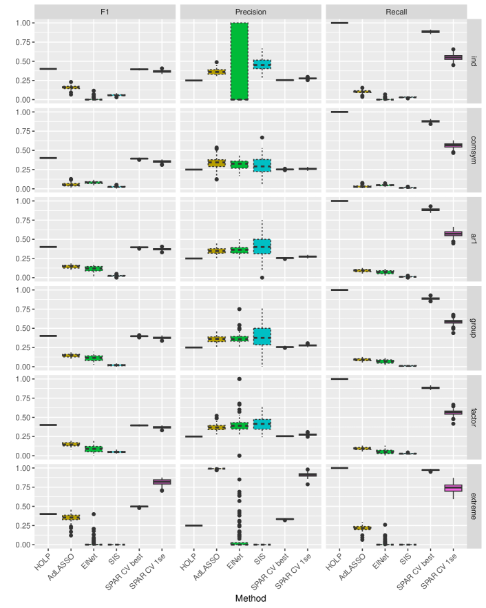
Figure 14: Precision, recall and F1 score of the competing methods, where the sparse methods are marked by dotted boxes, for the six different covariance settings and dense setting for the active variables for $n_{\text{rep}}=100$ replications ($n=200,p=2000,\rho_{\text{snr}}=10$)

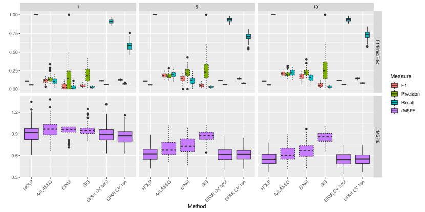
Figure 16: Performance measures of the competing methods, where the sparse methods are marked by dotted boxes, for ’group’ covariance setting, medium setting for the active variables and $\rho_{\text{snr}}=1,5,10$ for $n_{\text{rep}}=100$ replications ($n=200,p=2000$)

Appendix C Gene Selection in Section 4.1

In this section, we look at variable selection for the rateye gene expression dataset from Section 4.1. We consider the six previous methods, as well as selecting the $10$ genes with highest absolute coefficient estimated by ’SPAR 1-se’, called ’SPAR Top10’ in the following. Table 2 shows the ratio of selected genes that were also selected by the other methods (in the columns) for each method (in the rows). We see that there are no big overlaps between the genes selected by the three sparse methods. For example, only $20\%$ of the $30$ genes selected by ElNet are also selected by AdLASSO, and out of the $5$ genes selected by SIS, not a single one is selected by AdLASSO, while $4$ are selected by ElNet. With ’SPAR 1-se’, we also include $46.2\%,30\%$ and $60\%$ of the genes selected by AdLASSO, ElNet and SIS, respectively, and $3$ of the top $10$ genes are also selected by AdLASSO. Since the truth is unknown in this application, it is hard to judge, which variable selection can be trusted the most.

Table 2: Ratios of genes selected by the row method that were also selected by the column method and their estimated number of truly active variables on the full filtered rat eye gene expression dataset with $p=22905,n=120$

	HOLP	AdLASSO	ElNet	SIS	SPAR best	SPAR 1se	SPAR Top10	numAct
HOLP	1.000	0.002	0.001	0.000	0.179	0.058	0.000	22905
AdLASSO	1.000	1.000	0.154	0.000	0.538	0.462	0.077	39
ElNet	1.000	0.200	1.000	0.133	0.367	0.300	0.000	30
SIS	1.000	0.000	0.800	1.000	0.600	0.600	0.000	5
SPAR best	1.000	0.005	0.003	0.001	1.000	0.326	0.002	4107
SPAR 1se	1.000	0.013	0.007	0.002	1.000	1.000	0.007	1337
SPAR Top10	1.000	0.300	0.000	0.000	1.000	1.000	1.000	10

References

- Fan and Lv [2010] Jianqing Fan and Jinchi Lv. A selective overview of variable selection in high dimensional feature space. Statistica Sinica, 20:101–148, 01 2010.
- Wainwright [2019] Martin J. Wainwright. High-Dimensional Statistics: A Non-Asymptotic Viewpoint. Cambridge Series in Statistical and Probabilistic Mathematics. Cambridge University Press, 2019. doi:10.1017/9781108627771.
- Silin and Fan [2022] Igor Silin and Jianqing Fan. Canonical thresholding for nonsparse high-dimensional linear regression. The Annals of Statistics, 50(1):460 – 486, 2022. doi:https://doi.org/10.1214/21-AOS2116. URL https://doi.org/10.1214/21-AOS2116.
- Gruber and Kastner [2023] Luis Gruber and Gregor Kastner. Forecasting macroeconomic data with bayesian vars: Sparse or dense? it depends!, 2023.
- Zou and Hastie [2005] Hui Zou and Trevor Hastie. Regularization and variable selection via the elastic net. Journal of the Royal Statistical Society: Series B (Statistical Methodology), 67(2):301–320, 2005. doi:https://doi.org/10.1111/j.1467-9868.2005.00503.x. URL https://rss.onlinelibrary.wiley.com/doi/abs/10.1111/j.1467-9868.2005.00503.x.
- Zou [2006] Hui Zou. The adaptive lasso and its oracle properties. Journal of the American Statistical Association, 101(476):1418–1429, 2006. doi:https://doi.org/10.1198/016214506000000735. URL https://doi.org/10.1198/016214506000000735.
- Hastie et al. [2009] T. Hastie, R. Tibshirani, and J.H. Friedman. The Elements of Statistical Learning: Data Mining, Inference, and Prediction. Springer series in statistics. Springer, 2009. ISBN 9780387848846. URL https://books.google.at/books?id=eBSgoAEACAAJ.
- Fan and Lv [2007] Jianqing Fan and Jinchi Lv. Sure independence screening for ultra-high dimensional feature space. J Roy Stat Soc, B 70, 01 2007.
- Wang [2009] Hansheng Wang. Forward regression for ultra-high dimensional variable screening. Journal of the American Statistical Association, 104(488):1512–1524, 2009. doi:https://doi.org/10.1198/jasa.2008.tm08516. URL https://doi.org/10.1198/jasa.2008.tm08516.
- Wang and Leng [2015] Xiangyu Wang and Chenlei Leng. High-dimensional ordinary least-squares projection for screening variables. Journal of the Royal Statistical Society: Series B (Statistical Methodology), 78, 06 2015. doi:https://doi.org/10.1111/rssb.12127.
- Clarkson and Woodruff [2013] Kenneth L. Clarkson and David P. Woodruff. Low rank approximation and regression in input sparsity time. In Proceedings of the Forty-Fifth Annual ACM Symposium on Theory of Computing, STOC ’13, page 81–90, New York, NY, USA, 2013. Association for Computing Machinery. ISBN 9781450320290. doi:https://doi.org/10.1145/2488608.2488620. URL https://doi.org/10.1145/2488608.2488620.
- Geppert et al. [2015] Leo N. Geppert, Katja Ickstadt, Alexander Munteanu, Jens Quedenfeld, and Christian Sohler. Random projections for bayesian regression. Statistics and Computing, 27(1):79–101, November 2015. doi:https://doi.org/10.1007/s11222-015-9608-z. URL https://doi.org/10.1007/s11222-015-9608-z.
- Zhou et al. [2007] Shuheng Zhou, Larry Wasserman, and John Lafferty. Compressed regression. In J. Platt, D. Koller, Y. Singer, and S. Roweis, editors, Advances in Neural Information Processing Systems, volume 20. Curran Associates, Inc., 2007. URL https://proceedings.neurips.cc/paper_files/paper/2007/file/0336dcbab05b9d5ad24f4333c7658a0e-Paper.pdf.
- Maillard and Munos [2009] Odalric Maillard and Rémi Munos. Compressed least-squares regression. In Y. Bengio, D. Schuurmans, J. Lafferty, C. Williams, and A. Culotta, editors, Advances in Neural Information Processing Systems, volume 22. Curran Associates, Inc., 2009. URL https://proceedings.neurips.cc/paper_files/paper/2009/file/01882513d5fa7c329e940dda99b12147-Paper.pdf.
- Guhaniyogi and Dunson [2015] Rajarshi Guhaniyogi and David B. Dunson. Bayesian Compressed Regression. Journal of the American Statistical Association, 110(512):1500–1514, 2015. doi:https://doi.org/10.1080/01621459.2014.969425. URL https://doi.org/10.1080/01621459.2014.969425.
- Thanei et al. [2017] Gian-Andrea Thanei, Christina Heinze, and Nicolai Meinshausen. Random Projections for Large-Scale Regression, pages 51–68. Springer International Publishing, Cham, 2017. ISBN 978-3-319-41573-4. doi:https://doi.org/10.1007/978-3-319-41573-4_3. URL https://doi.org/10.1007/978-3-319-41573-4_3.
- Mukhopadhyay and Dunson [2020] Minerva Mukhopadhyay and David B. Dunson. Targeted Random Projection for Prediction From High-Dimensional Features. Journal of the American Statistical Association, 115(532):1998–2010, 2020. doi:https://doi.org/10.1080/01621459.2019.1677240. URL https://doi.org/10.1080/01621459.2019.1677240.
- Kobak et al. [2020] Dmitry Kobak, Jonathan Lomond, and Benoit Sanchez. The optimal ridge penalty for real-world high-dimensional data can be zero or negative due to the implicit ridge regularization. J. Mach. Learn. Res., 21(1), 1 2020. ISSN 1532-4435.
- Wang et al. [2015] Xiangyu Wang, Chenlei Leng, and David B. Dunson. On the consistency theory of high dimensional variable screening. In Proceedings of the 28th International Conference on Neural Information Processing Systems - Volume 2, NIPS’15, page 2431–2439, Cambridge, MA, USA, 2015. MIT Press.
- Zhao and Yu [2006] Peng Zhao and Bin Yu. On model selection consistency of lasso. Journal of Machine Learning Research, 7(90):2541–2563, 2006. URL http://jmlr.org/papers/v7/zhao06a.html.
- Johnson and Lindenstrauss [1984] William Johnson and Joram Lindenstrauss. Extensions of lipschitz maps into a hilbert space. Contemporary Mathematics, 26:189–206, 01 1984. doi:https://doi.org/10.1090/conm/026/737400.
- Frankl and Maehara [1988] P Frankl and H Maehara. The johnson-lindenstrauss lemma and the sphericity of some graphs. Journal of Combinatorial Theory, Series B, 44(3):355–362, 1988. ISSN 0095-8956. doi:https://doi.org/10.1016/0095-8956(88)90043-3. URL https://www.sciencedirect.com/science/article/pii/0095895688900433.
- Achlioptas [2003] Dimitris Achlioptas. Database-friendly random projections: Johnson-lindenstrauss with binary coins. Journal of Computer and System Sciences, 66(4):671–687, 2003. ISSN 0022-0000. doi:https://doi.org/10.1016/S0022-0000(03)00025-4. URL https://www.sciencedirect.com/science/article/pii/S0022000003000254. Special Issue on PODS 2001.
- Li et al. [2006] Ping Li, Trevor J. Hastie, and Kenneth W. Church. Very sparse random projections. In Proceedings of the 12th ACM SIGKDD International Conference on Knowledge Discovery and Data Mining, KDD ’06, page 287–296, New York, NY, USA, 2006. Association for Computing Machinery. ISBN 1595933395. doi:https://doi.org/10.1145/1150402.1150436. URL https://doi.org/10.1145/1150402.1150436.
- Burnham and Anderson [2004] Kenneth P. Burnham and David R. Anderson. Multimodel inference: Understanding aic and bic in model selection. Sociological Methods & Research, 33(2):261–304, 2004. doi:https://doi.org/10.1177/0049124104268644. URL https://doi.org/10.1177/0049124104268644.
- Reeve and Brown [2018] Henry WJ Reeve and Gavin Brown. Diversity and degrees of freedom in regression ensembles. Neurocomputing, 298:55–68, 2018. ISSN 0925-2312. doi:https://doi.org/10.1016/j.neucom.2017.12.066. URL https://www.sciencedirect.com/science/article/pii/S0925231218302133.
- Claeskens et al. [2016] Gerda Claeskens, Jan R. Magnus, Andrey L. Vasnev, and Wendun Wang. The forecast combination puzzle: A simple theoretical explanation. International Journal of Forecasting, 32(3):754–762, 2016. ISSN 0169-2070. doi:https://doi.org/10.1016/j.ijforecast.2015.12.005. URL https://www.sciencedirect.com/science/article/pii/S0169207016000327.
- R Core Team [2022] R Core Team. R: A Language and Environment for Statistical Computing. R Foundation for Statistical Computing, Vienna, Austria, 2022. URL https://www.R-project.org/.
- Friedman et al. [2010] Jerome Friedman, Robert Tibshirani, and Trevor Hastie. Regularization paths for generalized linear models via coordinate descent. Journal of Statistical Software, 33(1):1–22, 2010. doi:https://doi.org/10.18637/jss.v033.i01.
- Saldana and Feng [2018] Diego Franco Saldana and Yang Feng. SIS: An R package for sure independence screening in ultrahigh-dimensional statistical models. Journal of Statistical Software, 83(2):1–25, 2018. doi:https://doi.org/10.18637/jss.v083.i02.
- Scheetz et al. [2006] Todd E. Scheetz, Kwang-Youn A. Kim, Ruth E. Swiderski, Alisdair R. Philp, Terry A. Braun, Kevin L. Knudtson, Anne M. Dorrance, Gerald F. DiBona, Jian Huang, Thomas L. Casavant, Val C. Sheffield, and Edwin M. Stone. Regulation of gene expression in the mammalian eye and its relevance to eye disease. Proceedings of the National Academy of Sciences, 103(39):14429–14434, 2006. doi:https://doi.org/10.1073/pnas.0602562103. URL https://www.pnas.org/doi/abs/10.1073/pnas.0602562103.
- Chiang et al. [2006] Annie P. Chiang, John S. Beck, Hsan-Jan Yen, Marwan K. Tayeh, Todd E. Scheetz, Ruth E. Swiderski, Darryl Y. Nishimura, Terry A. Braun, Kwang-Youn A. Kim, Jian Huang, Khalil Elbedour, Rivka Carmi, Diane C. Slusarski, Thomas L. Casavant, Edwin M. Stone, and Val C. Sheffield. Homozygosity mapping with snp arrays identifies trim32, an e3 ubiquitin ligase, as a bardet-biedl syndrome gene (bbs11). Proceedings of the National Academy of Sciences, 103(16):6287–6292, 2006. doi:https://doi.org/10.1073/pnas.0600158103. URL https://www.pnas.org/doi/abs/10.1073/pnas.0600158103.
- Huang et al. [2006] Jian Huang, Shuangge Ma, and Cun-Hui Zhang. Adaptive lasso for sparse high-dimensional regression. Statistica Sinica, 18, 12 2006.
- Li et al. [2022] Xingguo Li, Tuo Zhao, Lie Wang, Xiaoming Yuan, and Han Liu. flare: Family of Lasso Regression, 2022. URL https://CRAN.R-project.org/package=flare. R package version 1.7.0.1.
- Tenenbaum et al. [2000] Joshua B. Tenenbaum, Vin de Silva, and John C. Langford. A global geometric framework for nonlinear dimensionality reduction. Science, 290(5500):2319–2323, 2000. doi:https://doi.org/10.1126/science.290.5500.2319. URL https://www.science.org/doi/abs/10.1126/science.290.5500.2319.
- Guhaniyogi and Dunson [2016] Rajarshi Guhaniyogi and David B. Dunson. Compressed Gaussian Process for Manifold Regression. Journal of Machine Learning Research, 17(69):1–26, 2016. URL http://jmlr.org/papers/v17/14-230.html.
- Cribari-Neto et al. [2000] Francisco Cribari-Neto, Nancy Lopes Garcia, and Klaus L. P. Vasconcellos. A note on inverse moments of binomial variates. Brazilian Review of Econometrics, 20(2), 2000. URL https://EconPapers.repec.org/RePEc:sbe:breart:v:20:y:2000:i:2:a:2760.