Low latency optical-based mode tracking with machine learning deployed on FPGAs on a tokamak

Abstract

Active feedback control in magnetic confinement fusion devices is desirable to mitigate plasma instabilities and enable robust operation. Optical high-speed cameras provide a powerful, non-invasive diagnostic and can be suitable for these applications. In this study, we process fast camera data, at rates exceeding 100 kfps, on in situ Field Programmable Gate Array (FPGA) hardware to track magnetohydrodynamic (MHD) mode evolution and generate control signals in real-time. Our system utilizes a convolutional neural network (CNN) model which predicts the $n$=1 MHD mode amplitude and phase using camera images with better accuracy than other tested non-deep-learning-based methods. By implementing this model directly within the standard FPGA readout hardware of the high-speed camera diagnostic, our mode tracking system achieves a total trigger-to-output latency of 17.6 $\mu$s and a throughput of up to 120 kfps. This study at the High Beta Tokamak-Extended Pulse (HBT-EP) experiment demonstrates an FPGA-based high-speed camera data acquisition and processing system, enabling application in real-time machine-learning-based tokamak diagnostic and control as well as potential applications in other scientific domains.

I Introduction

High speed optical cameras with intelligent, machine learning (ML)-enabled real-time processing and control capabilities bring entirely new capabilities to a wide-range of scientific applications from cell-sorting to microscopy to fusion Allison McCarn Deiana, Nhan Tran, et al (2022). We present an open-source workflow accessible to domain scientists that embeds a deep learning model in the data acquisition and control loop field programmable gate arrays (FPGAs). We demonstrate this workflow for the application of microsecond-level low latency tracking of magnetohydrodynamic (MHD) instabilites in tokamak plasmas. This system will be used for real-time instability control in upcoming experiments on the High Beta Tokamak-Extended Pulse (HBT-EP) device.

While magnetic confinement devices can be designed to operate far from stability limits with nominal plasma conditions, transient events or other deviations from desired parameters may lead to instability. Efficient usage of the applied magnetic field to confine higher plasma pressure generally leads to less stable equilibria due to $\beta$-driven instabilities (with $\beta=\frac{\mathrm{nT}}{\mathrm{B}^{2}/2\mu_{0}}$). As tokamaks and other magnetic confinement devices achieve fusion-relevant conditions, real-time diagnosis and control of plasma instabilities is essential for maintaining desirable plasma parameters and robust performance. Plasma conditions and instabilities in tokamaks can evolve on an Alfvénic timescale for the most demanding cases, necessitating fast evaluations and control decisions on a timescale of microseconds for quickly growing or rotating kink and tearing instabilities Chu and Okabayashi (2010). For this reason, real-time control of plasma properties requires reasonably accurate implementation of control algorithms with latencies commensurate with the plasma dynamics.

Recently, deep learning LeCun, Bengio, and Hinton (2015) and other data-driven machine learning techniques have been applied to a variety of areas in plasma and fusion research. For tokamak control applications, current studies have mainly focused on the prediction and control of disruptive events and equilibrium quantities. These studies can be broadly divided into two categories: 1. by developing a data-driven model to predict the intended plasma quantities Jalalvand et al. (2022); Boyer and Chadwick (2021); Zhu et al. (2023); Kates-Harbeck, Svyatkovskiy, and Tang (2019) and using these predictions to inform a non-machine-learning-based control algorithm Abbate et al. (2023); Wei et al. (2021), or 2. by training a deep reinforcement learning agent on a computational Degrave et al. (2022); Dubbioso et al. (2023) or data-driven Seo et al. (2022); Char et al. (2023) simulator and using the trained agent to directly generate control policies. Some of these trained models have also been tested in real-time and have achieved latencies on the order of the device’s PCS cycle time, ranging from milliseconds to as low as 50 $\mu$s Abbate et al. (2023); Boyer and Chadwick (2021); Shin et al. (2022); Char et al. (2023); Degrave et al. (2022).

Besides disruption and equilibrium, prediction and control of non-equilibrium quantities such as MHD instabilities Piccione et al. (2022); Wei et al. (2023) and ELMs Shin et al. (2022); Song et al. (2023) using machine learning approaches have also been investigated. However, applying these models for real-time control can be more challenging as the model needs to perform inference with latency similar to or smaller than the timescale of the plasma event which can be as fast as in the microsecond or nanosecond range. Depending on the complexity of the specific algorithm, a real-time implementation may require special optimization and computing hardware in order to achieve the target latency.

In this paper, we present one of the first real-time low-latency applications of a deep learning algorithm for MHD mode control on a tokamak device. Continuing our previous study on combining high-speed imaging camera diagnostics and convolutional neural networks (CNNs) for tracking $n$=1 long wavelength MHD modes on the HBT-EP experiment Wei et al. (2023), we further developed and implemented our CNN model on an FPGA device onboard the Euresys frame grabber card in the existing camera diagnostic system. FPGA-based computing platforms have enabled neural network models to perform online single-sample inference with latencies in the 100 ns to 10 $\mu$s range Aarrestad et al. (2021), far outperforming their counterpart GPU implementations. However, deploying a model on an FPGA device presents several challenges, including designing within the resource constraints of the FPGA chip. For this reason we utilized the High-Level Synthesis for Machine Learning (hls4ml) FastML (2023) package to optimize our model before synthesizing and deploying the model firmware to the frame grabber’s FPGA. Our implementation achieved a latency of 7.7 $\mu$s for the CNN model itself, 17.6 $\mu$s total for the acquisition trigger to output control request, and is capable of operating at pipelined frame rates of up to 120 kfps, satisfying the requirement for MHD mode control on HBT-EP. This is the first demonstration of 100 kHz low-latency control algorithms for real-time MHD mode tracking using raw high-speed camera outputs in fusion experiments.

The layout of this paper is as follows. In Section II, we describe the HBT-EP Tokamak experiment and the fast camera system used for MHD mode tracking. We detail the choice of readout technology used for implementing the control algorithm in real time and the tools we use for deploying machine learning algorithms in FPGA readout hardware. In Section III, we describe the deep learning algorithm optimization for the fast camera readout hardware and the performance of the algorithm. This includes trade-offs between computing resources, latency, and performance. Then, in Section IV we detail the final implementation and validation of the control algorithm deployed at the HBT-EP experiment. Finally, we summarize and describe future work.

II System design

II.1 Diagnostics and hardware

HBT-EP Maurer et al. (2011) is a circular, ohmically heated, large aspect ratio tokamak (R/a $\sim$ 6). It has an on-axis toroidal magnetic field of 0.33 T, typical plasma currents of 15 kA, a major radius of 0.92 m, and a plasma minor radius of 0.15 m. Figure 1 shows the HBT-EP high-speed camera diagnostic setup. The setup consists of two Phantom S710 cameras which are capable of operating at frame rates between 100-400 kfps. The cameras are placed away from the toroidal field (TF) coils and measure visible light emissions, predominantly of the D-alpha line from the plasma edge Angelini et al. (2015), through a midplane glass viewing port using a fiber bundle and relay lenses. This system offers high flexibility and has been used to study MHD activities during the “flat-top” period Angelini et al. (2015) or during disruptions Saperstein (2023) through the use of different camera views, frame rates, and exposure settings.

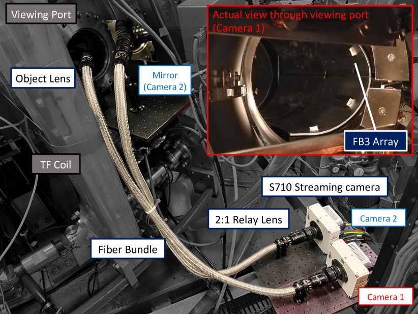
Figure 1: Hardware setup of the high-speed camera diagnostics on HBT-EP as used during the previous run campaign Wei et al. (2023), with an actual view of the chamber (similar to Camera 1 view) shown in the top-right inset. The same database was used in this study for training and testing the various CNN models for FPGA implementation as described in the following sections. Reused with permission from Y. Wei et al (2023) PPCF 65 074002. Copyright 2023 IOP Publishing.

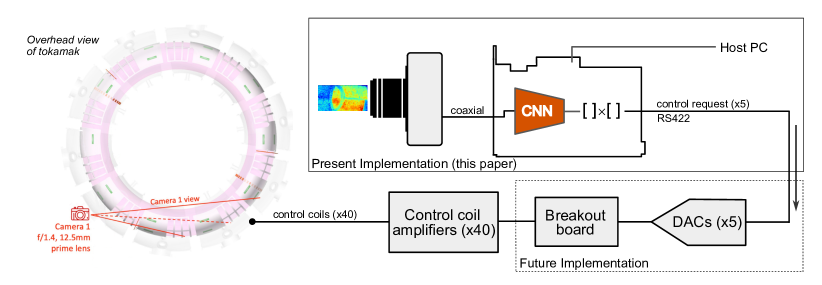
Figure 2: Data flow in the proposed camera-and-FPGA-based active feedback control system.

The Phantom S710 does not possess the capability to process the camera sensor readout; instead, a dedicated PCIe frame grabber card is required to capture and interpret the raw camera data into monochrome images. We use a Euresys Coaxlink Octo frame grabber card which utilizes the CoaXPress camera interface standard and implements its image processing capabilities on a Xilinx Kintex UltraScale KU035 FPGA. Euresys enables the user to also implement custom firmware on the card’s FPGA through a reference design toolkit called CustomLogic Euresys (2021a). For this project, we leveraged this toolkit to implement our CNN on the frame grabber’s FPGA and subsequently write the computed control request over the frame grabber’s RS422 I/O pins. In placing the computation and output request generation on the acquisition card, we avoid the overhead associated with multiple PCIe hops, latency associated with standard processors, and the cost associated with developing a highly-custom solution. Currently, CustomLogic only supports the use of a single frame grabber card and one of the two available CXP-6 connection banks on the Coaxlink Octo card. This restricts us to using only one of the two available cameras in this real-time system and limits the maximum achievable frame rate compared to the passive diagnostic setup.

Figure 2 shows the data flow of the proposed camera-based control system on HBT-EP. We use a single camera (Camera 1) which captures a cross-sectional view of the plasma. The captured frames are streamed in real time to the frame grabber card, which processes the optical data, passes the images through the neural network model and generates new control requests. Currently, we measure these output control requests and other auxiliary signals on an oscilloscope to verify the timing and latency of the system. In the future control system, these control requests will be sent to multiple digital-to-analog converters (DACs) which will be connected to the existing amplifiers to generate the target mode shape on the radial field saddle control coils. This DAC and breakout board system is presently being designed and will be assembled and tested in the near future.

II.2 Design considerations

The proposed real-time control system is subject to two major design constraints: the system latency and the available FPGA resources.

Firstly, MHD modes on HBT-EP typically rotate at frequencies around 10 kHz which corresponds to a period of 100 $\mu$s. In order to suppress these modes, the control system needs to achieve a total input-to-out latency several times smaller than a rotation period and a sampling interval (i.e., the initiation interval, the frequency at which the system can process a new input) at a similar level, if not faster. Currently, the fastest implementation of the GPU-based control system on HBT-EP has achieved latencies around 16 $\mu$s and sampling intervals between 4–6 $\mu$s Rath et al. (2013); Peng et al. (2016). This system, however, is significantly less computationally challenging compared to our proposed setup as it takes in one or two orders of magnitude less input data with 40–80 magnetic sensor channels compared to 1,024–8,192 pixels (depending on the actual image resolutions) and uses a single matrix multiplication as opposed to a neural network to perform mode tracking. These distinctions make achieving similar levels of latency and sampling intervals considerably more challenging for a high-speed camera and FPGA-based control system and have been our primary considerations during our design and optimization phases.

Secondly, the total resource capacity of our frame grabber card’s FPGA is relatively small compared to modern FPGA-based data center and accelerator cards used in high-throughput applications. This FPGA consists of just over 200,000 look-up tables (LUTs) and 1,700 digital signal processing (DSP) blocks, the two elements primarily used for matrix-vector multiplication arithmetic and logic, and 540 block RAMs (BRAMs). In addition, approximately 25% of the LUTs, 10% of the DSPs, and 35% of the BRAM resources are dedicated to implementing the CoaXPress protocol and other proprietary frame grabber firmware, which further restricts our model size and potential for latency optimization.

Given these two major constraints, our goal in terms of the hardware co-design is to find a solution that achieves an optimal trade-off between the model’s prediction performance and its latency while fitting within the resource constraints of the frame grabber FPGA. The model optimization and synthesis process using hls4ml is described in the following section.

III Neural network model co-design

III.1 Training dataset

The CNN models are developed using a dataset collected from a previous run campaign Wei et al. (2023). This dataset consists of camera frame images and the corresponding magnetic mode signals at 86,275 time slices (or samples) over 45 discharges. These shots used a mode-control-type shot style on HBT-EP and contained both $m/n$ = 4/1 and 3/1 modes (where $m$ and $n$ are the poloidal and toroidal mode numbers respectively) rotating at around 8–12 kHz during different time periods of the the discharge. We divided the dataset the same way as in the previous study, by using the first 40 shots as the training set (76,975 samples) and the last 5 shots as the testing set (9,300 samples). The training set is further split randomly by samples using a 9:1 ratio into training and validation for hyperparameters tuning.

The frame images were captured by the two Phantom S710 cameras through an optical view port (Figure 1). Both cameras had a cross-sectional view of the plasma toward opposite toroidal directions. The images were taken at 250 kfps, 128$\times$64 pixels (width$\times$height) resolution, 12-bit grayscale bit depth, and 3 $\mu$s exposure time. For this study we only used the images from Camera 1 to train the CNN models due to the present constraint of CustomLogic, although it has been shown that using images from both cameras slightly improved the accuracy of the model’s predictions Wei et al. (2023).

For the ground truths (or training labels), we used the sine and cosine components of the $n=1$ mode determined from an in-vessel low-field-side magnetic sensor array (FB3). This sensor array has been used extensively during previous mode control experiments and for evaluating other non-magnetic mode tracking methods, therefore by accurately reproducing these signals the camera-based mode tracking system should achieve similar mode suppression results. In future iterations of this system, the ground truth information may be acquired from alternative diagnostic or numerical source that requires extensive post-shot analysis in order to better leverage the strengths of CNNs for image regression and low-latency inference through FPGAs.

III.2 Model optimization strategy

We implemented the CNN model in the readout path of Camera 1 in the Euresys Coaxlink Octo frame grabber card, and utilized the hls4ml package to compile the model, originally implemented in Tensorflow Abadi et al. (2015), into a high-level synthesis (HLS) representation. This compiled HLS model is then synthesized to a register-transfer level (RTL) description using the Xilinx Vivado Design Suite Xilinx (2018) and subsequently deployed to the target FPGA device.

To tailor our CNN model for the previously mentioned HBT-EP system constraints, hls4ml offers a variety of optimizations to meet hardware resource and latency requirements. Efficient model design for hardware is a multi-dimensional design space from CNN hyperparameter choices to hardware microarchitecture implementation. On the hardware implementation side, there are three primary high-level optimizations available to the user in hls4ml. First, using full 32-bit floating point input data and parameter representation for the model in hardware is unnecessary. Therefore, hls4ml utilizes arbitrary-precision fixed-point representations more suited for FPGA hardware to store model weights and activations. The user can take advantage of post-training quantization (PTQ) to appropriately select the weight and accumulator bit widths after training the model. More optimally, the user can account for quantization during training using quantization-aware training (QAT) frameworks like QKeras Google (2020), Brevitas Pappalardo (2023), and HAWQ Dong et al. (2019). In this study, we use the QKeras framework, built on Keras Chollet et al. (2015), and TensorFlow for customizable quantization. QAT often yields more optimally (lower precision) trained neural networks over PTQ.

In addition to quantizing the parameters, the model’s resource usage can be reduced further by applying sparsity to its weights and biases. This can be done using tools like the Pruning API in the TensorFlow Model Optimization Toolkit Google (2023) to arbitrarily force a certain percentage of the parameters to be zero during training. hls4ml can account for these zero parameters during it’s conversion process, thus reducing the number of parameters needed to implement each of the pruned layers.

Finally, hls4ml leverages the highly parallel architecture of the FPGA fabric through a “reuse factor” tunable parameter (i.e. how many times a logic element is reused during one inference). This option grants the user direct control over the degree of parallelization of the multiply-accumulate operations on a per-layer basis, enabling fine control over latency-area optimization. Additionally, dataflow pipelining enables further parallelization at the functional layer level, significantly reducing overall latency to nearly match the highest consumer. We utilize this set of features, along with our own HLS and hardware optimizations outlined below to implement our CNN under challenging area and latency constraints.

III.3 Selected candidate models

Using these optimization techniques with the Tensorflow, QKeras, and hls4ml tool flows, we leverage the co-design process to select a candidate model for implementation. All of these models share a similar network architecture to the single-camera single-frame model as described in Ref. 16, in using three Conv2D-MaxPool layers followed by two hidden dense layers and the output layer. We describe each of these representative candidate models below. The relevant metrics for these models are compared in Table 1.

Model Name	PPCF23	QAT+Pruning	Optimized
Image Resolution	128$\times$64	128$\times$64	32$\times$32
Conv Layer Filters	{8, 8, 16}	{8, 8, 16}	{16, 16, 24}
Dense Layer Widths	{256, 64}	{256, 64}	{42, 64}
Total Parameters	362,730	362,730	12,910
Parameter Precision	PTQ, 18 bits	QAT, 8 bits	QAT, 7 bits
Sparsity	none	80%	50%
Bit Operations	3.62e13	6.86e12	2.85e11
Reuse Factors	[1, 1, 1, 168, 8, 1]	[1, 4, 16, 48, 64, 128]	[1, 4, 16, 48, 64, 128]

Table 1: Comparison of hyperparameters and configurations for the PPCF23 (baseline), QAT+Pruning, and Optimized models described in Section III.3. Reuse factors selected for each layer of the networks are shown in the order: conv0, conv1, conv2, dense0, dense1, dense2. A lower value indicates a higher level of parallelization.

• The baseline implementation is called PPCF23 after Ref. 16 and uses the training hyperparameters from the original single-camera single-frame model. We applied minimal modifications to this implementation by only scanning the model and layer bit widths through PTQ to maintain performance with respect to the original 32-bit floating point model.

• QAT+Pruning: A modified implementation based on the original model. For this model we applied QAT by replacing the Conv2D, ReLU, and hidden Dense layers with the corresponding quantized layer from the QKeras library. We scanned the quantization levels and sparsity using the training and validation sets; after determining the optimal hyperparameters, we trained the model one more time using the entire training dataset to obtain the final model parameters.

• Optimized: A compressed and optimized implementation. This model uses a smaller input resolution of $32\times 32$ as opposed to $128\times 64$ used in all previous models, as well as fewer neurons at the first fully connected layer. The number of filters in the three QConv2D layers were also increased from [8, 8, 16] to [16, 16, 24] respectively which from our tests were shown to improve the model’s accuracy, potentially due to increased data flow into the downstream dense layers. These measures significantly reduced the number of model parameters by more than 96%, not accounting for sparsity.

The list above does not outline all tested neural network models, but rather represents the most important optimizations that were performed in this study during the design space exploration. The other crucial optimization on the hardware side we performed was determining a reasonable level of parallelization for each layer of the network through hls4ml’s reuse factor parameter. Fine-tuning these reuse factors can reduce FPGA resource usage while maintaining a sufficiently low model latency.

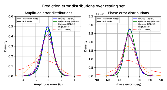
Figure 3: Distributions of the amplitude (left) and phase (right) prediction errors over the testing set (ground truth amplitude $>$3G), given by the three candidate CNN models. For each model the results of the Tensorflow implementation are shown in solid lines, and that of the converted HLS implementation are shown in dashed lines. Results of two additional non-deep-learning-based methods using linear regression and SVD-based algorithms Wei et al. (2023) are included for comparison. All models except the Optimized model use input images of $128\times 64$ pixels resolution, whereas the Optimized model uses $32\times 32$ pixels resolution.

The first two implementations (PPCF23 and QAT+Pruning) failed to achieve the targeted latency and resource criteria (see Table 2 and more discussion in Section III.4). We have attempted to further adjust the hyperparameters of the QAT+Pruning model but did not arrive at a solution that satisfies our constraints. This was the primary reason why we decided to reduce the input dimensions in the Optimized implementation which significantly reduced the overall number of bit operations. We then adjusted the layer hyperparameters to maintain the overall performance as described previously. These resulted in a slightly reduction in the model’s prediction accuracy compared to the previous two models but significantly improved the hardware resource usage and latency.

III.4 Model performance and implementation results

Figure 3 compares the amplitude and phase error distributions of the predictions given by these three models; the results of the simpler, non-deep-learning, linear regression model and SVD-based models from the previous study Wei et al. (2023) are also included for references. These distributions are obtained using data from the five test discharges during the mode active periods (ground truth amplitude $>$3G) in accordance with our previous analysis method. For each of the three CNN models, both the results of their original Tensorflow implementation (solid lines) and those of the converted hls4ml implementation (dashed lines) are shown in these figures. We observed slight degradation in model accuracy after this conversion step especially for the amplitude predictions.

Among the three CNN models, the results of the second model (green lines) effectively matched those of the original model (solid blue lines) from the previous study even after the conversion (dashed green lines). This demonstrates the effects of applying QAT and sparsity on a neural network, as the now-compressed model maintains its prediction accuracy despite having 80% of its network parameters set to zero while the remaining parameters using 24 fewer bits than those of the full Tensorflow model. However, given the especially tight constraints of this specific project, we compromised in using the third model (purple lines), which performs slightly worse than the two previous models but still yields a large improvement over the two non-neural-network-based algorithms.

A comparison of single-shot tracking performances using the three models after hls4ml conversion is shown in Figure 4. All three models are able to track both the amplitude and phase evolution across the entire discharge with reasonable accuracy. The phase predictions are only inaccurate when the mode amplitude was very small, such as at 6 and 8.4 ms in this shot. A slightly higher level of fluctuation is observed for the Optimized model in both its amplitude and phase predictions compared to the other two models. At this moment we do not believe this would affect the actual field applied to the plasma as these high frequency fluctuations would be “smoothed out" by the control coil amplifiers and therefore should not affect the outcome in a control experiment; the exact effect will be investigated in the following study.

Figure 4: Comparison of single shot tracking performance of the three candidate models after hls4ml conversion, using testing shot 114467. The 4/1 and 3/1-dominant periods are highlighted in cyan and yellow respectively. Top: Amplitude (left) and phase (right) ground truth calculated from magnetic sensors. Bottom 3 rows: Amplitude (left) and phase (right) prediction errors of the candidate models.

Using the Optimized model, we further optimized the hardware implementation by tuning the reuse factor of the model. Figure 5 shows the latency vs. FPGA resource usages of implementations using different reuse factors. We observe a trade-off between resource usages and computational latency as we increase the reuse factor. Through this approach, we select the proper reuse factor for each of the neural network layers to fit within the resource limits while keeping the latency as low as possible.

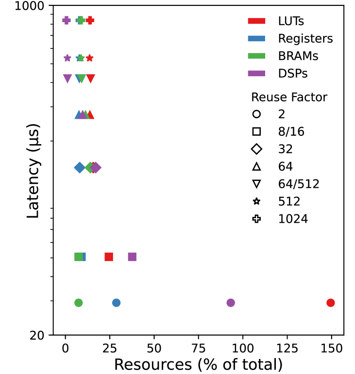
Figure 5: Pareto frontier of optimized model’s resource-latency configurations with increasing levels of parallelization. Colors represent the types of resources available on an FPGA: LUTs, Registers, BRAMs, and DSPs. Shapes represent different reuse factors. Resource usages are shown as % of available resources on the KU035 FPGA. The final optimized model uses different reuse factors for different layers (see Table 1)

The estimated latencies, initiation intervals, and resource usages for this Optimized model and for the implementations of the two other models are shown in Table 2. These estimate reflects only neural network logic usage and excludes the camera protocol and other logic. The implementation of the Optimized model achieved both our latency and resource targets. In particular, the estimated latency of 6.6 $\mu$s is significantly lower than our target total latency of 16 $\mu$s, leaving a large margin for other processes such as image exposure, readout, and control request generation for integration with the control loop. The procedure for integrating this model with the frame grabber firmware is described in the next section.

Model	Latency ($\mu s$)	Interval ($\mu s$)	BRAM	DSP48	Register	LUT
PPCF23	64.3	42.4	21.5%	100.0%	96.7%	828.3%
QAT+Pruning	65.6	42.9	17.9%	100.0%	84.0%	399.9%
Optimized	6.6	5.2	9.3%	7.8%	10.9%	36.7%

Table 2: Comparison of latency and resource usage estimates from logic syntheses for the three candidate models. Resource usage estimates are shown as percentage of the respective type of resource available on the KU035 FPGA.

IV Hardware implementation

IV.1 Firmware integration

After compiling the optimized model to HLS representation, we integrated the neural network IP (intellectual property) block into the larger system firmware infrastructure and readout chain. Figure 6 shows the firmware block diagram of the Euresys Coaxlink Octo frame grabber. Image data transmitted over the CoaXPress interface enters the diagram through the CoaXPress CXP-6 connectors (green, upper left). The pixel data is then buffered before moving to the pixel pre-processing block and then streamed to the CustomLogic block where we integrate our synthesized hls4ml neural network block. The output (and input image) can then be retrieved on the host computer over PCIe and over the general purpose I/O pins.

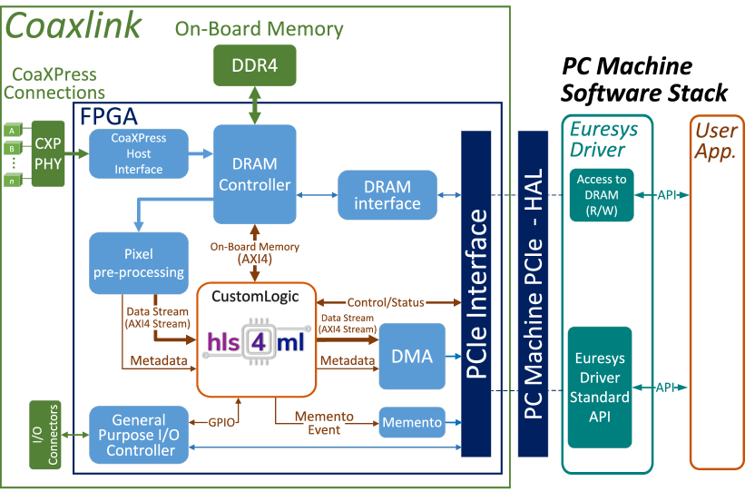
Figure 6: Euresys CustomLogic framework block diagram. Figure adapted from Reference Euresys, 2021b.

To integrate the neural network into the reference design, we leverage HLS to create the appropriate top level ports using properly sized input data types, implemented with an AXI-stream interface ARM (2010). To ensure we extract and provide the correct data to the model, we track the current frame line and pixel position relative to the data stream using positional metadata provided with each data packet. Our current design duplicates the data stream, forwarding the original image to the PCIe interface and the duplicate to the model input. As a result, model inference continues in parallel with uninterrupted frame acquisition. Each data packet comprising the image contains eight pixels which divides the total time to input the image to the network by a factor of eight.

We note a number of design challenges encountered when integrating our model. Generally, meeting the camera protocol’s timing constraint of 250 MHz was a challenge which we overcame with physical optimization tools and hyperparameter searches of the best synthesis strategies. Additionally, the ordering of the image lines within the data stream from the CoaXPress protocol IP do not match the natural (top-left to bottom-right) order of the captured image, but is instead divided into “stripes” (see Figure 7). Since our neural network expects a naturally ordered input, and since first-in first-out (FIFO) memories are not addressable, we implement a stream reordering operation using intermediate FIFOs to store the split input stream before they are emptied in natural order. Furthermore, since the camera resolution has a minimum of $128\times 32$, we track and pass only data packets belonging to the center $32\times 32$ region of interest to the model input.

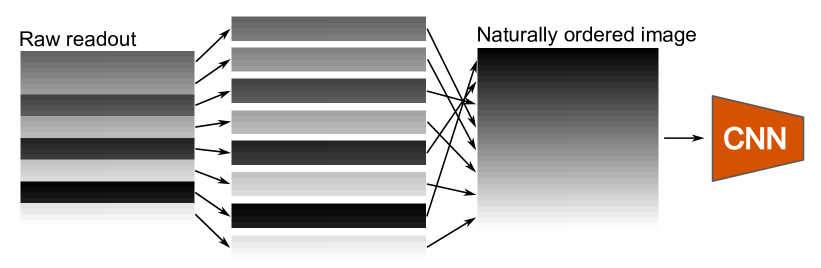
Figure 7: Pixel stream reordering operation implemented in the FPGA firmware.

Control system outputs:

We then implement the control request output of the frame grabber with an ap_vld interface. These control requests are calculated in the firmware through a single matrix multiplication using:

$$v_{i,t}=g[s_{t}sin(m\theta_{i}+n\phi_{i}+\gamma)+c_{t}cos(m\theta_{i}+n\phi_{i}+\gamma)]$$ (1)

where $s_{t}$, $c_{t}$ are the sine and cosine components of the $n$=1 mode predicted by the neural network model, $\theta_{i}$ and $\phi_{i}$ are the poloidal and toroidal locations of control coil, $m$, and $n$ are the mode shape we intend to control, and $g$ and $\gamma$ are the gain and phase shift parameters to be scanned during a feedback control run campaign Peng et al. (2016). In the current implementation, the gain and phase shift factors are set to fixed values; for future versions of the firmware we would need the ability to adjust these values quickly between two consecutive discharges

The control coils on HBT-EP are grouped into four toroidal arrays, each consisting of ten coils spaced evenly in the toroidal direction. These four arrays are independent, but can also be hardwired to create phase shifts to generate arbitrary poloidal mode shape between $m$=1–4. Since we are targeting the $n$=1 mode, we can significantly simplify the problem by outputting only 5 control requests for half of one toroidal array (5 neighboring coils in one array) and mapping these five signals to all 40 coils using a breakout board to generate the desired mode shape. Note that this setup would only work when applying feedback control to a single $m/n$ mode. Multi-mode control tasks would require either switching the mode shape in the middle of a shot, or generating the requests through alternative methods. These will be explored in future studies on HBT-EP.

After computing the control requests, we map their decimal representations to a 12-bit unsigned range and transmit each request serially over 5 pairs of RS422 differential output ports on the frame grabber board which are capable of speed up to 10 MHz. The frame grabber will also supply the necessary serial clock and chip select control signals which are required for the DAC chip we will use for the future system. An additional on/off signal is mapped to an output port to indicate the beginning and conclusion of model inference. This allows us to empirically measure inference latency using an oscilloscope (see Figure 9 (bottom)).

Validation and verification:

For this work, we also developed a C testbench which logs the model output, input cropping and reordering, control request generation, and unsigned request mapping, allowing us to rapidly test and verify the HLS design. However, while this tool enables verification of the algorithms implemented in HLS prior to synthesis, we must also validate the results in hardware.

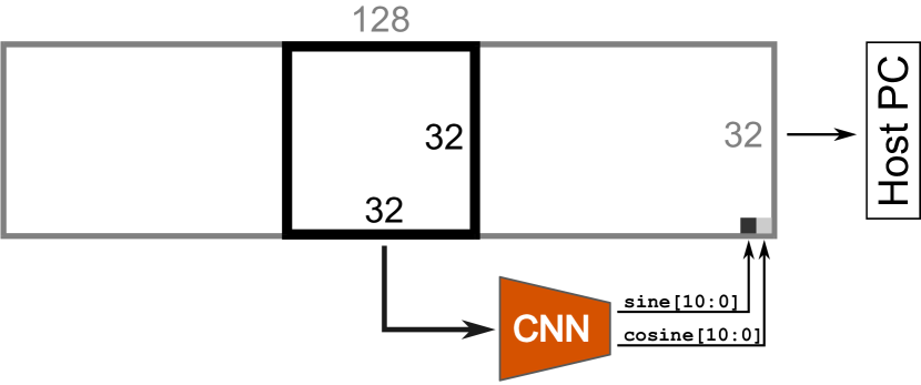
Figure 8: Method for model validation. The outputs of the firmware model are embedded to the lower right region of the captured $128\times 32$ pixels resolution image, outside the actual $32\times 32$ pixels region used by the implemented CNN model. This image is subsequently transferred over PCIe to the host-PC where the embedded predictions are compared with that of the same model running in a Python environment.

Translating and verifying model results with its software counterpart using a bitwise writeout is time-consuming. Instead, we developed a significantly more scalable solution to validate the accuracy of our models across seconds’ worth of image acquisition. As our model considers only the center 32x32 crop of the full 128x32 acquisition, we have designed a variant of our firmware that embeds the model predictions into the outer region of the image (see Figure 8). These modified images which carry their corresponding model predictions are then transferred over PCIe to the host computer’s memory. This approach enables us to validate the firmware accuracy over large amounts of data using a simple Python script. This output embedding is removed in the final firmware version to reduce latency and resource usage. The implementation does not require modifications to the eGrabber API to retrieve the model predictions, which is left for future efforts.

IV.2 System-level results

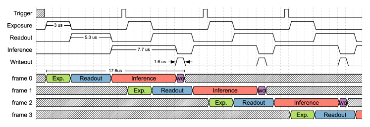
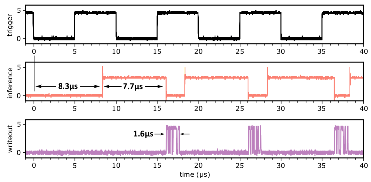
Figure 9: Frame grabber process timing diagram – Top: Acquisition timing diagram at 100 kfps illustrating pipelined image capture and inference. “Exp.” denotes camera exposure, and “wo” denotes serial writout operation. Bottom: Oscilloscope latency measurement on the prototype platform at 100 kfps validating the timing diagram

The final resource consumption breakdown for the final implementation on the frame grabber FPGA (post-placement and routing) is shown in Figures 10. The resource usages are divided into three categories: the neural network model (includes cropping logic and control request calculation), the CoaXPress protocol logic, and other miscellaneous components. The neural network resource consumption is broken down further by layer and an additional “other” category which accounts for components such as BRAM-based FIFO data streams (these constitute the model input and the channels to transport activations from one layer to the next). Among the neural network layers, the convolutional layers require the most logic separate from multiply-accumulates, and therefore use the highest percentage of LUTs. The dense layers possess the highest parameter count, and therefore use the highest percentage of BRAMs for weight storage.

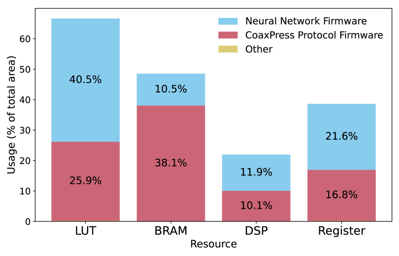
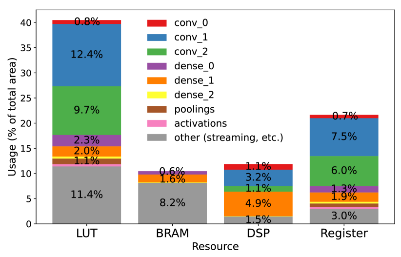
Figure 10: Frame grabber FPGA resource breakdown – Top: overall IP core usage and breakdown between CoaxPress protocol and neural network. Bottom: Resource usage breakdown within the neural network IP across the model architecture.

We deployed the final firmware on the frame grabber card and measured the total latency of the system on an oscilloscope. Figure 9 (bottom) shows the oscilloscope measurements over a period of four frames at 100 kfps beginning with a camera capture trigger and ending with the final control output; an equivalent timing diagram is shown in figure 9 (top). This system achieves a trigger-to-output latency of 17.6 $\mu$s, in which the 3 $\mu$s are attributed to camera exposure, 5.3 $\mu$s to camera readout and DRAM buffering, 7.7 $\mu$s to model inference, and finally 1.6 $\mu$s to serial writeout operation. Through pipelining model inference with the exposure and readout processes, we achieve throughputs of up to 120 kfps which corresponds to a minimum sampling interval of 8.3 $\mu$s. These results satisfy the latency and sampling interval requirements for performing real-time feedback control on HBT-EP and are only slightly slower compared to the previous GPU-based system Rath et al. (2013); Peng et al. (2016).

V Discussion and future work

In this study, we have demonstrated an end-to-end workflow for implementing a deep learning model on an FPGA device for tracking the $n$=1 MHD mode evolution using high-speed camera data. Our system achieves a total latency of 17.6 $\mu$s in which 7.7 $\mu$s is attributed to CNN model inference. Through pipelined operation, our system is capable to operate at up to 120 kfps. These satisfy the requirements for performing real-time feedback control of the $n$=1 MHD mode on HBT-EP. This is also the first demonstration of high-throughput microsecond-level low-latency implementation of a deep learning model for real-time diagnostic and control for plasma and fusion application.

The demonstrated workflow involves optimizing the CNN model in consideration with the available resources in the KU035 FPGA onboard the Euresys Coaxlink Octo frame grabber card. We used the open-source hls4ml package and optimization techniques including hyperparemeter optimization, quantization, pruning, and parallelization through setting reuse factors. This co-design process allowed us to meet both the system latency and FPGA resource requirements.

Final integration and demonstration of the camera-and-FPGA-based real-time feedback control system requires addressing a few remaining points. To close the control loop requires an additional but simple DACs (digital-to-analog converters) and breakout board system (Figure 2) to interface with the camera and frame grabber card implemented in this study with the downstream control coil actuators on HBT-EP. This additional system will take in the 5 control requests generated by the frame grabber card and map them to 40 coil voltage signals to generate a pre-selected mode shape. This is currently being designed and will be tested in the near future. In addition, recent machine and diagnostic upgrades have changed the boundary conditions of HBT-EP plasma and thus making the current data set and model obsolete for the current plasma. For this reason, additional training data needs to be collected for updating the neural network parameters in the FGPA firmware prior to the control experiments. This, however, should not affect the performance of the FPGA-based mode tracking system in terms of latency, throughput, and system design and resources.

The last point on model retraining and adaptability to changing conditions is of particular interest for future studies. The attraction of machine learning is to be able to adapt the algorithm for system needs and continuous running. The current algorithm is effectively performing a regression task to extract the MHD mode signals of the plasma. However, there are a number of novel directions for real-time control such as extending the platform for continuous monitoring and active learning, including domain adaptation or robustness methods in the model training, or changing the paradigm from supervised learning, which requires truth information of magnetic sensors, to real-time reinforcement learning which learns directly from the running system or in a simulator environment. Our study opens these possibilities at the fastest speeds and the natural timescales of the most challenging plasma dynamics.

Finally, the real-time camera-and-deep-learning-based diagnostic system demonstrated in this study could have many applications beyond plasma and fusion research. This system takes off-the-shelf camera and frame grabber components, uses standard data streaming protocols, and applies open-source packages and workflows for optimizing and deploying a neural network model in situ. We believe this platform brings new scientific instrumentation capabilities to a wide range of application domains and is accessible to a wide audience.

References

- Allison McCarn Deiana, Nhan Tran, et al (2022) Allison McCarn Deiana, Nhan Tran, et al, Frontiers in Big Data 5 (2022), 10.3389/fdata.2022.787421.
- Chu and Okabayashi (2010) M. S. Chu and M. Okabayashi, Plasma Physics and Controlled Fusion 52, 123001 (2010).
- LeCun, Bengio, and Hinton (2015) Y. LeCun, Y. Bengio, and G. Hinton, Nature (London) 521, 436 (2015).
- Jalalvand et al. (2022) A. Jalalvand, J. Abbate, R. Conlin, G. Verdoolaege, and E. Kolemen, IEEE Transactions on Neural Networks and Learning Systems 33, 2630 (2022).
- Boyer and Chadwick (2021) M. Boyer and J. Chadwick, Nuclear Fusion 61, 046024 (2021).
- Zhu et al. (2023) J. Zhu, C. Rea, R. Granetz, E. Marmar, R. Sweeney, K. Montes, and R. Tinguely, Nuclear Fusion 63, 046009 (2023).
- Kates-Harbeck, Svyatkovskiy, and Tang (2019) J. Kates-Harbeck, A. Svyatkovskiy, and W. Tang, Nature (London) 568, 526 (2019).
- Abbate et al. (2023) J. Abbate, R. Conlin, R. Shousha, K. Erickson, and E. Kolemen, Journal of Plasma Physics 89, 895890102 (2023).
- Wei et al. (2021) Y. Wei, J. P. Levesque, C. J. Hansen, M. E. Mauel, and G. A. Navratil, Nuclear Fusion 61, 126063 (2021).
- Degrave et al. (2022) J. Degrave, F. Felici, J. Buchli, M. Neunert, B. Tracey, F. Carpanese, T. Ewalds, R. Hafner, A. Abdolmaleki, D. de las Casas, C. Donner, L. Fritz, C. Galperti, A. Huber, J. Keeling, M. Tsimpoukelli, J. Kay, A. Merle, J.-M. Moret, S. Noury, F. Pesamosca, D. Pfau, O. Sauter, C. Sommariva, S. Coda, B. Duval, A. Fasoli, P. Kohli, K. Kavukcuoglu, D. Hassabis, and M. Riedmiller, Nature (London) 602, 414 (2022).
- Dubbioso et al. (2023) S. Dubbioso, G. De Tommasi, A. Mele, G. Tartaglione, M. Ariola, and A. Pironti, Fusion Engineering and Design 194, 113725 (2023).
- Seo et al. (2022) J. Seo, Y. S. Na, B. Kim, C. Y. Lee, M. S. Park, S. J. Park, and Y. H. Lee, Nuclear Fusion 62, 086049 (2022).
- Char et al. (2023) I. Char, J. Abbate, L. Bardoczi, M. Boyer, Y. Chung, R. Conlin, K. Erickson, V. Mehta, N. Richner, E. Kolemen, and J. Schneider, in Proceedings of The 5th Annual Learning for Dynamics and Control Conference, Proceedings of Machine Learning Research, Vol. 211, edited by N. Matni, M. Morari, and G. J. Pappas (PMLR, 2023) pp. 1357–1372.
- Shin et al. (2022) G. Shin, H. Han, M. Kim, S.-H. Hahn, W. Ko, G. Park, Y. Lee, M. Lee, M. Kim, J.-W. Juhn, D. Seo, J. Jang, H. Kim, J. Lee, and H. Kim, Nuclear Fusion 62, 026035 (2022).
- Piccione et al. (2022) A. Piccione, J. Berkery, S. Sabbagh, and Y. Andreopoulos, Nuclear Fusion 62, 036002 (2022).
- Wei et al. (2023) Y. Wei, J. P. Levesque, C. Hansen, M. E. Mauel, and G. A. Navratil, Plasma Physics and Controlled Fusion 65, 074002 (2023).
- Song et al. (2023) J. Song, S. Joung, Y.-C. Ghim, S. hee Hahn, J. Jang, and J. Lee, Nuclear Engineering and Technology 55, 100 (2023).
- Aarrestad et al. (2021) T. Aarrestad et al., Mach. Learn. Sci. Tech. 2, 045015 (2021), arXiv:2101.05108 [cs.LG] .
- FastML (2023) FastML, “fastmachinelearning/hls4ml,” (2023).
- Maurer et al. (2011) D. A. Maurer, J. Bialek, P. J. Byrne, B. De Bono, J. P. Levesque, B. Q. Li, M. E. Mauel, G. A. Navratil, T. S. Pedersen, N. Rath, and D. Shiraki, Plasma Physics and Controlled Fusion 53, 074016 (2011).
- Angelini et al. (2015) S. M. Angelini, J. P. Levesque, M. E. Mauel, and G. A. Navratil, Plasma Physics and Controlled Fusion 57, 045008 (2015).
- Saperstein (2023) A. R. Saperstein, Columbia University (2023), 10.7916/YBE3-WD48.
- Euresys (2021a) Euresys, “Customlogic,” https://www.euresys.com/en/CustomLogic (2021a).
- Rath et al. (2013) N. Rath, S. Angelini, J. Bialek, P. J. Byrne, B. DeBono, P. Hughes, J. P. Levesque, M. E. Mauel, G. A. Navratil, Q. Peng, D. Rhodes, and C. Stoafer, Plasma Physics and Controlled Fusion 55, 084003 (2013).
- Peng et al. (2016) Q. Peng, J. P. Levesque, C. C. Stoafer, J. Bialek, P. Byrne, P. E. Hughes, M. E. Mauel, G. A. Navratil, and D. J. Rhodes, Plasma Physics and Controlled Fusion 58, 045001 (2016).
- Abadi et al. (2015) M. Abadi, A. Agarwal, P. Barham, E. Brevdo, Z. Chen, C. Citro, G. S. Corrado, A. Davis, J. Dean, M. Devin, S. Ghemawat, I. Goodfellow, A. Harp, G. Irving, M. Isard, Y. Jia, R. Jozefowicz, L. Kaiser, M. Kudlur, J. Levenberg, D. Mané, R. Monga, S. Moore, D. Murray, C. Olah, M. Schuster, J. Shlens, B. Steiner, I. Sutskever, K. Talwar, P. Tucker, V. Vanhoucke, V. Vasudevan, F. Viégas, O. Vinyals, P. Warden, M. Wattenberg, M. Wicke, Y. Yu, and X. Zheng, “TensorFlow: Large-scale machine learning on heterogeneous systems,” (2015), software available from tensorflow.org.
- Xilinx (2018) Xilinx, “Vivado design suite,” (2018).
- Google (2020) Google, “Qkeras,” (2020).
- Pappalardo (2023) A. Pappalardo, “Xilinx/brevitas,” (2023).
- Dong et al. (2019) Z. Dong, Z. Yao, A. Gholami, M. W. Mahoney, and K. Keutzer, in Proc. IEEE/CVF Int. Conf. Comput. Vis. (2019) pp. 293–302.
- Chollet et al. (2015) F. Chollet et al., “Keras,” https://keras.io (2015).
- Google (2023) Google, “Tensorflow model optimization toolkit,” (2023).
- Note (1) Note that the Phantom S710 camera is limited to a minimum image width of 128 pixels. Therefore, we capture at 128x32 and crop to 32x32 in the firmware.
- Euresys (2021b) Euresys, D209ET-Coaxlink CustomLogic User Guide-eGrabber-16.0.2.2128, Euresys, Greenville, South Carolina, U.S. (2021b).
- ARM (2010) ARM, “Advanced microcontroller bus architecture (amba) axi-stream protocol specification,” https://developer.arm.com/documentation/ihi0051/latest/ (2010).