Anomaly Detection in Collider Physics via Factorized Observables
Abstract
To maximize the discovery potential of high-energy colliders, experimental searches should be sensitive to unforeseen new physics scenarios. This goal has motivated the use of machine learning for unsupervised anomaly detection. In this paper, we introduce a new anomaly detection strategy called FORCE: factorized observables for regressing conditional expectations. Our approach is based on the inductive bias of factorization, which is the idea that the physics governing different energy scales can be treated as approximately independent. Assuming factorization holds separately for signal and background processes, the appearance of non-trivial correlations between low- and high-energy observables is a robust indicator of new physics. Under the most restrictive form of factorization, a machine-learned model trained to identify such correlations will in fact converge to the optimal new physics classifier. We test FORCE on a benchmark anomaly detection task for the Large Hadron Collider involving collimated sprays of particles called jets. By teasing out correlations between the kinematics and substructure of jets, our method can reliably extract percent-level signal fractions. This strategy for uncovering new physics adds to the growing toolbox of anomaly detection methods for collider physics with a complementary set of assumptions.
Despite the excellent targeted search efforts of multiple experiments, no conclusive evidence for new physics has been seen at the Large Hadron Collider (LHC) since the Higgs boson discovery in 2012 Aad et al. (2012); Chatrchyan et al. (2012). It is difficult, however, to exclude the possibility that new physics might exist in a form that has yet to be theoretically predicted. Although targeted searches for a specific scenario (or class of scenarios) might yield a serendipitous discovery, they could lack sensitivity to even sizeable amounts of unforeseen new physics in LHC data. To enable the broadest coverage for collider searches, robust techniques are needed to probe generic deviations from the Standard Model. This goal has inspired the development of several anomaly detection approaches for collider physics Aguilar-Saavedra et al. (2017); Collins et al. (2018); D’Agnolo and Wulzer (2019); De Simone and Jacques (2019); Hajer et al. (2020); Farina et al. (2020); Heimel et al. (2019); Casa and Menardi (2018); Cerri et al. (2019); Collins et al. (2019); Roy and Vijay (2019); Dillon et al. (2019); Blance et al. (2019); Romão Crispim et al. (2020); Mullin et al. (2021); D’Agnolo et al. (2021); Nachman and Shih (2020); Andreassen et al. (2020a); Amram and Suarez (2021); Crispim Romão et al. (2021a); Knapp et al. (2021); Aad et al. (2020); Dillon et al. (2020); Crispim Romão et al. (2021b); Cheng et al. (2023); Khosa and Sanz (2023); Thaprasop et al. (2021); Aguilar-Saavedra et al. (2021); Alexander et al. (2020); Benkendorfer et al. (2021); Pol et al. (2020); Mikuni and Canelli (2021); van Beekveld et al. (2021); Park et al. (2020); Faroughy (2021); Stein et al. (2020); Kasieczka et al. (2021a); Chakravarti et al. (2021); Batson et al. (2021); Blance and Spannowsky (2020); Bortolato et al. (2022); Collins et al. (2021); Dillon et al. (2021); Finke et al. (2021); Shih et al. (2021); Atkinson et al. (2021); Kahn et al. (2021); Aarrestad et al. (2022); Dorigo et al. (2023); Caron et al. (2022); Govorkova et al. (2022a); Kasieczka et al. (2021b); Volkovich et al. (2022); Govorkova et al. (2022b); Hallin et al. (2022); Ostdiek (2022); Fraser et al. (2022); Jawahar et al. (2022); Herrero-Garcia et al. (2022); Lester and Tombs (2021); Aguilar-Saavedra (2022a); Tombs and Lester (2022); Mikuni et al. (2022); Chekanov and Hopkins (2022); d’Agnolo et al. (2022); Canelli et al. (2022); Ngairangbam et al. (2022); Aguilar-Saavedra (2022b); Buss et al. (2023); Bradshaw et al. (2022); Birman et al. (2022); Raine et al. (2023); Letizia et al. (2022); Fanelli et al. (2022); Finke et al. (2022); Verheyen (2022); Dillon et al. (2022a); Alvi et al. (2023); Dillon et al. (2022b); Caron et al. (2023); Park et al. (2023); Kasieczka et al. (2023); Kamenik and Szewc (2023); Hallin et al. (2023); Araz and Spannowsky (2022); Mastandrea and Nachman (2022); Schuhmacher et al. (2023); Golling et al. (2023a); Roche et al. (2023); Sengupta et al. (2023); Vaslin et al. (2023); Aad et al. (2023); Mikuni and Nachman (2023); Golling et al. (2023b); Chekanov and Zhang (2023); Abadjiev et al. (2023); Bickendorf et al. (2023); Finke et al. (2023); Buhmann et al. (2023); Freytsis et al. (2023), which have recently found experimental applications Aad et al. (2020, 2023).
Any anomaly detection technique must make assumptions about what constitutes an anomaly, which then implies limitations on its sensitivity. One class of techniques uses comparisons between data and simulation to detect anomalous events Aguilar-Saavedra et al. (2017); D’Agnolo and Wulzer (2019); De Simone and Jacques (2019); this approach is susceptible to detector or generator mismodeling and may confuse poorly modeled regions of phase space for new physics. A more data-driven approach assumes that new physics will appear as a localized cluster in phase space Collins et al. (2018, 2019); Benkendorfer et al. (2021); this is an excellent inductive bias to detect mass resonances, but limits the types of models that can be probed. The most unstructured techniques, such as autoencoder reconstruction losses, operationally define the notion of anomalous events via the choice of machine learning architecture Farina et al. (2020); Heimel et al. (2019); Roy and Vijay (2019); since they lack controlled assumptions, it is challenging to determine the applicability of such methods to particular new physics scenarios.
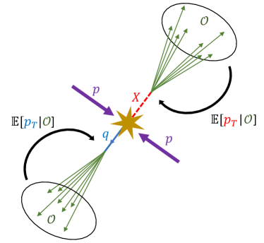
In this paper, we introduce an anomaly detection strategy called FORCE—factorized observables for regressing conditional expectations—based on the inductive bias of factorization. Factorization occurs when the physics governing high-energy scales is approximately independent from those governing low-energy scales. Jet production offers a canonical example of factorization at colliders, where the processes that determine the kinematics and flavors of high-energy partons are approximately independent of the dynamics that yield collimated sprays of low-energy hadrons. As illustrated in Fig. 1, a machine learning model can be trained to predict the kinematics of a jet from its boost-invariant substructure. Kinematics and substructure are approximately independent in the absence of new physics, so if the model learns non-trivial correlations, then this indicates a possible anomaly. Our approach does not require simulated data, works even if the new physics is non-resonant, and provably converges to the optimal classifier in a controlled limit. FORCE builds upon previous uses of factorized structures to estimate backgrounds Cohen et al. (2014); Lin et al. (2019), train data-driven collider classifiers Dery et al. (2017); Cohen et al. (2018); Metodiev et al. (2017); Komiske et al. (2018a); Sirunyan et al. (2020); Amram and Suarez (2021), and disentangle particle flavors using topic modeling Metodiev and Thaler (2018); Komiske et al. (2018b); Aad et al. (2019); Komiske et al. (2022).
To demonstrate the FORCE approach, we perform a case study involving jets Salam (2010); Larkoski et al. (2020); Kogler et al. (2019); Marzani et al. (2019). Jets are proxies for the partons or resonances produced in high-energy collisions, with the kinematics of a jet reflecting the kinematics of its initiating particle. Jets then acquire substructure through lower-energy processes, such as decays of intermediate-scale resonances or showering/hadronization in quantum chromodynamics (QCD). Many new physics scenarios involve jet production, making jets a key target for anomaly detection.
In the soft-collinear limit of QCD, the substructure of a jet factorizes from its kinematics Bauer et al. (2001); Bauer and Stewart (2001); Bauer et al. (2002a, b, b); Beneke et al. (2002) (see also Collins et al. (1989); Bauer et al. (2009); Feige and Schwartz (2014); Sterman (2022)). Factorization also holds for the decay of an intermediate-scale resonance in the narrow width approximation Berdine et al. (2007); Uhlemann and Kauer (2009), such as for a Lorentz-boosted / boson, Higgs boson, or top quark. At leading order, the kinematics of a jet is determined by its transverse momentum and rapidity . Let be a list of jet substructure observables, possibly high dimensional. Then, assuming factorization holds, the distribution of jet kinematics and substructure obey:
| (1) |
where labels the types of initiating particle, and is the fraction of jets initiated by that particle type. Factorization imposes a non-trivial constraint that is independent of and that a finite sum over is sufficient to model the distribution.
If we make an even more restrictive assumption that consists of scale- and boost-invariant observables, with no conditional dependence, then we can write:
| (2) |
Examples of such quasi-invariant observables are -subjettiness ratios Thaler and Van Tilburg (2011, 2012), Larkoski et al. (2014a), Larkoski et al. (2015), and Moult et al. (2016). Here, we take the jet substructure to be dominated by the initiating particle’s flavor and independent of the remainder of the event, up to subleading corrections. The factorized structure of Eqs. (1) and (2) is what we will exploit for anomaly detection using FORCE.
Consider the case of only two jet types: background () QCD jets from high-energy quarks and gluons, and signal () jets from the hadronic decay of a new particle. To simplify the algebra, we marginalize over . Via Eqs. (1) and (2), i.e. assuming and are independent in both the signal and background processes, the joint distribution of jet kinematics and substructure is:
| (3) |
where is the fraction of new physics events and is the fraction of QCD events, with . Our goal is to discover and characterize the new physics signal in a data-driven manner.
The key insight behind FORCE is that a machine-learned model trained to predict from yields the optimal versus classifier in appropriate limits. To see this, recall from the Neyman-Pearson lemma Neyman and Pearson (1992) that the signal-to-background likelihood ratio is the optimal new physics classifier derivable from :
| (4) |
(A stronger classifier might exist if one includes information, but that requires a priori knowledge of .) Further, as reviewed in the Supplemental Material, minimizing the mean-squared error converges—with sufficient statistics, a flexible enough model, and adequate training time—to the conditional expectation value . From Eq. (3), the conditional distribution can be written as
| (5) |
Taking the expectation value with respect to yields:
| (6) |
Remarkably, is monotonically related to , so it also defines optimal decision boundaries. A similar observation underpins anomaly detection methods based on classification without labels Metodiev et al. (2017); Collins et al. (2018, 2019). To our knowledge, the first proof that optimal classifiers can be defined through regression (as opposed to classification) appears in Ref. Komiske et al. (2022).
Thus, assuming Factorized Observables, Regressing the Conditional Expectation furnishes a powerful probe of new physics, justifying the FORCE acronym. Interestingly, the same logic holds with more than one type of new particle, such as , as long as as expected from momentum conservation. If , then Eq. (6) defines an optimal tagger; otherwise, it defines an optimal anti-tagger. In the absence of new physics () or if the signal and background have the same average kinematics (), then Eq. (6) simply returns the expectation value with no observable dependence. Deviations of the model output from are therefore a harbinger for a new type of factorized object in the data (or a violation of the factorization assumption).
In summary, FORCE proceeds as follows:
-
1.
Define approximately factorized objects (e.g. jets) with kinematics and scale-/boost-invariant substructure .
-
2.
Train a machine-learning model to predict from with the mean-squared error loss.
-
3.
Classify anomalous objects via the model output.
Of course, real collider data is richer than the simple two-category case in Eq. (3). QCD jets themselves are admixtures of quark and gluon jets, each with slightly different kinematics and substructure. Multiple effects can violate factorization, such as partial containment of particle decay products in the jet cone or the logarithmic scale-dependence of QCD due to the running of the strong coupling constant. Further, certain known Standard-Model processes, such as jets from hadronically decaying //Higgs bosons or top quarks, may be considered anomalous beyond the QCD dijet background by our formulation. This behavior may in fact be desirable, and “re-discovering” these particles may be an interesting way to benchmark this technique in data. More broadly, though, the general structure of factorization motivates FORCE as a new physics search strategy.
We now showcase FORCE for a new physics search involving dijets. Our case study is based on the development dataset Kasieczka et al. (2019) from the LHC Olympics 2020 Anomaly Detection Challenge Kasieczka et al. (2021a). This simulated dataset consists of 1 million QCD dijet events and up to 100 thousand events, with the and particles decaying to two quarks. The masses of the three new particles are TeV, GeV, and GeV. The and particles are boosted, giving rise to a dijet resonance with two-pronged jet substructure. While the signal has a mass peak, this feature is not used for FORCE training.
The LHC Olympics dataset is generated with Pythia 8.219 Sjostrand et al. (2008); Sjöstrand et al. (2015) and simulated with Delphes 3.4.1 de Favereau et al. (2014), excluding pileup or multiple parton interactions. Events are selected to have at least one anti- Cacciari et al. (2008) jet with transverse momentum TeV and pseudorapidity . Jets are clustered via the anti- algorithm with a radius of using FastJet 3.3.3 Cacciari et al. (2008, 2012). The leading two jets, i.e. those with highest transverse momenta, are recorded in each event as a proxy for the products of the high-energy scattering process. Both jets are used in the analysis, so the anomalies are defined over jets (instead of over events).
For our substructure observables , we use energy flow polynomials (EFPs) Komiske et al. (2018c, 2020a). As reviewed in the Supplemental Material, EFPs arise from a systematic expansion in energies and angles, and they are sensitive to a broad range of jet features. We compute all 13 EFPs up to and including degree 3 using EnergyFlow 1.0.3 Komiske and Metodiev (2019), using as the energy variable and as the angular variable. To satisfy Eq. (2), the EFPs need to be made scale- and boost-invariant. Quasi-scale-invariance can be achieved by normalizing the energies to sum to unity. As transverse boosts approximately scale energies by and angles by , the EFPs can be made quasi-boost-invariant by rescaling them via:
| (7) |
where and are the energy and angular degrees of the polynomial. This rescaling reduces our basis to seven independent elements. We note that observables desired to be independent of have been employed in prior work on anomaly detection Collins et al. (2019) and jet-tagging Aguilar-Saavedra et al. (2017). In the Supplemental Material, we show how FORCE performance degrades without this normalization. Interestingly, existing observables for multi-prong new physics searches, such as Larkoski et al. (2014a), emerge naturally as elements of this quasi-invariant basis.
The FORCE method works with any machine-learning algorithm that converges to the conditional expectation . We use a fully-connected neural network consisting of three dense layers with 50 nodes per layer, as well as L2 kernel and bias regularization of in each layer. Between each dense layer is a dropout Srivastava et al. (2014) layer with . Neural networks are implemented and trained with Keras Chollet (2017) using TensorFlow Abadi et al. (2016), optimized with ADAM Kingma and Ba (2017) with a patience parameter of 10. Since our method is fully unsupervised, seeing no signal/background labels, we utilize the full dataset in training. Our code implementing FORCE is publicly available on GitHub Wynne (2023).
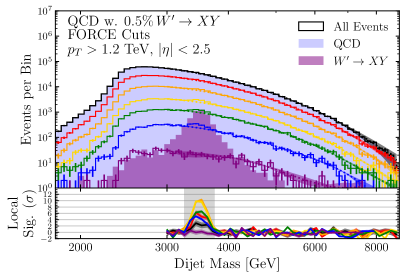
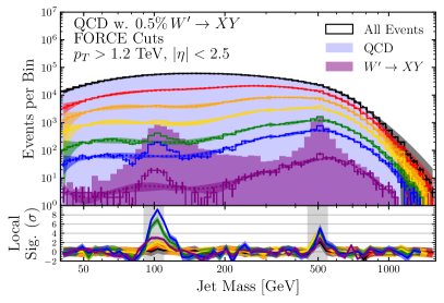
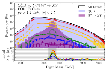
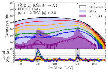
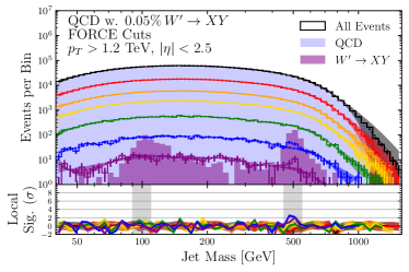
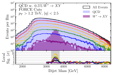
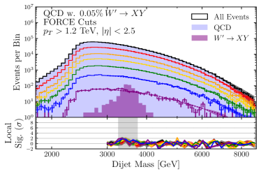
The dijet and jet mass distributions are shown in Fig. 2 after applying FORCE for a signal fraction of . Here, both jets have to pass the same cut on the model output. With a strict enough cut, the signal clearly manifests as a peak at TeV in the dijet mass distribution, and peaks at GeV and GeV in the individual jet mass distribution. To estimate the local significance, a background fit is performed using Legendre polynomials outside of the shaded signal region, using fifth order as the central value and between second and seventh orders for the uncertainty band. For the dijet mass background fit, we use data above TeV, and for the jet mass background fits, below GeV for and above GeV for . We find a boost in significance, where a pre-cut excess of for the and are increased to , while a pre-cut excess of for the is increased to . Note that although the new physics in this case study appears as a resonance in the jet and dijet mass distributions, a resonance is not a requirement of the FORCE method. (Without a bump-like feature, though, one would have to leverage some other method for background estimation.) Further, by imposing quasi-boost/scale invariance, the model output is largely decorrelated from jet mass (see related discussion in Refs. Dolen et al. (2016); Shimmin et al. (2017); Moult et al. (2018)).
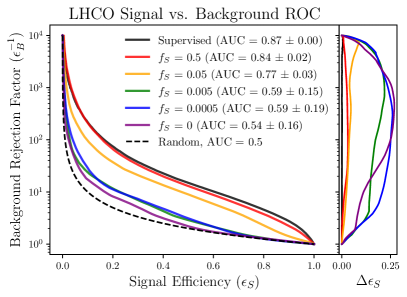
To test the robustness of FORCE, we apply the our method on range of signal fractions . For stability in this analysis, we train with an equally mixed dataset of 100,000 signal and 100,000 background events, using sample weights in Keras to mimic a signal fraction . We then test the model on the full dataset. The per-jet classification performance is shown in Fig. 3, where we plot the background rejection factor as a function of signal efficiency. We also show the standard deviation in signal efficiency after performing 10 trainings. Here, the per-jet performance is evaluated only on the learned , not including any additional features such as jet mass or assumptions about the event topology. (For these reasons, one cannot directly compare our results to those of previous LHC Olympians.) In the large signal limit, FORCE approaches the optimal supervised classifier, as predicted by Eq. (6). As the signal fraction decreases, the performance degrades and the variability increases, but there are still substantial gains in sensitivity. Note that the limit still yields reasonable classification performance; this is possibly due to deviations from strict factorization, as discussed further in the Supplemental Material. (Alternatively, since we are applying a no-signal model to a dataset with signal, proper convergence might not be achievable off the data manifold.)
Having established the desired behavior of FORCE on a benchmark collider search, it is worth remarking on several important points. First, our method is based on the inductive bias of factorization, so the performance we saw in the dijet analysis may not translate to other scenarios. This reflects a universal challenge for all approaches to anomaly detection, where the performance of the method depends on the applicability of the assumptions. Nevertheless, limits can be set on the parameters of specific new physics scenarios (even post hoc) by performing pseudo-experiments, injecting various amounts of signal, and repeating the procedure to establish confidence intervals. Second, as the signal fraction decreases, the performance of the learned model becomes highly sensitive to parameter initialization and statistical fluctuations. To ensure robust behavior in this regime, we recommend FORCE be paired with a regularization method like ensemble learning Ganaie et al. (2021). Third, detector effects can introduce factorization-violating effects, so it may be beneficial to apply FORCE after multi-dimensional unfolding is applied to the data Andreassen et al. (2020b); Bellagente et al. (2020); Andreassen et al. (2021); Arratia et al. (2022). Jet grooming techniques Dasgupta et al. (2013); Larkoski et al. (2014b); Frye et al. (2016) might also improve the factorized behavior of jets at the theoretical level. Finally, we emphasize that no strategy can outperform a targeted search (i.e. hypothesis test) for a specific model, and that the power of data-driven approaches such as FORCE is in broadening the space of new physics scenarios that can be probed.
In summary, we introduced FORCE: an anomaly detection strategy for factorized new physics. By training a machine-learning model to predict the kinematics of factorized objects from their scale- and boost-invariant substructure, we obtain a powerful classifier directly from observed data. We showcased FORCE on a benchmark search for new physics in the dijet final state, where it successfully identified a new physics signal. This work contributes to a growing body of work where powerful computational tools from machine learning are combined with deep theoretical principles to unlock novel collider data analysis strategies. Furthermore, the FORCE method can be easily integrated into these prior methods when viewing the model output as an observable with high discrimination power.
The FORCE framework shifts the discussion of new physics searches from specific models to their general factorized structure, with machine-learning techniques performing detailed observable-level analyses. It would be interesting to generalize FORCE to handle more than one kinematic feature and more than two event categories, which would be important to handle multiple background components. It would also be interesting to combine our reasoning with the factorization of the full event energy flow Bauer et al. (2009), which may help reframe anomaly detection in the language of “theory space” Komiske et al. (2019, 2020b). Though we focused on jets and jet substructure here, this method applies more broadly to any factorized probability distributions, in collider physics and beyond. Data-driven searches hold the potential to fundamentally surprise us, not only by discovering new physics, but by uncovering it in forms that we have failed to imagine.
Acknowledgements.
The authors are grateful to the organizers of the LHC Olympics 2020 Anomaly Detection Challenge for stimulating this research direction and producing excellent public datasets. We are grateful to Samuel Alipour-fard, Rikab Gambhir, Patrick Komiske, Benjamin Nachman, and Nilai Sarda for helpful comments and discussions. JT is supported by the National Science Foundation under Cooperative Agreement PHY-2019786 (The NSF AI Institute for Artificial Intelligence and Fundamental Interactions) and by the Simons Foundation through Investigator grant 929241. This work was supported by the Office of Nuclear Physics of the U.S. Department of Energy (DOE) under Grant No. DE-SC0011090 and by the DOE Office of High Energy Physics under grants DE-SC0012567 and DE-SC0019128.References
- Aad et al. (2012) Georges Aad et al. (ATLAS), “Observation of a new particle in the search for the Standard Model Higgs boson with the ATLAS detector at the LHC,” Phys. Lett. B 716, 1–29 (2012), arXiv:1207.7214 [hep-ex] .
- Chatrchyan et al. (2012) Serguei Chatrchyan et al. (CMS), “Observation of a New Boson at a Mass of 125 GeV with the CMS Experiment at the LHC,” Phys. Lett. B 716, 30–61 (2012), arXiv:1207.7235 [hep-ex] .
- Aguilar-Saavedra et al. (2017) J. A. Aguilar-Saavedra, Jack H. Collins, and Rashmish K. Mishra, “A generic anti-QCD jet tagger,” JHEP 11, 163 (2017), arXiv:1709.01087 [hep-ph] .
- Collins et al. (2018) Jack H. Collins, Kiel Howe, and Benjamin Nachman, “Anomaly Detection for Resonant New Physics with Machine Learning,” Phys. Rev. Lett. 121, 241803 (2018), arXiv:1805.02664 [hep-ph] .
- D’Agnolo and Wulzer (2019) Raffaele Tito D’Agnolo and Andrea Wulzer, “Learning New Physics from a Machine,” Phys. Rev. D 99, 015014 (2019), arXiv:1806.02350 [hep-ph] .
- De Simone and Jacques (2019) Andrea De Simone and Thomas Jacques, “Guiding New Physics Searches with Unsupervised Learning,” Eur. Phys. J. C 79, 289 (2019), arXiv:1807.06038 [hep-ph] .
- Hajer et al. (2020) Jan Hajer, Ying-Ying Li, Tao Liu, and He Wang, “Novelty Detection Meets Collider Physics,” Phys. Rev. D 101, 076015 (2020), arXiv:1807.10261 [hep-ph] .
- Farina et al. (2020) Marco Farina, Yuichiro Nakai, and David Shih, “Searching for New Physics with Deep Autoencoders,” Phys. Rev. D 101, 075021 (2020), arXiv:1808.08992 [hep-ph] .
- Heimel et al. (2019) Theo Heimel, Gregor Kasieczka, Tilman Plehn, and Jennifer M. Thompson, “QCD or What?” SciPost Phys. 6, 030 (2019), arXiv:1808.08979 [hep-ph] .
- Casa and Menardi (2018) Alessandro Casa and Giovanna Menardi, “Nonparametric semisupervised classification for signal detection in high energy physics,” (2018), arXiv:1809.02977 [stat.AP] .
- Cerri et al. (2019) Olmo Cerri, Thong Q. Nguyen, Maurizio Pierini, Maria Spiropulu, and Jean-Roch Vlimant, “Variational Autoencoders for New Physics Mining at the Large Hadron Collider,” JHEP 05, 036 (2019), arXiv:1811.10276 [hep-ex] .
- Collins et al. (2019) Jack H. Collins, Kiel Howe, and Benjamin Nachman, “Extending the search for new resonances with machine learning,” Phys. Rev. D 99, 014038 (2019), arXiv:1902.02634 [hep-ph] .
- Roy and Vijay (2019) Tuhin S. Roy and Aravind H. Vijay, “A robust anomaly finder based on autoencoders,” (2019), arXiv:1903.02032 [hep-ph] .
- Dillon et al. (2019) Barry M. Dillon, Darius A. Faroughy, and Jernej F. Kamenik, “Uncovering latent jet substructure,” Phys. Rev. D 100, 056002 (2019), arXiv:1904.04200 [hep-ph] .
- Blance et al. (2019) Andrew Blance, Michael Spannowsky, and Philip Waite, “Adversarially-trained autoencoders for robust unsupervised new physics searches,” JHEP 10, 047 (2019), arXiv:1905.10384 [hep-ph] .
- Romão Crispim et al. (2020) M. Romão Crispim, N. F. Castro, R. Pedro, and T. Vale, “Transferability of Deep Learning Models in Searches for New Physics at Colliders,” Phys. Rev. D 101, 035042 (2020), arXiv:1912.04220 [hep-ph] .
- Mullin et al. (2021) Anna Mullin, Stuart Nicholls, Holly Pacey, Michael Parker, Martin White, and Sarah Williams, “Does SUSY have friends? A new approach for LHC event analysis,” JHEP 02, 160 (2021), arXiv:1912.10625 [hep-ph] .
- D’Agnolo et al. (2021) Raffaele Tito D’Agnolo, Gaia Grosso, Maurizio Pierini, Andrea Wulzer, and Marco Zanetti, “Learning multivariate new physics,” Eur. Phys. J. C 81, 89 (2021), arXiv:1912.12155 [hep-ph] .
- Nachman and Shih (2020) Benjamin Nachman and David Shih, “Anomaly Detection with Density Estimation,” Phys. Rev. D 101, 075042 (2020), arXiv:2001.04990 [hep-ph] .
- Andreassen et al. (2020a) Anders Andreassen, Benjamin Nachman, and David Shih, “Simulation Assisted Likelihood-free Anomaly Detection,” Phys. Rev. D 101, 095004 (2020a), arXiv:2001.05001 [hep-ph] .
- Amram and Suarez (2021) Oz Amram and Cristina Mantilla Suarez, “Tag N’ Train: a technique to train improved classifiers on unlabeled data,” JHEP 01, 153 (2021), arXiv:2002.12376 [hep-ph] .
- Crispim Romão et al. (2021a) M. Crispim Romão, N. F. Castro, J. G. Milhano, R. Pedro, and T. Vale, “Use of a generalized energy Mover’s distance in the search for rare phenomena at colliders,” Eur. Phys. J. C 81, 192 (2021a), arXiv:2004.09360 [hep-ph] .
- Knapp et al. (2021) Oliver Knapp, Olmo Cerri, Guenther Dissertori, Thong Q. Nguyen, Maurizio Pierini, and Jean-Roch Vlimant, “Adversarially Learned Anomaly Detection on CMS Open Data: re-discovering the top quark,” Eur. Phys. J. Plus 136, 236 (2021), arXiv:2005.01598 [hep-ex] .
- Aad et al. (2020) Georges Aad et al. (ATLAS), “Dijet resonance search with weak supervision using TeV collisions in the ATLAS detector,” Phys. Rev. Lett. 125, 131801 (2020), arXiv:2005.02983 [hep-ex] .
- Dillon et al. (2020) B. M. Dillon, D. A. Faroughy, J. F. Kamenik, and M. Szewc, “Learning the latent structure of collider events,” JHEP 10, 206 (2020), arXiv:2005.12319 [hep-ph] .
- Crispim Romão et al. (2021b) M. Crispim Romão, N. F. Castro, and R. Pedro, “Finding New Physics without learning about it: Anomaly Detection as a tool for Searches at Colliders,” Eur. Phys. J. C 81, 27 (2021b), [Erratum: Eur.Phys.J.C 81, 1020 (2021)], arXiv:2006.05432 [hep-ph] .
- Cheng et al. (2023) Taoli Cheng, Jean-François Arguin, Julien Leissner-Martin, Jacinthe Pilette, and Tobias Golling, “Variational autoencoders for anomalous jet tagging,” Phys. Rev. D 107, 016002 (2023), arXiv:2007.01850 [hep-ph] .
- Khosa and Sanz (2023) Charanjit Kaur Khosa and Veronica Sanz, “Anomaly Awareness,” SciPost Phys. 15, 053 (2023), arXiv:2007.14462 [cs.LG] .
- Thaprasop et al. (2021) Punnathat Thaprasop, Kai Zhou, Jan Steinheimer, and Christoph Herold, “Unsupervised Outlier Detection in Heavy-Ion Collisions,” Phys. Scripta 96, 064003 (2021), arXiv:2007.15830 [hep-ex] .
- Aguilar-Saavedra et al. (2021) J. A. Aguilar-Saavedra, F. R. Joaquim, and J. F. Seabra, “Mass Unspecific Supervised Tagging (MUST) for boosted jets,” JHEP 03, 012 (2021), [Erratum: JHEP 04, 133 (2021)], arXiv:2008.12792 [hep-ph] .
- Alexander et al. (2020) Stephon Alexander, Sergei Gleyzer, Hanna Parul, Pranath Reddy, Michael W. Toomey, Emanuele Usai, and Ryker Von Klar, “Decoding Dark Matter Substructure without Supervision,” (2020), arXiv:2008.12731 [astro-ph.CO] .
- Benkendorfer et al. (2021) Kees Benkendorfer, Luc Le Pottier, and Benjamin Nachman, “Simulation-assisted decorrelation for resonant anomaly detection,” Phys. Rev. D 104, 035003 (2021), arXiv:2009.02205 [hep-ph] .
- Pol et al. (2020) Adrian Alan Pol, Victor Berger, Gianluca Cerminara, Cecile Germain, and Maurizio Pierini, “Anomaly Detection With Conditional Variational Autoencoders,” in Eighteenth International Conference on Machine Learning and Applications (2020) arXiv:2010.05531 [cs.LG] .
- Mikuni and Canelli (2021) Vinicius Mikuni and Florencia Canelli, “Unsupervised clustering for collider physics,” Phys. Rev. D 103, 092007 (2021), arXiv:2010.07106 [physics.data-an] .
- van Beekveld et al. (2021) Melissa van Beekveld, Sascha Caron, Luc Hendriks, Paul Jackson, Adam Leinweber, Sydney Otten, Riley Patrick, Roberto Ruiz De Austri, Marco Santoni, and Martin White, “Combining outlier analysis algorithms to identify new physics at the LHC,” JHEP 09, 024 (2021), arXiv:2010.07940 [hep-ph] .
- Park et al. (2020) Sang Eon Park, Dylan Rankin, Silviu-Marian Udrescu, Mikaeel Yunus, and Philip Harris, “Quasi Anomalous Knowledge: Searching for new physics with embedded knowledge,” JHEP 21, 030 (2020), arXiv:2011.03550 [hep-ph] .
- Faroughy (2021) Darius A. Faroughy, “Uncovering hidden new physics patterns in collider events using Bayesian probabilistic models,” PoS ICHEP2020, 238 (2021), arXiv:2012.08579 [hep-ph] .
- Stein et al. (2020) George Stein, Uros Seljak, and Biwei Dai, “Unsupervised in-distribution anomaly detection of new physics through conditional density estimation,” in 34th Conference on Neural Information Processing Systems (2020) arXiv:2012.11638 [cs.LG] .
- Kasieczka et al. (2021a) Gregor Kasieczka et al., “The LHC Olympics 2020 a community challenge for anomaly detection in high energy physics,” Rept. Prog. Phys. 84, 124201 (2021a), arXiv:2101.08320 [hep-ph] .
- Chakravarti et al. (2021) Purvasha Chakravarti, Mikael Kuusela, Jing Lei, and Larry Wasserman, “Model-Independent Detection of New Physics Signals Using Interpretable Semi-Supervised Classifier Tests,” (2021), arXiv:2102.07679 [stat.AP] .
- Batson et al. (2021) Joshua Batson, C. Grace Haaf, Yonatan Kahn, and Daniel A. Roberts, “Topological Obstructions to Autoencoding,” JHEP 04, 280 (2021), arXiv:2102.08380 [hep-ph] .
- Blance and Spannowsky (2020) Andrew Blance and Michael Spannowsky, “Unsupervised event classification with graphs on classical and photonic quantum computers,” JHEP 21, 170 (2020), arXiv:2103.03897 [hep-ph] .
- Bortolato et al. (2022) Blaž Bortolato, Aleks Smolkovič, Barry M. Dillon, and Jernej F. Kamenik, “Bump hunting in latent space,” Phys. Rev. D 105, 115009 (2022), arXiv:2103.06595 [hep-ph] .
- Collins et al. (2021) Jack H. Collins, Pablo Martín-Ramiro, Benjamin Nachman, and David Shih, “Comparing weak- and unsupervised methods for resonant anomaly detection,” Eur. Phys. J. C 81, 617 (2021), arXiv:2104.02092 [hep-ph] .
- Dillon et al. (2021) Barry M. Dillon, Tilman Plehn, Christof Sauer, and Peter Sorrenson, “Better Latent Spaces for Better Autoencoders,” SciPost Phys. 11, 061 (2021), arXiv:2104.08291 [hep-ph] .
- Finke et al. (2021) Thorben Finke, Michael Krämer, Alessandro Morandini, Alexander Mück, and Ivan Oleksiyuk, “Autoencoders for unsupervised anomaly detection in high energy physics,” JHEP 06, 161 (2021), arXiv:2104.09051 [hep-ph] .
- Shih et al. (2021) David Shih, Matthew R. Buckley, Lina Necib, and John Tamanas, “via machinae: Searching for stellar streams using unsupervised machine learning,” Mon. Not. Roy. Astron. Soc. 509, 5992–6007 (2021), arXiv:2104.12789 [astro-ph.GA] .
- Atkinson et al. (2021) Oliver Atkinson, Akanksha Bhardwaj, Christoph Englert, Vishal S. Ngairangbam, and Michael Spannowsky, “Anomaly detection with convolutional Graph Neural Networks,” JHEP 08, 080 (2021), arXiv:2105.07988 [hep-ph] .
- Kahn et al. (2021) Alan Kahn, Julia Gonski, Inês Ochoa, Daniel Williams, and Gustaaf Brooijmans, “Anomalous jet identification via sequence modeling,” JINST 16, P08012 (2021), arXiv:2105.09274 [hep-ph] .
- Aarrestad et al. (2022) Thea Aarrestad et al., “The Dark Machines Anomaly Score Challenge: Benchmark Data and Model Independent Event Classification for the Large Hadron Collider,” SciPost Phys. 12, 043 (2022), arXiv:2105.14027 [hep-ph] .
- Dorigo et al. (2023) Tommaso Dorigo, Martina Fumanelli, Chiara Maccani, Marija Mojsovska, Giles C. Strong, and Bruno Scarpa, “RanBox: anomaly detection in the copula space,” JHEP 01, 008 (2023), arXiv:2106.05747 [physics.data-an] .
- Caron et al. (2022) Sascha Caron, Luc Hendriks, and Rob Verheyen, “Rare and Different: Anomaly Scores from a combination of likelihood and out-of-distribution models to detect new physics at the LHC,” SciPost Phys. 12, 077 (2022), arXiv:2106.10164 [hep-ph] .
- Govorkova et al. (2022a) Ekaterina Govorkova, Ema Puljak, Thea Aarrestad, Maurizio Pierini, Kinga Anna Woźniak, and Jennifer Ngadiuba, “LHC physics dataset for unsupervised New Physics detection at 40 MHz,” Sci. Data 9, 118 (2022a), arXiv:2107.02157 [physics.data-an] .
- Kasieczka et al. (2021b) Gregor Kasieczka, Benjamin Nachman, and David Shih, “New Methods and Datasets for Group Anomaly Detection From Fundamental Physics,” in Conference on Knowledge Discovery and Data Mining (2021) arXiv:2107.02821 [stat.ML] .
- Volkovich et al. (2022) Sergey Volkovich, Federico De Vito Halevy, and Shikma Bressler, “A data-directed paradigm for BSM searches: the bump-hunting example,” Eur. Phys. J. C 82, 265 (2022), arXiv:2107.11573 [hep-ex] .
- Govorkova et al. (2022b) Ekaterina Govorkova et al., “Autoencoders on field-programmable gate arrays for real-time, unsupervised new physics detection at 40 MHz at the Large Hadron Collider,” Nature Mach. Intell. 4, 154–161 (2022b), arXiv:2108.03986 [physics.ins-det] .
- Hallin et al. (2022) Anna Hallin, Joshua Isaacson, Gregor Kasieczka, Claudius Krause, Benjamin Nachman, Tobias Quadfasel, Matthias Schlaffer, David Shih, and Manuel Sommerhalder, “Classifying anomalies through outer density estimation,” Phys. Rev. D 106, 055006 (2022), arXiv:2109.00546 [hep-ph] .
- Ostdiek (2022) Bryan Ostdiek, “Deep Set Auto Encoders for Anomaly Detection in Particle Physics,” SciPost Phys. 12, 045 (2022), arXiv:2109.01695 [hep-ph] .
- Fraser et al. (2022) Katherine Fraser, Samuel Homiller, Rashmish K. Mishra, Bryan Ostdiek, and Matthew D. Schwartz, “Challenges for unsupervised anomaly detection in particle physics,” JHEP 03, 066 (2022), arXiv:2110.06948 [hep-ph] .
- Jawahar et al. (2022) Pratik Jawahar, Thea Aarrestad, Nadezda Chernyavskaya, Maurizio Pierini, Kinga A. Wozniak, Jennifer Ngadiuba, Javier Duarte, and Steven Tsan, “Improving Variational Autoencoders for New Physics Detection at the LHC With Normalizing Flows,” Front. Big Data 5, 803685 (2022), arXiv:2110.08508 [hep-ph] .
- Herrero-Garcia et al. (2022) Juan Herrero-Garcia, Riley Patrick, and Andre Scaffidi, “A semi-supervised approach to dark matter searches in direct detection data with machine learning,” JCAP 02, 039 (2022), arXiv:2110.12248 [hep-ph] .
- Lester and Tombs (2021) Christopher G. Lester and Rupert Tombs, “Using unsupervised learning to detect broken symmetries, with relevance to searches for parity violation in nature. (Previously: ”Stressed GANs snag desserts”),” (2021), arXiv:2111.00616 [hep-ph] .
- Aguilar-Saavedra (2022a) J. A. Aguilar-Saavedra, “Anomaly detection from mass unspecific jet tagging,” Eur. Phys. J. C 82, 130 (2022a), arXiv:2111.02647 [hep-ph] .
- Tombs and Lester (2022) Rupert Tombs and Christopher G. Lester, “A method to challenge symmetries in data with self-supervised learning,” JINST 17, P08024 (2022), arXiv:2111.05442 [hep-ph] .
- Mikuni et al. (2022) Vinicius Mikuni, Benjamin Nachman, and David Shih, “Online-compatible unsupervised nonresonant anomaly detection,” Phys. Rev. D 105, 055006 (2022), arXiv:2111.06417 [cs.LG] .
- Chekanov and Hopkins (2022) Sergei Chekanov and Walter Hopkins, “Event-Based Anomaly Detection for Searches for New Physics,” Universe 8, 494 (2022), arXiv:2111.12119 [hep-ph] .
- d’Agnolo et al. (2022) Raffaele Tito d’Agnolo, Gaia Grosso, Maurizio Pierini, Andrea Wulzer, and Marco Zanetti, “Learning new physics from an imperfect machine,” Eur. Phys. J. C 82, 275 (2022), arXiv:2111.13633 [hep-ph] .
- Canelli et al. (2022) Florencia Canelli, Annapaola de Cosa, Luc Le Pottier, Jeremi Niedziela, Kevin Pedro, and Maurizio Pierini, “Autoencoders for semivisible jet detection,” JHEP 02, 074 (2022), arXiv:2112.02864 [hep-ph] .
- Ngairangbam et al. (2022) Vishal S. Ngairangbam, Michael Spannowsky, and Michihisa Takeuchi, “Anomaly detection in high-energy physics using a quantum autoencoder,” Phys. Rev. D 105, 095004 (2022), arXiv:2112.04958 [hep-ph] .
- Aguilar-Saavedra (2022b) J. A. Aguilar-Saavedra, “Taming modeling uncertainties with mass unspecific supervised tagging,” Eur. Phys. J. C 82, 270 (2022b), arXiv:2201.11143 [hep-ph] .
- Buss et al. (2023) Thorsten Buss, Barry M. Dillon, Thorben Finke, Michael Krämer, Alessandro Morandini, Alexander Mück, Ivan Oleksiyuk, and Tilman Plehn, “What’s anomalous in LHC jets?” SciPost Phys. 15, 168 (2023), arXiv:2202.00686 [hep-ph] .
- Bradshaw et al. (2022) Layne Bradshaw, Spencer Chang, and Bryan Ostdiek, “Creating simple, interpretable anomaly detectors for new physics in jet substructure,” Phys. Rev. D 106, 035014 (2022), arXiv:2203.01343 [hep-ph] .
- Birman et al. (2022) Mattias Birman, Benjamin Nachman, Raphael Sebbah, Gal Sela, Ophir Turetz, and Shikma Bressler, “Data-directed search for new physics based on symmetries of the SM,” Eur. Phys. J. C 82, 508 (2022), arXiv:2203.07529 [hep-ph] .
- Raine et al. (2023) John Andrew Raine, Samuel Klein, Debajyoti Sengupta, and Tobias Golling, “CURTAINs for your sliding window: Constructing unobserved regions by transforming adjacent intervals,” Front. Big Data 6, 899345 (2023), arXiv:2203.09470 [hep-ph] .
- Letizia et al. (2022) Marco Letizia, Gianvito Losapio, Marco Rando, Gaia Grosso, Andrea Wulzer, Maurizio Pierini, Marco Zanetti, and Lorenzo Rosasco, “Learning new physics efficiently with nonparametric methods,” Eur. Phys. J. C 82, 879 (2022), arXiv:2204.02317 [hep-ph] .
- Fanelli et al. (2022) C. Fanelli, J. Giroux, and Z. Papandreou, “‘Flux+Mutability’: a conditional generative approach to one-class classification and anomaly detection,” Mach. Learn. Sci. Tech. 3, 045012 (2022), arXiv:2204.08609 [cs.LG] .
- Finke et al. (2022) Thorben Finke, Michael Krämer, Maximilian Lipp, and Alexander Mück, “Boosting mono-jet searches with model-agnostic machine learning,” JHEP 08, 015 (2022), arXiv:2204.11889 [hep-ph] .
- Verheyen (2022) Rob Verheyen, “Event Generation and Density Estimation with Surjective Normalizing Flows,” SciPost Phys. 13, 047 (2022), arXiv:2205.01697 [hep-ph] .
- Dillon et al. (2022a) Barry M. Dillon, Radha Mastandrea, and Benjamin Nachman, “Self-supervised anomaly detection for new physics,” Phys. Rev. D 106, 056005 (2022a), arXiv:2205.10380 [hep-ph] .
- Alvi et al. (2023) Sulaiman Alvi, Christian W. Bauer, and Benjamin Nachman, “Quantum anomaly detection for collider physics,” JHEP 02, 220 (2023), arXiv:2206.08391 [hep-ph] .
- Dillon et al. (2022b) Barry M. Dillon, Luigi Favaro, Tilman Plehn, Peter Sorrenson, and Michael Krämer, “A Normalized Autoencoder for LHC Triggers,” (2022b), arXiv:2206.14225 [hep-ph] .
- Caron et al. (2023) Sascha Caron, Roberto Ruiz de Austri, and Zhongyi Zhang, “Mixture-of-Theories training: can we find new physics and anomalies better by mixing physical theories?” JHEP 03, 004 (2023), arXiv:2207.07631 [hep-ph] .
- Park et al. (2023) Sang Eon Park, Philip Harris, and Bryan Ostdiek, “Neural embedding: learning the embedding of the manifold of physics data,” JHEP 07, 108 (2023), arXiv:2208.05484 [hep-ph] .
- Kasieczka et al. (2023) Gregor Kasieczka, Radha Mastandrea, Vinicius Mikuni, Benjamin Nachman, Mariel Pettee, and David Shih, “Anomaly detection under coordinate transformations,” Phys. Rev. D 107, 015009 (2023), arXiv:2209.06225 [hep-ph] .
- Kamenik and Szewc (2023) Jernej F. Kamenik and Manuel Szewc, “Null hypothesis test for anomaly detection,” Phys. Lett. B 840, 137836 (2023), arXiv:2210.02226 [hep-ph] .
- Hallin et al. (2023) Anna Hallin, Gregor Kasieczka, Tobias Quadfasel, David Shih, and Manuel Sommerhalder, “Resonant anomaly detection without background sculpting,” Phys. Rev. D 107, 114012 (2023), arXiv:2210.14924 [hep-ph] .
- Araz and Spannowsky (2022) Jack Y. Araz and Michael Spannowsky, “Quantum-probabilistic Hamiltonian learning for generative modelling & anomaly detection,” (2022), arXiv:2211.03803 [quant-ph] .
- Mastandrea and Nachman (2022) Radha Mastandrea and Benjamin Nachman, “Efficiently Moving Instead of Reweighting Collider Events with Machine Learning,” in 36th Conference on Neural Information Processing Systems: Workshop on Machine Learning and the Physical Sciences (2022) arXiv:2212.06155 [hep-ph] .
- Schuhmacher et al. (2023) Julian Schuhmacher, Laura Boggia, Vasilis Belis, Ema Puljak, Michele Grossi, Maurizio Pierini, Sofia Vallecorsa, Francesco Tacchino, Panagiotis Barkoutsos, and Ivano Tavernelli, “Unravelling physics beyond the standard model with classical and quantum anomaly detection,” Mach. Learn. Sci. Tech. 4, 045031 (2023), arXiv:2301.10787 [hep-ex] .
- Golling et al. (2023a) Tobias Golling et al., “The Mass-ive Issue: Anomaly Detection in Jet Physics,” in 34th Conference on Neural Information Processing Systems (2023) arXiv:2303.14134 [hep-ph] .
- Roche et al. (2023) Stephen Roche, Quincy Bayer, Benjamin Carlson, William Ouligian, Pavel Serhiayenka, Joerg Stelzer, and Tae Min Hong, “Nanosecond anomaly detection with decision trees for high energy physics and real-time application to exotic Higgs decays,” (2023), arXiv:2304.03836 [hep-ex] .
- Sengupta et al. (2023) Debajyoti Sengupta, Samuel Klein, John Andrew Raine, and Tobias Golling, “CURTAINs Flows For Flows: Constructing Unobserved Regions with Maximum Likelihood Estimation,” (2023), arXiv:2305.04646 [hep-ph] .
- Vaslin et al. (2023) Louis Vaslin, Vincent Barra, and Julien Donini, “GAN-AE: an anomaly detection algorithm for New Physics search in LHC data,” Eur. Phys. J. C 83, 1008 (2023), arXiv:2305.15179 [hep-ex] .
- Aad et al. (2023) Georges Aad et al. (ATLAS), “Anomaly detection search for new resonances decaying into a Higgs boson and a generic new particle in hadronic final states using TeV collisions with the ATLAS detector,” (2023), arXiv:2306.03637 [hep-ex] .
- Mikuni and Nachman (2023) Vinicius Mikuni and Benjamin Nachman, “High-dimensional and Permutation Invariant Anomaly Detection,” (2023), arXiv:2306.03933 [hep-ph] .
- Golling et al. (2023b) Tobias Golling, Gregor Kasieczka, Claudius Krause, Radha Mastandrea, Benjamin Nachman, John Andrew Raine, Debajyoti Sengupta, David Shih, and Manuel Sommerhalder, “The Interplay of Machine Learning–based Resonant Anomaly Detection Methods,” (2023b), arXiv:2307.11157 [hep-ph] .
- Chekanov and Zhang (2023) Sergei V. Chekanov and Rui Zhang, “Boosting sensitivity to new physics with unsupervised anomaly detection in dijet resonance search,” (2023), arXiv:2308.02671 [hep-ex] .
- Abadjiev et al. (2023) D. Abadjiev et al. (CMS ECAL), “Autoencoder-based Anomaly Detection System for Online Data Quality Monitoring of the CMS Electromagnetic Calorimeter,” (2023), arXiv:2309.10157 [physics.ins-det] .
- Bickendorf et al. (2023) Gerrit Bickendorf, Manuel Drees, Gregor Kasieczka, Claudius Krause, and David Shih, “Combining Resonant and Tail-based Anomaly Detection,” (2023), arXiv:2309.12918 [hep-ph] .
- Finke et al. (2023) Thorben Finke, Marie Hein, Gregor Kasieczka, Michael Krämer, Alexander Mück, Parada Prangchaikul, Tobias Quadfasel, David Shih, and Manuel Sommerhalder, “Back To The Roots: Tree-Based Algorithms for Weakly Supervised Anomaly Detection,” (2023), arXiv:2309.13111 [hep-ph] .
- Buhmann et al. (2023) Erik Buhmann, Cedric Ewen, Gregor Kasieczka, Vinicius Mikuni, Benjamin Nachman, and David Shih, “Full Phase Space Resonant Anomaly Detection,” (2023), arXiv:2310.06897 [hep-ph] .
- Freytsis et al. (2023) Marat Freytsis, Maxim Perelstein, and Yik Chuen San, “Anomaly Detection in Presence of Irrelevant Features,” (2023), arXiv:2310.13057 [hep-ph] .
- Cohen et al. (2014) Timothy Cohen, Martin Jankowiak, Mariangela Lisanti, Hou Keong Lou, and Jay G. Wacker, “Jet Substructure Templates: Data-driven QCD Backgrounds for Fat Jet Searches,” JHEP 05, 005 (2014), arXiv:1402.0516 [hep-ph] .
- Lin et al. (2019) Joshua Lin, Wahid Bhimji, and Benjamin Nachman, “Machine Learning Templates for QCD Factorization in the Search for Physics Beyond the Standard Model,” JHEP 05, 181 (2019), arXiv:1903.02556 [hep-ph] .
- Dery et al. (2017) Lucio Mwinmaarong Dery, Benjamin Nachman, Francesco Rubbo, and Ariel Schwartzman, “Weakly Supervised Classification in High Energy Physics,” JHEP 05, 145 (2017), arXiv:1702.00414 [hep-ph] .
- Cohen et al. (2018) Timothy Cohen, Marat Freytsis, and Bryan Ostdiek, “(Machine) Learning to Do More with Less,” JHEP 02, 034 (2018), arXiv:1706.09451 [hep-ph] .
- Metodiev et al. (2017) Eric M. Metodiev, Benjamin Nachman, and Jesse Thaler, “Classification without labels: Learning from mixed samples in high energy physics,” JHEP 10, 174 (2017), arXiv:1708.02949 [hep-ph] .
- Komiske et al. (2018a) Patrick T. Komiske, Eric M. Metodiev, Benjamin Nachman, and Matthew D. Schwartz, “Learning to classify from impure samples with high-dimensional data,” Phys. Rev. D 98, 011502 (2018a), arXiv:1801.10158 [hep-ph] .
- Sirunyan et al. (2020) Albert M Sirunyan et al. (CMS), “Measurement of the production cross section in the all-jet final state in pp collisions at 13 TeV,” Phys. Lett. B 803, 135285 (2020), arXiv:1909.05306 [hep-ex] .
- Metodiev and Thaler (2018) Eric M. Metodiev and Jesse Thaler, “Jet Topics: Disentangling Quarks and Gluons at Colliders,” Phys. Rev. Lett. 120, 241602 (2018), arXiv:1802.00008 [hep-ph] .
- Komiske et al. (2018b) Patrick T. Komiske, Eric M. Metodiev, and Jesse Thaler, “An operational definition of quark and gluon jets,” JHEP 11, 059 (2018b), arXiv:1809.01140 [hep-ph] .
- Aad et al. (2019) Georges Aad et al. (ATLAS), “Properties of jet fragmentation using charged particles measured with the ATLAS detector in collisions at TeV,” Phys. Rev. D 100, 052011 (2019), arXiv:1906.09254 [hep-ex] .
- Komiske et al. (2022) Patrick T. Komiske, Serhii Kryhin, and Jesse Thaler, “Disentangling quarks and gluons in CMS open data,” Phys. Rev. D 106, 094021 (2022), arXiv:2205.04459 [hep-ph] .
- Salam (2010) Gavin P. Salam, “Towards Jetography,” Eur. Phys. J. C 67, 637–686 (2010), arXiv:0906.1833 [hep-ph] .
- Larkoski et al. (2020) Andrew J. Larkoski, Ian Moult, and Benjamin Nachman, “Jet Substructure at the Large Hadron Collider: A Review of Recent Advances in Theory and Machine Learning,” Phys. Rept. 841, 1–63 (2020), arXiv:1709.04464 [hep-ph] .
- Kogler et al. (2019) Roman Kogler et al., “Jet Substructure at the Large Hadron Collider: Experimental Review,” Rev. Mod. Phys. 91, 045003 (2019), arXiv:1803.06991 [hep-ex] .
- Marzani et al. (2019) Simone Marzani, Gregory Soyez, and Michael Spannowsky, Looking inside jets: an introduction to jet substructure and boosted-object phenomenology, Vol. 958 (Springer, 2019) arXiv:1901.10342 [hep-ph] .
- Bauer et al. (2001) Christian W. Bauer, Sean Fleming, Dan Pirjol, and Iain W. Stewart, “An Effective field theory for collinear and soft gluons: Heavy to light decays,” Phys. Rev. D 63, 114020 (2001), arXiv:hep-ph/0011336 .
- Bauer and Stewart (2001) Christian W. Bauer and Iain W. Stewart, “Invariant operators in collinear effective theory,” Phys. Lett. B 516, 134–142 (2001), arXiv:hep-ph/0107001 .
- Bauer et al. (2002a) Christian W. Bauer, Dan Pirjol, and Iain W. Stewart, “Soft collinear factorization in effective field theory,” Phys. Rev. D 65, 054022 (2002a), arXiv:hep-ph/0109045 .
- Bauer et al. (2002b) Christian W. Bauer, Sean Fleming, Dan Pirjol, Ira Z. Rothstein, and Iain W. Stewart, “Hard scattering factorization from effective field theory,” Phys. Rev. D 66, 014017 (2002b), arXiv:hep-ph/0202088 .
- Beneke et al. (2002) M. Beneke, A. P. Chapovsky, M. Diehl, and T. Feldmann, “Soft collinear effective theory and heavy to light currents beyond leading power,” Nucl. Phys. B 643, 431–476 (2002), arXiv:hep-ph/0206152 .
- Collins et al. (1989) John C. Collins, Davison E. Soper, and George F. Sterman, “Factorization of Hard Processes in QCD,” Adv. Ser. Direct. High Energy Phys. 5, 1–91 (1989), arXiv:hep-ph/0409313 .
- Bauer et al. (2009) Christian W. Bauer, Andrew Hornig, and Frank J. Tackmann, “Factorization for generic jet production,” Phys. Rev. D 79, 114013 (2009), arXiv:0808.2191 [hep-ph] .
- Feige and Schwartz (2014) Ilya Feige and Matthew D. Schwartz, “Hard-Soft-Collinear Factorization to All Orders,” Phys. Rev. D 90, 105020 (2014), arXiv:1403.6472 [hep-ph] .
- Sterman (2022) George Sterman, “Comments on collinear factorization,” in Snowmass 2021 (2022) arXiv:2207.06507 [hep-ph] .
- Berdine et al. (2007) D. Berdine, N. Kauer, and D. Rainwater, “Breakdown of the Narrow Width Approximation for New Physics,” Phys. Rev. Lett. 99, 111601 (2007), arXiv:hep-ph/0703058 .
- Uhlemann and Kauer (2009) C. F. Uhlemann and N. Kauer, “Narrow-width approximation accuracy,” Nucl. Phys. B 814, 195–211 (2009), arXiv:0807.4112 [hep-ph] .
- Thaler and Van Tilburg (2011) Jesse Thaler and Ken Van Tilburg, “Identifying Boosted Objects with N-subjettiness,” JHEP 03, 015 (2011), arXiv:1011.2268 [hep-ph] .
- Thaler and Van Tilburg (2012) Jesse Thaler and Ken Van Tilburg, “Maximizing Boosted Top Identification by Minimizing N-subjettiness,” JHEP 02, 093 (2012), arXiv:1108.2701 [hep-ph] .
- Larkoski et al. (2014a) Andrew J. Larkoski, Ian Moult, and Duff Neill, “Power Counting to Better Jet Observables,” JHEP 12, 009 (2014a), arXiv:1409.6298 [hep-ph] .
- Larkoski et al. (2015) Andrew J. Larkoski, Ian Moult, and Duff Neill, “Building a Better Boosted Top Tagger,” Phys. Rev. D 91, 034035 (2015), arXiv:1411.0665 [hep-ph] .
- Moult et al. (2016) Ian Moult, Lina Necib, and Jesse Thaler, “New Angles on Energy Correlation Functions,” JHEP 12, 153 (2016), arXiv:1609.07483 [hep-ph] .
- Neyman and Pearson (1992) Jerzy Neyman and Egon S Pearson, “On the problem of the most efficient tests of statistical hypotheses,” in Breakthroughs in statistics (Springer, 1992) pp. 73–108.
- Kasieczka et al. (2019) Gregor Kasieczka, Ben Nachman, and David Shih, “R&D Dataset for LHC Olympics 2020 Anomaly Detection Challenge,” (2019).
- Sjostrand et al. (2008) Torbjorn Sjostrand, Stephen Mrenna, and Peter Z. Skands, “A Brief Introduction to PYTHIA 8.1,” Comput. Phys. Commun. 178, 852–867 (2008), arXiv:0710.3820 [hep-ph] .
- Sjöstrand et al. (2015) Torbjörn Sjöstrand, Stefan Ask, Jesper R. Christiansen, Richard Corke, Nishita Desai, Philip Ilten, Stephen Mrenna, Stefan Prestel, Christine O. Rasmussen, and Peter Z. Skands, “An introduction to PYTHIA 8.2,” Comput. Phys. Commun. 191, 159–177 (2015), arXiv:1410.3012 [hep-ph] .
- de Favereau et al. (2014) J. de Favereau, C. Delaere, P. Demin, A. Giammanco, V. Lemaître, A. Mertens, and M. Selvaggi (DELPHES 3), “DELPHES 3, A modular framework for fast simulation of a generic collider experiment,” JHEP 02, 057 (2014), arXiv:1307.6346 [hep-ex] .
- Cacciari et al. (2008) Matteo Cacciari, Gavin P. Salam, and Gregory Soyez, “The anti- jet clustering algorithm,” JHEP 04, 063 (2008), arXiv:0802.1189 [hep-ph] .
- Cacciari et al. (2012) Matteo Cacciari, Gavin P. Salam, and Gregory Soyez, “FastJet User Manual,” Eur. Phys. J. C 72, 1896 (2012), arXiv:1111.6097 [hep-ph] .
- Komiske et al. (2018c) Patrick T. Komiske, Eric M. Metodiev, and Jesse Thaler, “Energy flow polynomials: A complete linear basis for jet substructure,” JHEP 04, 013 (2018c), arXiv:1712.07124 [hep-ph] .
- Komiske et al. (2020a) Patrick T. Komiske, Eric M. Metodiev, and Jesse Thaler, “Cutting Multiparticle Correlators Down to Size,” Phys. Rev. D 101, 036019 (2020a), arXiv:1911.04491 [hep-ph] .
- Komiske and Metodiev (2019) Patrick T. Komiske and Eric M. Metodiev, “EnergyFlow,” (2019), https://energyflow.network/.
- Srivastava et al. (2014) Nitish Srivastava, Geoffrey Hinton, Alex Krizhevsky, Ilya Sutskever, and Ruslan Salakhutdinov, “Dropout: A simple way to prevent neural networks from overfitting,” J. Mach. Learn. Res. 15, 1929–1958 (2014).
- Chollet (2017) Francois Chollet, “Keras,” https://github.com/fchollet/keras (2017).
- Abadi et al. (2016) Martín Abadi, Paul Barham, Jianmin Chen, Zhifeng Chen, Andy Davis, Jeffrey Dean, Matthieu Devin, Sanjay Ghemawat, Geoffrey Irving, Michael Isard, et al., “Tensorflow: A system for large-scale machine learning.” in OSDI, Vol. 16 (2016) pp. 265–283.
- Kingma and Ba (2017) Diederik P. Kingma and Jimmy Ba, “Adam: A method for stochastic optimization,” (2017), arXiv:1412.6980 [cs.LG] .
- Wynne (2023) Raymond Wynne, “FORCE,” https://github.com/r-wynne/FORCE (2023).
- Dolen et al. (2016) James Dolen, Philip Harris, Simone Marzani, Salvatore Rappoccio, and Nhan Tran, “Thinking outside the ROCs: Designing Decorrelated Taggers (DDT) for jet substructure,” JHEP 05, 156 (2016), arXiv:1603.00027 [hep-ph] .
- Shimmin et al. (2017) Chase Shimmin, Peter Sadowski, Pierre Baldi, Edison Weik, Daniel Whiteson, Edward Goul, and Andreas Søgaard, “Decorrelated Jet Substructure Tagging using Adversarial Neural Networks,” Phys. Rev. D 96, 074034 (2017), arXiv:1703.03507 [hep-ex] .
- Moult et al. (2018) Ian Moult, Benjamin Nachman, and Duff Neill, “Convolved Substructure: Analytically Decorrelating Jet Substructure Observables,” JHEP 05, 002 (2018), arXiv:1710.06859 [hep-ph] .
- Ganaie et al. (2021) Mudasir Ahmad Ganaie, Minghui Hu, Mohammad Tanveer, and Ponnuthurai N. Suganthan, “Ensemble deep learning: A review,” CoRR abs/2104.02395 (2021), 2104.02395 .
- Andreassen et al. (2020b) Anders Andreassen, Patrick T. Komiske, Eric M. Metodiev, Benjamin Nachman, and Jesse Thaler, “OmniFold: A Method to Simultaneously Unfold All Observables,” Phys. Rev. Lett. 124, 182001 (2020b), arXiv:1911.09107 [hep-ph] .
- Bellagente et al. (2020) Marco Bellagente, Anja Butter, Gregor Kasieczka, Tilman Plehn, Armand Rousselot, Ramon Winterhalder, Lynton Ardizzone, and Ullrich Köthe, “Invertible Networks or Partons to Detector and Back Again,” SciPost Phys. 9, 074 (2020), arXiv:2006.06685 [hep-ph] .
- Andreassen et al. (2021) Anders Andreassen, Patrick T. Komiske, Eric M. Metodiev, Benjamin Nachman, Adi Suresh, and Jesse Thaler, “Scaffolding Simulations with Deep Learning for High-dimensional Deconvolution,” in 9th International Conference on Learning Representations (2021) arXiv:2105.04448 [stat.ML] .
- Arratia et al. (2022) Miguel Arratia et al., “Publishing unbinned differential cross section results,” JINST 17, P01024 (2022), arXiv:2109.13243 [hep-ph] .
- Dasgupta et al. (2013) Mrinal Dasgupta, Alessandro Fregoso, Simone Marzani, and Gavin P. Salam, “Towards an understanding of jet substructure,” JHEP 09, 029 (2013), arXiv:1307.0007 [hep-ph] .
- Larkoski et al. (2014b) Andrew J. Larkoski, Simone Marzani, Gregory Soyez, and Jesse Thaler, “Soft Drop,” JHEP 05, 146 (2014b), arXiv:1402.2657 [hep-ph] .
- Frye et al. (2016) Christopher Frye, Andrew J. Larkoski, Matthew D. Schwartz, and Kai Yan, “Factorization for groomed jet substructure beyond the next-to-leading logarithm,” JHEP 07, 064 (2016), arXiv:1603.09338 [hep-ph] .
- Komiske et al. (2019) Patrick T. Komiske, Eric M. Metodiev, and Jesse Thaler, “Metric Space of Collider Events,” Phys. Rev. Lett. 123, 041801 (2019), arXiv:1902.02346 [hep-ph] .
- Komiske et al. (2020b) Patrick T. Komiske, Eric M. Metodiev, and Jesse Thaler, “The Hidden Geometry of Particle Collisions,” JHEP 07, 006 (2020b), arXiv:2004.04159 [hep-ph] .
Anomaly Detection in Collider Physics via Factorized Observables:
Supplemental Material
In this Supplemental Material, we provide additional derivations and results related to the FORCE method. First, we demonstrate how the conditional expectation minimizes the mean squared error loss. Then, we analytically validate the effectiveness of FORCE using a straightforward Gaussian example. We review the energy flow polynomials (EFPs) and highlight the degradation of FORCE performance if they are not normalized. Finally, we discuss the impact of deviation from factorization.
I Conditional Expectation Minimizes Mean Squared Error
The mean squared error (MSE) loss is the most ubiquitous loss function in machine learning. Here we provide a short proof of the statement from the main text that the conditional expectation minimizes the MSE.
Consider estimating a random variable given observations of another random variables . The MSE loss functional between an estimator and the true value is:
| (8) |
where the expectation is taken over the joint distribution of . More explicitly, we can express the MSE in terms of the joint density as:
| (9) |
Through functional variation (i.e. the Euler-Lagrange method from physics), we can find the estimator that extremizes . Since depends only on and not its derivatives, the extrema satsify:
| (10) |
Varying the integrand in with respect to yields the following constraint:
| (11) |
Expressing the joint density as and assuming that has support everywhere, this constraint is solved by
| (12) |
This shows that the MSE is extremized by the conditional expectation. From the convexity properties of the MSE, one can further conclude that this is extremum is in fact a minimum.
II A Gaussian Example
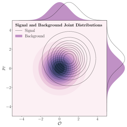
To analytically demonstrate the claims of FORCE, we provide an illustrative Gaussian example. Let denote the normal distribution with mean and variance . Consider two variables and with different distributions for the signal () and background ():
| (13) |
For our numerical analysis, we take , , and all variances to be 1. We fix the background size at 1 million samples and draw the number of signal events to have a signal fraction of . These distributions are shown in Fig. 4 as contour plots. Since the kinematic variable () is drawn independently from the substructure variable (), concatenating these signal and background samples with signal fraction yields a data set with distribution defined by Eq. (3).
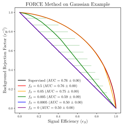
To apply FORCE to this Gaussian example, we use fully connected neural networks with three layers of 100 nodes per layer, training for 10 epochs. The final prediction is taken to be the average over 10 models. We show the decay in statistical power as a function of signal fraction in Fig. 5. As expected, the network behaves optimally in the large signal fraction limit, and converges to a constant random classifier in the no-signal limit.
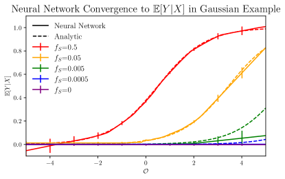
Furthermore, since we know the analytic form for our signal and background distributions, we can construct the conditional expectation formula explicitly:
| (14) |
where the likelihood ratio is:
| (15) |
This allows us to visualize the convergence of the model for various signal fractions, shown in Fig. 6, with optimal performance in the high signal fraction limit and convergence to a constant in the no signal limit.
III Energy Flow Polynomials
Energy flow polynomials (EFPs) are -point correlators on jets that form a discrete linear basis for all infrared and collinear safe (IRC) substructure observables. Diagramatically, they can be represented as loopless multigraphs. For a multigraph , the EFP takes the following form:
| (16) |
Each graph node corresponds to a sum over the energy fraction of the constituents of the jet, while edges correspond to an angular weighting factor between connected particles. A list of the “prime” (i.e. connected graph) EFPs up to degree 3 is shown Table 1.
The definitions for and are context dependent and typically chosen to respect a subgroup of Lorentz symmetry to match the collider detector geometry. For unpolarized hadron colliders, observables are desired to be invariant under beam-direction boosts as well as rotations about the beam axis. Therefore, the particle transverse momentum and rapidity-azimuth (, ) coordinates are used. The energy weighting factor is simply:
| (17) |
For massless particles, as used in our study, a convenient angular weighting factor is:
| (18) |
In the analysis in the main text, we used .
| Degree | Connected Multigraphs |
|
|
|
|
|
|
|
|
|
|
|
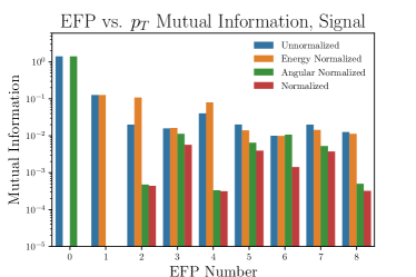
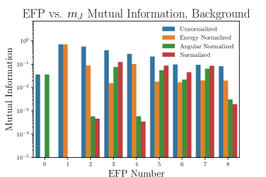
IV Normalization for the Energy Flow Polynomials
As discussed in the main text, to satisfy the factorization structure of the FORCE method, we need to make our EFP observables quasi-scale- and boost-invariant. We can do this by normalizing each polynomial by a factor of
| (19) |
where and are the energy and angular degrees of the polynomial. The reason that yields only quasi-scale and boost invariant observables (and not fully invariant ones) is that the jet radius defines a fixed boundary that does not transform under these transformations. Thus, scaling and/or could either add or subtract particles from the jet, changing the number of terms in the sums.
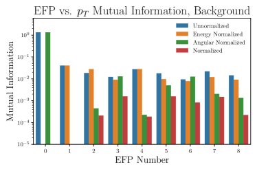
The first term in Eq. (19) equation can be viewed as an energy normalization while the second can be viewed as the angular normalization. To check that these normalization factors yield the desired the factorization structure, we calculate the mutual information between the jet’s and the EFPs with 4 normalization schemes:
-
1.
unnormalized,
-
2.
only energy normalized,
-
3.
only angular normalized, and
-
4.
fully normalized.
The results are shown in the top row of Fig. 7a, for both signal and background events. As expected, full normalization tends to yield the smallest mutual information between the EFPs and jet among all the normalization schemes, motivating its use as a factorized observable for the FORCE method.
One additional benefit of full normalization is that the FORCE model becomes less correlated from jet mass, as shown in the bottom row of Fig. 7a. Jet mass itself corresponds to the unnormalized EFP 2, and after angular normalization, this EFP has minimal correlation with jet mass as expected. While the other EFPs retain some correlation with jet mass even after full normalization, it is a small effect that does not result in excessive mass sculpting in our case study.

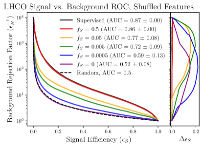
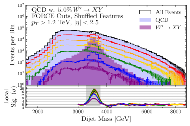
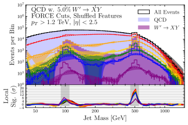
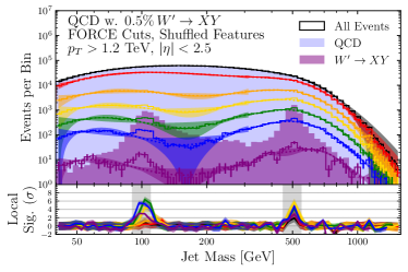
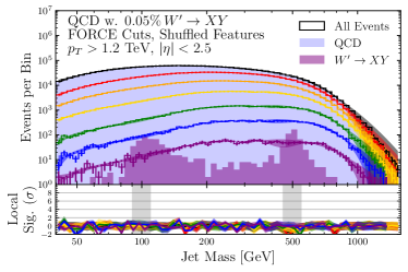
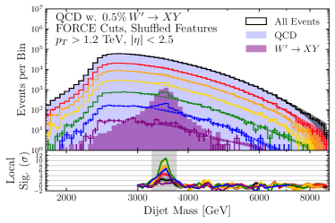
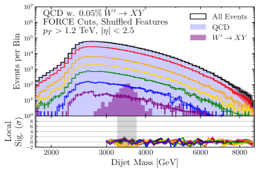
V Shuffled Features for Factorized Objects in the LHC Olympics
As noted in the main text, the learned model did not converge to a constant function, unlike the prediction from the conditional expectation in Eq. (6). This implies that there is some non-factorized dependence in our realistic case study that is being learned and exploited by the model.
To demonstrate an idealized use case, we construct a dataset that follows Eq. (3) exactly to check that it has the expected behavior. For the signal and background separately, we create joint distributions as the product of its marginals:
| (20) | ||||
| (21) |
We call these “shuffled” datasets, since they correspond to independently drawing and substructure variables without replacement. To create the full dataset with data points drawn from the factorized joint distribution,
| (22) |
we draw samples from and samples from , with , and concatenate these draws.
The signal versus background discrimination results for the shuffled dataset are shown in Fig. 8. We see the expected behavior in both the no-signal and high-signal case, with no-signal functioning as a random classifier and the high-signal limit approaching optimal discrimination.
For completeness, we repeat the analysis from Fig. 2 with the jet and dijet mass bump hunt results, but for three different values of the signal fraction. The results for the original samples are shown in Fig. 9a, while the results for the shuffled sample are shown in Fig. 10a. We see that shuffling does not change the qualitative features of these plots, implying that the original samples obeyed factorization sufficiently well for FORCE to yield trustable results.