DynMF: Neural Motion Factorization
for Real-time Dynamic View Synthesis with 3D Gaussian Splatting

Abstract

Accurately and efficiently modeling dynamic scenes and motions is considered so challenging a task due to temporal dynamics and motion complexity. To address these challenges, we propose DynMF, a compact and efficient representation that decomposes a dynamic scene into a few neural trajectories. We argue that the per-point motions of a dynamic scene can be decomposed into a small set of explicit or learned trajectories. Our carefully designed neural framework consisting of a tiny set of learned basis queried only in time allows for rendering speed similar to 3D Gaussian Splatting, surpassing 120 FPS, while at the same time, requiring only double the storage compared to static scenes. Our neural representation adequately constrains the inherently underconstrained motion field of a dynamic scene leading to effective and fast optimization. This is done by biding each point to motion coefficients that enforce the per-point sharing of basis trajectories. By carefully applying a sparsity loss to the motion coefficients, we are able to disentangle the motions that comprise the scene, independently control them, and generate novel motion combinations that have never been seen before. We can reach state-of-the-art render quality within just 5 minutes of training and in less than half an hour, we can synthesize novel views of dynamic scenes with superior photorealistic quality. Our representation is interpretable, efficient, and expressive enough to offer real-time view synthesis of complex dynamic scene motions, in monocular and multi-view scenarios.

1 Introduction

The generation of a photorealistic representation, from an unseen point of view, also known as Novel View Synthesis, poses a long-standing challenge to the graphics and computer vision community. While there exist early methods that tackle this problem, both for static [17, 28] and dynamic scenes [10, 18], neural rendering has received widespread attention only after the pioneering work of NeRF [21]. Following the latter, numerous methods have contributed to the static neural rendering problem, by tackling aliasing problems [4, 5], generalizing to larger scales [44, 32, 6], and to new scenes [36] and increasing efficiency and rendering speed [30, 12, 22, 8, 9].

While the advance in novel view synthesis of static scenes has been rapid, the high-quality efficient photorealistic rendering of dynamic scenes still poses a vivid challenge to the aforementioned communities. The numerous applications, including but not limited to augmented reality/virtual reality (AR/VR), robotics, self-driving, content creation, and controllable 3D primitives for use in video games or the meta-verse, have kept the interest in expressive dynamic novel view synthesis to high levels. From recent pioneers of neural dynamic rendering [26, 19] to the latest [20], numerous efforts have been made to drastically improve this field and bring it one step closer to real applications. Altering the scene representation from MLPs [26, 19] to grids [35], or other decompositions [13, 3, 27, 7] for efficiency and faster training, proposing expressive deformation representations [1, 29, 24, 23, 41] or using template guided methods [39, 47] are just a few of the approaches taken the last few years.

Despite all these approaches, dynamic novel view synthesis is still a challenging problem, with quick training, real-time rendering, and highly accurate and visually appealing novel views yet to be achieved. Dynamic scenes require disambiguating displacements, and disentangling overlapping motions, especially due to non-rigid objects and monocular captured scenes that make this even more challenging. We propose a compact, simple, and expressive neural representation that can adequately tackle the previous challenges. Namely, we propose a sparse trajectory decomposition of all the motions in the dynamic scene, to accurately represent displacements, overlapping and non-rigid motions. Our framework is strategically designed to offer extremely fast training and real-time rendering of a dynamic scene. Specifically, we argue that a scene consists of only a few basis trajectories (even less than 10) and every point/motion shall be adequately mapped to one of them or a linear combination of them. The basis motions are learned through a tiny MLP queried only in time leading to superfast convergence during training (less than 5 minutes for photorealistic results, and half an hour for superior to the state-of-the-art ) and superfast rendering during inference (higher than 120 FPS for resolutions of 1K). By strategically constraining an inherently underconstrained problem in this way, we are able to successfully optimize for cases with very few correspondences (e.g. monocular videos). Simultaneously, being able to efficiently factorize all the motions of a dynamic scene into a few basis trajectories, allows us in turn, to control them, enable or disable them, opening a road to applications like video editing, scene controllability, interactive and real-time motion control, efficient animation and so on.

In this work, we present DynMF (DYNamic neural Motion Factorization). The contributions of this paper can be summarized as follows:

• We manage to expressively model scene element deformation of complex dynamics, through a simple and interpretable framework. Our method enables robust per-point tracking, overcoming displacement ambiguities, overlappings, and non-rigid complex motions. It also enables the synthesis of novel motion scenes, that have never been seen before through disentangling motion and carefully enforcing sparsity.

• DynMF is extremely efficient. The carefully designed time-only queried MLP allows for training in less than 30 minutes while the rendering speed remains comparable to 3D Gaussian Splatting [15]. This allows for real-time rendering of static and dynamic scenes.

• We propose a neural representation that can effectively constrain the ill-posed nature of dynamic 3D motion reconstruction and requires no prior knowledge of the scene. Our method achieves high-quality real-time dynamic rendering, while significantly surpassing the state-of-the-art benchmarks on the D-NeRF dataset and achieving comparable results on the real-scene datasets.

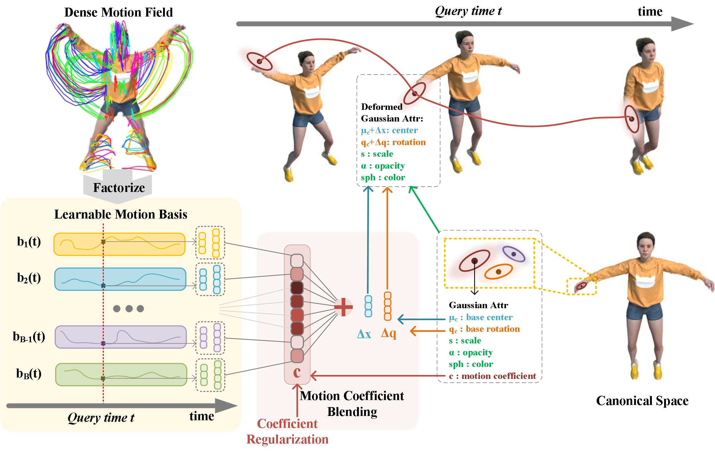
Figure 2: Overview of DynMF. The underlying dense motion field (left-top) of a dynamic scene is factorized into a set of globally shared learnable motion basis (left-bottom) and their motion coefficients stored on each Gaussian (right-bottom). Given a query time $t$, the deformation can be efficiently computed via a single global forward of the motion basis and the motion coefficient blending (middle-bottom) to recover the deformed scene (top-right).

2 Related Work

Dynamic Neural Rendering: The recent works on NeRF [21] and D-NeRF [26] both proposing a coordinate-based neural network, the former for querying points on a ray to produce color and density for static scenes and the latter to model the deformation field and create an expressive mapping between a canonical space and a dynamic scene, have provoked an explosion of interest in the field of static and dynamic novel view synthesis. On the dynamic side, we can distinguish three main approaches: (i) methods that construct a deformation field to warp a canonical space to every timestep [26, 23, 24, 37, 41] (ii) methods that try to model the dynamic scene as a whole, implicitly or explicitly [13, 7, 19, 35, 3] and (iii) point-based methods [1, 45, 20] that due to dense correspondence over time between frames and due to their Lagrangian representation, can achieve consistent and expressive dynamic scene modeling. We relax that latter restriction by proposing a point-based method that can construct an efficient and expressive deformation field, explicit or learned, without the need for dense correspondences through multiple frames or multiple views.

Motion Factorization: Decomposing a complex motion field into a linear combination of basis trajectories has been a well-established approach from Mathematics and Physics to Signal Processing and Computer Vision. In the latter field, [2] has proposed an explicit trajectory-based factorization for non-rigid structure for motion in which every point in space can be linearly expressed by a combination of DCT trajectories. Clustering trajectories into a small number of subspaces has been argued by [16] for the same task, while [48] has explored trajectories’ convolutional structure. Following [2, 33], [34] has also exploited DCT trajectory basis for the task of dynamic novel view synthesis, by predicting a per-point trajectory using an MLP to acquire the DCT coefficients. Our method argues that a per-point trajectory is redundant and can only work given a lot of correspondences or strong regularization. In fact, [34] leverages optical flow in their optimization scheme.

Dynamic 3D Gaussians and Concurrent work: Parallel to our work there have been four other concurrent works that utilize 3D Gaussian Splatting for Dynamic Neural Rendering. First, Dynamic 3D Gaussians [20] uses online training and rigidity losses to synthesize novel views timestamp per timestamp. For their method to work, though, they require multiple cameras and depth information to reconstruct the first frame, while at the same time, their method cannot handle the appearance of new objects in the scene. DynMF works on scenes captured by a single monocular camera and with random initialization incorporating information from all frames all at once. [42] uses a coordinate-based MLP similarly to D-NeRF [26] as a deformation field. This approach may be slow and inefficient because it requires querying MLP for each gaussian. Our method is extremely time-efficient and does not significantly depend on the number of Gaussians. [43] is optimizing 4D primitives to treat the spacetime as an entirety, while [40] is connecting adjacent Gaussians via a HexPlane to model position and shape deformations. Our neural representation is simple and interpretable by decomposing all the complex motions of a dynamic scene into very few neural trajectories.

3 Method

We propose a compact representation that is shared across all points and models the dynamics of a scene. We argue that every scene is comprised of a limited fixed number of trajectories. In other words, we can model a 3D dynamic scene by a few universal trajectories that are shared between the 3D world points. In this section, we first formally present the representation of our motion field, DynMF, that is able to model the 3D dynamic scene and synthesize novel views (Section 3.1). In Section 3.2 we review the framework in which we bundle our motion field representation to efficiently learn the 3D world, namely 3D Gaussian Splatting, while in Section 3.3 we present the optimization and regularization details.

3.1 Motion Representation Fields

Let a dynamic scene be represented by a point cloud of N points $\bm{x}\in\mathbb{R}^{N\times 3}$. We assume a sequence of frames in the interval $t\in[0,T]$, taken from one or multiple viewpoints. Assuming a canonical space $\bm{x_{c}}\in\mathbb{R}^{N\times 3}$ we define $B$ trajectories $\bm{b}_{j}(t):[0,T]\rightarrow\mathbb{R}^{3}$ such that for every $\bm{x}\in\mathbb{R}^{3}$ we have:

$$\bm{x}(t)=\bm{x_{c}}+\sum_{j=1}^{B}c_{j}\bm{b}_{j}(t)$$ (1)

where $c_{j}\in\mathbb{R}^{N\times 3}$ are the motion coefficients for each point, and $\bm{x}(t)$ are the points’ motion trajectories across the entire sequence. We let the basis be shared across all points arguing that the dynamic motions of a scene can be explicitly represented by a linear combination of B trajectories. This factorization problem becomes an overconstrained low-rank factorization as soon as the number of points $N$ exceeds the number of basis trajectories $B$. This is easy to see if we discretize the time into $T$ timestamps and write only the x-coordinates as matrices $\bm{X},\bm{X_{c}}\in{\mathbb{R}}^{N\times T}$

$${\bm{X}}={\bm{X}_{c}}+\bm{C}\cdot\bm{B}$$ (2)

with $\bm{C}\in{\mathbb{R}}^{N\times B}$ and $\bm{B}\in{\mathbb{R}}^{B\times T}$ and $B$ much lower than $N$ or $T$.

We reason that given enough correspondences and expressive basis functions, we can jointly learn the canonical space and each point’s motion by reconstructing its trajectory across the whole sequence. Sharing the basis across all points enables the representation to produce physically plausible motions that stay consistent across all frames.

If we let

$$\bm{b}_{j}(t)=\left\{\begin{array}[]{ll}cos\left(\frac{2\pi j}{T}t\right),&\text{if j is odd}\\ sin\left(\frac{2\pi j}{T}t\right),&\text{if j is even}\\ \end{array}\right.$$ (3)

the factorization is equivalent to modeling the dynamic motion trajectories of a scene with Fourier series. While Fourier bases are global approximators for any trajectories and have been shown to be a compact representation for dynamic scenes with deformations [38, 46], we argue that a learned basis will be smoother and more expressive for this task (see Section 4.5 for ablations). Thus, we let:

$$\mathbf{b}_{j}(t)=\textbf{MLP}\left(\frac{t}{T};w_{j}\right)$$ (4)

be a small multilayer perceptron queried only over time. While the learned functions are not strictly a basis, we empirically observe that they span a large enough space that covers the variation of deformations in the scene. Overall, we propose a representation of the dynamic scene in which a small MLP predicts along all timestamps a few compact basis trajectories, and all the points in the scene are bound to linearly choose between these to model their motion across time.

3.2 3D Gaussian Splatting

We choose to bind the aforementioned representation with 3D Gaussian Splatting [15]. The latter is an explicit 3D scene representation used for efficient and expressive neural rendering.

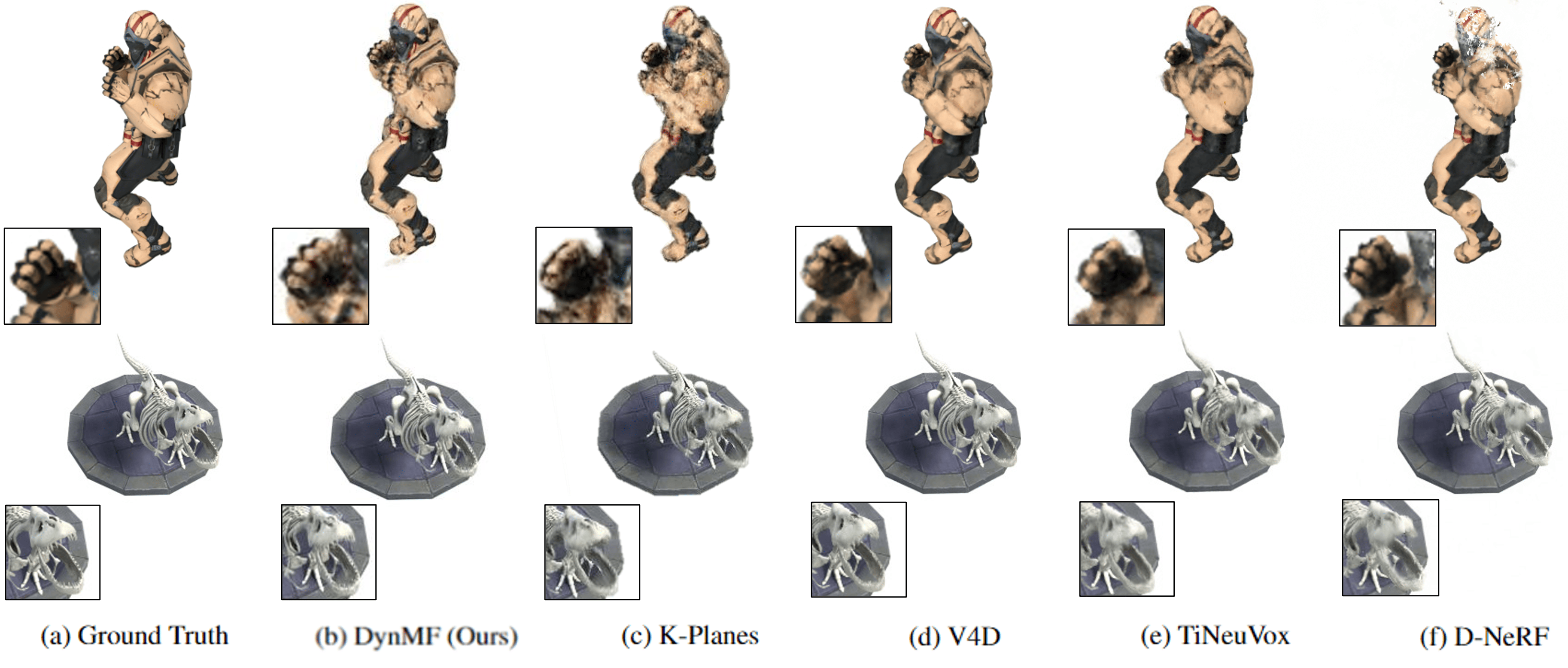
Figure 3: Qualitative comparison on the D-NeRF dataset between our method and the state-of-the-art.

Static 3D Gaussians: The 3D space is described in the form of a point cloud by a set of 3D Gaussians which are defined by a mean value $\bm{\mu}$ and a 3D covariance matrix $\bm{\varSigma}$ in the world space. The influence of one Gaussian with parameters $(\bm{\mu},\bm{\varSigma})$ on a given spatial position $\bm{x}\in\mathbb{R}^{3}$ is defined by:

$$f(\bm{x}|\bm{\mu},\bm{\varSigma})=e^{-\frac{1}{2}\left(\bm{x}-\bm{\mu}\right)^{T}\bm{\varSigma}^{-1}\left(\bm{x}-\bm{\mu}\right)}$$ (5)

The anisotropic full 3D covariance matrix is decomposed into a rotation matrix $\bm{R}$ and a scaling matrix $\bm{S}$:

$$\bm{\varSigma}=\bm{R}\bm{S}\bm{S}^{T}\bm{R}^{T}.$$ (6)

To render the 3D Gaussians in a differentiable manner [15] Gaussians are splatted on the image plane by approximating the 2D means and covariances from the 3D ones. The center of the Gaussian is splatted using the standard point rendering formula:

$$\bm{\mu}^{2D}=\bm{K}\frac{\bm{E}\bm{\mu}}{\bm{E}\bm{\mu}_{z}}$$ (7)

where $K,E$ are the intrinsic projection matrix and the world-to-camera extrinsic matrix, respectively. The 3D covariance matrix is splatted into 2D using [49]:

$$\bm{\varSigma}^{2D}=\bm{J}\bm{E}\bm{\varSigma}\bm{E}^{T}\bm{J}^{T}$$ (8)

where $\bm{J}$ is the Jacobian of the point projection formula in 7. Finally, the color of a specific pixel $p$ can be computed as:

$$C_{p}=\sum_{i=1}^{N}c_{i}\alpha_{i}f\left(p|\bm{\mu}^{2D},\bm{\varSigma}^{2D}\right)\prod_{j=1}^{i-1}\left(1-\alpha_{j}f\left(p|\bm{\mu}^{2D},\bm{\varSigma}^{2D}\right)\right)$$ (9)

where $c_{i},\alpha_{i}$ are the color and opacity, bound with each 3D Gaussian. Overall, each Gaussian is characterized by the following attributes: i. a center mean $\bm{\mu}\in\mathbb{R}^{3}$, ii. a scale factor $\bm{s}\in\mathbb{R}^{3}$ and a rotation $\bm{R}\in SO(3)$ that we parametrize with a unit quaternion in ${\mathbb{S}}^{3}$, iii. an opacity logit $\alpha\in\mathbb{R}$ and iv. each color defined by spherical harmonics coefficients $\bm{c}_{R,G,B}\in\mathbb{R}^{(L+1)^{2}}$ where $L$ is the maximum degree of spherical harmonics.

Dynamic 3D Gaussians: The previous framework is capable of modeling efficiently and expressively a 3D static scene. To use it for representing a 3D dynamic scene we propose the following:

1. Substituting the mean $\bm{\mu}$ with $\bm{\mu}(t)$. The mean’s trajectory $\bm{\mu}(t)$ will be decomposed according to Equations 1 and 2:

   $$\bm{\mu}(t)=\bm{\mu}_{c}+\sum_{j=1}^{B}c_{j}\bm{b}^{\mu}_{j}(t)$$ (10)

   where $\bm{\mu}_{c}\in\mathbb{R}^{3}$ is the mean center of the Gaussian in the canonical space and $\bm{c}=\left[c_{j}\right]_{j=1,\dots,B}$ the motion coefficients, both stored as learned parameters per Gaussian.

2. Substituting the rotation quaternion $\bm{q}$ with $\bm{q}(t)$. The rotation quaternion will be decomposed similarly:

   $$\bm{q}(t)=\bm{q}_{c}+\sum_{j=1}^{B}c_{j}\bm{b}^{R}_{j}(t)$$ (11)

   where $\bm{q}_{c}\in\mathbb{R}^{4}$ is the rotation quaternion of the Gaussian in the canonical space stored as learned parameter per Gaussian. Note that the motion coefficients are shared for both the translational and rotational decompositions.

3. Keeping density and spherical harmonic coefficients of each Gaussian fixed along time. The basis functions $\{\bm{b}_{j}^{\mu}(t)\}$ and $\{\bm{b}_{j}^{R}(t)\}$ are chosen according to Equations 3 and 4.

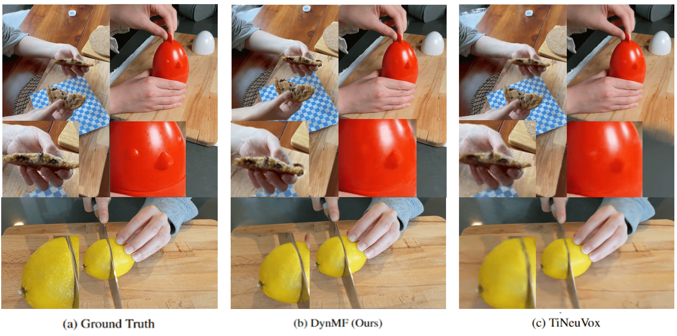
Figure 4: Qualitative comparison on the HyperNeRF dataset.

We argue that the proposed framework is a compact and expressive representation of 3D dynamic scenes that consist of multiple decoupled and complicated motions. By sharing the basis functions between Gaussians, we constrain neighbor Gaussians and rigid areas to choose similar trajectories, softly enforcing locality and rigidity a priori. At the same time, sharing the motion coefficients and keeping the number of basis trajectories low, dramatically softens the restrains of this ill-posed optimization problem. The efficient design of the basis functions retains the rendering speed at the same levels as with the original Gaussian Splatting, enabling real-time rendering not only for static scenes but for dynamic as well.

3.3 Optimization Framework

Regularization: The optimization process will naturally converge to a linear combination of all basis functions per Gaussian. Furthermore, Gaussians tend to move, even if they are part of the background as long as they do not harm the photometric accuracy with their movement (e.g. Gaussians moving on a white wall). While the former is desirable and increases expressivity, the latter harms the representation’s interpretability since the basis functions are forced to learn trajectories for unnecessary movements. To solve this problem, we add an L1 regularization loss on the motion coefficients to penalize unnecessary choices of basis functions and thus, apparent but nonexistent movements:

$$\mathcal{L}_{1}=\frac{1}{NB}\sum_{i=1}^{N}\sum_{j=1}^{B}|c_{ij}|$$ (12)

Sparsity: Enforcing sparsity between the trajectories is more challenging. While $\mathcal{L}_{1}$ loss is supposed to encourage sparsity by increasing competition between the weights, we observed that the moving Gaussians kept choosing a linear combination of the trajectories with just smaller weights. To solve this we added a new stronger loss that explicitly forces each Gaussian to choose only very few trajectories:

$$\mathcal{L}_{s}=\frac{1}{NB}\sum_{i=1}^{N}\sum_{j=1}^{B}\frac{|c_{j}|}{\displaystyle\max_{j}|c_{j}|}$$ (13)

With a strong enough loss weight, this quantity enforces strict sparsity which can lead to dynamic motion decoupling and novel motion synthesis.

Rigidity: Our representation naturally encourages rigidity between the Gaussians. Restraining the number of trajectories drives nearby points to choose the same trajectory. Furthermore, when a Gaussian is split or densified into a new one, we choose to copy the motion coefficients to the new Gaussian, to naturally enforce rigidity to the scene. We experiment with a simple rigid loss:

$$\mathcal{L}_{r}=\frac{1}{Nk}\sum_{i=1}^{N}\sum_{j\in knn_{i;k}}w_{ij}\lVert\bm{c}_{i}-\bm{c}_{j}\rVert_{2},$$ (14)

where the set of $j$ Gaussians choose the k-nearest neighbours of $i$ and weight the loss, similar to [20], by an isotropic Gaussian weighting factor per Gaussian pair $w_{ij}=exp\left(-\lambda_{w}\lVert\bm{\mu}_{i}(t^{*})-\bm{\mu}_{j}(t^{*})\rVert_{2}^{2}\right)$. We demonstrate that $\mathcal{L}_{r}$ does not further increase the rendering quality of the scene, solidifying our intuition that our motion representation is inherently rigid, given a small number of trajectories. For ablations on the optimization scheme, please refer to the Supplementary material.

Model	PSNR(dB) $\uparrow$	SSIM $\uparrow$	LPIPS $\downarrow$	Time $\downarrow$	FPS $\uparrow$
D-NeRF [26]	29.67	0.953	0.06	$15.9\mathrm{hours}$	$0.1$
K-Planes [13]	31.61	0.970	$-$	$52\mathrm{mins}$	0.1
TiNeuVox [11]	32.67	0.970	0.04	$\mathbf{\mathrm{21m}}$	1.5
V4D [14]	33.72	0.980	–	$4.9\mathrm{hours}$	$2$
DynMF (Ours)	$\mathbf{36.89}$	$\mathbf{0.983}$	$\mathbf{0.02}$	$30\mathrm{mins}$	$\mathbf{>300}$

Table 1: Quantitative results on synthetic monocular D-NeRF dataset. The rendering resolution is 400×400.

4 Experiments

4.1 Experimental Setup

In this section, we present the results of our method for three different scenarios; synthetic-scene monocular, real-scene monocular and real-scene multi-view.

D-NeRF [26] is a monocular synthetic dataset with a total of 8 rigid and non-rigid scenes. Each scene contains dynamic frames, ranging from 50 to 200 in number and on a unique timestamp. The camera pose for each timestamp is also different. HyperNeRF [24] is a monocular dataset on real-scenes. It consists of many scenes of different real objects and actions with one or two cameras that are moving over time. We choose one rigid and three highly non-rigid scenes to test the method’s efficiency in challenging cases like these. The four scenes are the ‘3d-printer’, ‘split-cookie’, ‘cut-lemon’, and ‘chicken’. DyNeRF [19] dataset is a real-world dataset consisting of 6 very challenging dynamic scenes. The scenes are captured by 15-20 static cameras in total that share a common time. The scenes consist of long highly non-rigid motions and dynamic opacity (e.g. flame or smoke).

Model	PSNR(dB) $\uparrow$	SSIM $\uparrow$	LPIPS $\downarrow$	Time $\downarrow$	FPS $\uparrow$
HyperNeRF [24]	28.5	–	0.19	$52\mathrm{mins}$	0.1
TiNeuVox [11]	26.87	0.75	0.37	$\mathrm{50m}$	0.5
DynMF (Ours)	28.9	0.84	0.21	30mins	$\mathbf{>120}$

Table 2: Quantitative results on real-scene monocular HyperNeRF dataset. Results for the following scenes: chicken, split-cookies, cut-lemons, and 3d-printer. The rendering resolution is 960×536.

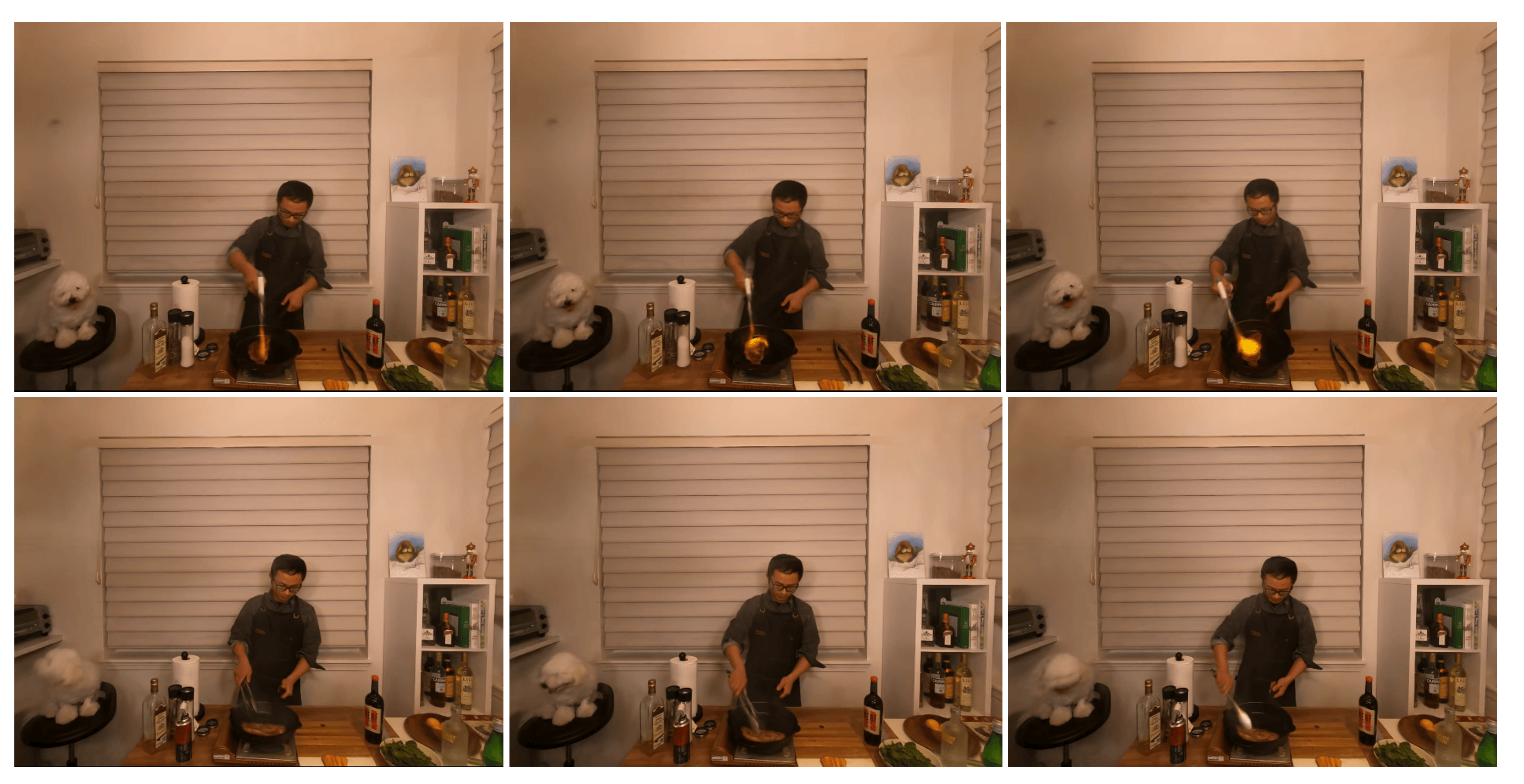
Figure 5: Novel view synthesis of DynMF. The figure shows selected frames from different time frames for the scenes ’flame-steak’ and ’flame-steak’.

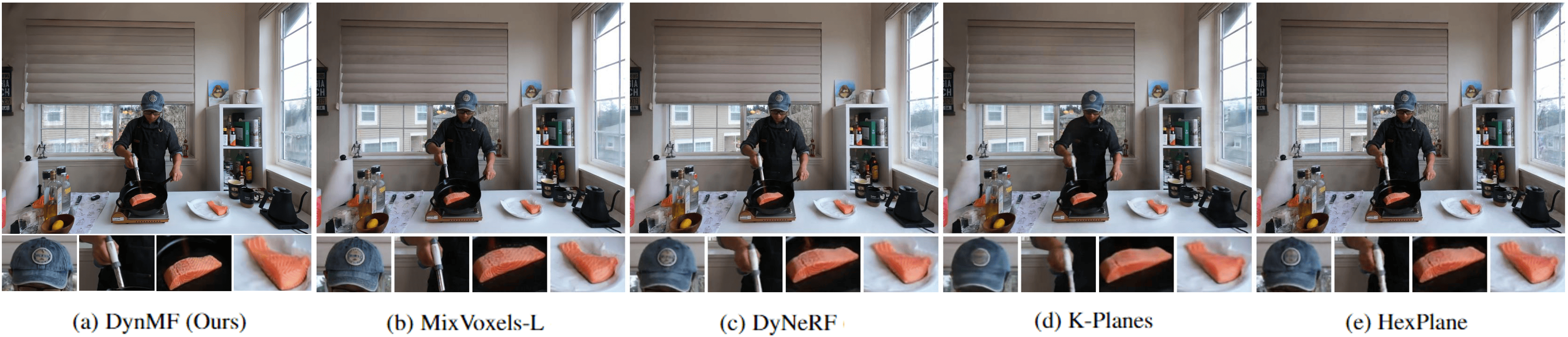
Figure 6: Qualitative comparison on the DyNeRF dataset between our method and the state-of-the-art.

4.2 Implementation Details

The motion representation field is implemented in PyTorch [25], while we keep the differentiable Gaussian rasterization implemented by 3D-GS [15]. The MLP consists of 3 linear layers of 256-width with 2 final layers producing $(B,3)$ and $(B,4)$ numbers that constitute the displacement and quaternion correction per trajectory for a specific time. For the number of trajectories $B$, we choose $10$ for D-NeRF and HyperNeRF and $16$ for DyNeRF dataset. We apply positional encoding to the input of the MLP, which has been shown to be fundamental for good performance [21, 31]. Since the network is not coordinate-based and is solely based on time, a high-frequency input is needed for producing expressive trajectories for the dynamic scenes. We choose 26 frequencies to encode time. See Section 4.5 for ablations on the number of trajectories and position encoding of time. For training, we conduct training for a total of 30k iterations, while enabling the training of the basis functions and motion coefficients only after the first 3k iterations. All the parameters are kept the same with respect to 3D-GS while the learning rate of the basis is exponentially decaying from 8e-4 to 8e-6 and the learning rate of the coefficients is kept at 8e-3. 2k Gaussians’ means are randomly initialized around the center of the scene for all datasets, solidifying the stability and generalizability of our representation.

Model	PSNR(dB) $\uparrow$	SSIM $\uparrow$	LPIPS $\downarrow$	Time $\downarrow$	FPS $\uparrow$
DyNeRF [19]	29.58	-	$\mathbf{0.08}$	$1344\mathrm{hours}$	$0.015$
MixVoxels-L [35]	30.80	0.96	-	$1.3\mathrm{hours}$	$16.7$
K-Planes [13]	31.63	0.964	-	$1.8\mathrm{hours}$	0.15
Hexplane [7]	$\mathbf{32.22}$	$\mathbf{0.98}$	0.09	$12\mathrm{hours}$	0.09
DynMF (Ours)	31.70	0.96	0.11	$\mathbf{0.8hours}$	$\mathbf{>130}$

Table 3: Quantitative results on real-scene multi-view DyNeRF dataset. The rendering resolution is $1386\times 1014$.

4.3 Results

Results on Synthetic data: A quantitative evaluation of the D-NeRF synthetic Dataset is presented in Table 1. Our method surpasses all state-of-the-art methods by a significant gap in all metrics. This confirms that DynMF is an adequate representation of rigid, decoupled, and non-rigid/deformable motion as well. Regarding speed, our method achieves state-of-the-art results in only 10 minutes of training, while after half an hour it synthesizes most of the dynamic scenes almost perfectly. The FPS rate for $400x400$ images reaches more than 300FPS confirming the carefully designed representation in terms of efficiency, achieving real-time dynamic novel view synthesis. Qualitative comparisons can be seen in Figures 3.

Results on Real data: DynMF seems to achieve state-of-the-art results on the HyperNeRF and DyNeRF datasets as well, as shown in Tables 2 and 3. These datasets consist of very challenging non-rigid motions and semi-transparent areas that the representation of motion factorization can adequately and efficiently express. Again, time-wise our method allows for real-time dynamic rendering even on scenes of high resolution like DyNeRF (i.e. $1280\times 1080$). For a per-scene evaluation of all three datasets and for more qualitative results, please refer to the supplementary material.

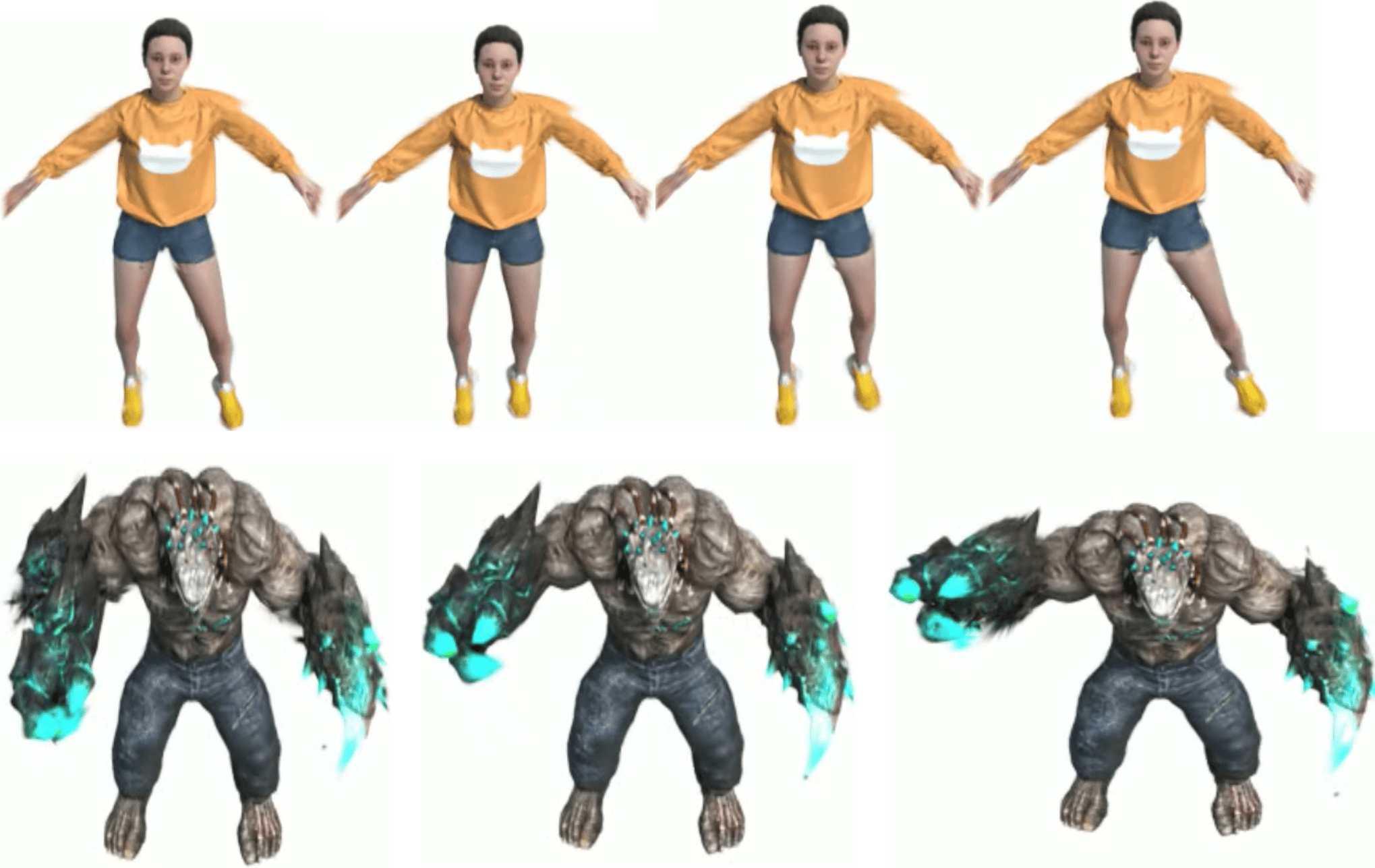
Figure 7: Demonstration of the decomposition capabilities of our representation. Independent movement of the right foot and the left hand of the ‘Jumpingjacks’ and ‘Mutant’ scenes respectively.

Model (B, F)	Mutant	Steak	Model (B, F)	Mutant	Steak
DynMF (1,32)	29.75	28.85	DynMF (10,1)	39.08	29.32
DynMF (4,32)	39.98	30.34	DynMF (10,6)	39.61	29.59
DynMF (10,32)	40.79	31.57	DynMF (10,16)	40.50	31.29
DynMF (20,32)	40.76	31.03	DynMF (10,32)	40.79	31.57
DynMF (50,32)	40.53	30.99	DynMF (10,60)	40.53	29.80

Table 4: Ablation study on the number $B$ of the motion trajectories and the frequencies $F$ of the positional encoding applied on time. PSNR is used as the metric on the ‘Mutant’ scene from the D-NeRF dataset and the ‘Flame-steak’ scene from the DyNeRF dataset.

4.4 Motion Decomposition

A key component of our proposed representation is its ability to explicitly decompose each dynamic scene to its core independent motions. Specifically, by applying the sparsity loss described in Section 3.3, we enforce each Gaussian to choose only one of the few trajectories available. This design combined with the inherent rigid property of our representation drives all nearby Gaussians to choose the same and only trajectory. This strongly increases the controllability of the dynamic scene, by disentangling motions, allowing for novel scene creation, interactively choosing which part of the scene is moving, and so on. Figure 7 shows two examples of motion control in two synthetic scenes. Please, refer to the supplementary video for a deeper understanding of the motion decomposition possibilities that our representation enables

4.5 Ablation Studies

Time encoding and Number of trajectories: The number of trajectories, $B$ is the most important hyperparameter of DynMF, for it is the one that decides in what detail will the scene be modeled. In parallel, the positional encoding on time proved to be important as well, with notoriously high frequencies, $F$, needed for state-of-the-art results. Table 4 shows experiments on multiple combinations of $(F,B)$. We can see that both synthetic and real scenes can be adequately modeled by very few trajectories while adding more only subtly increases the performance. At the same time, while encoding time is not vital for satisfactory rendering, mapping it to higher frequencies provides the mean for more expressive trajectories by the small MLP. Please, refer to the Supplementary material for qualitative comparisons for different values of $B$ and $F$.

Fourier Series: Table 5 shows results on two different scenes (mutant from D-NeRF and flame-steak from DyNeRF) in the case of a non-learned motion and rotation base, in this case the Fourier Series. We conducted a few experiments with the basis functions following Equation 3 and we varied the number of frequencies the basis could incorporate. We observe that the Fourier series can satisfactorily express the motion field of a dynamic scene but is not expressive and smooth enough to decode the details of complicated scenes. To the best of our knowledge, this is the first totally explicit dynamic scene representation, comprised of Gaussians and Fourier series. In supplementary material, we further investigate the reasons why the Fourier basis is not expressive enough.

Model	Mutant	Steak
DynMF (Learned Basis)	40.79	31.57
DynMF (Fourier 10)	33.17	28.95
DynMF (Fourier 20)	35.21	27.18
DynMF (Fourier 50)	33.87	23.42
DynMF (Fourier 100)	21.12	19.15

Table 5: Ablation study on the basis function. PSNR is used as the metric on the ‘Mutant’ scene from the D-NeRF dataset and the ‘Flame-steak’ scene from the DyNeRF dataset.

5 Conclusion & Future Work

In this work, we have introduced, DynMF, a motion factorization framework that enables real-time rendering of dynamic scenes. The carefully designed representation of a small MLP queried only by time allows for training convergence in half an hour and for a rendering speed of more than 120 FPS. At the same time, the shared motion basis scheme supports inherently the locality and rigidity of the motions and allows for state-of-the-art rendering quality from novel views. Last but not least, the motion decomposition properties allow us to dive deeper into the structure of the scene and create novel instances by independently enabling and disabling motions on the scene. For future work, we believe that DynMF is potentially a good representation for efficient and accurate tracking as well. While the motion factorization framework along with the 3D Gaussian splatting gives the opportunity for detailed and expressive novel view synthesis of dynamic scenes, it is by itself constructed in a way to allow tracking of all the points on the scene at every time.

Supplementary Material

PSNR $\uparrow$
DynMF		Hell Warrior	Mutant	Hook	Balls	Lego	T-Rex	Stand Up	Jumping Jacks		Mean
B=10 w $\mathcal{L}_{decomp}$		31.60	40.01	29.89	41.05	24.49	32.93	38.52	33.61		34.01
B=64 w $\mathcal{L}_{decomp}$		34.70	40.16	31.83	42.14	25.58	33.96	38.97	35.53		35.36
B=10 w $\mathcal{L}_{1}$		36.60	41.00	31.30	41.01	25.27	35.10	41.16	35.75		35.90
B=64 w $\mathcal{L}_{1}$		37.51	41.68	33.91	41.95	25.51	35.82	41.00	37.74		36.89
B=10 w $\mathcal{L}_{rigid}$		36.10	40.11	32.01	39.85	25.20	34.89	40.50	34.74		35.43
B=64 w $\mathcal{L}_{rigid}$		37.10	40.64	33.15	41.41	25.31	34.99	40.79	37.41		36.35
B=10 w no Losses		36.51	40.79	31.36	40.03	25.29	35.08	41.10	35.74		35.74
B=64 w no Losses		37.31	41.32	33.94	41.95	25.37	35.19	41.16	38.04		36.79

Table 6: Ablation study on the $\mathcal{L}_{1}$ regularization loss, on the $\mathcal{L}_{decomp}$ sparsity loss and on the $\mathcal{L}_{r}igid$ rigid loss. $B$ refers to the number of basis trajectories for the scene.

In this part, we present a few more important ablation studies that are essential for the understanding of our method’s functionality. First and foremost, this section is accompanied by a video presentation that briefly explains the methodology of our framework and demonstrates a plethora of dynamic rendering results and ablations. This summarizes and demonstrates our results in rendering, tracking, and decomposition in the best possible way. Next, we offer a series of ablations studies. We show a few visual comparisons between using or not the $\mathcal{L}_{1}$ loss regularization on the motion coefficients, we present a big ablation on the usage of each one of the three aforementioned losses, and we finally visualize the 10 basis trajectories a scene is comprised of, in the case where they are linearly combined to produce motions, independently combine to produce motions (sparsity) or explicitly defined by the Fourier series. At the end of the supplementary material, we demonstrate a few more rendering results and present analytic quantitative results for every scene on each dataset for the three main metrics, PSNR, SSIM, and LPIPS.

6 Ablations

$\mathcal{L}_{1}$ Loss Regularization: As described in the main paper, Gaussians tend to choose a trajectory and move, even if they are part of the background. This is feasible without hurting the photometric accuracy. We regularize the motion coefficients to penalize unnecessary movements. Figure 8 and 9 show some qualitative comparisons between enforcing or not an $\mathcal{L}_{1}$ regularization. We observe that the $\mathcal{L}_{1}$ loss is enough to enforce points on the background to remain static during the process.

Rigid Loss: We strongly believe our method encourages locality and rigidity properties between points in the dynamic scene, given a small but adequate number of basis trajectories. We conduct experiments with and without the rigid loss and observe that the latter offers no additional expressiveness in the rendering quality of the dynamic scenes, while at the same time, it severely increases the training time especially when the number of Guassians is substantial. For the quantitative results refer to Table 6.

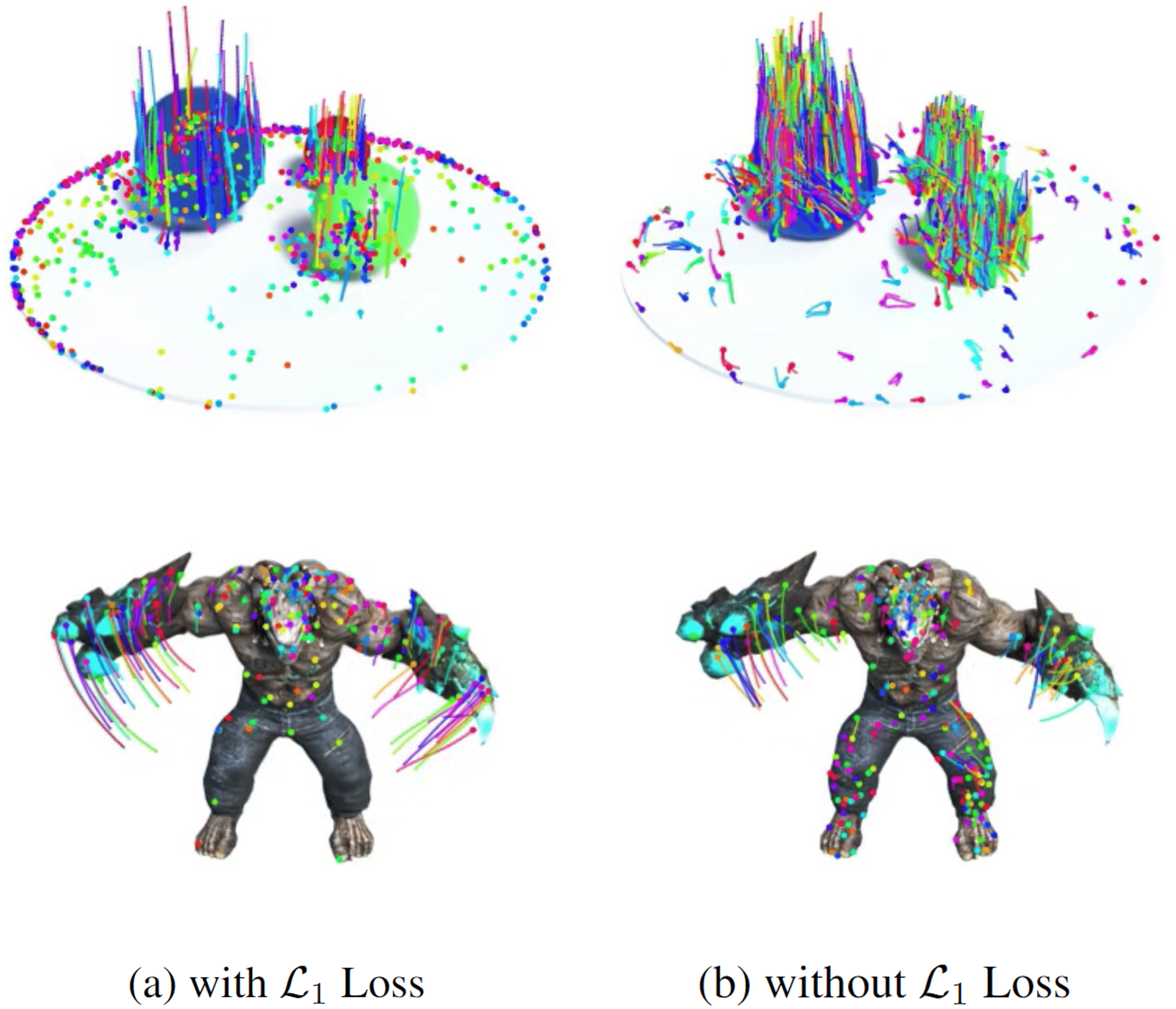
Figure 8: Qualitative comparison between using or not the $\mathcal{L}_{1}$ loss for regularizing the motion coefficients of each Gaussian. Results for the D-NeRF dataset.

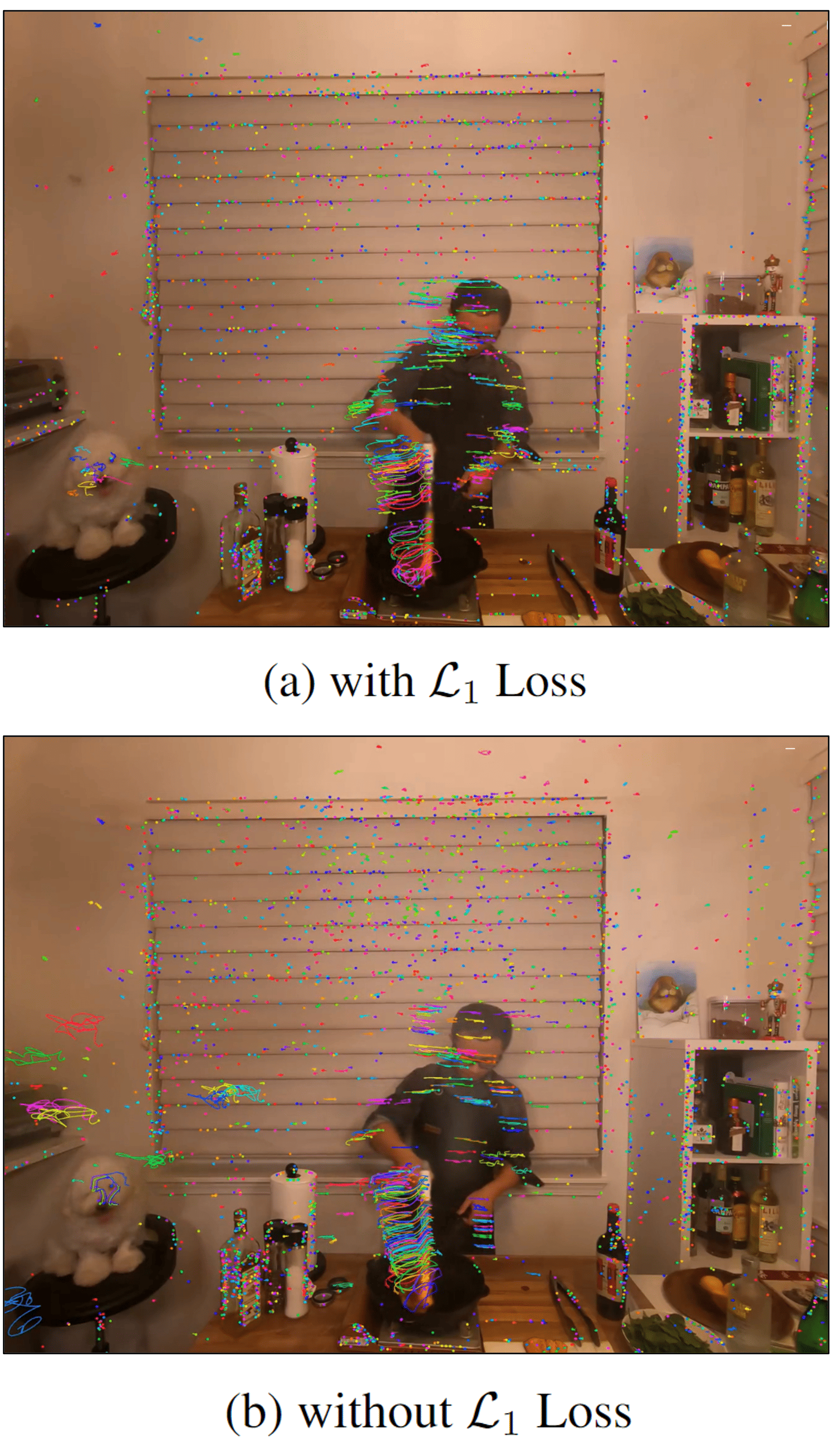
Figure 9: Qualitative comparison between using or not the $\mathcal{L}_{1}$ loss for regularizing the motion coefficients of each Gaussian. Results for the DyNeRF dataset.

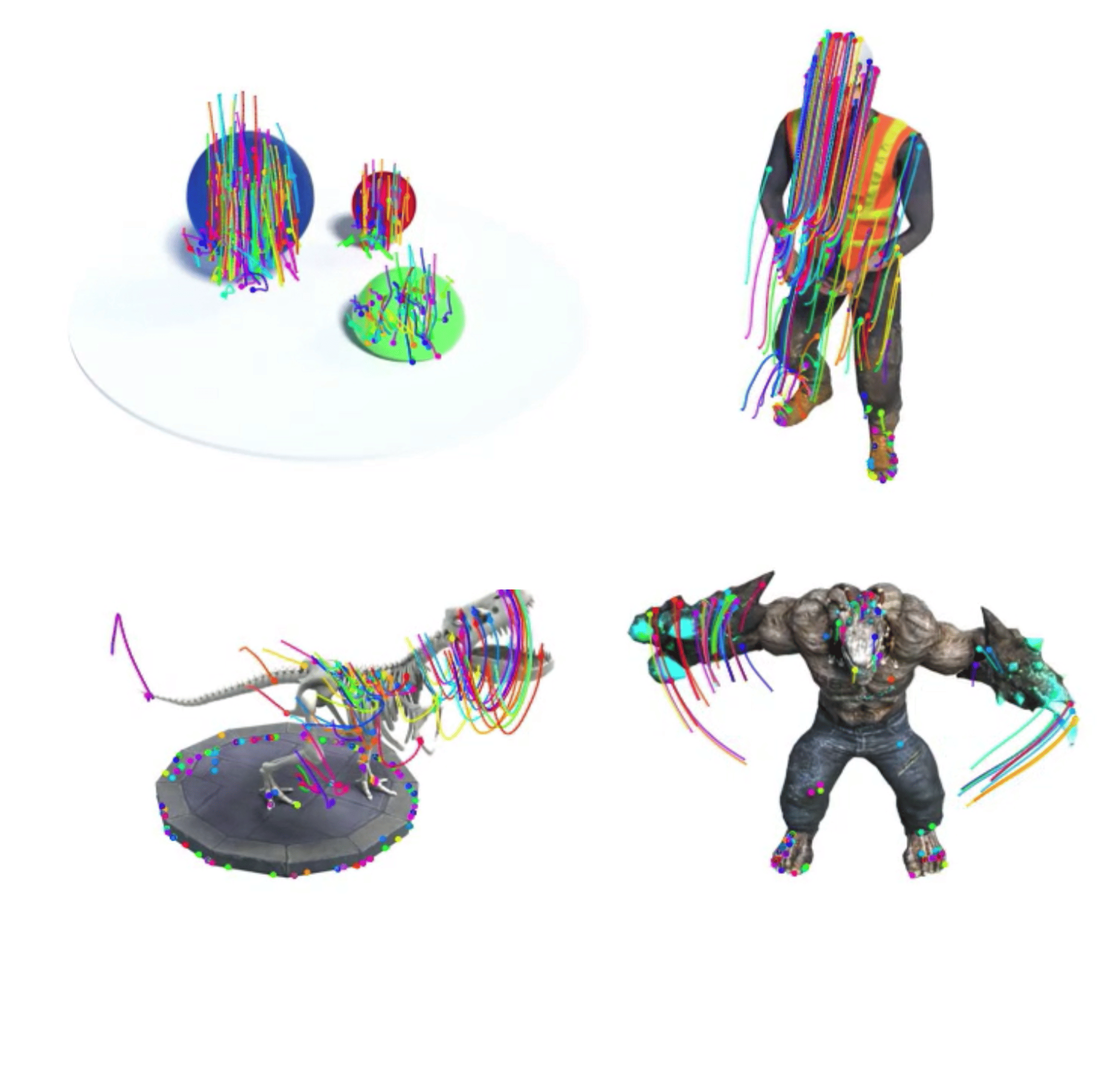
Figure 10: More visualizations on per-point trajectory tracking for the synthetic D-NeRF dataset.

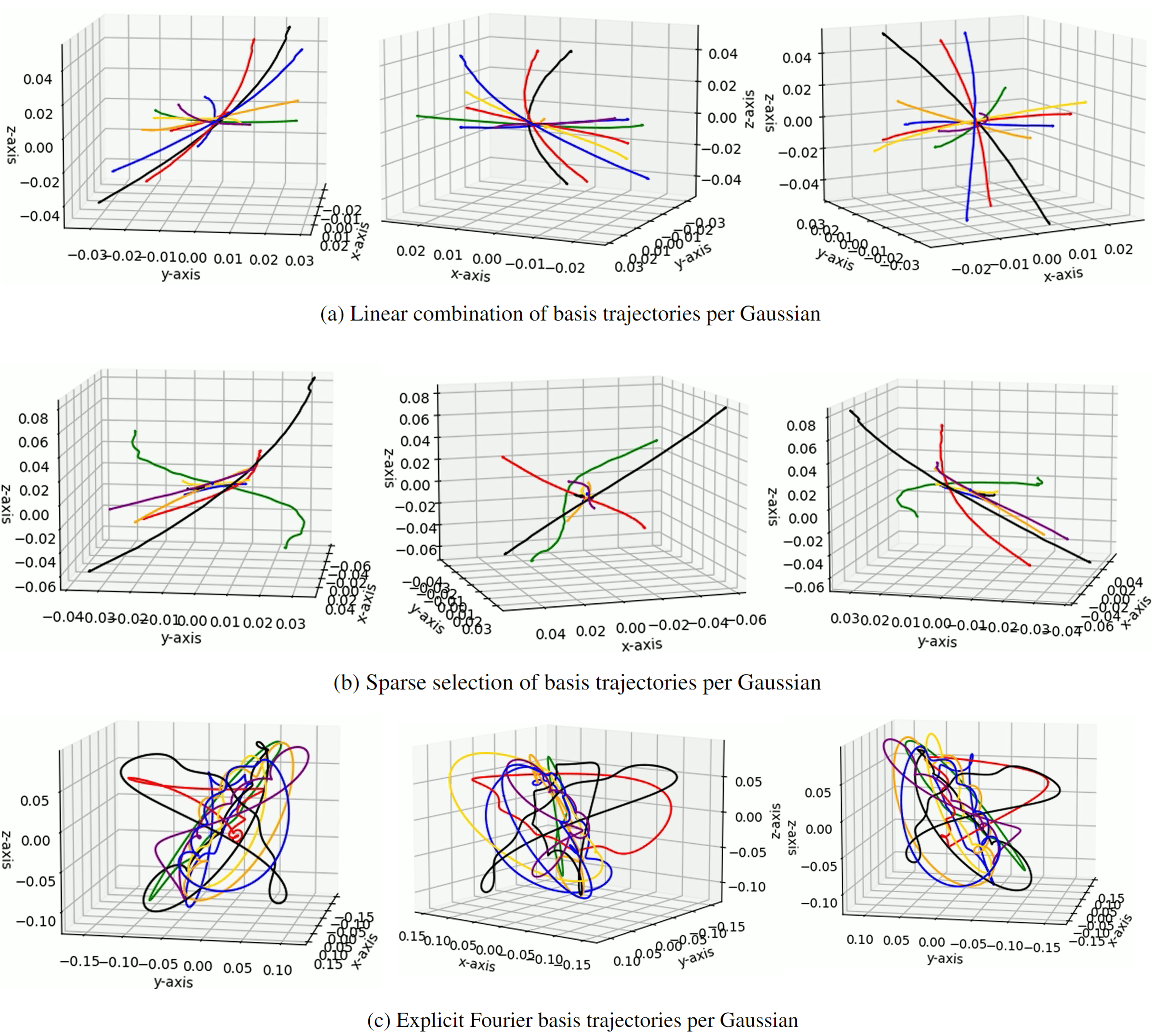
Figure 11: Visualization of the basis trajectories’ trace, along time, in the 3D world space. The results refer to the ’Mutant’ scene on the D-NeRF dataset. (a) The 10 basis trajectories without applying a sparsity loss and allowing each Gaussian to linearly combine all 10 of them to model its motion. (b) The 10 basis trajectories with the application of the sparsity loss, to enforce each Gaussian to choose only one trajectory for its motion. (c) The 10 basis trajectories explicitly modeled by the Fourier series instead of a smalled learned MLP.

Fourier basis: Instead of having a learned basis, we decided to experiment with an explicit basis as well; namely the Fourier series. We demonstrated that Fourier can somehow model the complex motions of a dynamic scene, which is expected from a global trajectory approximator. Nonetheless, it falls behind in terms of expressivity and rendering quality compared to a learned basis through a small MLP. Figure 11 depicts the learned or explicit trajectories that can model the dynamics of a scene. Specifically, each Gaussian can choose one or more of these 10 trajectories to model its unique motion in the dynamic scene. When we allow a linear combination of the 10 trajectories, then the basis functions are uniformly spread in the 3D world as depicted in Figure 11 (a). This is because each Gaussian can model its unique motion by linearly combining these motions, which lets it uniformly move in the space of the dynamic scene. If we restrict each Gaussian to choose only one trajectory, then these become more odd and specific to the motion needs of the corresponding scene, as in Figure 11 (b). Finally, in Figure 11 (c) we clearly see the periodic trace of the Fourier basis functions that are explicitly defined instead of learned by a small efficient MLP. We hypothesize that the complexity of the formed motion produced by the Fourier signals does not allow a sufficient convergence to an expressive enough solution. To model the roughly 3D linear trajectories produced by the MLP a much higher number of frequencies would be needed, making the optimization problem even more challenging.

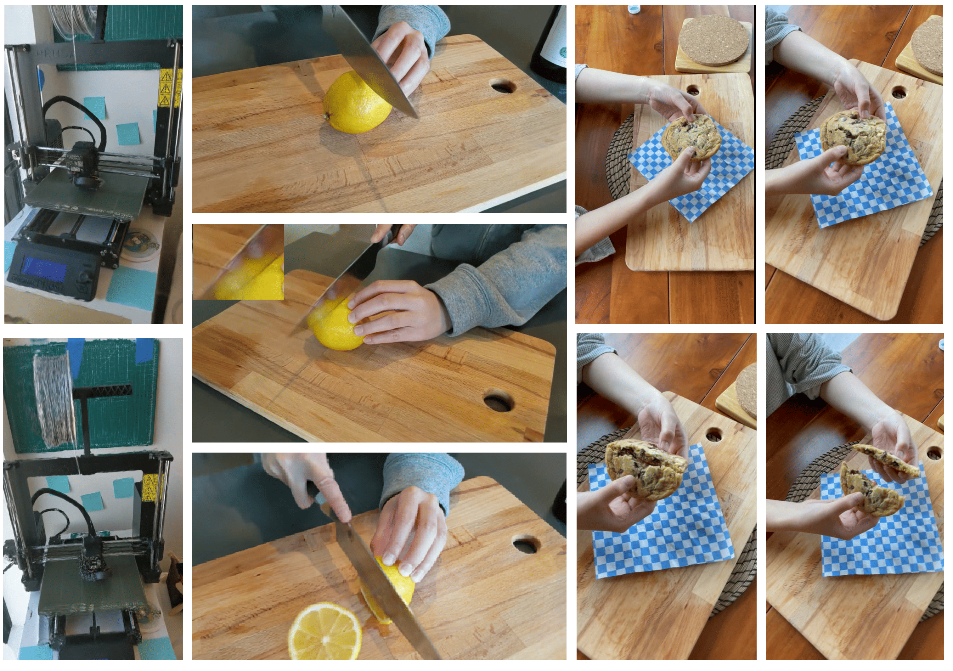
Figure 12: More qualitative rendering results on the HyperNeRF dataset from novel test views.

References

- Abou-Chakra et al. [2022] Jad Abou-Chakra, Feras Dayoub, and Niko Sünderhauf. Particlenerf: Particle based encoding for online neural radiance fields. arXiv preprint arXiv:2211.04041, 2022.
- Akhter et al. [2011] Ijaz Akhter, Yaser Sheikh, Sohaib Khan, and Takeo Kanade. Trajectory space: A dual representation for nonrigid structure from motion. IEEE Transactions on Pattern Analysis and Machine Intelligence, 33(7):1442–1456, 2011.
- Attal et al. [2023] Benjamin Attal, Jia-Bin Huang, Christian Richardt, Michael Zollhoefer, Johannes Kopf, Matthew O’Toole, and Changil Kim. HyperReel: High-fidelity 6-DoF video with ray-conditioned sampling. In Conference on Computer Vision and Pattern Recognition (CVPR), 2023.
- Barron et al. [2021] Jonathan T. Barron, Ben Mildenhall, Matthew Tancik, Peter Hedman, Ricardo Martin-Brualla, and Pratul P. Srinivasan. Mip-nerf: A multiscale representation for anti-aliasing neural radiance fields. ICCV, 2021.
- Barron et al. [2022] Jonathan T. Barron, Ben Mildenhall, Dor Verbin, Pratul P. Srinivasan, and Peter Hedman. Mip-nerf 360: Unbounded anti-aliased neural radiance fields. CVPR, 2022.
- Barron et al. [2023] Jonathan T. Barron, Ben Mildenhall, Dor Verbin, Pratul P. Srinivasan, and Peter Hedman. Zip-nerf: Anti-aliased grid-based neural radiance fields. ICCV, 2023.
- Cao and Johnson [2023] Ang Cao and Justin Johnson. Hexplane: A fast representation for dynamic scenes. CVPR, 2023.
- Chen et al. [2022] Anpei Chen, Zexiang Xu, Andreas Geiger, Jingyi Yu, and Hao Su. Tensorf: Tensorial radiance fields. In European Conference on Computer Vision (ECCV), 2022.
- Chen et al. [2023] Anpei Chen, Zexiang Xu, Xinyue Wei, Siyu Tang, Hao Su, and Andreas Geiger. Factor fields: A unified framework for neural fields and beyond. arXiv preprint arXiv:2302.01226, 2023.
- Collet et al. [2015] Alvaro Collet, Ming Chuang, Pat Sweeney, Don Gillett, Dennis Evseev, David Calabrese, Hugues Hoppe, Adam Kirk, and Steve Sullivan. High-quality streamable free-viewpoint video. ACM Trans. Graph., 34(4), 2015.
- Fang et al. [2022] Jiemin Fang, Taoran Yi, Xinggang Wang, Lingxi Xie, Xiaopeng Zhang, Wenyu Liu, Matthias Nießner, and Qi Tian. Fast dynamic radiance fields with time-aware neural voxels. In SIGGRAPH Asia 2022 Conference Papers, 2022.
- Fridovich-Keil et al. [2022] Sara Fridovich-Keil, Alex Yu, Matthew Tancik, Qinhong Chen, Benjamin Recht, and Angjoo Kanazawa. Plenoxels: Radiance fields without neural networks. In CVPR, 2022.
- Fridovich-Keil et al. [2023] Sara Fridovich-Keil, Giacomo Meanti, Frederik Rahbæk Warburg, Benjamin Recht, and Angjoo Kanazawa. K-planes: Explicit radiance fields in space, time, and appearance. In CVPR, 2023.
- Gan et al. [2022] Wanshui Gan, Hongbin Xu, Yi Huang, Shifeng Chen, and Naoto Yokoya. V4d: Voxel for 4d novel view synthesis, 2022.
- Kerbl et al. [2023] Bernhard Kerbl, Georgios Kopanas, Thomas Leimkühler, and George Drettakis. 3d gaussian splatting for real-time radiance field rendering. ACM Transactions on Graphics, 42(4), 2023.
- Kumar et al. [2017] Suryansh Kumar, Yuchao Dai, and Hongdong Li. Spatio-temporal union of subspaces for multi-body non-rigid structure-from-motion. Pattern Recognition, 71:428–443, 2017.
- Levoy and Hanrahan [1996] Marc Levoy and Pat Hanrahan. Light field rendering. ACM Transactions on Graphics (SIGGRAPH), 1996.
- Li et al. [2012] Hao Li, Linjie Luo, Daniel Vlasic, Pieter Peers, Jovan Popović, Mark Pauly, and Szymon Rusinkiewicz. Temporally coherent completion of dynamic shapes. ACM Trans. Graph., 31(1), 2012.
- Li et al. [2022] T. Li, M. Slavcheva, M. Zollhoefer, S. Green, C. Lassner, C. Kim, T. Schmidt, S. Lovegrove, M. Goesele, R. Newcombe, and Z. Lv. Neural 3d video synthesis from multi-view video. In 2022 IEEE/CVF Conference on Computer Vision and Pattern Recognition (CVPR), pages 5511–5521, Los Alamitos, CA, USA, 2022. IEEE Computer Society.
- Luiten et al. [2024] Jonathon Luiten, Georgios Kopanas, Bastian Leibe, and Deva Ramanan. Dynamic 3d gaussians: Tracking by persistent dynamic view synthesis. In 3DV, 2024.
- Mildenhall et al. [2020] Ben Mildenhall, Pratul P. Srinivasan, Matthew Tancik, Jonathan T. Barron, Ravi Ramamoorthi, and Ren Ng. Nerf: Representing scenes as neural radiance fields for view synthesis. In ECCV, 2020.
- Müller et al. [2022] Thomas Müller, Alex Evans, Christoph Schied, and Alexander Keller. Instant neural graphics primitives with a multiresolution hash encoding. ACM Trans. Graph., 41(4):102:1–102:15, 2022.
- Park et al. [2021a] Keunhong Park, Utkarsh Sinha, Jonathan T. Barron, Sofien Bouaziz, Dan B Goldman, Steven M. Seitz, and Ricardo Martin-Brualla. Nerfies: Deformable neural radiance fields. ICCV, 2021a.
- Park et al. [2021b] Keunhong Park, Utkarsh Sinha, Peter Hedman, Jonathan T. Barron, Sofien Bouaziz, Dan B Goldman, Ricardo Martin-Brualla, and Steven M. Seitz. Hypernerf: A higher-dimensional representation for topologically varying neural radiance fields. ACM Trans. Graph., 40(6), 2021b.
- Paszke et al. [2019] Adam Paszke, Sam Gross, Francisco Massa, Adam Lerer, James Bradbury, Gregory Chanan, Trevor Killeen, Zeming Lin, Natalia Gimelshein, Luca Antiga, Alban Desmaison, Andreas Kopf, Edward Yang, Zachary DeVito, Martin Raison, Alykhan Tejani, Sasank Chilamkurthy, Benoit Steiner, Lu Fang, Junjie Bai, and Soumith Chintala. Pytorch: An imperative style, high-performance deep learning library. In Advances in Neural Information Processing Systems 32, pages 8024–8035. Curran Associates, Inc., 2019.
- Pumarola et al. [2020] Albert Pumarola, Enric Corona, Gerard Pons-Moll, and Francesc Moreno-Noguer. D-NeRF: Neural Radiance Fields for Dynamic Scenes. In Proceedings of the IEEE/CVF Conference on Computer Vision and Pattern Recognition, 2020.
- Shao et al. [2023] Ruizhi Shao, Zerong Zheng, Hanzhang Tu, Boning Liu, Hongwen Zhang, and Yebin Liu. Tensor4d: Efficient neural 4d decomposition for high-fidelity dynamic reconstruction and rendering, 2023.
- Shenchang and Williams [1993] Eric Chen Shenchang and Lance Williams. View interpolation for image synthesis. ACM Transactions on Graphics (SIGGRAPH), 1993.
- Song et al. [2023] Liangchen Song, Anpei Chen, Zhong Li, Zhang Chen, Lele Chen, Junsong Yuan, Yi Xu, and Andreas Geiger. Nerfplayer: A streamable dynamic scene representation with decomposed neural radiance fields. IEEE Transactions on Visualization and Computer Graphics, 29(5):2732–2742, 2023.
- Sun et al. [2022] Cheng Sun, Min Sun, and Hwann-Tzong Chen. Direct voxel grid optimization: Super-fast convergence for radiance fields reconstruction. In CVPR, 2022.
- Tancik et al. [2020] Matthew Tancik, Pratul P. Srinivasan, Ben Mildenhall, Sara Fridovich-Keil, Nithin Raghavan, Utkarsh Singhal, Ravi Ramamoorthi, Jonathan T. Barron, and Ren Ng. Fourier features let networks learn high frequency functions in low dimensional domains. NeurIPS, 2020.
- Tancik et al. [2022] Matthew Tancik, Vincent Casser, Xinchen Yan, Sabeek Pradhan, Ben Mildenhall, Pratul Srinivasan, Jonathan T. Barron, and Henrik Kretzschmar. Block-NeRF: Scalable large scene neural view synthesis. arXiv, 2022.
- Valmadre and Lucey [2012] Jack Valmadre and Simon Lucey. General trajectory prior for non-rigid reconstruction. In 2012 IEEE Conference on Computer Vision and Pattern Recognition, pages 1394–1401, 2012.
- Wang et al. [2021a] Chaoyang Wang, Ben Eckart, Simon Lucey, and Orazio Gallo. Neural trajectory fields for dynamic novel view synthesis. In ArXiv Preprint, 2021a.
- Wang et al. [2022] Feng Wang, Sinan Tan, Xinghang Li, Zeyue Tian, and Huaping Liu. Mixed neural voxels for fast multi-view video synthesis. arXiv preprint arXiv:2212.00190, 2022.
- Wang et al. [2021b] Qianqian Wang, Zhicheng Wang, Kyle Genova, Pratul Srinivasan, Howard Zhou, Jonathan T. Barron, Ricardo Martin-Brualla, Noah Snavely, and Thomas Funkhouser. Ibrnet: Learning multi-view image-based rendering. In CVPR, 2021b.
- Wang et al. [2023] Qianqian Wang, Yen-Yu Chang, Ruojin Cai, Zhengqi Li, Bharath Hariharan, Aleksander Holynski, and Noah Snavely. Tracking everything everywhere all at once. In International Conference on Computer Vision, 2023.
- Wei et al. [2019] Mao Wei, Liu Miaomiao, Salzemann Mathieu, and Li Hongdong. Learning trajectory dependencies for human motion prediction. In ICCV, 2019.
- Weng et al. [2022] Chung-Yi Weng, Brian Curless, Pratul P. Srinivasan, Jonathan T. Barron, and Ira Kemelmacher-Shlizerman. HumanNeRF: Free-viewpoint rendering of moving people from monocular video. In Proceedings of the IEEE/CVF Conference on Computer Vision and Pattern Recognition (CVPR), pages 16210–16220, 2022.
- Wu et al. [2023] Guanjun Wu, Taoran Yi, Jiemin Fang, Lingxi Xie, Xiaopeng Zhang, Wei Wei, Wenyu Liu, Qi Tian, and Wang Xinggang. 4d gaussian splatting for real-time dynamic scene rendering. arXiv preprint arXiv:2310.08528, 2023.
- Yang et al. [2022] Gengshan Yang, Minh Vo, Natalia Neverova, Deva Ramanan, Andrea Vedaldi, and Hanbyul Joo. Banmo: Building animatable 3d neural models from many casual videos. In CVPR, 2022.
- Yang et al. [2023a] Ziyi Yang, Xinyu Gao, Wen Zhou, Shaohui Jiao, Yuqing Zhang, and Xiaogang Jin. Deformable 3d gaussians for high-fidelity monocular dynamic scene reconstruction. arXiv preprint arXiv:2309.13101, 2023a.
- Yang et al. [2023b] Zeyu Yang, Hongye Yang, Zijie Pan, Xiatian Zhu, and Li Zhang. Real-time photorealistic dynamic scene representation and rendering with 4d gaussian splatting. arXiv preprint arXiv 2310.10642, 2023b.
- Zhang et al. [2020] Kai Zhang, Gernot Riegler, Noah Snavely, and Vladlen Koltun. Nerf++: Analyzing and improving neural radiance fields. arXiv:2010.07492, 2020.
- Zhang et al. [2022] Qiang Zhang, Seung-Hwan Baek, Szymon Rusinkiewicz, and Felix Heide. Differentiable point-based radiance fields for efficient view synthesis. In SIGGRAPH Asia 2022 Conference Papers, New York, NY, USA, 2022. Association for Computing Machinery.
- Zhang et al. [2021] Yan Zhang, Michael J Black, and Siyu Tang. We are more than our joints: Predicting how 3d bodies move. In Proceedings of the IEEE/CVF Conference on Computer Vision and Pattern Recognition, pages 3372–3382, 2021.
- Zhao et al. [2022] Fuqiang Zhao, Wei Yang, Jiakai Zhang, Pei Lin, Yingliang Zhang, Jingyi Yu, and Lan Xu. Humannerf: Efficiently generated human radiance field from sparse inputs. In Proceedings of the IEEE/CVF Conference on Computer Vision and Pattern Recognition (CVPR), pages 7743–7753, 2022.
- Zhu and Lucey [2015] Yingying Zhu and Simon Lucey. Convolutional sparse coding for trajectory reconstruction. IEEE Transactions on Pattern Analysis and Machine Intelligence, 37(3):529–540, 2015.
- Zwicker et al. [2002] Matthias Zwicker, Hanspeter Pfister, Jeroen Van Baar, and Markus Gross. Ewa splatting. IEEE Transactions on Visualization and Computer Graphics, 8(3):223–238, 2002.