CLIP-QDA: An Explainable Concept Bottleneck Model

Abstract

In this paper, we introduce an explainable algorithm designed from a multi-modal foundation model, that performs fast and explainable image classification. Drawing inspiration from CLIP-based Concept Bottleneck Models (CBMs), our method creates a latent space where each neuron is linked to a specific word. Observing that this latent space can be modeled with simple distributions, we use a Mixture of Gaussians (MoG) formalism to enhance the interpretability of this latent space. Then, we introduce CLIP-QDA, a classifier that only uses statistical values to infer labels from the concepts. In addition, this formalism allows for both local and global explanations. These explanations come from the inner design of our architecture, our work is part of a new family of greybox models, combining performances of opaque foundation models and the interpretability of transparent models. Our empirical findings show that in instances where the MoG assumption holds, CLIP-QDA achieves similar accuracy with state-of-the-art methods CBMs. Our explanations compete with existing XAI methods while being faster to compute.

1 Introduction

The field of artificial intelligence is advancing rapidly, driven by sophisticated models like Deep Neural Networks (LeCun et al., 2015) (DNNs). These models find extensive applications in various real-world scenarios, including conversational chatbots (Ouyang et al., 2022), neural machine translation (Liu et al., 2020), and image generation (Rombach et al., 2021). Although these systems demonstrate remarkable accuracy, the process behind their decision-making often remains obscure. Consequently, deep learning encounters certain limitations and drawbacks. The most notable one is the lack of transparency regarding their behavior, which leaves users with limited insight into how specific decisions are reached. This lack of transparency becomes particularly problematic in high-stakes situations, such as medical diagnoses or autonomous vehicles.

The imperative to scrutinize the behavior of DNNs has become increasingly compelling as the field gravitates towards methods of larger scale in terms of both data utilization and number of parameters involved, culminating in what is commonly referred to as “foundation models” (Brown et al., 2020; Radford et al., 2021; Ramesh et al., 2021). These models have demonstrated remarkable performance, particularly in the domain of generalization, while concurrently growing more intricate and opaque. Additionally, there is a burgeoning trend in the adoption of multimodality (Reed et al., 2022), wherein various modalities such as sound, image, and text are employed to depict a single concept. This strategic use of diverse data representations empowers neural networks to transcend their reliance on a solitary data format. Nonetheless, the underlying phenomena that govern the amalgamation of these disparate inputs into coherent representations remain shrouded in ambiguity and require further investigation.

The exploration of latent representations is crucial for understanding the internal dynamics of a DNN. DNNs possess the capability to transform input data into a space, called latent space, where inputs representing the same semantic concept are nearby. For example, in the latent space of a DNN trained to classify images, two different images of cats would be mapped to points that are close to each other (Johnson et al., 2016). This capability is further reinforced through the utilization of multimodality (Akkus et al., 2023), granting access to neurons that represent abstract concepts inherent to multiple types of data signals.

A class of networks that effectively exploits this notion is Concept Bottleneck Models (CBMs) (Koh et al., 2020). CBMs are characterized by their deliberate construction of representations for high-level human-understandable concepts, frequently denoted as words. Remarkably, there is a growing trend in employing CLIP (Radford et al., 2021), a foundation model that establishes a shared embedding space for both text and images, to generate concept bottleneck models in an unsupervised manner.

Unfortunately, while CLIP embeddings represent tangible concepts, the derived values, often termed “CLIP scores” pose challenges in terms of interpretation. Furthermore, to the best of our knowledge, there is a notable absence of studies that seek to formally characterize CLIP’s latent space. The underlying objective here is to gain insights into how the pre-trained CLIP model organizes a given input distribution. Consequently, there is an opportunity to develop mathematically rigorous methodologies for elucidating the behavior of CLIP.

Then, our contributions are summarized as follows:

• We propose to represent the distribution of CLIP scores by a mixture of Gaussians. This representation enables a mathematically interpretable classification of images using human-understandable concepts.

• Utilizing the modeling approach presented in this study, we use Quadratic Discriminant Analysis (QDA) to classify the labels from the concepts, we name this method CLIP-QDA. CLIP-QDA demonstrates competitive performance when compared to existing CBMs based on CLIP. Notably, CLIP-QDA achieves this level of performance while utilizing a reduced set of parameters, limited solely to statistical values, including means, covariance matrices, and label probabilities.

• We propose two efficient and mathematically grounded XAI metrics for model explanation. These metrics encompass both global and local assessments of why the model behaves. The global metric directly emanates from our Gaussian modeling approach, providing a comprehensive evaluation of CLIP-QDA’s performance. Additionally, our local metric draws inspiration from counterfactual analysis, furnishing insights into individual data points.

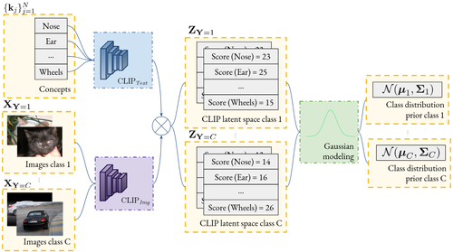
Figure 1: Overview of our modeling method. By considering the whole dataset CLIP scores ${\bm{z}}$ as class conditioned distributions ${\bm{Z}}=\begin{bmatrix}Z^{{\color[rgb]{0,0,0}1}}&\ldots&Z^{{\color[rgb]{0,0,0}N}}\end{bmatrix}$, we model the CLIP latent space as a mixture of Gaussians, allowing for mathematically grounded explanations.

2 Background and Related Work

2.1 Contrastive Image Language Pre-training (CLIP)

CLIP (Radford et al., 2021) is a state-of-the-art model that can jointly process image and text inputs. The model was pre-trained on a large dataset of images and texts to learn to associate visual and textual concepts. Then, the capacity of CLIP to create a semantically rich encoding induced the creation of many emergent models in detection, few-shot learning, or image captioning.

The widespread adoption of CLIP stems from the remarkable robustness exhibited by its pre-trained model. Through training on an extensive multimodal dataset, such as Schuhmann et al. (2022), the model achieves impressive performance. Thus, on few- and zero-shot learning, for which it was designed, it obtains impressive results across a wide range of datasets. Notably, CLIP provides a straightforward and efficient means of obtaining semantically rich representations of images in low-dimensional spaces. This capability enables researchers and practitioners to divert the original use of CLIP to various other applications (Luo et al., 2022; Menon & Vondrick, 2022).

While the concept of CBM has its origins prior to the rise of DNNs (Kumar et al., 2009; Lampert et al., 2009), and CLIP (Koh et al., 2020; Losch et al., 2019), the emergence of this multimodal foundational model has opened up novel opportunities. Recent research (Yang et al., 2023; Oikarinen et al., 2023) has leveraged large language models to directly construct concepts from CLIP text embeddings, opening the door to a family of CLIP-based CBMs. Additionally, efforts have been made to create sparse CLIP-based CBMs (Panousis et al., 2023; Feng et al., 2023). Yan et al. (2023a) explore methods to achieve superior representations with minimal labels. Yuksekgonul et al. (2022) capitalize on the CLIP embedding spaces, considering concepts as activation vectors. Finally, Kim et al. (2023) build upon the idea of activation vectors to discover counterfactuals.

2.2 Explainable AI

According to Arrieta et al. (2020), we can define an explainable model as a computational model, that is designed to provide specific details or reasons to ensure clarity and ease of understanding regarding its functioning. In broader terms, an explanation denotes the information or output that an explainable model delivers to elucidate its operational processes.

The literature shows a clear distinction between non-transparent (or blackbox) and transparent (or whitebox) models. Transparent models are characterized by their inherent explainability. These models can be readily explained due to their simplicity and easily interpretable features. Examples of such models include linear regression (Galton, 1886), logistic regression (McCullagh, 2019), and decision trees (Quinlan, 1986). In contrast, non-transparent models are inherently non-explainable. This category encompasses models that could have been explainable if they possessed simpler and more interpretable features (Galton, 1886; Quinlan, 1986), as well as models that inherently lack explainability, including deep neural networks. The distinction between these two types of models highlights the trade-off between model complexity and interpretability (Arrieta et al., 2020), with transparent models offering inherent explainability while non-transparent models allow for better performance, but require the use of additional techniques for explanations, named post-hoc methods. Commonly used post-hoc methods include visualization techniques, such as saliency maps (Selvaraju et al., 2017), which highlight the influential features in an image that contribute to the model’s decision-making. Sensitivity analysis (Cortez & Embrechts, 2011) represents another avenue, involving the analysis of model predictions by varying input data. Local explanation techniques are also used to explain the model from a local simplification of the model around a point of interest (Ribeiro et al., 2016; Plumb et al., 2018). Finally, feature relevance techniques aim at estimating the impact of each feature on the decision (Lundberg & Lee, 2017).

In an endeavor to integrate the strengths of both black and whitebox models, the concept of greybox XAI has been introduced by Bennetot et al. (2022). These models divide the overall architecture into two distinct components. Initially, a blackbox model is employed to process high-entropy input signals, such as images, and transform them into a lower-entropy latent space that is semantically meaningful and understandable by humans. By leveraging the blackbox model’s ability to simplify complex problems, a whitebox model is then used to deduce the final result based on the output of the blackbox model. This approach yields a partially explainable model that outperforms traditional whitebox models while retaining partial transparency, in a unified framework.

3 Method

3.1 General framework

For our experimental investigations, we consider a general framework based on prior work on CLIP-based CBMs (Yang et al., 2023; Oikarinen et al., 2023). This framework consists of two core components. The first component centers on the extraction of multi-modal features, enabling the creation of connections between images and text. The second component encompasses a classifier head. A visual depiction of this process is presented in Figure 2.

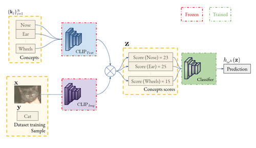
Figure 2: Training procedure of the general framework. First, CLIP scores ${\bm{z}}$ are computed for each of the concepts $\{{\bm{k}}^{j}\}_{j=1}^{N}$, then a classifier $h_{{\bm{\omega}}^{h}}(.)$, with parameters ${\bm{\omega}}^{h}$ is trained to classify the label from the concatenation of the CLIP scores.

We build upon CLIP DNN (Radford et al., 2021), which enables the creation of a multi-modal latent space through the fusion of image and text information. Rather than relying on a single text or prompt, we employ a set of diverse prompts, each representing distinct concepts. These concepts remain consistent across the dataset and are not subject to alterations. The purpose of CLIP’s representation is to gauge the similarities between each concept and an image, thereby giving rise to a latent space. To prevent ambiguity, we denote the resulting space of CLIP scores as the “CLIP latent space”, while the spaces generated by the text and image encoders are respectively referred to as the “CLIP text embedding space” and the “CLIP image embedding space”. Here, “CLIP score” denotes the value derived from a cosine distance computation between the image and text encodings.

The selection of concepts is guided by expert input and acts as a hyperparameter within our framework. For comprehensive examples of concept sets, please refer to Section A.1. It is noteworthy that there is no requirement for individual image annotation with these concepts. This is due to CLIP’s inherent design, which allows it to score concepts in a zero-shot manner.

Following the acquisition of the CLIP latent space, it is given as an input to a classifier head, which is responsible for learning to predict the class. Thanks to the low dimension of the latent space and the clear semantics of each component (concepts), it is possible to design simple and explainable classifiers.

3.2 CLIP latent space analysis

3.2.1 Notations and formalism

Let us introduce the following notations used in the rest of the paper. $X$ and $Y$ represent two random variables (RVs) with joint distribution $(X,Y)\sim\mathcal{P}_{X,Y}$. A realization of this distribution is a pair $({\bm{x}},y)$ that concretely represents one image and its label. In particular, $y$ takes values in $\llbracket 1,C\rrbracket$, with $C\in\mathbb{N}$ the number of classes. From this distribution, we can deduce the marginal distributions $X\sim\mathcal{P}_{X}$ and $Y\sim\mathcal{P}_{Y}$. We can also describe for each class $c$, an RV $X_{Y=c}\sim\mathcal{P}_{X_{Y=c}}$ that represents the conditional distribution of images that have the class $c$.

Let $\{{\bm{k}}^{j}\}_{j=1}^{N}$ denote a set of $N\in\mathbb{N}$ concepts, where each ${\bm{k}}^{j}$ is a character string representing the concept in natural language. We consider “CLIP’s DNN” to refer to the vector of its pre-trained weights, denoted as ${\bm{\omega}}^{g}$, and a function $g$ that represents the architecture of the deep neural network (DNN). Given an image ${\bm{x}}$ and a concept ${\bm{k}}^{j}$, the output of CLIP’s DNN is represented as $z^{j}=g_{{\bm{\omega}}^{g}}({\bm{x}},{\bm{k}}^{j})$. The projection in the multi-modal latent space of an image ${\bm{x}}$ is the vector ${\bm{z}}=\begin{bmatrix}g_{{\bm{\omega}}^{g}}({\bm{x}},{\bm{k}}^{{\color[rgb]{0,0,0}1}})&\ldots&g_{{\bm{\omega}}^{g}}({\bm{x}},{\bm{k}}^{{\color[rgb]{0,0,0}N}})\end{bmatrix}$. We define $Z^{j}$ as the random variable associated with the observation $z^{j}$. It should be noted that ${\bm{Z}}=\begin{bmatrix}Z^{{\color[rgb]{0,0,0}1}}&\ldots&Z^{{\color[rgb]{0,0,0}N}}\end{bmatrix}$ is the random variable representing the concatenation of the CLIP scores associated with the $N$ concepts. Furthermore, we denote the conditional distributions of ${\bm{z}}$ having class $c$ as ${\bm{Z}}_{Y=c}=\begin{bmatrix}Z^{{\color[rgb]{0,0,0}1}}_{Y=c}&\ldots&Z^{{\color[rgb]{0,0,0}N}}_{Y=c}\end{bmatrix}$.

Finally, we define the classifier as a function $h_{{\bm{\omega}}^{h}}({\bm{z}})$ with parameters ${\bm{\omega}}^{h}$ that, given a vector ${\bm{z}}$, attributes the predicted class.

3.2.2 Gaussian modeling of CLIP’s latent space

To analyze the behavior of the CLIP latent space, we conduct a thorough examination of the distribution of CLIP scores. To elucidate our modeling approach, we suggest to visualize a large set of samples from $Z^{j}$ by observing the CLIP scores of an entire set of images taken from a toy example, which consists of images representing only cats and cars (see the Cats/Cars dataset in Section 4.1). In this instance, the concept denoted by “$j$” corresponds to “Pointy-eared”.

In Figure 3, which illustrates the histogram of CLIP scores, we observe that the distribution exhibits characteristics that can be effectively modeled as a mixture of two Gaussians. The underlying intuition here is that the distribution $Z^{j}$ represents two types of images: those without pointy ears, resulting in the left mode (low scores) of CLIP scores, and those with pointy ears, resulting in the right mode (high scores). Since this concept uniquely characterizes the classes – cats have ears but not cars – we can assign each mode to a specific class. This intuition is corroborated by the visualization of the distribution $Z^{j}_{Y=1}$ (Car) in violet and the distribution $Z^{j}_{Y=2}$ (Cat) in red. Since the extracted distributions exhibit similarities to normal distributions, we are motivated to describe ${\bm{Z}}$ as a mixture of Gaussians. Yet, we also discuss the validity and limitations of this modeling approach in Section 4.2.

(a) Modeling of $p_{c}Z_{Y=c}$.

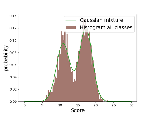
(b) Modeling of $Z$.

Figure 3: Normalized histogram of scores $Z^{j}$ specifically for the concept “Pointy-eared”. On the left, we observe that the different classes can be modeled as weighted Gaussians. On the right, we show the resulting Gaussian mixture modeling.

Mathematically, the Gaussian prior assumption is equivalent to:

$$p({\bm{Z}}={\bm{z}}\mid Y=c)=\mathcal{N}({\bm{z}}\mid{\bm{\mu}}_{c},{\bm{\Sigma}}_{c}),\$$ (1)

where ${\bm{\Sigma}}_{c}$ and ${\bm{\mu}}_{c}$ are the mean vectors and the covariance matrices, different for each class. Moreover, given the multinomial distribution of $Y$, with the notation $p_{c}=P(Y=c)$, we can model ${\bm{Z}}$ as a mixture of Gaussians:

$$p({\bm{Z}}={\bm{z}})= \sum_{c=1}^{C}p_{c}\mathcal{N}({\bm{z}}\mid{\bm{\mu}}_{c},{\bm{\Sigma}}_{c})\ .$$ (2)

3.3 CLIP Quadratic Discriminant Analysis

Based on the Gaussian distribution assumption described in Section 3.2.2, a natural choice for $h_{{\bm{\omega}}^{h}}$ (the classifier in Figure 2) is the Quadratic Discriminant Analysis (QDA) as defined in Hastie et al. (2009). To compute it, we need to estimate the parameters $({\bm{\Sigma}}_{c},{\bm{\mu}}_{c},p_{c})$ of the probability distributions ${\bm{Z}}_{Y=c}$ and $Y$, which is done by computing the maximum likelihood estimators on the training data.

Subsequently, with the knowledge of the functions $p({\bm{Z}}={\bm{z}}\mid Y=c)$ and $p(Y=c)$, we can apply Bayes theorem to make an inference on $p(Y=c\mid{\bm{Z}}={\bm{z}})$:

$$p(Y=c\mid{\bm{Z}}={\bm{z}})=\frac{p_{c}\mathcal{N}({\bm{z}}\mid{\bm{\mu}}_{c},{\bm{\Sigma}}_{c})}{\sum_{c=1}^{N}p_{c}\mathcal{N}({\bm{z}}\mid{\bm{\mu}}_{c},{\bm{\Sigma}}_{c})}\,.$$ (3)

Then, the output of the QDA classifier can be described as:

$$h_{{\bm{\omega}}^{h}}({\bm{z}})=\underset{c}{\arg\max}~{}~{}\frac{p_{c}}{(2\pi)^{N/2}|{\bm{\Sigma}}_{c}|^{1/2}}e^{-\frac{1}{2}({\bm{z}}-{\bm{\mu}}_{c})^{T}{\bm{\Sigma}}_{c}^{-1}({\bm{z}}-{\bm{\mu}}_{c})}\,.$$ (4)

In practice, we leverage the training data to estimate ${\bm{\omega}}^{h}=({\bm{\Sigma}}_{c},{\bm{\mu}}_{c},p_{c})$, which enables us to bypass the standard stochastic gradient descent process, resulting in an immediate “training time”. Furthermore, this classifier offers the advantage of transparency, akin to the approach outlined by Arrieta et al. (2020), with its parameters comprising identifiable statistical values and its output values representing probabilities.

3.4 XAI Metrics

Since our description of the CLIP latent space is grounded in a probabilistic framework, we have access to a range of statistical tools for interpreting the way our classifier works. In this section, we introduce two distinct types of explanations: a global explanation that provides insights into the way the classifier acts on the entire dataset (see Section 3.4.1), and a local explanation designed to elucidate the model’s behavior on a specific sample (see Section 3.4.2).

3.4.1 Global metric

As we have access to priors that describe the distribution of each class, a valuable insight to gain an understanding of which concept our classifier aligns with is the measurement of distances between these distributions. Specifically, we focus on the conditional distributions of two classes of interest $c_{1}$ and $c_{2}$, that we denote by $Z^{j}_{Y=c_{1}}$ and $Z^{j}_{Y=c_{2}}$. The underlying intuition behind measuring the distance between these distributions is that the larger the distance, the more the attribute $j$ can differentiate between the classes $c_{1}$ and $c_{2}$.

To accomplish this, we propose to use the Wasserstein-2 distance as a metric for quantifying the separation between the two conditional distributions. It is worth noting that calculating the Wasserstein-2 distance can be a complex task in general. However, for Gaussian distributions, there exists a closed-form solution for computing the Wasserstein-2 distance. In addition, we sign the distance to keep the information of the position of $c_{1}$ relative to $c_{2}$:

$$\tilde{W_{2}}(Z^{j}_{Y=c_{1}},Z^{j}_{Y=c_{2}}) =\text{sign}([{\bm{\mu}}_{c_{1}}]_{(j)}-[{\bm{\mu}}_{c_{2}}]_{(j)})\left(([{\bm{\mu}}_{c_{1}}]_{(j)}-[{\bm{\mu}}_{c_{2}}]_{(j)})^{2}+\Lambda^{j}_{c_{1},c_{2}}\right),$$

where $\Lambda^{j}_{c_{1},c_{2}}=[{\bm{\Sigma}}_{c_{1}}]_{(j,j)}+[{\bm{\Sigma}}_{c_{2}}]_{(j,j)}-2{\color[rgb]{0,0,0}\sqrt{[{\bm{\Sigma}}_{c_{1}}]_{(j,j)}[{\bm{\Sigma}}_{c_{2}}]_{(j,j)}}}$.

Note that the resulting value is no longer a distance since we lost the commutativity property. Examples of explanations based on this metric are given in Sections 4.4 and A.4.

3.4.2 Local metric

One would like to identify the key concepts associated with a particular image that plays a pivotal role in achieving the task’s objective. To delve deeper into the importance and relevance of concepts in the decision-making process of the classifier, a widely accepted approach is to generate counterfactuals (Plumb et al., 2022; Luo et al., 2023; Kim et al., 2023). If a small perturbation of a concept score changes the class, the concept is considered important. We now formalize this mathematically.

Consider a pre-trained classifier denoted as $h_{{\bm{\omega}}^{h}}(\cdot)$. In this context, ${\bm{\omega}}^{h}$ represents the set of weights associated with the CLIP-QDA, specifically ${\bm{\omega}}^{h}=({\bm{\Sigma}}_{c},{\bm{\mu}}_{c},p_{c})$. Given a score vector ${\bm{z}}$, we define counterfactuals as hypothetical values ${\bm{z}}+{\bm{\epsilon}}^{j}_{{\color[rgb]{0,0,0}s}}$, ${\bm{\epsilon}}^{j}_{{\color[rgb]{0,0,0}s}}$ being called the perturbation. This perturbation aims to be of minimal magnitude and is obtained by solving the following optimization problem:

$$\min\|{\bm{\epsilon}}^{j}_{{\color[rgb]{0,0,0}s}}\|^{2}~{}~{}\textnormal{s.t.}~{}~{}h_{{\bm{\omega}}^{h}}({\bm{z}}+\epsilon^{j}_{s})\neq h_{{\bm{\omega}}^{h}}({\bm{z}})\,.$$ (5)

The idea behind this equation is to find the minimal perturbation ${\bm{\epsilon}}^{j}_{{\color[rgb]{0,0,0}s}}$ of the input ${\bm{z}}$ that makes the classifier produce a different label than $h_{{\bm{\omega}}^{h}}({\bm{z}})$. However, in our case, two important restrictions are applied to ${\bm{\epsilon}}^{j}_{{\color[rgb]{0,0,0}s}}$:

1. Sparsity: for interpretability, we only change one attribute at a time, indicated by the index $j$. Then ${\bm{\epsilon}}^{j}_{{\color[rgb]{0,0,0}s}}=[0,..,0,\epsilon^{j}_{{\color[rgb]{0,0,0}s}},0,...,0]$.

2. Sign: we take into account the sign $s\in\{-,+\}$ of the perturbation. Then, we separate the positive counterfactuals ${\bm{\epsilon}}^{j}_{{\color[rgb]{0,0,0}+}}=[0,..,0,\epsilon^{j}_{+},0,...,0],~{}\epsilon^{j}_{+}\in\mathbb{R^{+}}$ and the negative counterfactuals. ${\bm{\epsilon}}^{j}_{-}=[0,..,0,\epsilon^{j}_{-},0,...,0],~{}\epsilon^{j}_{-}\in\mathbb{R^{-}}$.

These two constraints are imposed to generate concise and, consequently, more informative counterfactuals. In this context, if a solution to equation 5, denoted as ${\bm{\epsilon}}^{j}_{s,*}$, exists, it represents the minimal modification (addition or subtraction) to the coordinate $j$ of the original vector ${\bm{z}}$ that results in a change from $h_{{\bm{\omega}}^{h}}({\bm{z}})$ to $h_{{\bm{\omega}}^{h}}({\bm{z}}+{\bm{\epsilon}}^{j}_{s,*})$. Note that this approach allows for an explicit evaluation of the effect of an intervention, denoted as $do({\bm{Z}}={\bm{z}}+\epsilon^{j}_{s})$ using a common notation in causal inference (Peters et al., 2017). Concretely, this emulates answers to questions of the form: “Would the label of my cat’s image change if I removed a certain amount of its pointy ears?”.

Another important point to notice is that to obtain all possible counterfactuals, this equation must be solved for all concepts $j$ and both signs $s$. A practical way to compute counterfactuals is given below.

Proposition 1.

Let us consider a pre-trained QDA classifier $h_{{\bm{\omega}}^{h}}(.)$ with parameters ${\bm{\omega}}^{h}$. Assume that the input data is drawn from the corresponding Gaussian Mixture model, as defined in 4, and that ${\bm{\epsilon}}^{j}_{s}$ a perturbation with the above sparsity and sign restrictions. Then, there is a closed-form solution to problem 5, which is a function of the parameters $({\bm{\Sigma}}_{c},{\bm{\mu}}_{c},p_{c})_{c=1}^{C}$.

The proof and expression are given in Appendix A.2. We illustrate the behavior of our classifier and our local metric with a toy example which consists of two Gaussians ($C=2$) among two concepts $Z_{1}$ and $Z_{2}$ ($N=2$). We find the counterfactuals for both signs following the first concept (${\bm{\epsilon}}^{{\color[rgb]{0,0,0}1}}_{-,*}$ and ${\bm{\epsilon}}^{{\color[rgb]{0,0,0}1}}_{+,*}$). Results are presented in Figure 4.

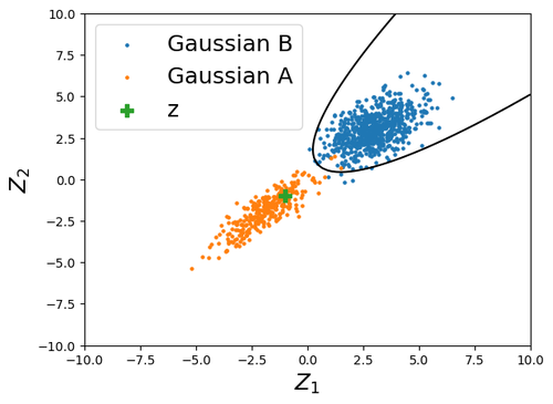
(a) In this case, the input sample (in green) does not have counterfactuals by only changing $z_{1}$.

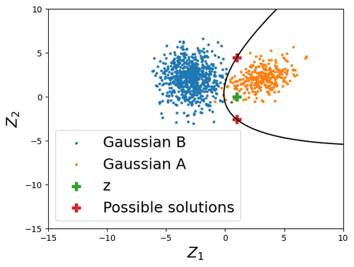
(b) In this case, the input sample (in green) has counterfactuals ${\bm{\epsilon}}^{1}_{-,*}$ and ${\bm{\epsilon}}^{1}_{+,*}$. Changing $z_{1}$ leads to two intersections with the equiprobability line, one by adding score, the other by removing score.

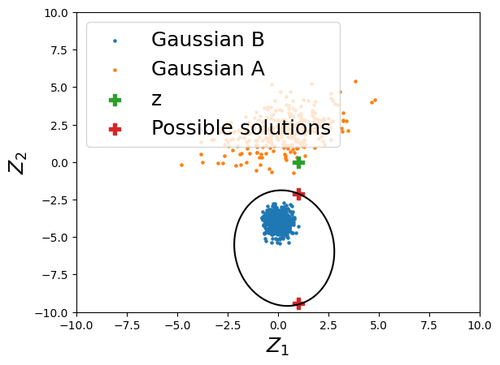
(c) In this case, the input sample (in green) only has one counterfactual ${\bm{\epsilon}}^{1}_{-,*}$ and no counterfactual ${\bm{\epsilon}}^{1}_{+,*}$. Changing $z_{1}$ leads to two intersections with the equiprobability line, but since both are by removing score, only the one of minimal magnitude is conserved.

Figure 4: Visualization of the counterfactuals in the two Gaussians toy example. Samples of the two distributions are plotted in blue and orange. The equiprobability line is plotted in black.

It is worth noting that these counterfactual values are initially expressed in CLIP score units, which may not inherently provide meaningful interpretability. To mitigate this limitation, we introduce scaled counterfactuals, denoted as ${\bm{\epsilon}}^{j}_{s,*,scaled}$, obtained by dividing each counterfactual by the standard deviation associated with its respective distribution:

$${\bm{\epsilon}}^{j}_{s,*,scaled}=\frac{{\bm{\epsilon}}^{j}_{s,*}}{\sqrt{[{\bm{\Sigma}}_{c}]_{(j,j)}}}\,.$$ (6)

Then, the value of each counterfactual can be expressed as “the addition (or subtraction) of standard deviations in accordance to ${\bm{Z}}_{Y=h_{{\bm{\omega}}^{h}}({\bm{z}})}$ that changes the label”. Examples of such explanations are given in Sections 4.4 and A.4.

4 Experiments

4.1 Experimental setup

We evaluate our methods on ImageNet (Deng et al., 2009), PASCAL-Part (Donadello & Serafini, 2016), MIT Indoor Scenes dataset (Quattoni & Torralba, 2009), Monumai (Lamas et al., 2021) and Flowers102 (Nilsback & Zisserman, 2008). In addition to these well-established datasets, we introduce a custom dataset named Cats/Dogs/Cars dataset. To construct this dataset, we concatenated three widely recognized datasets, namely, the Kaggle Cats and Dogs Dataset (Cukierski, 2013) and the Standford Cars Dataset (Krause et al., 2013). Subsequently, we filtered the dataset to exclusively contain images of white and black animals and cars. This curation resulted in six distinct subsets: “Black Cars”, “Black Dogs”, “Black Cats”, “White Cars”, “White Dogs”, “White Cats”. The primary objective of this dataset is to facilitate experiments under conditions of substantial data bias, such as classifying white cats when the training data has only encountered white dogs and black cats. In its final form, the dataset comprises 6,436 images.

In addition to CLIP-QDA, we also test our method with linear regression as a classifier from CLIP scores, frequently named linear probe classifier. The objective here is to provide a comparison with existing CLIP-CBMs (Yang et al., 2023; Yan et al., 2023a; b).

4.2 Gaussian prior hypothesis

In this section, we investigate to which extent the Gaussian prior hypothesis (Equation 1) holds. To assess this, we use Chi-Square Q-Q plots (Chambers, 2018; Mahalanobis, 2018), a normality assessment method adapted to multidimensional data. We display Chi-Square Q-Q plots on the conditional distribution $({{\bm{Z}}\mid Y=c})$, with data sourced from PASCAL-Part and class $c$ = “aeroplane”. First, we compute a set of concepts adapted to the output class, following the procedure described in Appendix A.1. Subsequently, we perform the same experiment with a set of words specifically dedicated to the class of interest (Figure 5(a)). In addition, we show a visualization with randomly chosen concepts from the PASCAL-Part set of concepts, as depicted in Figure 5(b).

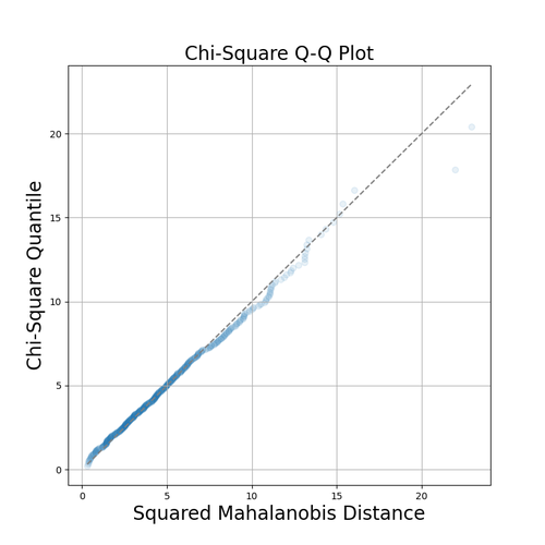
(a) CBM with a set of concepts related to the label “Aeroplane”: [Winged, Jet engines, Tail fin, Fuselage, Landing gear]

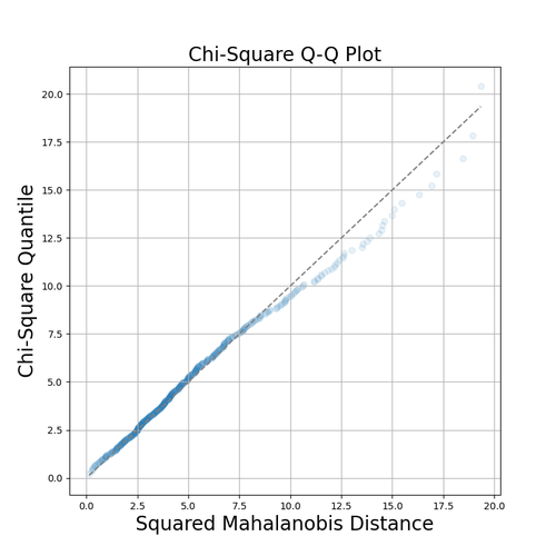
(b) CBM with a set of concepts unrelated to the label “Aeroplane”: [Furry, Equine, Container or pot, Saddle or seat, Multi-doored]

Figure 5: Multivariate QQplot for a Gaussian fit for the PASCAL-Part images that have the label “Aeroplane”.

Notably employing a less precise set of concepts can introduce disturbances, as evidenced in the observations. As indicated in Section 3.2.2, the ambiguity associated with certain concepts, such as “Multi-doored”, can lead to bimodal distributions (an aeroplane having one, multiple, or no doors). In Figure 6, we shows the histogram of the clip scores ${\bm{z}}$ of the images that have the class “aeroplane”. Compared to the histogram of less ambiguous cases (like in 3), we observe that the histogram presents anomalies, especially around the mean.

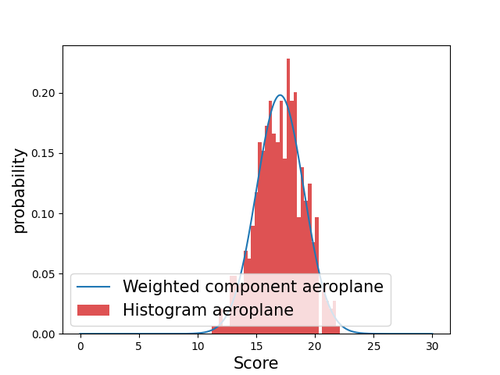
Figure 6: Histogram and Gaussian fitting of CLIP scores ${\bm{z}}$ for images that have the class “aeroplane” of the attribute “Multi-doored”.

Additionally, we performed a similar experiment with larger sets of concepts. We selected random subsets containing 10, 15, and 20 concepts from the PASCAL-Part set listed in Table 2. The outcomes are displayed in Figure 7. In this scenario, it becomes obvious that the Gaussian assumption is increasingly violated as the number of concepts grows. Indeed, as the number of concepts increases, the likelihood of encountering ambiguous concepts in each sample significantly rises, which undermines the feasibility of modeling the data as an unimodal Gaussian distribution.

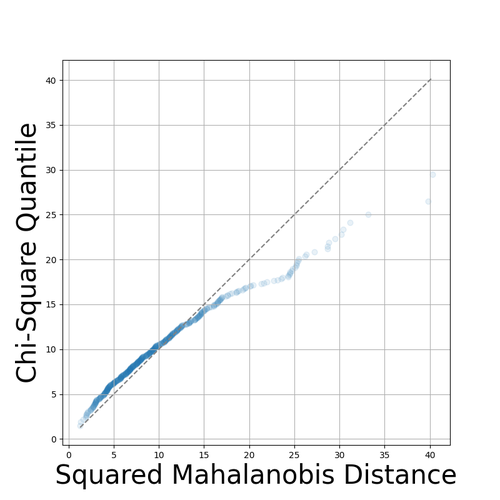
(a) CBM with 10 concepts

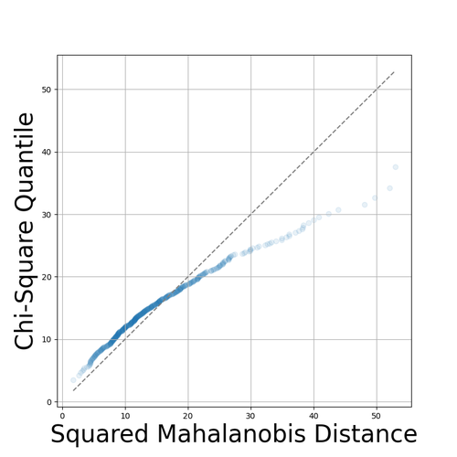
(b) CBM with 15 concepts

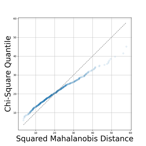
(c) CBM with 20 concepts

Figure 7: Multivariate QQplot for a Gaussian fit for the PASCAL-Part images that have the label “Aeroplane”.

4.3 Classification accuracy

Comparison with other classifiers.

In this section, we undertake a comparative evaluation of the performance of our CLIP-QDA classifier in contrast to other classifiers commonly employed in contemporary research. Precisely, we compare our method to the use of CLIP as a zero-shot classifier, by making predictions based on the class that produces the maximum CLIP score with the image embedding. We also use the linear probe, which consists of using a linear layer as the classifier of the CBM (see Figure 2). Our assessment is based on the computation of accuracy metrics across three diverse datasets: PASCAL-Part, MIT scenes, and Monumai. A comprehensive description of the procedure for concept set acquisition is provided in Appendix A.1. Furthermore, for contextualization, we include in the table the test accuracy of ResNet (He et al., 2016) and ViT (Dosovitskiy et al., 2021) trained in a supervised manner by using images as inputs.

Table 1: Test set accuracy.

Method	PASCAL-Part	MIT scenes	Monumai
CLIP (zero shot)	0,81	0,63	0,52
CLIP + linear probe	0,91	0,77	0,81
CLIP + QDA probe	0,90	0,81	0,89
Resnet 50 (He et al., 2016)	0,84	0,86	0,95
ViT-L 336px (Dosovitskiy et al., 2021)	0,95	0,94	0,94

Our findings reveal that fine-tuning using CBM, either as a linear or a QDA probe, significantly improves performance, as evidenced by the increase in accuracy compared to using CLIP as a zero-shot classifier. This improvement is particularly pronounced on datasets dedicated to specialized tasks, such as Monumai. Additionally, CLIP CBMs tend to achieve performances comparable to networks trained from raw images, making these models appealing for image classification due to their reduced training cost in both time and resources, as well as their interpretability. Notably, CLIP-QDA demonstrates competitive performance, when compared to linear probe techniques. However, a slight decrease in performance is observed, especially in the PASCAL-Part dataset. This decline could be attributed to the use of a larger set of concepts specifically for this dataset, posing challenges to the Gaussian assumption and potentially affecting the applicability of our classifier.

Influence of the number of concepts.

To assess the influence of the number of concepts $C$ on the accuracy, we conduct experiments on the PASCAL-Part dataset. These experiments involve testing accuracy for both QDA and linear probe with concept sets of different lengths, all generated following the methodology described in Section A.1. As seen in Figure 8, CLIP-QDA performs better than linear probe when the number of concepts is relatively low. In contrast, the linear probe outperforms CLIP-QDA as the number of concepts increases. This observation aligns with the insights gained from the discussion on Gaussian modeling in Section 4.2, where a higher number of concepts challenges the grounding assumptions of CLIP-QDA.

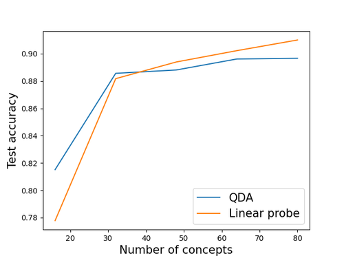
Figure 8: Accuracy of the classifiers for different concept sizes. QDA refers to the use of CLIP-QDA. Linear probe refers to the use of a linear layer as a classifier.

4.4 XAI metrics

4.4.1 Global metric

To evaluate the relevance of our explanations, we present a toy example from our Cats/Dogs/Cars dataset by constructing a CBM consisting of the concepts Table 2, plus the concepts “Black” and “White”. Next, we display the 10 most influential concepts according to our global metric (the top 10 concepts that have the highest Wasserstein distance).

We present the results in Figure 9 for two scenarios: one with an unbiased dataset containing cats and cars of both colors and the other one with only black cats and white cars. We can observe that in the biased dataset, the concepts “Black” and “White” hold significantly higher importance, indicating that the classifier is likely to be biased about these concepts. This shows that our global explanation method has a potential for detecting biases in datasets (Tommasi et al., 2017). Additional explanation samples for various use cases are available in Appendix A.4.

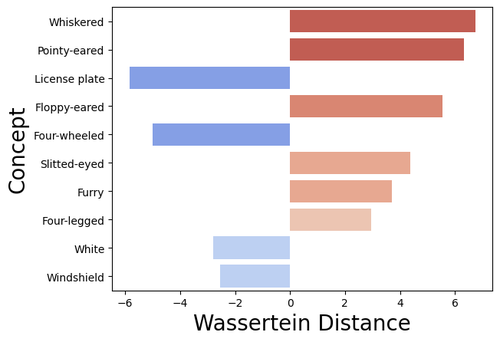
(a) Unbiased dataset

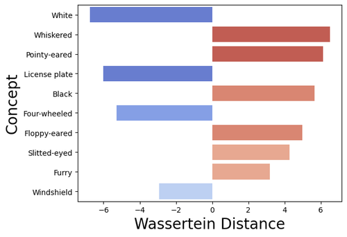
(b) Biased dataset

Figure 9: Global explanation on subsets of Cats/Cars. Here, $c_{1}$=“Cat” and $c_{2}$=“Car”. Positive values indicate concepts that are more prevalent in cat images than car images, while negative values indicate concepts that are more common in car images compared to cat images. We display here only the top 10 concepts that have the highest Wasserstein distance (the concept “Black” is positioned $15^{th}$ in the unbiased setup).

4.4.2 Local metrics

Test on a biased dataset.

In this section, we show an application of our local metric within the framework of our biased dataset, as previously described. We keep the same setup, employing a training set consisting of white cats and black cars. Subsequently, we feed an image of a white cat into our classifier (Figure 10). It is noteworthy that the image is misclassified as a car. Our local metric demonstrates sensitivity to the dataset’s color bias, corroborating the warning issued by the global explanation.

(a) Input image

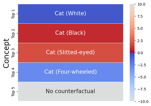
(b) Top 5 concepts. Classifier inference=“Car”

Figure 10: Local explanation on subsets of Cats/Cars. On the right figure, the blue/red scale represents the scaled counterfactuals as in equation 6, the text in each box corresponds to the label predicted after the perturbation, followed to the concept changed to obtained its result (in parentheses). According to the explanation, we can note that removing a little of the concept “White”, or adding a little of the concept “Black” to the vector ${\bm{z}}$ induces a change of label to the correct one, thus highlighting the bias of the dataset.

Comparison to post-hoc methods.

We compare our local explanation method with popular post-hoc methods, namely LIME (Ribeiro et al., 2016) and SHAP (Lundberg & Lee, 2017). This involves treating CLIP scores as tabular data to generate explanations for the classifier’s decisions. These post-hoc methods can be more time-consuming, as illustrated in Figure A.3. This increased computational cost arises from their approach of analyzing the model’s behavior based on the output response to various perturbed inputs, rather than directly examining the model’s parameters.

To conduct this evaluation, we designed an experiment based on the deletion metric (Petsiuk et al., 2018). The procedure involves taking each sample from the test set and nullifying (i.e., setting to the average value of the score across classes) a certain number, $N_{null}$, of concepts. We nullify the concepts based on their importance order as determined by each explanation method. If nullifying the concepts leads to a significant decrease in performance, we consider it a successful selection of concepts that influenced the classifier’s decision. Our experiment is conducted using the unbiased version of the Cats/Dogs/Cars dataset. It is organized into two setups: the first one uses the concept set from Table 2, and the second one uses an equal number of concepts randomly selected from a dictionary of words. The results are presented in Figure 11.

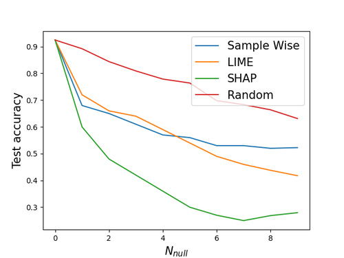
(a) Random set of concepts

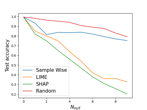
(b) Set of concepts that tailored to the dataset

Figure 11: Deletion test accuracies. The lower the accuracy is, the more faithful the explanation method is. Random refers to the use of a random selection of concepts to nullify.

In the random words setup, our local metric demonstrates competitive performance compared to LIME but lags behind SHAP. However, in the adapted word set scenario, we observed significantly worse results. This might be explained by the high correlation among the resulting CLIP scores from this word set, leading to situations akin to Figure 4(a), where searching for counterfactuals attribute by attribute struggled to provide meaningful insights. Globally, the classification boundaries obtained from our QDA are relevant for areas that present a high density of training samples, which is not the case for many of the counterfactuals.

5 Conclusion

In this paper, we introduce a modeling approach for the embedding space of CLIP, a foundation model trained on a vast dataset. Our observations reveal that CLIP can organize information in a distribution that exhibits similarities with a mixture of Gaussians. Building upon this insight, we develop an adapted concept bottleneck model that demonstrates competitive performance along with transparency. While the model that we have presented offers the advantage of simplicity and a limited number of parameters, it does encounter challenges when dealing with a broader and more ambiguous set of concepts. As a suggestion for future research, we propose to extend this modeling approach to incorporate other priors, such as Laplacian distributions, and to explore more complex models, including those with multiple components, i.e., using more than one Gaussian to describe a class for example. Additionally, our research is centered around a specific embedding space (CLIP scores). Exploring similar work on other latent spaces, particularly those associated with multimodal foundation models, could be valuable to determine if similar patterns exist in those spaces.

Appendix A Appendix

A.1 Set of concepts

Inspired by Yang et al. (2023), we use large language models to provide concept sets. Concretely, we use GPT-3 (Brown et al., 2020) with the following preprompt: “In this task, you have to give visual descriptions that describe an image. Respond as a list. Each item being a word.” Then, we generate the sets of words by the following prompt: “What are [N] useful visual descriptors to distinguish a [class] in a photo?” By doing so, we generated 5 concepts per class, presented in Table 2.

Table 2: List of concepts used.

Dataset	Set of concepts
PASCAL-Part	’aeroplane’:[’Winged, Jet engines, Tail fin, Fuselage, Landing gear’],’bicycle’:[’Two-wheeled, Pedals, Handlebars, Frame, Chain-driven’],’bird’:[’Feathery, Beaked, Wingspread, Perched, Avian’],’bottle’:[’Glass or plastic, Cylindrical, Necked, Cap or cork, Transparent or translucent’],’bus’:[’Large, Rectangular, Windows, Wheels, Multi-doored’],’cat’:[’Furry, Whiskered, Pointy-eared, Slitted-eyed, Four-legged’],’car’:[’Metallic, Four-wheeled, Headlights, Windshield, License plate’],’dog’:[’Snout, Wagging-tailed, Snout-nosed, Floppy-eared, Tail-wagging’],’cow’:[’Bovine, Hooved, Horned (in some cases), Spotted or solid-colored, Grazing (if in a field)’],’horse’:[’Equine, Hooved, Maned, Tailed, Galloping (if in motion)’],’motorbike’:[’Two-wheeled , Engine, Handlebars , Exhaust, Saddle or seat’],’person’:[’Human, Facial features, Limbs (arms and legs), Clothing, Posture or stance’],’pottedplant’:[’Potted, Green, Leaves, Soil or potting mix, Container or pot’],’sheep’:[’Woolly, Hooved, Grazing, Herded (if in a group), White or colored fleece’],’train’:[’Locomotive, Railcars, Tracks, Wheels , Carriages’],’tvmonitor’:[’Screen, Rectangular , Frame or bezel, Stand or wall-mounted, Displaying an image’]
Monumai	’Baroque’:[’Ornate, Elaborate sculptures, Intricate details, Curved or asymmetrical design, Historical or aged appearance’],’Gothic’:[’Pointed arches, Ribbed vaults, Flying buttresses, Stained glass windows, Tall spires or towers’],’Hispanic muslim’:[’Mudejar style, Intricate geometric patterns, Horseshoe arches, Decorative tilework (azulejos), Islamic-inspired motifs’],’Rennaissance’:[’Classical proportions, Symmetrical design, Columns and pilasters, Human statues and sculptures, Dome or dome-like structures’]
MIT scenes	’Store’:[’Building or structure, Signage or banners, Glass windows or doors, Displayed products or merchandise, People entering or exiting (if applicable)’],’Home’:[’Residential, Roofed, Windows, Landscaping or yard, Front entrance or door’],’Public space’:[’Open area, Crowds (if people are present), Benches or seating, Pathways or walkways, Architectural features (e.g., buildings, statues)’],’Leisure’:[’Recreational, Play equipment (if applicable), Greenery or landscaping, Picnic tables or seating, Relaxing atmosphere’],’Working space’:[’Office equipment (e.g., desks, computers), Task-oriented, Office chairs, Organized or structured, People working (if applicable)’]
Cats/Dogs/Cars	’Cat’:[’Furry, Whiskered, Pointy-eared, Slitted-eyed, Four-legged’],’Car’:[’Metallic, Four-wheeled, Headlights, Windshield, License plate’],’Dog’:[’Snout, Wagging-tailed, Snout-nosed, Floppy-eared, Tail-wagging’]

A.2 Closed-form solution of counterfactuals for CLIP QDA

First, we will derive the resolution of equation 5 for the binary case before extending it to the multiclass case. Let us begin with a binary classifier, where ${Y\in\{h_{{\bm{\omega}}^{h}}({\bm{z}}),\overline{h_{{\bm{\omega}}^{h}}({\bm{z}})}\}}$ (for convenience, we note $h_{{\bm{\omega}}^{h}}({\bm{z}})=c_{h}$ and $\overline{h_{{\bm{\omega}}^{h}}({\bm{z}})}=c_{\overline{h}}$ ).

Proposition 2.

Let $h_{{\bm{\omega}}^{h}}$ a binary classifier and ${\bm{Z}}$ following a mixture of Gaussians such as ${\bm{Z}}_{Y=c_{h}}\sim\mathcal{N}({\bm{\mu}}_{{c_{h}}},\,{\bm{\Sigma}}_{{{{c_{h}}}}})$ and ${\bm{Z}}_{Y=c_{\overline{h}}}\sim\mathcal{N}({\bm{\mu}}_{{c_{\overline{h}}}},\,{\bm{\Sigma}}_{c_{\overline{h}}}^{-1})$ and ${\bm{\epsilon}}^{j}_{s}$ a perturbation with the above sparsity and sign restrictions. Then, there is a closed form solution to problem 5, given by:

$$\epsilon_{s}^{j}=\begin{cases}\emptyset~{}~{}\textnormal{if}~{}~{}b^{2}-4Pc<0~{}\\ \textnormal{or}~{}(s\neq\textnormal{sign}(b_{1})~{}\textnormal{and}~{}s\neq\textnormal{sign}(b_{2}))\\ \\ b_{1}~{}~{}\textnormal{if}~{}~{}b^{2}-4Pc>0~{}~{}\textnormal{and}~{}~{}\textnormal{sign}(b_{1})=s\\ \textnormal{and}~{}~{}(\textnormal{sign}(b_{2})\neq s~{}~{}\textnormal{or}~{}~{}|b_{2}|\geq|b_{1}|)\\ \\ b_{2}~{}~{}\textnormal{if}~{}~{}b^{2}-4Pc>0~{}~{}\textnormal{and}~{}~{}\textnormal{sign}(b_{2})=s\\ \textnormal{and}~{}~{}(\textnormal{sign}(b_{1})\neq s~{}~{}\textnormal{or}~{}~{}|b_{1}|>|b_{2}|),\end{cases}$$ (7)

with:

$$P=\frac{1}{2}\left([{\bm{\Sigma}}_{c_{\overline{h}}}^{-1}]_{(j,j)}-[{\bm{\Sigma}}_{c_{h}}^{-1}]_{(j,j)}\right)$$

$$b=\sum_{k=1}^{N}\left(([{\bm{z}}]_{(k)}-[{\bm{\mu}}_{{c_{\overline{h}}}}]_{(k)})[{\bm{\Sigma}}_{c_{\overline{h}}}^{-1}]_{(j,k)}-([{\bm{z}}]_{(k)}-[{\bm{\mu}}_{{c_{h}}}]_{(k)})[{\bm{\Sigma}}_{c_{h}}^{-1}]_{(j,k)}\right)$$

$$c=\frac{1}{2}\log\left[\frac{|{\bm{\Sigma}}_{c_{\overline{h}}}|}{|{\bm{\Sigma}}_{c_{h}}|}\right]+\log\left[\frac{p_{c_{h}}}{p_{c_{\overline{h}}}}\right]+\frac{1}{2}({\bm{z}}-{\bm{\mu}}_{c_{\overline{h}}})^{\top}{\bm{\Sigma}}_{c_{\overline{h}}}^{-1}({\bm{z}}-{\bm{\mu}}_{c_{\overline{h}}})-\frac{1}{2}({\bm{z}}-{\bm{\mu}}_{c_{h}})^{\top}{{{\bm{\Sigma}}_{c_{h}}^{-1}}}({\bm{z}}-{\bm{\mu}}_{c_{h}})$$

$$b_{1}=\frac{-b-\sqrt{b^{2}-4Pc}}{2P}$$ (8)

$$b_{2}=\frac{-b+\sqrt{b^{2}-4Pc}}{2P}\,.$$

Proof.

For the binary case, equation 5 can be written as :

$$\min\|{\bm{\epsilon}}^{j}_{{\color[rgb]{0,0,0}s}}\|^{2}~{}~{}\textnormal{s.t.}\quad\frac{p_{c_{\overline{h}}}}{(2\pi)^{N/2}|{\bm{\Sigma}}_{c_{\overline{h}}}|^{\frac{1}{2}}}e^{-\frac{1}{2}({\bm{z}}+{\bm{\epsilon}}^{j}_{{\color[rgb]{0,0,0}s}}-{\bm{\mu}}_{c_{\overline{h}}})^{T}{\bm{\Sigma}}_{c_{\overline{h}}}^{-1}({\bm{z}}+{\bm{\epsilon}}^{j}_{{\color[rgb]{0,0,0}s}}-{\bm{\mu}}_{c_{\overline{h}}})}\leqslant\frac{p_{c_{h}}}{(2\pi)^{N/2}|{\bm{\Sigma}}_{c_{h}}|^{\frac{1}{2}}}e^{-\frac{1}{2}({\bm{z}}+{\bm{\epsilon}}^{j}_{{\color[rgb]{0,0,0}s}}-{\bm{\mu}}_{{c_{h}}})^{T}{\bm{\Sigma}}_{c_{h}}^{-1}({\bm{z}}+{\bm{\epsilon}}^{j}_{{\color[rgb]{0,0,0}s}}-{\bm{\mu}}_{{c_{h}}})}.$$ (9)

Let us focus on the inequality constraint:

$$\hfill\frac{p_{c_{\overline{h}}}}{|{\bm{\Sigma}}_{c_{\overline{h}}}|^{\frac{1}{2}}}~{}~{}e^{-\frac{1}{2}({\bm{z}}+{\bm{\epsilon}}^{j}_{s}-{\bm{\mu}}_{{c_{\overline{h}}}})^{T}{\bm{\Sigma}}_{c_{\overline{h}}}^{-1}({\bm{z}}+{\bm{\epsilon}}^{j}_{s}-{\bm{\mu}}_{{c_{\overline{h}}}})}\leqslant~{}~{}\frac{p_{c_{h}}}{|{\bm{\Sigma}}_{c_{h}}|^{\frac{1}{2}}}~{}~{}e^{-\frac{1}{2}({\bm{z}}+{\bm{\epsilon}}^{j}_{s}-{\bm{\mu}}_{{c_{h}}})^{T}{\bm{\Sigma}}_{c_{h}}^{-1}({\bm{z}}+{\bm{\epsilon}}^{j}_{s}-{\bm{\mu}}_{{c_{h}}})}\hfill\\ \iff\log(p_{c_{\overline{h}}})-\frac{1}{2}\log|{\bm{\Sigma}}_{c_{\overline{h}}}|-\frac{1}{2}({\bm{z}}+{\bm{\epsilon}}^{j}_{s}-{\bm{\mu}}_{c_{\overline{h}}})^{T}{\bm{\Sigma}}_{c_{\overline{h}}}^{-1}({\bm{z}}+{\bm{\epsilon}}^{j}_{s}-{\bm{\mu}}_{c_{\overline{h}}})\hfill\\ \hfill\leqslant~{}~{}\log(p_{c_{h}})-\frac{1}{2}\log|{\bm{\Sigma}}_{c_{h}}|-\frac{1}{2}({\bm{z}}+{\bm{\epsilon}}^{j}_{s}-{\bm{\mu}}_{{c_{h}}})^{T}{\bm{\Sigma}}_{c_{h}}^{-1}({\bm{z}}+{\bm{\epsilon}}^{j}_{s}-{\bm{\mu}}_{{c_{h}}})\\ \iff\log(p_{c_{\overline{h}}})-\frac{1}{2}\log|{\bm{\Sigma}}_{c_{\overline{h}}}|-\frac{1}{2}({\bm{z}}-{\bm{\mu}}_{{c_{\overline{h}}}})^{T}{\bm{\Sigma}}_{c_{\overline{h}}}^{-1}({\bm{z}}-{\bm{\mu}}_{{c_{\overline{h}}}})-\frac{1}{2}{{\bm{\epsilon}}^{j}_{s}}^{T}{\bm{\Sigma}}_{c_{\overline{h}}}^{-1}{\bm{\epsilon}}^{j}_{s}-{{\bm{\epsilon}}^{j}_{s}}^{T}{\bm{\Sigma}}_{c_{\overline{h}}}^{-1}({\bm{z}}-{\bm{\mu}}_{{c_{\overline{h}}}})\hfill\\ \hfill\leqslant~{}~{}\log(p_{c_{h}})-\frac{1}{2}\log|{\bm{\Sigma}}_{c_{h}}|-\frac{1}{2}({\bm{z}}-{\bm{\mu}}_{{c_{h}}})^{T}{\bm{\Sigma}}_{c_{h}}^{-1}({\bm{z}}-{\bm{\mu}}_{{c_{h}}})-\frac{1}{2}{{\bm{\epsilon}}^{j}_{s}}^{T}{\bm{\Sigma}}_{c_{h}}^{-1}{\bm{\epsilon}}^{j}_{s}-{{\bm{\epsilon}}^{j}_{s}}^{T}{\bm{\Sigma}}_{c_{h}}^{-1}({\bm{z}}-{\bm{\mu}}_{{c_{h}}})\\ \iff\log(p_{c_{\overline{h}}})-\frac{1}{2}\log|{\bm{\Sigma}}_{c_{\overline{h}}}|-\frac{1}{2}({\bm{z}}-{\bm{\mu}}_{{c_{\overline{h}}}})^{T}{\bm{\Sigma}}_{c_{\overline{h}}}^{-1}({\bm{z}}-{\bm{\mu}}_{{c_{\overline{h}}}})-\frac{1}{2}[{\bm{\Sigma}}_{c_{\overline{h}}}^{-1}]_{(j,j)}(\epsilon^{j}_{s})^{2}-\epsilon^{j}_{s}\sum_{k=1}^{N}([{\bm{z}}]_{(k)}-[{\bm{\mu}}_{{c_{\overline{h}}}}]_{(k)})[{\bm{\Sigma}}_{c_{\overline{h}}}^{-1}]_{(j,k)}\hfill\\ \hfill\leqslant~{}~{}\log(p_{c_{h}})-\frac{1}{2}\log|{\bm{\Sigma}}_{c_{h}}|-\frac{1}{2}({\bm{z}}-{\bm{\mu}}_{{c_{h}}})^{T}{\bm{\Sigma}}_{c_{h}}^{-1}({\bm{z}}-{\bm{\mu}}_{{c_{h}}})-\frac{1}{2}[{\bm{\Sigma}}_{c_{h}}^{-1}]_{(j,j)}(\epsilon^{j}_{s})^{2}-\epsilon^{j}_{s}\sum_{k=1}^{N}([{\bm{z}}]_{(k)}-[{\bm{\mu}}_{{c_{h}}}]_{(k)})[{\bm{\Sigma}}_{c_{h}}^{-1}]_{(j,k)}\\ \iff\hfill P(\epsilon^{j}_{s})^{2}+b\epsilon^{j}_{s}+c\geqslant 0\,.\hfill$$

Then we can rewrite the problem as :

$$\min~{}({\bm{\epsilon}}^{j}_{s})^{2}~{}~{}\textnormal{s.t.}~{}~{}P(\epsilon^{j}_{s})^{2}+b\epsilon^{j}_{s}+c \leqslant 0.$$ (10)

To solve this problem, we introduce slack variables $\lambda$ and $I$, and define a Lagrangian as:

$$L({\bm{\epsilon}}^{j}_{s},\lambda,I)=(\epsilon^{j}_{s})^{2}+\lambda(P(\epsilon^{j}_{s})^{2}+b\epsilon^{j}_{s}+c+I^{2})\,.$$ (11)

Then, we can find the possible solutions by solving the system :

$$\begin{cases}\frac{\partial L}{\partial\epsilon^{j}_{s}}=0\\ \frac{\partial L}{\partial\lambda}=0\\ \frac{\partial L}{\partial I}=0,\end{cases}$$

which corresponds to:

$$\begin{cases}2(\lambda P+1)\epsilon^{j}_{s}+\lambda b=0\\ P(\epsilon^{j}_{s})^{2}+b\epsilon^{j}_{s}+c+I^{2}=0\\ 2\lambda I=0.\end{cases}$$ (12)

The third equation of 12 indicates whether the inequality condition is saturated or not. If it is not saturated ($\lambda=0$), then the label $c_{\overline{h}}$ is already achieved for ${\bm{z}}$, resulting in a solution of $\epsilon^{j}_{s,*}=0$. This being impossible by construction, we only focus on the case where $\lambda\neq 0$.

If $\lambda\neq 0$, the condition is saturated, the second equation leads to:

$$P(\epsilon^{j}_{s})^{2}+b\epsilon_{s}^{j}+c=0,$$

whose solutions are:

$$\epsilon^{j}_{s}\in\left\{\frac{-b-\sqrt{b^{2}-4Pc}}{2P},\frac{-b+\sqrt{b^{2}-4Pc}}{2P}\right\}~{}~{}\textnormal{if}~{}~{}b^{2}-4Pc>0,$$

which we rewrite as:

$$\epsilon^{j}_{s}\in\{b_{1},b_{2}\}~{}~{}\textnormal{if}~{}~{}b^{2}-4Pc>0.$$ (13)

Considering 13, the validity of the results is conditioned by the sign $s$ and the condition of the magnitude of $\epsilon^{j}_{s,*}$. Then, the final result of the problem 5 is either $\emptyset$, $b_{1}$ or $b_{2}$ depending on the conditions:

$$\begin{cases}\emptyset~{}~{}\textnormal{if}~{}~{}b^{2}-4Pc<0~{}\\ \textnormal{or}~{}(s\neq\textnormal{sign}(b_{1})~{}\textnormal{and}~{}s\neq\textnormal{sign}(b_{2}))\\ \\ b_{1}~{}~{}\textnormal{if}~{}~{}b^{2}-4Pc>0~{}~{}\textnormal{and}~{}~{}\textnormal{sign}(b_{1})=s\\ \textnormal{and}~{}~{}(\textnormal{sign}(b_{2})\neq s~{}~{}\textnormal{or}~{}~{}|b_{2}|\geq|b_{1}|)\\ \\ b_{2}~{}~{}\textnormal{if}~{}~{}b^{2}-4Pc>0~{}~{}\textnormal{and}~{}~{}\textnormal{sign}(b_{2})=s\\ \textnormal{and}~{}~{}(\textnormal{sign}(b_{1})\neq s~{}~{}\textnormal{or}~{}~{}|b_{1}|>|b_{2}|).\\ \end{cases}$$ (14)

∎

To expand problem 5 to multiclass classification $C>2$, we consider it as a succession of $C-1$ binary classifications between each $i^{\prime}\neq c_{h}$ and $c_{h}$. Given a concept index $j$ and a sign $s$, if we denote the solutions of theses problems as the set $\{{\bm{\epsilon}}^{j}_{+,*,1},...,{\bm{\epsilon}}^{j}_{s,*,c_{h}-1},{\bm{\epsilon}}^{j}_{s,*,c_{h}+1},...,{\bm{\epsilon}}^{j}_{s,*,C}\}$, the final solution ${\bm{\epsilon}}^{j}_{s,*}$ is, if it exists, the value of minimal magnitude among this set.

Examples of explanations based on this metric are given in Sections 4.4 and A.4.

A.3 Local explanation time

In Table 3, we display the amount of time taken to produce a local explanation for each image of the test set of PASCAL-Part and Cats/Dogs/Cars.

Table 3: Time (in seconds) to produce explanations on the entire test set.

Method	ours (local)	LIME	SHAP
Cats/Dogs/cars	3.01	76.69	256.76
PASCAL-Part	2341.12	2857.28	7207.58
Monumai	2.19	19.94	56.25
MITscenes	33.41	509.33	1398.64

In this table, we can observe that using the local explanation is the fastest, especially for the cases where the number of concepts and classes are low. This is justified by the fact that our method consists of using Proposition 2 for each concept, sign, and class other than the inference one. Hence the complexity of this computation for each sample is $O(2(C-1)N)$, where LIME’s complexity does not depend on $C$.

A.4 Additional samples

We display here additional samples of both local and global explanations from the PASCAL-part dataset. For clarity purposes, we used these examples with the following set of 10 concepts: [“Winged”, “Pedals”, “Metallic”, “Clothing”, “Wheels”, “Hooved”, “Feathery”, “Green”, “Tracks”, “Furry”].

(a) Input image

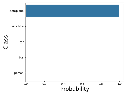
(b) Probabilities classifier Only the top 5 classes are displayed

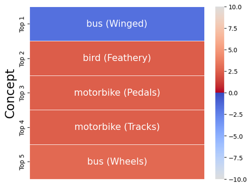
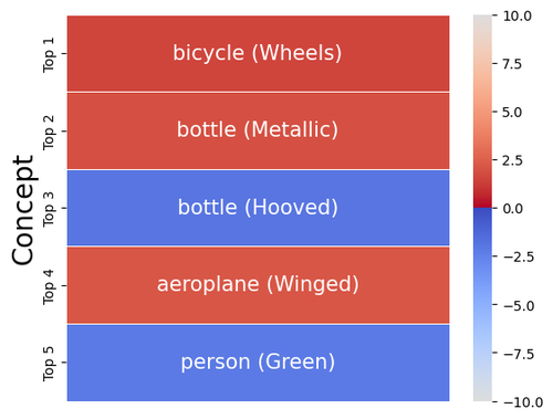
(c) Local explanation Only the top 5 classes are displayed

(d) Global explanation associated with the two highest probabilities. Here “aeroplane” and “motorbike”

Figure 12: Example of explanation on the PASCAL-Part dataset

(a) Input image

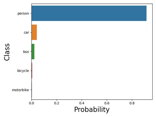
(b) Probabilities classifier Only the top 5 classes are displayed

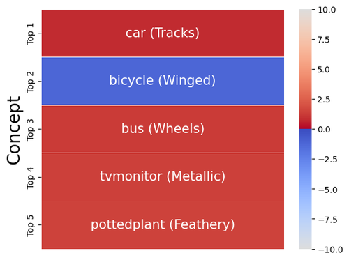
(c) Local explanation Only the top 5 classes are displayed

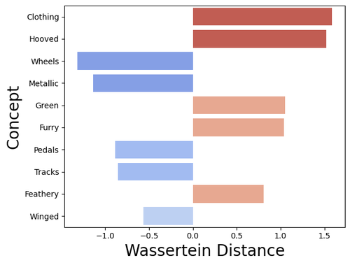
(d) Global explanation associated with the two highest probabilities. Here “potted plant” and “bottle”

Figure 13: Example of explanation on the PASCAL-Part dataset

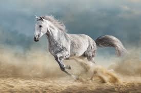
(a) Input image

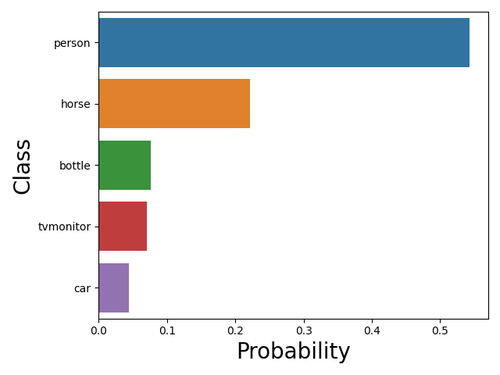
(b) Probabilities classifier Only the top 5 classes are displayed

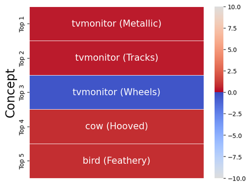
(c) Local explanation Only the top 5 classes are displayed

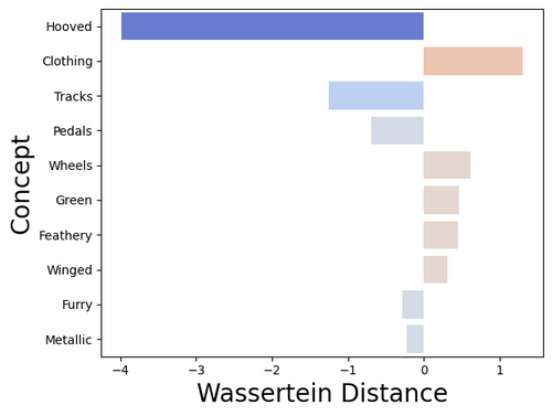
(d) Global explanation associated with the two highest probabilities. Here “person” and “car”

Figure 14: Example of explanation on the PASCAL-Part dataset

(a) Input image

(b) Probabilities classifier Only the top 5 classes are displayed

(c) Local explanation Only the top 5 classes are displayed

(d) Global explanation associated with the two highest probabilities. Here “person” and “horse”

Figure 15: Example of explanation on the PASCAL-Part dataset

References

- Akkus et al. (2023) Cem Akkus, Luyang Chu, Vladana Djakovic, Steffen Jauch-Walser, Philipp Koch, Giacomo Loss, Christopher Marquardt, Marco Moldovan, Nadja Sauter, Maximilian Schneider, et al. Multimodal deep learning. arXiv preprint arXiv:2301.04856, 2023.
- Arrieta et al. (2020) Alejandro Barredo Arrieta, Natalia Díaz-Rodríguez, Javier Del Ser, Adrien Bennetot, Siham Tabik, Alberto Barbado, Salvador García, Sergio Gil-López, Daniel Molina, Richard Benjamins, et al. Explainable artificial intelligence (XAI): Concepts, taxonomies, opportunities and challenges toward responsible AI. Information Fusion, 58:82–115, 2020.
- Bennetot et al. (2022) Adrien Bennetot, Gianni Franchi, Javier Del Ser, Raja Chatila, and Natalia Diaz-Rodriguez. Greybox XAI: A neural-symbolic learning framework to produce interpretable predictions for image classification. Knowledge-Based Systems, 258:109947, 2022.
- Brown et al. (2020) Tom Brown, Benjamin Mann, Nick Ryder, Melanie Subbiah, Jared D. Kaplan, Prafulla Dhariwal, Arvind Neelakantan, Pranav Shyam, Girish Sastry, Amanda Askell, et al. Language models are few-shot learners. Advances in Neural Information Processing Systems, 33:1877–1901, 2020.
- Chambers (2018) John M. Chambers. Graphical Methods for Data Analysis. CRC Press, 2018.
- Cortez & Embrechts (2011) Paulo Cortez and Mark J. Embrechts. Opening black box data mining models using sensitivity analysis. In 2011 IEEE Symposium on Computational Intelligence and Data Mining (CIDM), pp. 341–348. IEEE, 2011.
- Cukierski (2013) Will Cukierski. Dogs vs. cats, 2013. URL https://kaggle.com/competitions/dogs-vs-cats.
- Deng et al. (2009) Jia Deng, Wei Dong, Richard Socher, Li-Jia Li, Kai Li, and Li Fei-Fei. Imagenet: A large-scale hierarchical image database. In 2009 IEEE Conference on Computer Vision and Pattern Recognition, pp. 248–255, 2009.
- Donadello & Serafini (2016) Ivan Donadello and Luciano Serafini. Integration of numeric and symbolic information for semantic image interpretation. Intelligenza Artificiale, 10(1):33–47, 2016.
- Dosovitskiy et al. (2021) Alexey Dosovitskiy, Lucas Beyer, Alexander Kolesnikov, Dirk Weissenborn, Xiaohua Zhai, Thomas Unterthiner, Mostafa Dehghani, Matthias Minderer, Georg Heigold, Sylvain Gelly, et al. An image is worth 16x16 words: Transformers for image recognition at scale. In International Conference on Learning Representations, 2021.
- Feng et al. (2023) Zhili Feng, Anna Bair, and J. Zico Kolter. Leveraging multiple descriptive features for robust few-shot image learning. arXiv preprint arXiv:2307.04317, 2023.
- Galton (1886) Francis Galton. Regression towards mediocrity in hereditary stature. The Journal of the Anthropological Institute of Great Britain and Ireland, 15:246–263, 1886.
- Hastie et al. (2009) Trevor Hastie, Robert Tibshirani, and Jerome H. Friedman. The Elements of Statistical Learning: Data Mining, Inference, and Prediction, volume 2. Springer, 2009.
- He et al. (2016) Kaiming He, Xiangyu Zhang, Shaoqing Ren, and Jian Sun. Deep residual learning for image recognition. In Proceedings of the IEEE Conference on Computer Vision and Pattern Recognition, pp. 770–778, 2016.
- Johnson et al. (2016) Justin Johnson, Alexandre Alahi, and Li Fei-Fei. Perceptual losses for real-time style transfer and super-resolution. In Computer Vision–ECCV 2016: 14th European Conference, Amsterdam, The Netherlands, October 11-14, 2016, Proceedings, Part II 14, pp. 694–711. Springer, 2016.
- Kim et al. (2023) Siwon Kim, Jinoh Oh, Sungjin Lee, Seunghak Yu, Jaeyoung Do, and Tara Taghavi. Grounding counterfactual explanation of image classifiers to textual concept space. In Proceedings of the IEEE/CVF Conference on Computer Vision and Pattern Recognition, pp. 10942–10950, 2023.
- Koh et al. (2020) Pang Wei Koh, Thao Nguyen, Yew Siang Tang, Stephen Mussmann, Emma Pierson, Been Kim, and Percy Liang. Concept bottleneck models. In International Conference on Machine Learning, pp. 5338–5348, 2020.
- Krause et al. (2013) Jonathan Krause, Michael Stark, Jia Deng, and Li Fei-Fei. 3d object representations for fine-grained categorization. In 4th International IEEE Workshop on 3D Representation and Recognition (3dRR-13), Sydney, Australia, 2013.
- Kumar et al. (2009) Neeraj Kumar, Alexander C. Berg, Peter N. Belhumeur, and Shree K. Nayar. Attribute and simile classifiers for face verification. In 2009 IEEE 12th International Conference on Computer Vision, pp. 365–372. IEEE, 2009.
- Lamas et al. (2021) Alberto Lamas, Siham Tabik, Policarpo Cruz, Rosana Montes, Álvaro Martinez-Sevilla, Teresa Cruz, and Francisco Herrera. Monumai: Dataset, deep learning pipeline and citizen science based app for monumental heritage taxonomy and classification. Neurocomputing, 420:266–280, 2021.
- Lampert et al. (2009) Christoph H. Lampert, Hannes Nickisch, and Stefan Harmeling. Learning to detect unseen object classes by between-class attribute transfer. In 2009 IEEE Conference on Computer Vision and Pattern Recognition, pp. 951–958. IEEE, 2009.
- LeCun et al. (2015) Yann LeCun, Yoshua Bengio, and Geoffrey Hinton. Deep learning. Nature, 521(7553):436–444, 2015.
- Liu et al. (2020) Xiaodong Liu, Kevin Duh, Liyuan Liu, and Jianfeng Gao. Very deep transformers for neural machine translation. arXiv preprint arXiv:2008.07772, 2020.
- Losch et al. (2019) Max Losch, Mario Fritz, and Bernt Schiele. Interpretability beyond classification output: Semantic bottleneck networks. arXiv preprint arXiv:1907.10882, 2019.
- Lundberg & Lee (2017) Scott M. Lundberg and Su-In Lee. A unified approach to interpreting model predictions. Advances in Neural Information Processing Systems, 30, 2017.
- Luo et al. (2022) Huaishao Luo, Lei Ji, Ming Zhong, Yang Chen, Wen Lei, Nan Duan, and Tianrui Li. Clip4clip: An empirical study of clip for end to end video clip retrieval and captioning. Neurocomputing, 508:293–304, 2022.
- Luo et al. (2023) Jinqi Luo, Zhaoning Wang, Chen Henry Wu, Dong Huang, and Fernando De la Torre. Zero-shot model diagnosis. In Proceedings of the IEEE/CVF Conference on Computer Vision and Pattern Recognition, pp. 11631–11640, 2023.
- Mahalanobis (2018) Prasanta Chandra Mahalanobis. On the generalized distance in statistics. Sankhyā: The Indian Journal of Statistics, Series A (2008-), 80:S1–S7, 2018.
- McCullagh (2019) Peter McCullagh. Generalized Linear Models. Routledge, 2019.
- Menon & Vondrick (2022) Sachit Menon and Carl Vondrick. Visual classification via description from large language models. In The Eleventh International Conference on Learning Representations, 2022.
- Nilsback & Zisserman (2008) Maria-Elena Nilsback and Andrew Zisserman. Automated flower classification over a large number of classes. In Indian Conference on Computer Vision, Graphics and Image Processing, 12 2008.
- Oikarinen et al. (2023) Tuomas Oikarinen, Subhro Das, Lam Nguyen, and Lily Weng. Label-free concept bottleneck models. In International Conference on Learning Representations, 2023.
- Ouyang et al. (2022) Long Ouyang, Jeffrey Wu, Xu Jiang, Diogo Almeida, Carroll Wainwright, Pamela Mishkin, Chong Zhang, Sandhini Agarwal, Katarina Slama, Alex Ray, et al. Training language models to follow instructions with human feedback. Advances in Neural Information Processing Systems, 35:27730–27744, 2022.
- Panousis et al. (2023) Konstantinos P. Panousis, Dino Ienco, and Diego Marcos. Sparse linear concept discovery models. In Proceedings of the IEEE/CVF International Conference on Computer Vision, pp. 2767–2771, 2023.
- Peters et al. (2017) Jonas Peters, Dominik Janzing, and Bernhard Schölkopf. Elements of Causal Inference: Foundations and Learning Algorithms. The MIT Press, 2017.
- Petsiuk et al. (2018) Vitali Petsiuk, Abir Das, and Kate Saenko. RISE: Randomized input sampling for explanation of black-box models. arXiv preprint arXiv:1806.07421, 2018.
- Plumb et al. (2018) Gregory Plumb, Denali Molitor, and Ameet S Talwalkar. Model agnostic supervised local explanations. Advances in neural information processing systems, 31, 2018.
- Plumb et al. (2022) Gregory Plumb, Marco Tulio Ribeiro, and Ameet Talwalkar. Finding and fixing spurious patterns with explanations. Transactions on Machine Learning Research, 2022. ISSN 2835-8856. URL https://openreview.net/forum?id=whJPugmP5I. Expert Certification.
- Quattoni & Torralba (2009) Ariadna Quattoni and Antonio Torralba. Recognizing indoor scenes. In 2009 IEEE Conference on Computer Vision and Pattern Recognition, pp. 413–420. IEEE, 2009.
- Quinlan (1986) J. Ross Quinlan. Induction of decision trees. Machine Learning, 1:81–106, 1986.
- Radford et al. (2021) Alec Radford, Jong Wook Kim, Chris Hallacy, Aditya Ramesh, Gabriel Goh, Sandhini Agarwal, Girish Sastry, Amanda Askell, Pamela Mishkin, Jack Clark, et al. Learning transferable visual models from natural language supervision. In International Conference on Machine Learning, pp. 8748–8763, 2021.
- Ramesh et al. (2021) Aditya Ramesh, Mikhail Pavlov, Gabriel Goh, Scott Gray, Chelsea Voss, Alec Radford, Mark Chen, and Ilya Sutskever. Zero-shot text-to-image generation. In International Conference on Machine Learning, pp. 8821–8831, 2021.
- Reed et al. (2022) Scott Reed, Konrad Zolna, Emilio Parisotto, Sergio Gómez Colmenarejo, Alexander Novikov, Gabriel Barth-maron, Mai Giménez, Yury Sulsky, Jackie Kay, Jost Tobias Springenberg, et al. A generalist agent. Transactions on Machine Learning Research, 2022.
- Ribeiro et al. (2016) Marco Tulio Ribeiro, Sameer Singh, and Carlos Guestrin. “Why should I trust you?”: Explaining the predictions of any classifier. In Proceedings of the 22nd ACM SIGKDD International Conference on Knowledge Discovery and Data Mining, San Francisco, CA, USA, August 13-17, 2016, pp. 1135–1144, 2016.
- Rombach et al. (2021) Robin Rombach, Andreas Blattmann, Dominik Lorenz, Patrick Esser, and Björn Ommer. High-resolution image synthesis with latent diffusion models. In CVF Conference on Computer Vision and Pattern Recognition (CVPR), pp. 10674–10685, 2021.
- Schuhmann et al. (2022) Christoph Schuhmann, Romain Beaumont, Richard Vencu, Cade Gordon, Ross Wightman, Mehdi Cherti, Theo Coombes, Aarush Katta, Clayton Mullis, Mitchell Wortsman, et al. Laion-5b: An open large-scale dataset for training next generation image-text models. Advances in Neural Information Processing Systems, 35:25278–25294, 2022.
- Selvaraju et al. (2017) Ramprasaath R. Selvaraju, Michael Cogswell, Abhishek Das, Ramakrishna Vedantam, Devi Parikh, and Dhruv Batra. Grad-cam: Visual explanations from deep networks via gradient-based localization. In Proceedings of the IEEE International Conference on Computer Vision, pp. 618–626, 2017.
- Tommasi et al. (2017) Tatiana Tommasi, Novi Patricia, Barbara Caputo, and Tinne Tuytelaars. A deeper look at dataset bias. Domain Adaptation in Computer Vision Applications, pp. 37–55, 2017.
- Yan et al. (2023a) An Yan, Yu Wang, Yiwu Zhong, Chengyu Dong, Zexue He, Yujie Lu, William Yang Wang, Jingbo Shang, and Julian McAuley. Learning concise and descriptive attributes for visual recognition. In Proceedings of the IEEE/CVF International Conference on Computer Vision, pp. 3090–3100, 2023a.
- Yan et al. (2023b) An Yan, Yu Wang, Yiwu Zhong, Zexue He, Petros Karypis, Zihan Wang, Chengyu Dong, Amilcare Gentili, Chun-Nan Hsu, Jingbo Shang, et al. Robust and interpretable medical image classifiers via concept bottleneck models. arXiv preprint arXiv:2310.03182, 2023b.
- Yang et al. (2023) Yue Yang, Artemis Panagopoulou, Shenghao Zhou, Daniel Jin, Chris Callison-Burch, and Mark Yatskar. Language in a bottle: Language model guided concept bottlenecks for interpretable image classification. In Proceedings of the IEEE/CVF Conference on Computer Vision and Pattern Recognition, pp. 19187–19197, 2023.
- Yuksekgonul et al. (2022) Mert Yuksekgonul, Maggie Wang, and James Zou. Post-hoc concept bottleneck models. In The Eleventh International Conference on Learning Representations, 2022.