Fast ODE-based Sampling for Diffusion Models in Around 5 Steps

Abstract

Sampling from diffusion models can be treated as solving the corresponding ordinary differential equations (ODEs), with the aim of obtaining an accurate solution with as few number of function evaluations (NFE) as possible. Recently, various fast samplers utilizing higher-order ODE solvers have emerged and achieved better performance than the initial first-order one. However, these numerical methods inherently result in certain approximation errors, which significantly degrades sample quality with extremely small NFE (e.g., around 5). In contrast, based on the geometric observation that each sampling trajectory almost lies in a two-dimensional subspace embedded in the ambient space, we propose Approximate MEan-Direction Solver (AMED-Solver) that eliminates truncation errors by directly learning the mean direction for fast diffusion sampling. Besides, our method can be easily used as a plugin to further improve existing ODE-based samplers. Extensive experiments on image synthesis with the resolution ranging from 32 to 256 demonstrate the effectiveness of our method. With only 5 NFE, we achieve 7.14 FID on CIFAR-10, 13.75 FID on ImageNet 64$\times$64, and 12.79 FID on LSUN Bedroom. Our code is available at https://github.com/zhyzhouu/amed-solver.

1 Introduction

Diffusion models have been attracting growing attentions in recent years due to their impressive generative capability [9, 31, 35, 33]. Given a noise input, they are able to generate a realistic output by performing iterative denoising steps with the score function [39, 15, 42]. This process can be interpreted as applying a certain numerical discretization on a stochastic differential equation (SDE), or more commonly, its corresponding probability flow ordinary differential equation (PF-ODE) [42]. Comparing to other generative models such as GANs [12] and VAEs [19], diffusion models have the advantages in high sample quality and stable training, but suffer from slow sampling speed, which poses a great challenge to their applications.

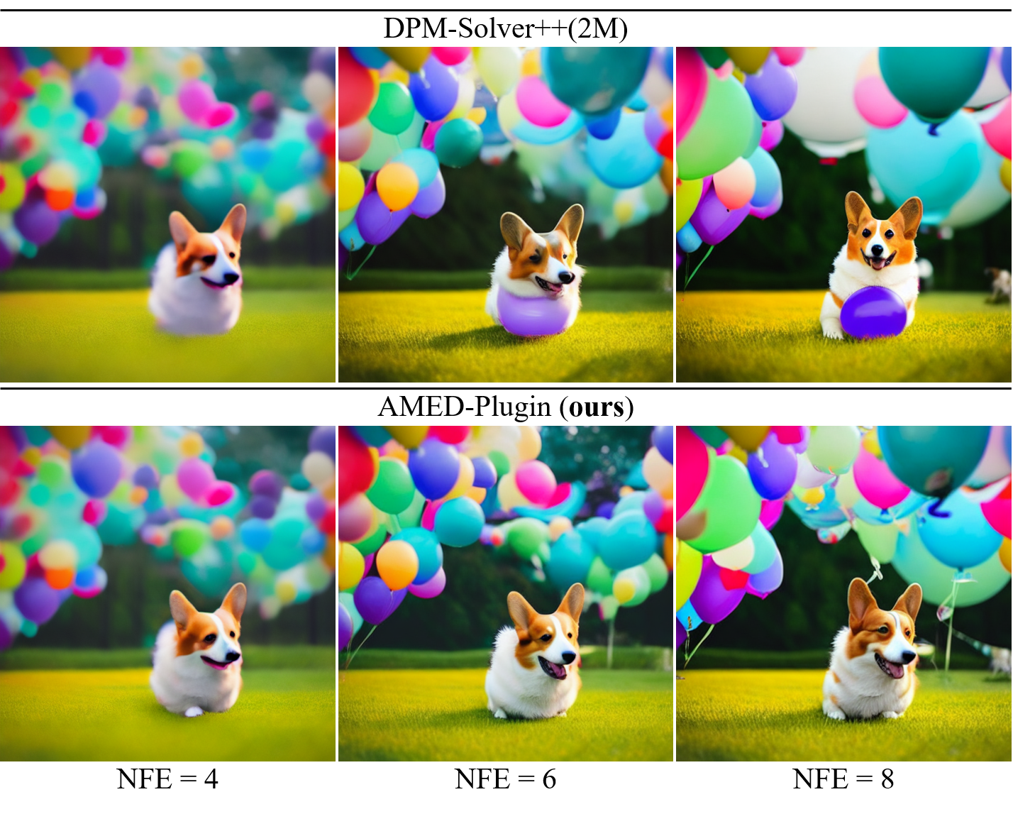
Figure 1: Synthesized images by Stable-Diffusion [31] with a default classifier-free guidance scale 7.5 and a text prompt “A Corgi on the grass surrounded by a cluster of colorful balloons”. Our method improves DPM-Solver++(2M) [25] in sample quality.

Existing methods for accelerating diffusion sampling fall into two main streams. One is designing faster numerical solvers to increase step size while maintaining small truncation errors [40, 22, 24, 47, 18, 10]. They can be further categorized as single-step solvers and multi-step solvers [2]. The former computes the next step solution only using information from the current time step, while the latter uses multiple past time steps. These methods have successfully reduced the number of function evaluations (NFE) from 1000 to less than 20, almost without affecting the sample quality.

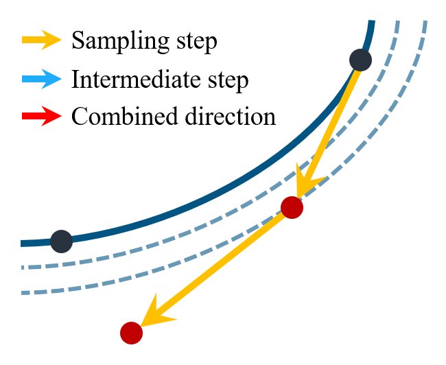
(a) DDIM solver.

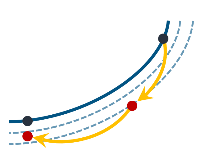
(b) Multi-step solvers.

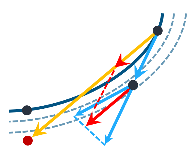
(c) Generalized DPM-Solver-2.

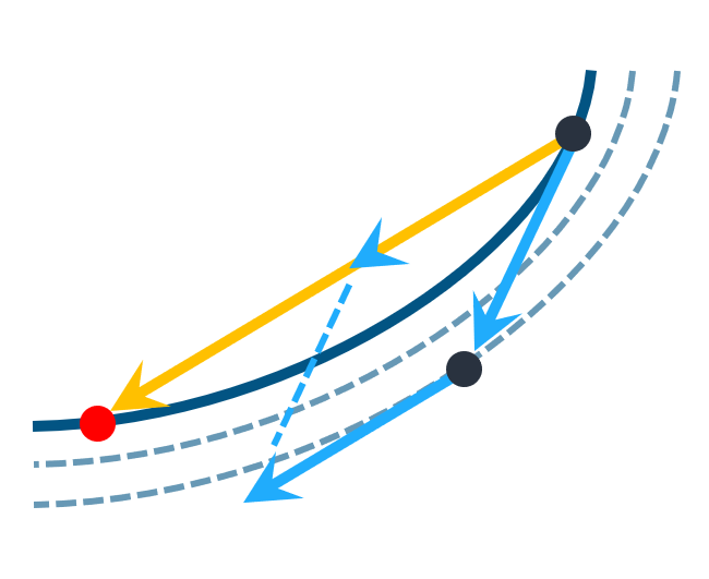
(d) AMED-Solver (ours).

Figure 2: Comparison of various ODE solvers. Red dots depict the actual sampling step of different solvers. (a) DDIM solver [40] applies Euler discretization on PF-ODEs. In every sampling step, it follows the gradient direction to give the solution for next time step. (b) Multi-step solvers [22, 47, 25, 48] require current gradient and several records of history gradients and then follow the combination of these gradients to give the solution. (c) In generalized DPM-Solver-2 [24], there is a hyper-parameter $r$ controlling the location of intermediate time step. $r=0.5$ recovers the default DPM-Solver-2 and $r=1$ recovers Heun’s second method [18]. The gradient for sampling step is given by the combination of gradients at intermediate and current time steps (see Tab. 1). (d) Our proposed AMED-Solver seeks to find the intermediate time step that gives nearly optimal gradient directing to the ground truth solution. This gradient used for sampling step is adaptively learned instead of the heuristic assigned as DPM-Solver-2.

Another kind of methods aim to build a one-to-one mapping between the data distribution and the pre-specified noise distribution [26, 36, 23, 43, 4], based on the idea of knowledge distillation. With a well-trained student model in hand, high-quality generation can be achieved with only one NFE. However, training such a student model either requires pre-generation of millions of images [26, 23], or huge training cost with carefully modified training procedure [36, 43, 4]. Besides, distillation-based models cannot guarantee the increase of sample quality given more NFE and they have difficulty in likelihood evaluation.

In this paper, we further boost ODE-based sampling for diffusion models in around 5 steps. Based on the geometric property that each sampling trajectory approximately lies on a two-dimensional subspace embedded in the high-dimension space, we propose Approximate MEan-Direction Solver (AMED-Solver), a single-step ODE solver that learns to predict the optimal intermediate time step in every sampling step. A comparison of various ODE solvers is illustrated in Fig. 2. We also extend our method to any ODE solvers as a plugin. Based on the previous observation that the sampling trajectory generated by diffusion models is nearly straight [6], we perform analytical first step (AFS) [10] to save one NFE almost without affecting the sample quality. When applying AMED-Plugin on the improved PNDM method, we achieve FID of 7.14 on CIFAR-10, 13.75 on ImageNet 64$\times$64, and 12.79 on LSUN Bedroom. Our main contributions are as follows:

• We introduce AMED-Solver, a new single-step ODE solver for diffusion models that eliminates truncation errors by design.

• We propose AMED-Plugin that can be applied to any ODE solvers with a small training overhead and a negligible sampling overhead.

• Extensive experiments on various datasets validate the effectiveness of our method in fast image generation.

2 Background

2.1 Diffusion Models

The forward diffusion process can be formalized as a SDE:

$$\mathrm{d}\mathbf{x}=\mathbf{f}(\mathbf{x},t)\mathrm{d}t+g(t)\mathrm{d}\mathbf{w}_{t},$$ (1)

where $\mathbf{f}(\cdot,t):\mathbb{R}^{d}\rightarrow\mathbb{R}^{d},g(\cdot):\mathbb{R}\rightarrow\mathbb{R}$ are drift and diffusion coefficients, respectively, and $\mathbf{w}_{t}\in\mathbb{R}^{d}$ is the standard Wiener process [29]. This forward process forms a continuous stochastic process $\{\mathbf{x}_{t}\}_{t=0}^{T}$ and the associated probability density $\{p_{t}(\mathbf{x})\}_{t=0}^{T}$, to make the sample $\mathbf{x}_{0}$ from the implicit data distribution $p_{d}=p_{0}$ approximately distribute as the pre-specified noise distribution, i.e., $p_{T}\approx p_{n}$. Given an encoding $\mathbf{x}_{T}\sim p_{n}$, generation is then performed with the reversal of Eq. 1 [11, 1]. Remarkably, there exists a probability flow ODE (PF-ODE)

$$\mathrm{d}\mathbf{x}=\left[\mathbf{f}(\mathbf{x},t)-\frac{1}{2}g(t)^{2}\nabla_{\mathbf{x}}\log p_{t}(\mathbf{x})\right]\mathrm{d}t,$$ (2)

sharing the same marginals with the reverse SDE [27, 42], and $\nabla_{\mathbf{x}}\log p_{t}(\mathbf{x})$ is known as the score function [16]. Generally, this PF-ODE is preferred in practice for its conceptual simplicity, sampling efficiency and unique encoding [42]. Throughout this paper, we follow the configuration of EDM [18] by setting $\mathbf{f}(\mathbf{x},t)=\mathbf{0}$, $g(t)=\sqrt{2t}$ and $\sigma(t)=t$. In this case, the reciprocal of $t^{2}$ equals to the signal-to-noise ratio [20] and the perturbation kernel is

$$p_{t}(\mathbf{x}|\mathbf{x}_{0})=\mathcal{N}(\mathbf{x};\mathbf{x}_{0},t^{2}\mathbf{I}).$$ (3)

To simulate the PF-ODE, we usually train a U-Net [32, 15] predicting $\mathbf{s}_{\theta}(\mathbf{x},t)$ to approximate the intractable $\nabla_{\mathbf{x}}\log p_{t}(\mathbf{x})$. There are mainly two parameterizations in the literature. One uses a noise prediction model $\boldsymbol{\epsilon}_{\theta}(\mathbf{x},t)$ predicting the Gaussian noise added to $\mathbf{x}$ at time $t$ [15, 40], and another uses a data prediction model $\mathbf{D}_{\theta}(\mathbf{x},t)$ predicting the denoising output of $\mathbf{x}$ from time $t$ to $0$ [18, 25, 6]. They have the following relationship in our setting:

$$\mathbf{s}_{\theta}(\mathbf{x},t)=-\frac{\boldsymbol{\epsilon}_{\theta}(\mathbf{x},t)}{t}=\frac{\mathbf{D}_{\theta}(\mathbf{x},t)-\mathbf{x}}{t^{2}}.$$ (4)

The training of diffusion models in the noise prediction notation is performed by minimizing a weighted combination of the least squares estimations:

$$\mathbb{E}_{\mathbf{x}\sim p_{d},\mathbf{z}\sim\mathcal{N}(\mathbf{0},t^{2}\mathbf{I})}\lVert\boldsymbol{\epsilon}_{\boldsymbol{\theta}}(\mathbf{x}+\mathbf{z};t)-\boldsymbol{\epsilon}\rVert^{2}_{2}.$$ (5)

We then plug the learned score function Eq. 4 into Eq. 2 to obtain a simple formulation for the PF-ODE

$$\mathrm{d}\mathbf{x}=\boldsymbol{\epsilon}_{\theta}(\mathbf{x},t)\mathrm{d}t.$$ (6)

The sampling trajectory $\{x_{t_{n}}\}_{n=1}^{N}$ is obtained by first draw $\mathbf{x}_{t_{N}}\sim p_{n}=\mathcal{N}(\mathbf{0},T^{2}\mathbf{I})$ and then solve Eq. 6 with $N-1$ steps following time schedule $\Gamma=\{t_{1}=\epsilon,\cdots,t_{N}=T\}$.

2.2 Categorization of Previous Fast ODE Solvers

To accelerate diffusion sampling, various fast ODE solvers have been proposed, which can be classified into single-step solvers or multi-step solvers [2]. Single-step solvers including DDIM [40], EDM [18] and DPM-Solver [24] which only use the information from the current time step to compute the solution for the next time step, while multi-step solvers including PNDM [22] and DEIS [47] utilize multiple past time steps to compute the next time step (see Fig. 2 for an intuitive comparison). We emphasize that one should differ single-step ODE solvers from single-step (NFE=1) distillation-based methods [26, 36, 43].

The advantages of single-step methods lie in the easy implementation and the ability to self-start since no history record is required. However, as illustrated in Fig. 3, they suffer from fast degradation of sample quality especially when the NFE budget is limited. The reason may be that the actual sampling steps of multi-step solvers are twice as much as those of single-step solvers with the same NFE, enabling them to adjust directions more frequently and flexibly. We will show that our proposed AMED-Solver can largely fix this issue with learned intermediate time steps.

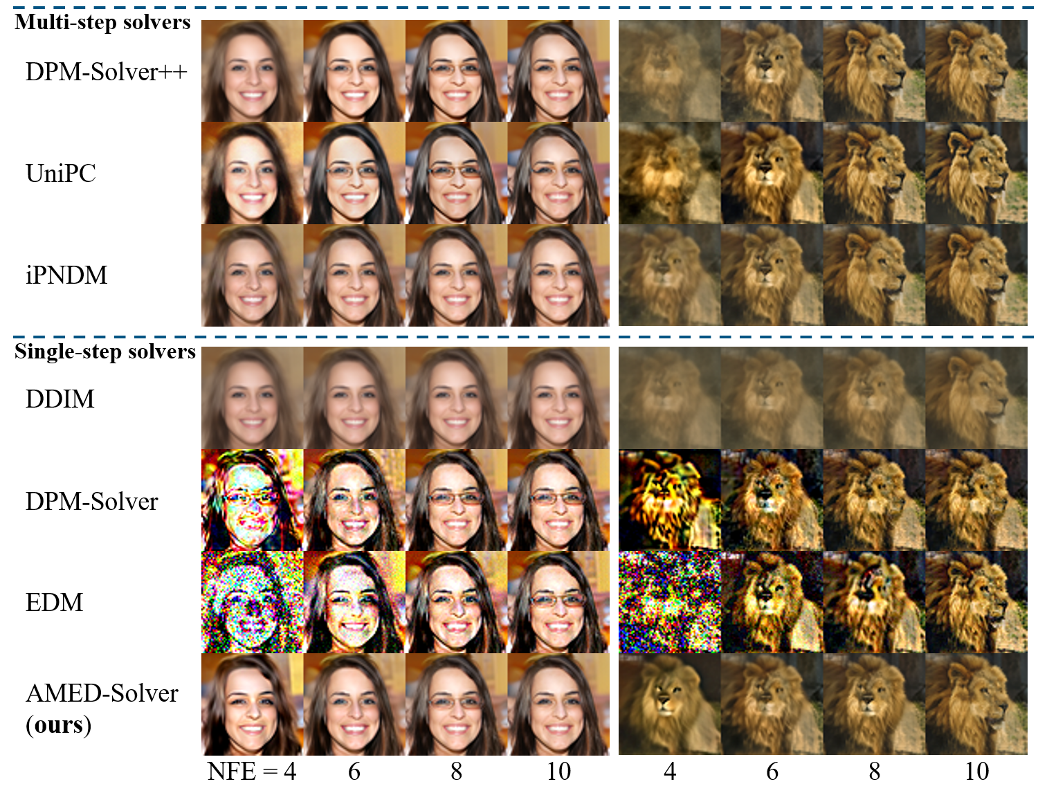
Figure 3: The sample quality degradation of multi-step and single-step ODE solvers. The quality of images generated by single-step solvers, especially higher-order ones including DPM-Solver-2 [24] and EDM [18], rapidly decreases as NFE decreases, while our proposed AMED-Solver largely mitigates such degradation. Examples are from FFHQ 64$\times$64 [17] and ImageNet 64$\times$64 [34].

Method	Gradient term	Source of $s_{n}$
DDIM [40]	$\boldsymbol{\epsilon}_{\theta}(\mathbf{x}_{t_{n+1}},t_{n+1})$	-
EDM [18]	$\frac{1}{2}\boldsymbol{\epsilon}_{\theta}(\mathbf{x}_{s_{n}},s_{n})+\frac{1}{2}\boldsymbol{\epsilon}_{\theta}(\mathbf{x}_{t_{n+1}},t_{n+1})$	$t_{n}$
DPM-Solver-2 [24]	$\frac{1}{2r}\boldsymbol{\epsilon}_{\theta}(\mathbf{x}_{s_{n}},s_{n})+(1-\frac{1}{2r})\boldsymbol{\epsilon}_{\theta}(\mathbf{x}_{t_{n+1}},t_{n+1})$	$t_{n}^{r}t_{n+1}^{1-r}$, $r\in(0,1)$
AMED-Solver	$\boldsymbol{\epsilon}_{\theta}(\mathbf{x}_{s_{n}},s_{n})$	Learned

Table 1: Comparison of various single-step ODE solvers.

3 Our Proposed AMED-Solver

In this section, we propose AMED-Solver, a single-step ODE solver for diffusion models that releases the potential of single-step solvers in extremely small NFE, enabling them to match or even surpass the performance of multi-step solvers. Furthermore, our proposed method can be generalized as a plugin on any ODE solver, yielding promising improvement across various datasets. Our key observation is that the sampling trajectory generated by Eq. 6 nearly lies in a two-dimensional subspace embedded in high-dimensional space, which motivates us to minimize the discretization error with the mean value theorem.

3.1 The Sampling Trajectory Almost Lies in a Two-Dimensional Subspace

The sampling trajectory generated by solving Eq. 6 exhibits an extremely simple geometric structure and has an implicit connection to the annealed mean shift, as revealed in the previous work [6]. Each sample starting from the noise distribution approaches the data manifold along a smooth, quasi-linear sampling trajectory in a monotone likelihood increasing way [6]. Besides, all trajectories from different initial points share the similar geometric shape, whether in the conditional or unconditional generation case.

In this paper, we further point out that the sampling trajectory generated by ODE solvers almost lies in a two-dimensional plane embedded in a high-dimensional space. We experimentally validate this claim by performing Principal Component Analysis (PCA) for 1k sampling trajectories on different datasets including CIFAR10 32$\times$32 [21], FFHQ 64$\times$64 [17], ImageNet 64$\times$64 [34] and LSUN Bedroom 256$\times$256 [46]. As illustrated in Fig. 4, the relative projection error using two principal components is no more than 8$\%$ and always stays in a small level. Besides, the sample variance can be fully explained using only two principal components. Given the vast image space with dimensions of 3072(=3$\times 32\times 32$), 12288(=3$\times 64\times 64$), or 196608(=3$\times 256\times 256$), the sampling trajectories show intriguing property that their dynamics can almost be described using only two principal components.

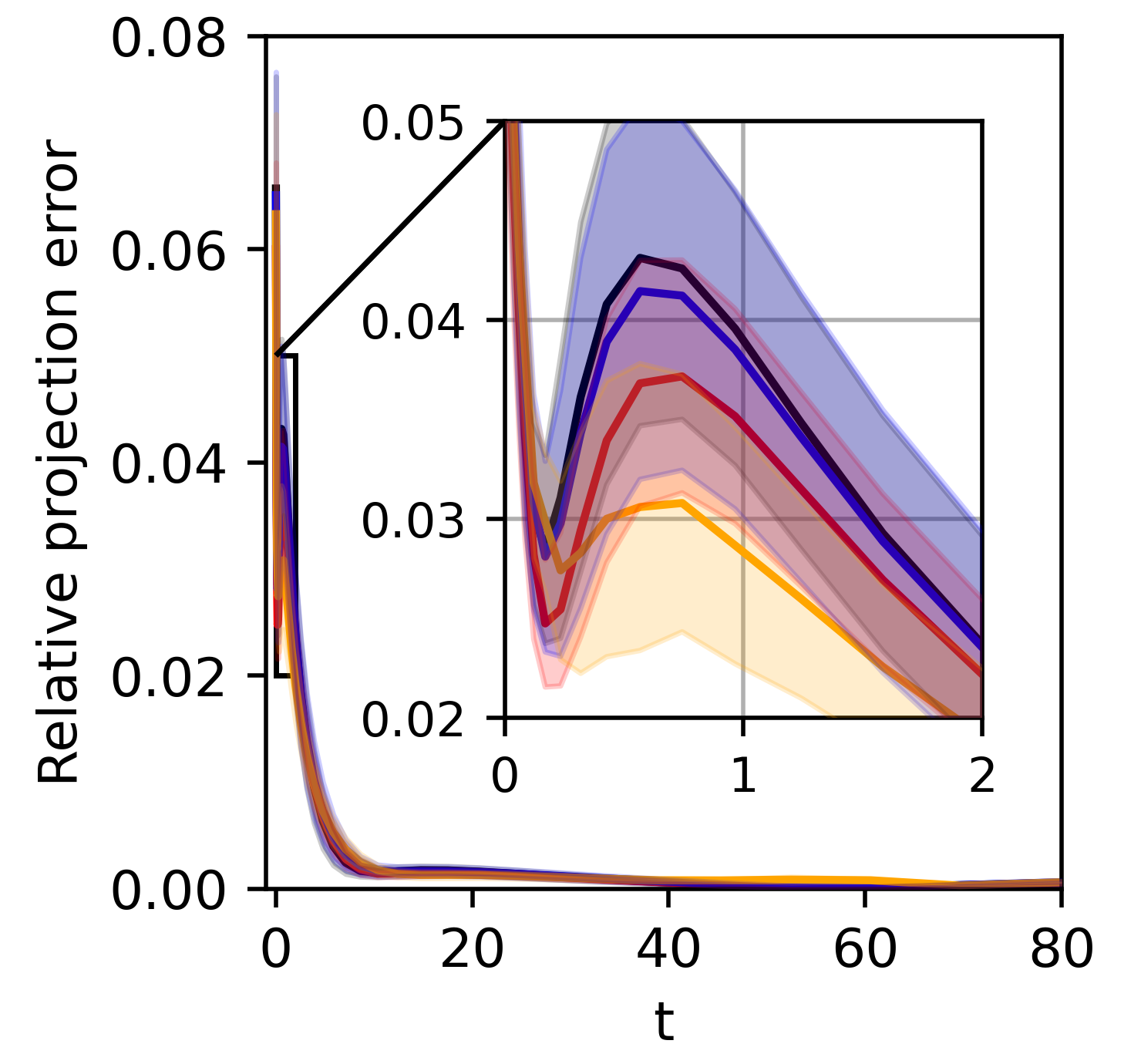
(a) Relative deviation.

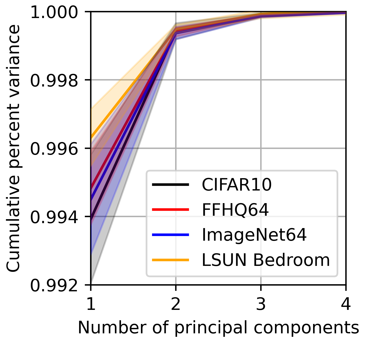
(b) Variance explained by top PCs.

Figure 4: We perform PCA to each sampling trajectory $\{x_{t}\}_{t=\epsilon}^{T}$. (a) These trajectories are projected into a 2D subspace spanned by the top 2 principal components to get $\{\tilde{x}_{t}\}_{t=\epsilon}^{T}$ and the relative projection error is calculated as $\left\|x_{t}-\tilde{x}_{t}\right\|_{2}/\left\|x_{t}\right\|_{2}$. (b) We progressively increase the number of principal components and calculate the cumulative percent variance as $\mathrm{Var}(\{\tilde{x}_{t}\}_{t=\epsilon}^{T})/\mathrm{Var}(\{x_{t}\}_{t=\epsilon}^{T})$. The results are obtained by averaging 1k sampling trajectories using EDM sampler [18] with 80 NFE.

3.2 Approximate Mean-Direction Solver

With the geometric intuition, we next explain our methods in more detail. The exact solution of Eq. 6 is:

$$\mathbf{x}_{t_{n}}=\mathbf{x}_{t_{n+1}}+\int_{t_{n+1}}^{t_{n}}\boldsymbol{\epsilon}_{\theta}(\mathbf{x}_{t},t)\mathrm{d}t.$$ (7)

Various numerical approximations to the integral above correspond to different types of fast ODE-based samplers. For instance, direct explicit rectangle method gives DDIM [40], linear multi-step method yields PNDM [22], Taylor expansion yields DPM-Solver [24] and polynomial extrapolation recovers DEIS [47]. Different from these works, we derive our method more directly by expecting that the mean value theorem holds for the integral involved so that we can find an intermediate time step $s_{n}\in\left(t_{n},t_{n+1}\right)$ with

$$\boldsymbol{\epsilon}_{\theta}(\mathbf{x}_{s_{n}},s_{n})=\frac{1}{t_{n}-t_{n+1}}\int_{t_{n+1}}^{t_{n}}\boldsymbol{\epsilon}_{\theta}(\mathbf{x}_{t},t)\mathrm{d}t.$$ (8)

Although the well-known mean value theorem for real-valued functions does not hold in vector-valued case [7], the remarkable geometric property that the sampling trajectory $\{x_{t}\}_{t=\epsilon}^{T}$ almost lies in a two-dimensional subspace guarantees our use. By choosing the intermediate time step, we are able to achieve an approximation of Eq. 7 by

$$\mathbf{x}_{t_{n}}\approx\mathbf{x}_{t_{n+1}}+(t_{n}-t_{n+1})\boldsymbol{\epsilon}_{\theta}(\mathbf{x}_{s_{n}},s_{n}).$$ (9)

The formulation above is actually a single-step ODE solver. The typical DPM-Solver-2 [24] can be recovered by setting $s_{n}=\sqrt{t_{n}t_{n+1}}$. In Tab. 1, we compare various single-step solvers by generalizing $\boldsymbol{\epsilon}_{\theta}(\mathbf{x}_{s_{n}},s_{n})$ as the gradient term.

For the choose of intermediate time steps, we train a shallow neural network $g_{\phi}$ based on distillation with small training and negligible sampling costs. Briefly, given samples $y_{t_{n}},y_{t_{n+1}}$ on the teacher sampling trajectory with higher NFE budget and $x_{t_{n+1}}$ on the student sampling trajectory, $g_{\phi}$ gives the intermediate time step $s_{n}$ that minimizes $d\left(x_{t_{n}},y_{t_{n}}\right)$ where $x_{t_{n}}$ is given by Eq. 9 and $d$ is a distance metric. Since we seek to find a mean-direction that best approximates the integral in Eq. 8, we name our proposed single-step ODE solver Eq. 9 Approximate MEan-Direction Solver, dubbed as AMED-Solver. Before specifying the training and sampling details, we proceed to generalize our idea to any fast ODE solvers.

3.3 AMED as A Plugin

The idea of AMED can be used to further improve existing fast ODE solvers for diffusion models. Throughout the paper, we adapt the polynomial time schedule [18]:

$$t_{n}=(t_{1}^{1/\rho}+\frac{n-1}{N-1}(t_{N}^{1/\rho}-t_{1}^{1/\rho}))^{\rho}.$$ (10)

Note that another usually used uniform logSNR schedule is actually the limit of Eq. 10 as $\rho$ approaches $+\infty$.

Given a time schedule $\Gamma=\{t_{1}=\epsilon,\cdots,t_{N}=T\}$, the AMED-Solver is obtained by performing extra model evaluations at $s_{n}\in(t_{n},t_{n+1}),n=1,\cdots,N-1$. Under the same manner, we are able to improve any ODE solvers by predicting $\{s_{n}\}_{n=1}^{N-1}$ that best aligns the student and teacher sampling trajectories.

We validate this by an experiment where we first generate a ground truth trajectory using Heun’s second method with 80 NFE and extract samples at $\Gamma$ to get $\{x_{t_{n}}^{G}\}_{n=1}^{N}$. For every ODE solver, we generate a baseline trajectory $\{x_{t_{n}}^{B}\}_{n=1}^{N}$ by performing evaluations at $s_{n}=\sqrt{t_{n}t_{n+1}}$ following the original time schedule. We then apply a grid search on $r_{n}$, giving $s_{n}=t_{n}^{r_{n}}t_{n+1}^{1-{r_{n}}}$ and a searched trajectory $\{x_{t_{n}}^{S}\}_{n=1}^{N}$. We define the relative alignment to be $\left\|x_{t_{n}}^{B}-x_{t_{n}}^{G}\right\|_{2}-\left\|x_{t_{n}}^{S}-x_{t_{n}}^{G}\right\|_{2}$. As shown in Fig. 5, the relative alignment keeps positive in most cases, meaning that appropriate choose of intermediate time steps can further improve fast ODE solvers. Therefore, as described in Sec. 3.2, we can also train a neural network to appropriately predict intermediate time steps. As this process still has the meaning of searching for the direction pointing to the ground truth, we name this method as AMED-Plugin and apply it on various fast ODE solvers.

Through Fig. 5, we obtain a direct comparison between DPM-Solver-2 and our proposed AMED-Solver since they share the same baseline trajectory when $r$ is fixed to $0.5$. The AMED-Solver provides better alignment to the ground truth and the location of searched intermediate time steps is much more stable than that of DPM-Solver-2. We speculate that for DPM-Solver-2, the direction of gradient term is restricted by the combination where the coefficients is fixed by $r$ (see Tab. 1). Instead, the gradient term of AMED-Solver is directly given by the intermediate time step, providing more flexibility than DPM-Solver-2.

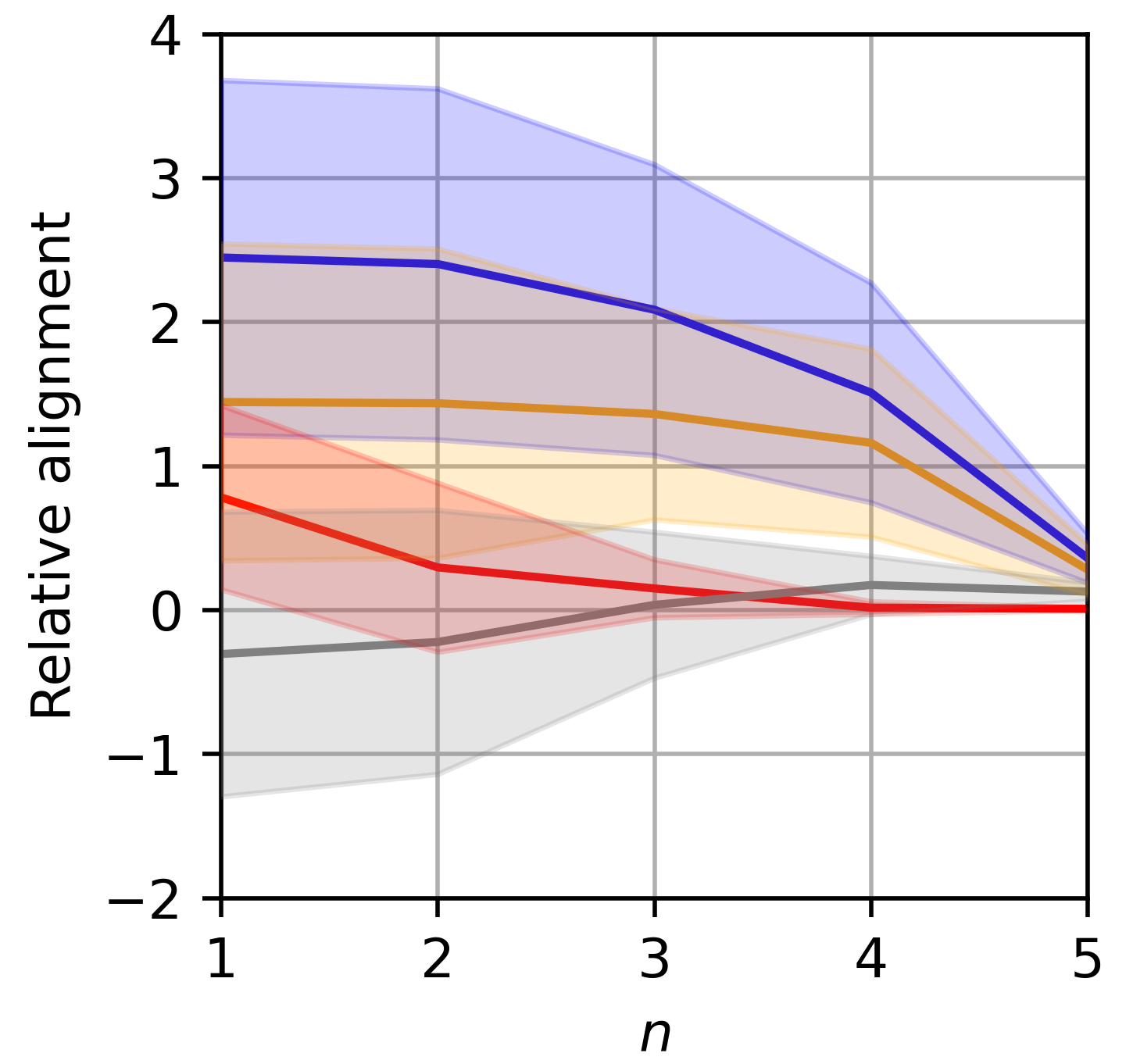
(a) Relative alignment at time $t_{n}$.

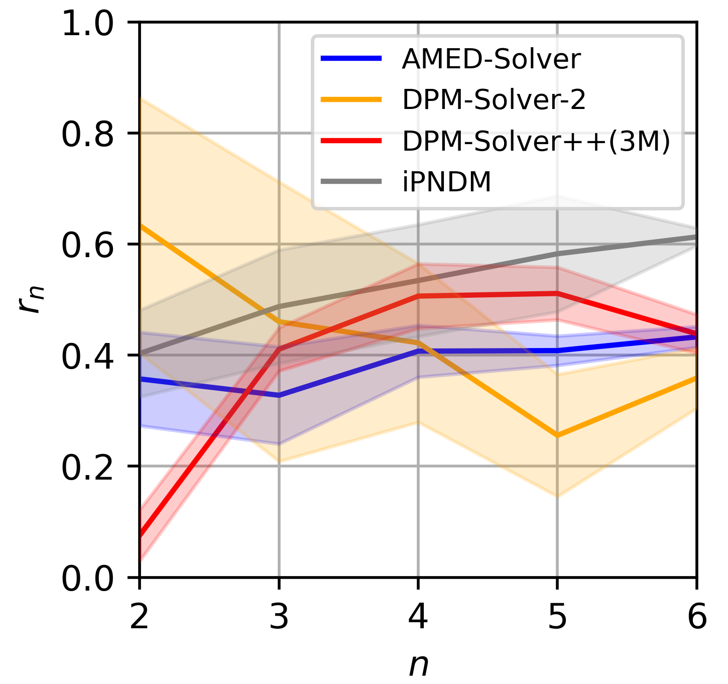
(b) Best $r_{n}$s given by grid search.

Figure 5: Effectiveness of searching the intermediate time steps. Given schedule $\Gamma=\{t_{1}=\epsilon,\cdots,t_{N}=T\}$ where $\epsilon=0.002,T=80,N=6$, we first generate a ground truth trajectory. For every ODE solver involved, we generate a baseline trajectory by performing evaluations at $s_{n}=\sqrt{t_{n}t_{n+1}}$, and a searched trajectory by a greedy grid search on $r_{n}$ which gives $s_{n}=t_{n}^{r_{n}}t_{n+1}^{1-{r_{n}}}$.

3.4 Training and Sampling

As samples from different sampling trajectories approach the asymmetric data manifold from different directions, the location of current points should contribute to the shape of the sampling trajectories. To recognize the location of one sample without extra computation overhead, we extract the bottleneck feature of the pre-trained U-Net model every time after its evaluation. We then take the current time step $t_{n+1}$ along with the bottleneck feature $h_{t_{n+1}}$ as the inputs of the shallow neural network $g_{\phi}$ to predict the intermediate time step $s_{n}$. Formally, we have

$$s_{n}=g_{\phi}(h_{t_{n+1}},t_{n+1}).$$ (11)

The network architecture is shown in Fig. 6.

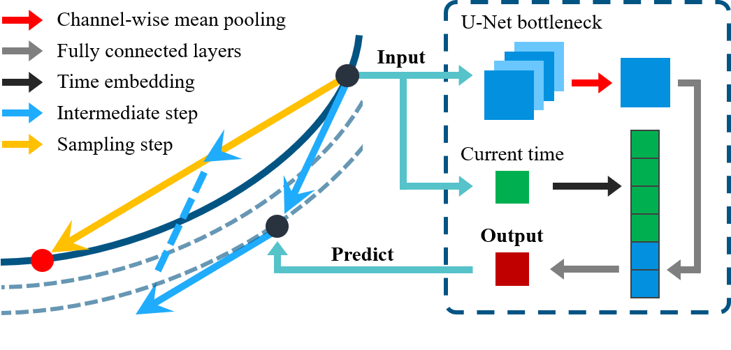
Figure 6: Network Architecture. Given the bottleneck feature extracted by the U-Net model at time $t_{n+1}$, we perform the channel-wise mean pooling and pass it through two fully connected layers. It is concatenated with the time embedding and goes through extra one fully connected layer and a sigmoid function to get the output $r$. The intermediate time step is then given by $s_{n}=t_{n}^{r}t_{n+1}^{1-r}$.

When sampling from time $t_{n+1}$ to $t_{n}$, we first perform one U-Net evaluation at $t_{n+1}$ and extract the bottleneck feature to predict and step to $s_{n}$. For AMED-Solver, another U-Net evaluation at $s_{n}$ gives the gradient term $\boldsymbol{\epsilon}_{\theta}(\mathbf{x}_{s_{n}},s_{n})$ and derives $x_{t_{n}}$ with Eq. 9. When applying AMED-Plugin on other ODE solvers, we step from $s_{n}$ to $t_{n}$ following the solver’s original sampling procedure. The total NFE is thus $2(N-1)$. We denote such a sampling process by

$$\mathbf{x}_{t_{n}}=\Phi(\mathbf{x}_{t_{n+1}},t_{n+1},t_{n},\Lambda_{n})$$ (12)

where $\Lambda_{n}$ is the set of intermediate time steps injected in $(t_{n},t_{n+1})$, $n=1,2,\cdots,N-1$.

The training of $g_{\phi}$ is based on distillation, where student and teacher sampling trajectories evaluated at $\Gamma$ are required. Denote the sampling process that generates student and teacher trajectories by $\Phi_{s}$ with $\Lambda_{n}^{s}=\{s_{n}\}$ and $\Phi_{t}$ with $\Lambda_{n}^{t}$ respectively. For $\Lambda_{n}^{t}$, since teacher trajectories require more NFE to give reliable reference, we set it to be a smooth interpolation of $M$ intermediate time steps between $t_{n}$ and $t_{n+1}$ following the original polynomial time schedule, i.e., $\Lambda_{n}^{t}=\{s_{n}^{1}\,\cdots,s_{n}^{M}\}$ where

$$s_{n}^{i}=(t_{n}^{1/\rho}+\frac{i}{M+1}(t_{n+1}^{1/\rho}-t_{n}^{1/\rho}))^{\rho}.$$ (13)

Denote the student sampling trajectory and teacher sampling trajectory extracted at $\Gamma$ by $\{\mathbf{x}_{t_{n}}\}_{n=1}^{N}$ and $\{\mathbf{y}_{t_{n}}\}_{n=1}^{N}$, we train $g_{\phi}$ using a distance metric between samples on both trajectories with $s_{n}$ predicted by $g_{\phi}$:

$$\mathcal{L}_{t_{n}}(\phi)=d(\Phi_{s}(\mathbf{x}_{t_{n+1}},t_{n+1},t_{n},\{s_{n}\}),\mathbf{y}_{t_{n}})$$ (14)

In one training loop, we first generate a batch of noise images at $t_{N}$ and then the teacher trajectories. We then calculate the loss progressively from time $t_{N-1}$ to $t_{1}$. Hence, $N-1$ backpropagations are applied in one training loop. We specify the algorithms for training and sampling in Algorithm 1 and Algorithm 2.

Consistent with the geometric property that the sampling trajectory is nearly straight when $t$ is large [6], we notice that the gradient term $\boldsymbol{\epsilon}_{\theta}(\mathbf{x}_{t_{N}},t_{N})$ at time $t_{N}$ shares almost the same direction as $x_{t_{N}}$. We thus simply use $x_{t_{N}}$ as the direction in the first sampling step to save one NFE, which is important when the budget is limited. This trick is called analytical first step (AFS) [10]. We find that the application of AFS yields little degradation or even increase of sample quality for datasets with small resolutions.

Algorithm 1 Training of $g_{\phi}$

  Input: Model parameter $\phi$, time schedule $\{t_{n}\}_{n=1}^{N}$, ODE sampler $\Phi_{s}$ and $\Phi_{t}$.

  repeat

     Sample $\mathbf{x}_{t_{N}}=\mathbf{y}_{t_{N}}\sim\mathcal{N}(\mathbf{0},t_{N}^{2}\mathbf{I})$

     Generate teacher trajectory $\{\mathbf{y}_{t_{n}}\}_{n=1}^{N}$ by $\Phi_{t}$

     for $n=N-1$ to $1$ do

        $\mathbf{x}_{t_{n}}\leftarrow\Phi_{s}(\mathbf{x}_{t_{n+1}},t_{n+1},t_{n},\{g_{\phi}(h_{t_{n+1}},t_{n+1})\})$

        # $h_{t_{n+1}}$ is extracted after U-Net evaluation at $t_{n+1}$.

        $\mathcal{L}_{t_{n}}(\phi)=d(\mathbf{x}_{t_{n}},\mathbf{y}_{t_{n}})$

        Update the model parameter $\phi$

     end for

  until convergence

Algorithm 2 AMED Sampling

  Input: Trained neural network $g_{\phi}$, time schedule $\{t_{n}\}_{n=1}^{N}$, ODE sampler $\Phi$.

  Sample $\mathbf{x}_{t_{N}}\sim\mathcal{N}(\mathbf{0},t_{N}^{2}\mathbf{I})$

  for $n=N-1$ to $1$ do

     $\mathbf{x}_{t_{n}}\leftarrow\Phi(\mathbf{x}_{t_{n+1}},t_{n+1},t_{n},\{g_{\phi}(h_{t_{n+1}},t_{n+1})\})$

  end for

  Output: Generated sample $\mathbf{x}_{t_{1}}$

3.5 Comparing with Distillation-based Methods

Though being a solver-based method, our proposed AMED-Solver shares a similar principal with distillation-based methods. The main difference is that distillation-based methods finally build a mapping from noise to data distribution by fine-tuning the pre-trained model or training a new prediction model from scratch, while our AMED-Solver still follows the nature of solving an ODE, building a flow of distributions from noise to image. Distillation-based methods have shown impressive results of performing high-quality generation by only one NFE. However, these methods require huge efforts on training. One should carefully design the training details and it takes a large amount of time to train the model (usually several or even tens of GPU days). Moreover, as distillation-based models directly build the mapping like typical generative models, they suffer from the inability of interpolating between two disconnected modes [37]. Therefore, distillation-based methods may fail in some downstream tasks requiring such an interpolation.

The training of AMED-Solver is also related to distillation, but the training goal is to properly predict the location of intermediate time steps instead of directly predicting high-dimensional samples at next time. Therefore, our architecture is very simple and is easy to train given the geometric property of sampling trajectories. The solver we obtain still maintain the nature of solving an ODE like solver-based methods, which do not suffer from obvious internal imperfection for downstream tasks.

4 Experiments

Method	NFE
	3	5	7	9
Multi-step solvers
DPM-Solver++(3M) [25]	110.0	24.97	6.74	3.42
UniPC [48]	156.3	22.32	6.46	3.47
iPNDM [22, 47]	47.98	13.59	5.08	3.17
Single-step solvers
DDIM [40]	93.36	49.66	27.93	18.43
DPM-Solver-2 [24]	155.7	57.30	10.20	4.98
EDM [18]	306.2	97.67	37.28	15.76
AMED-Solver (ours)	23.65	17.94	5.40	3.59
AMED-Plugin (ours)	17.74	7.14	3.96	2.78

(a) Unconditional generation on CIFAR10 32$\times$32. We show the results of AMED-Plugin applied on iPNDM.

Method	NFE
	3	5	7	9
Multi-step solvers
DPM-Solver++(3M) [25]	91.52	25.49	10.14	6.48
UniPC [48]	107.8	31.84	11.07	6.64
iPNDM [22, 47]	58.53	18.99	9.17	5.91
Single-step solvers
DDIM [40]	82.96	43.81	27.46	19.27
DPM-Solver-2 [24]	140.2	42.41	12.03	6.64
EDM [18]	249.4	89.63	37.65	16.76
AMED-Solver (ours)	34.70	18.51	9.13	6.56
AMED-Plugin (ours)	25.34	13.75	8.44	5.65

(b) Conditional generation on ImageNet 64$\times$64. We show the results of AMED-Plugin applied on iPNDM.

Method	NFE
	3	5	7	9
Multi-step solvers
DPM-Solver++(3M) [25]	86.45	22.51	8.44	4.77
UniPC [48]	126.4	17.89	7.07	4.53
iPNDM [22, 47]	45.98	17.17	7.79	4.58
Single-step solvers
DPM-Solver-2 [24]	266.0	87.10	22.59	9.26
AMED-Solver (ours)	44.94	15.09	7.82	5.89
AMED-Plugin (ours)	25.18	12.54	6.57	4.65

(c) Unconditional generation on FFHQ 64$\times$64. We show the results of AMED-Plugin applied on iPNDM.

Method	NFE
	3	5	7	9
Multi-step solvers
DPM-Solver++(3M) [25]	111.9	23.15	8.87	6.45
UniPC [48]	165.1	26.44	10.01	7.14
iPNDM [22, 47]	80.99	26.65	13.80	8.38
Single-step solvers
DPM-Solver-2 [24]	210.6	80.60	23.25	9.61
AMED-Solver (ours)	51.16	12.79	7.55	5.54
AMED-Plugin (ours)	113.6	24.60	8.88	6.46

(d) Unconditional generation on LSUN Bedroom 256$\times$256. We show the results of AMED-Plugin applied on DPM-Solver-2.

Table 2: Results of image generation. Our proposed AMED-Solver and AMED-Plugin achieve state-of-the-art results among solver-based methods in around 5 NFE.

4.1 Settings

Datasets. We employ AMED-Solver and AMED-Plugin on a wide range of datasets with image resolutions ranging from 32 to 512, including CIFAR10 32$\times$32 [21], FFHQ 64$\times$64 [17], ImageNet 64$\times$64 [34] and LSUN Bedroom 256$\times$256 [46]. We also give qualitative results generated by stable-diffusion [31] with resolution of 512.

Models. The pre-trained models are pixel-space models from [18] and  [43] and latent-space model from [31].

Solvers. We reimplement several representative fast ODE solvers including DDIM [40], DPM-Solver-2 [24], multi-step DPM-Solver++ [25], UniPC [48] and improved PNDM (iPNDM) [22, 47]. It is worth mentioning that we find iPNDM achieves very impressive results and outperforms other ODE solvers in many cases.

Time schedule. We mainly use the polynomial schedule with $\rho=7$, which is the default setting in [18], except for DPM-Solver++ and UniPC where we use logSNR schedule recommended in original papers [25, 48] for better results.

Training. We train $g_{\phi}$ for 20k images, which takes 5-20 minutes on CIFAR10 using a single NVIDIA A100 GPU. For datasets with resolution of 256, it takes 1-2 hours on 4 NVIDIA A100 GPUs. For the distance metric in Eq. 14, we use L2 norm in most experiments except for those on CIFAR10 where we use LPIPS for slightly better performance. For the generation of teacher trajectories for AMED-Solver, we use DPM-Solver-2 [24] or EDM [18] with doubled NFE. For AMED-Plugin, we use the same solver that generates student trajectories with $M=1$ or $2$ (we provide a detailed discussion in Sec. C.2).

Sampling. Due to designation, our AMED-Solver or AMED-Plugin naturally create solvers with even NFE. Once AFS is used, the total NFE becomes odd. With the goal of designing fast solvers in small NFE, we mainly test our method on NFE $\in\{3,5,7,9\}$ where AFS is applied. There are also results on NFE $\in\{4,6,8,10\}$ without AFS.

Evaluation. We measure the sample quality via Fréchet Inception Distance (FID) [14] with 50k samples.

4.2 Image Generation

In this section, we show the results of image generation on various datasets. For datasets with small resolution such as CIFAR10 32$\times$32, FFHQ 64$\times$64 and ImageNet 64$\times$64, we report the results of AMED-Plugin applied on iPNDM solver for its leading results. For large-resolution datasets like LSUN Bedroom, we report the results of AMED-Plugin applied on DPM-Solver-2 since the use of AFS causes inferior results for multi-step solvers in this case (see Sec. C.3 for a detailed discussion). We implement DPM-Solver++ and UniPC with order of 3, iPNDM with order of 4. To report results of DPM-Solver-2 and EDM with odd NFE, we apply AFS in their first steps.

The results are shown in Tab. 2. Our AMED-Solver exhibits promising results and outperforms other single-step methods. Besides, the AMED-Solver performs on par with multi-step solvers in datasets with small resolution, and even beats them in large-resolution cases. For the AMED-Plugin, we find it showing large boost when applied on various solvers especially for DPM-Solver-2 as shown in Tab. 2(d). Notably, the AMED-Plugin improves the FID by 6.45, 5.24 and 4.63 on CIFAR10 32$\times$32, ImageNet 64$\times$64 and FFHQ 64$\times$64 in 5 NFE. Our methods achieve state-of-the-art results in solver-based methods in around 5 NFE.

In Fig. 7, we show the learned coefficient of $g_{\phi}$ for AMED-Solver, where each $r_{n}$ is predicted by $g_{\phi}$ and $s_{n}=t_{n}^{r_{n}}t_{n+1}^{1-r_{n}}$. The dashed line recovers the default setting of DPM-Solver-2. We include more quantitative as well as qualitative results in Appendix C.

Figure 7: The learned coefficients $r_{n}$ vary in different steps and are consistently lower than the default setting.

4.3 Ablation Study

Sample-wise and Time-wise Intermediate Steps. As the U-Net bottleneck input to $g_{\phi}$ varies for different samples, the learned intermediate time steps are sample-wise, meaning that different trajectories have different time schedules. Since sampling trajectories from different starting points share similar geometric shapes, the effectiveness of inputting bottleneck might be limited. We also notice that during training, the standard deviation of learned intermediate time steps in one batch is small. Therefore, it should be safe to replace the U-Net bottleneck with zero matrix and get time-wise intermediate steps where $\{s_{n}\}_{n=1}^{N-1}$ is shared across all sampling trajectories. In Tab. 3, we provide results of sample-wise intermediate time steps learned with U-Net bottleneck as input, time-wise steps with zero matrix as input, and optimal time-wise steps obtained by a grid search of 20k samples from 0.02 to 0.98 with step size of 0.02. The results show the efficiency of AMED-Solver and again confirm the aforementioned geometric property.

Method	NFE
	4	6	8	10
Grid search (time-wise)	15.89	11.36	6.65	4.08
AMED-Solver (time-wise)	15.75	9.46	6.51	3.92
AMED-Solver (sample-wise)	15.66	9.46	5.25	3.52
Time consumption (min)
Grid search (time-wise)	69.16	88.76	113.3	142.1
AMED-Solver (time-wise)	8.60	12.73	16.87	20.93
AMED-Solver (sample-wise)	8.67	12.80	16.87	20.93

Table 3: Comparison of different strategies on CIFAR10. Grid search gives inferior results while taking more time.

Teacher solvers. In image generation, we simply let the student and teacher ODE solver to be the same, but given the property of unique encoding of ODE solvers, any ODE solver is competent to be the teacher. In Tab. 4, we use different teacher solvers for the training of $g_{\phi}$ to obtain different AMED-Solvers. It turns out that the best results are achieved when teacher solver resembles the student solver in the sampling process. We hence recommend that one should keep the teacher and student solvers to be the same.

Teacher Method	NFE
	3	5	7	9
DPM-Solver++(3M) [25]	40.43	18.55	7.04	3.88
UniPC [48]	35.06	18.02	6.52	4.01
iPNDM [22, 47]	32.09	18.12	7.20	4.24
DPM-Solver-2 [24]	25.17	17.94	6.67	3.89
EDM [18]	23.65	18.44	5.40	3.59

Table 4: Comparison of teacher methods for AMED-Solver.

Loss metric. As shown in Fig. 8, the use of LPIPS metric in the training loss Eq. 5 provides slightly better results on CIFAR10. However, applying LPIPS on datasets with large resolution or in conditional case yields worse results. We use L2 metric in these cases.

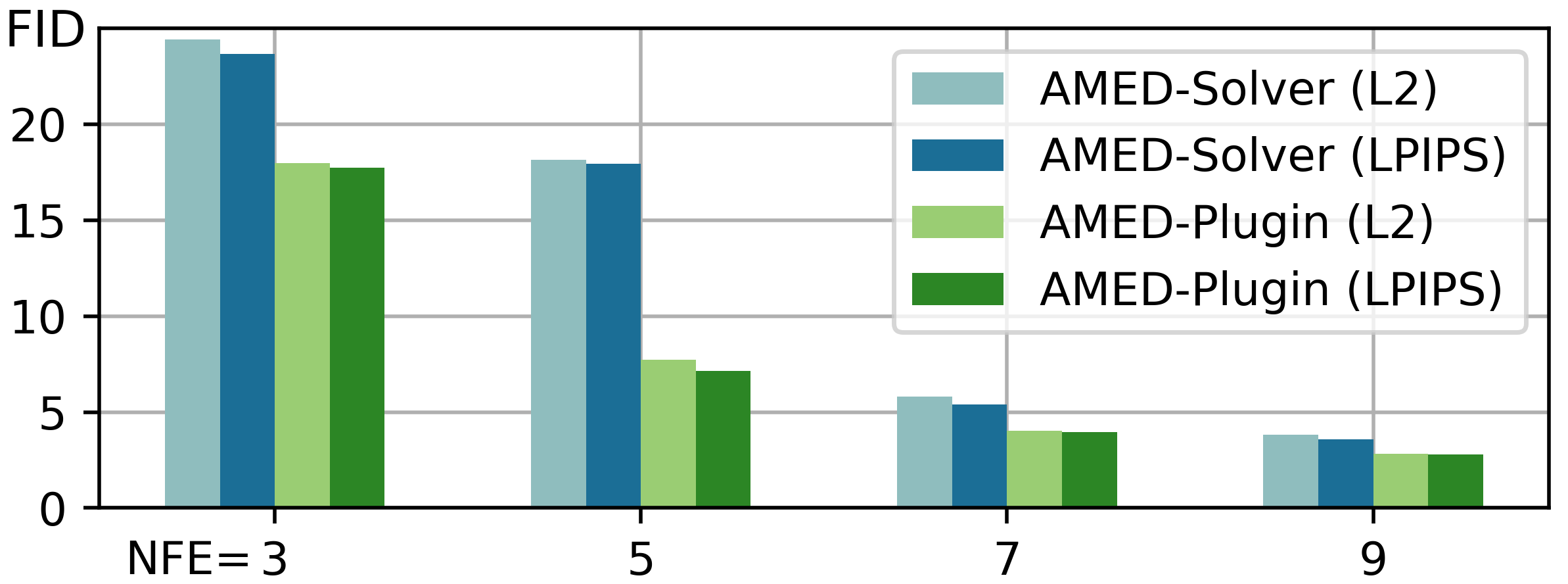
Figure 8: Ablation on loss metric on CIFAR10. We report the results of AMED-Solver and AMED-Plugin applied on iPNDM.

Time schedule. During experiments, we observe that different fast ODE solvers have different preference on time schedules. This preference even depends on the dataset. We conduct experiments on time schedules for DPM-Solver++(3M)[25] on CIFAR10 in Tab. 5 and find that it prefers logSNR schedule where the interval between the first and second time step is larger than other schedules. We also show the results of AMED-Plugin applied on these cases. The AMED-Plugin largely and consistently improves the results no matter what the time schedule is.

Time schedule	NFE
	3	5	7	9
DPM-Solver++(3M)
Uniform	76.80	26.90	16.80	13.44
Polynomial	70.04	31.66	11.30	6.45
logSNR	110.0	24.97	6.74	3.42
AMED-Plugin applied on DPM-Solver++(3M)
Uniform	40.66	17.34	13.14	10.90
Polynomial	40.24	15.54	8.18	5.24
logSNR	61.99	9.73	4.32	3.07

Table 5: FID results under different time schedules on CIFAR10. Our AMED-Plugin consistently improves the results.

5 Conclusion

In this paper, we introduce a single-step ODE solver called AMED-Solver to minimize the discretization error for fast diffusion sampling. Our key observation is that each sampling trajectory generated by existing ODE solvers approximately lies on a two-dimensional subspace, and thus the mean value theorem guarantees the learning of such a mean direction. The AMED-Solver effectively mitigates the problem of rapid sample quality degradation, which is commonly encountered in single-step methods, and shows promising results on datasets with large resolution. We also generalize the idea of AMED-Solver to AMED-Plugin, a plugin that can be applied on any fast ODE solvers to further improve the sample quality. We validate our methods through extensive experiments and achieve state-of-the-art results in extremely small NFE (around 5). We hope our attempt can inspire future works to further release the potential of fast solvers for diffusion models.

Limitation and Future Work. Fast ODE solvers for diffusion models are highly sensitive to time schedules especially when the NFE budget is limited (See Tab. 5). Through experiments, we observe that any fixed time schedule fails to perform well in all situations. In fact, our AMED-Plugin can be treated as adjusting half of the time schedule to partly alleviates but not avoids this issue. We believe that a better designation of time schedule requires further knowledge to the geometric shape of the sampling trajectory [6]. We leave this to the future work.

Supplementary Material

Appendix A Related Works

Ever since the birth of diffusion models [15, 41], their generation speed has become a major drawback compared to other generative models [12, 19]. To address this issue, efforts have been taken to accelerate the sampling of diffusion models, which fall into two main streams.

One is designing faster solvers. In early works [28, 40], the authors speed up the generation from 1000 to less than 50 NFE by reducing the number of time steps with systematic or quadratic sampling. Analytic-DPM [3], provides an analytic form of optimal variance in sampling process and improves the results. More recently, with the knowledge of interpreting the diffusion process as a PF-ODE [42], there is a class of ODE solvers based on numerical methods that accelerate the sampling process to around 10 NFE. The authors in EDM [18] achieve several improvements on training and sampling of diffusion models and propose to use Heun’s second method. PDNM [22] uses linear multi-step method to solve the PF-ODE with Runge-Kutta algorithms for the warming start. The authors in [47] recommend to use lower order linear multi-step method for warming start and propose iPNDM. Given the semi-linear structure of the PF-ODE, DPM-Solver [24] and DEIS [47] are proposed by approximate the integral involved in the analytic solution of PF-ODE with Taylor expansion and polynomial extrapolation respectively. DPM-Solver is further extend to both single-step and multi-step methods in DPM-Solver++ [25]. UniPC [48] gives a unified predictor-corrector solver and improved results compared to DPM-Solver++.

Besides training-free fast solvers above, there are also solvers requiring additional training.  [45] proposes a series of reparameterization for a generalized family of DDPM with a KID [5] loss. More related to our method, in GENIE [10], the authors apply the second truncated Taylor method [30] to the PF-ODE and distill a new model to predict the higher-order gradient term. Different from this, in AMED-Solver, we train a network that only predict the intermediate time steps, instead of a high-dimensional output.

Another mainstream is training-based distillation methods, which attempt to build a direct mapping from noise distribution to implicit data distribution. This idea is first introduced in [26] as an offline method where one needs to pre-construct a dataset generated by the original model. Rectified flow [23] also introduces an offline distillation based on optimal transport. For online distillation methods, one can progressively distill a diffusion model from more than 1k steps to 1 step  [36, 4], or utilize the consistency property of PF-ODE trajectory to tune the denoising output [8, 43, 13].

Appendix B Experimental Details

Datasets. We employ AMED-Solver and AMED-Plugin on a wide range of datasets and settings. We report results on settings including unconditional generation in both pixel and latent space, conditional generation with or without guidance. Datasets are chosen with image resolutions ranging from 32 to 512, including CIFAR10 32$\times$32 [21], FFHQ 64$\times$64 [17], ImageNet 64$\times$64 [34] and LSUN Bedroom 256$\times$256 [46]. We give qualitative results generated by stable-diffusion [31] with resolution of 512. To further evaluate the effectiveness of our methods, in Appendix C, we also include more results on LSUN Cat 256$\times$256 [46], ImageNet 256$\times$256  [34] with classifier guidance, and latent-space LSUN Bedroom 256$\times$256 [46].

Models. The pre-trained models we use throughout our experiments are pixel-space models from [18] and  [43] as well as [9], and latent-space models from [31]. Our code architecture is mainly based on the implementation in [18].

Fast ODE solvers. To give fair comparison, we reimplement several representative fast ODE solvers including DDIM [40], DPM-Solver-2 [24], multi-step DPM-Solver++ [25], UniPC [48] and improved PNDM (iPNDM) [22, 47]. Through the implementation, we obtain better or on par FID results compared with original papers. It is worth mentioning that during the implementation, we find iPNDM achieves very impressive results and outperforms other ODE solvers in many cases.

Time schedule. We notice that different ODE solvers have different preference on time schedule. We mainly use the polynomial time schedule with $\rho=7$, which is the default setting in [18], except for DPM-Solver++ and UniPC where we use logSNR time schedule recommended in original papers [25, 48] for better results. As illustrated in Sec. 3.4, the logSNR schedule is the limit case of polynomial schedule as $\rho$ approaches $+\infty$. For experiments on ImageNet with guidance, stable-diffusion and latent-space LSUN Bedroom, uniform time schedule gives best results. The reason may lie in their different training process.

Training. Since the number of parameters is small, the training of $g_{\phi}$ does not cause much computational cost. The training spends its main time on generating student and teacher trajectories. We train $g_{\phi}$ for 20k images, which takes 5-20 minutes for experiments on CIFAR10 using a single NVIDIA A100 GPU. For datasets with resolution of 256, it takes 1-2 hours on 4 NVIDIA A100 GPUs. For the distance metric in Eq. 14, we use L2 norm in most experiments except for those on CIFAR10 where we use LPIPS metric for slightly better performance. For the generation of teacher trajectories for AMED-Solver, we use DPM-Solver-2 with doubled NFE. For AMED-Plugin, we use the same solver that generates student sampling trajectories with $M=$ 1 or 2.

Sampling. Due to designation, our AMED-Solver or AMED-Plugin naturally create solvers with even NFE. Therefore once AFS is used, the total NFE become odd. With the goal of designing fast ODE solvers in extremely small NFE, we mainly test our method on NFE $\in\{3,5,7,9\}$ where AFS is applied. There are also results on NFE $\in\{4,6,8,10\}$ without using AFS.

Evaluation. We measure the sample quality via Frechet Inception Distance (FID) [14], which is a well-known quantitative evaluation metric for image quality that aligns well with human perception. For all the experiments involved, we calculate FID with 50k samples using the implementation in [18].

Appendix C Additional Results

C.1 Fast Degradation of Single-step Solvers

In pilot experiments, we find that the fast degradation of single-step solvers can be alleviated by appropriate choose of the intermediate time steps. As shown in Tab. 6, the performance of DPM-Solver-2 is very sensitive to the choice of its hyperparameter $r$. We apply AMED-Plugin to learn the appropriate $r$ and find that it achieves similar results with the best searched $r$ while adding little training overhead and negligible sampling overhead.

$r$	NFE
	4	6	8	10
0.1	28.75	17.61	11.00	5.30
0.2	24.44	21.94	8.23	4.17
0.3	37.31	30.27	6.82	3.89
0.4	75.06	43.32	7.34	4.20
0.5 (default)	146.0	60.00	10.30	5.01
0.6	241.2	79.27	15.62	6.38
AMED-Plugin	25.12	9.78	6.04	3.89

Table 6: Performance of DPM-Solver-2 on CIFAR10 is sensitive to the choice of $r$. Applying AMED-Plugin on DPM-Solver-2 efficiently help to learn the appropriate $r$.

C.2 Ablation Study on Intermediate Steps

As illustrated in Sec. 3.4, for the teacher sampling trajectory, $M$ intermediate time steps are injected in every sampling step. By using smooth interpolation, we mean that the teacher time schedule given by the original schedule $\Gamma$ combined with $\{\Gamma_{n}^{t}\}_{n=1}^{N-1}$, is equivalent to the time schedule obtained by simply setting the total number of time steps to $(M+1)(N-1)+1$ in Eq. 10 under the same $\rho$. In this way, we can easily extract samples on teacher trajectories at $\Gamma$ to get reference samples $\{\mathbf{y}_{t_{n}}\}_{n=1}^{N}$.

Here we take unconditional generation on CIFAR10 using iPNDM with AMED-Plugin as an example and provide an ablation study on the choose of $M$. The student and teacher solvers are set to be the same. The results are shown in Tab. 7. Throughout our experiments, we set $M\leq 2$.

$M$	NFE
	3	5	7	9
1	23.37	7.79	3.96	2.78
2	17.74	7.14	4.04	2.86
3	18.86	7.15	4.03	2.84
4	18.37	7.14	4.14	2.88
5	20.42	7.24	3.99	2.90

Table 7: The sensitivity of $M$ on CIFAR10 with AMED-Plugin applied on iPNDM.

C.3 Ablation Study on AFS

The trick of analytical first step (AFS) is first introduced in [10] to reduce one NFE, where the authors replace the U-Net output in the first sampling step with the direction of $x_{T}$. In Tab. 9 and Tab. 10, we provide extended results of Tab. 2(a) and Tab. 2(b) as well as the ablations between AFS and our proposed AMED-Plugin. We find that the use of AFS provides consistent improvement on datasets with resolutions of 32 and 64. The results show that in most cases they can be considered as two independent components that can together boost the performance of various ODE solvers. However, for datasets with large resolutions, applying AFS usually causes a large degradation (see Tab. 8).

Method	AFS	NFE
		3	5	7	9
DPM-Solver++(3M) [25]	2613	111.9	23.15	8.87	6.45
	1F5F8	127.5	25.04	10.51	7.32
UniPC [48]	2613	165.1	26.44	10.01	7.14
	1F5F8	103.4	21.24	17.46	6.97
iPNDM [22, 47]	2613	80.99	26.65	13.80	8.38
	1F5F8	95.61	34.61	21.96	10.06
DPM-Solver-2 [24]	2613	210.6	80.60	23.25	9.61
	1F5F8	241.8	88.79	22.59	9.07
AMED-Solver (ours)	1F5F8	51.16	12.79	7.55	5.54

Table 8: Ablation study of AFS on pixel-space LSUN Bedroom 256$\times$256.

Method	AFS	AMED	NFE
			3	4	5	6	7	8	9	10
Multi-step solvers
DPM-Solver++(3M) [25]	2613	2613	110.0	46.52	24.97	11.99	6.74	4.54	3.42	3.00
	1F5F8	2613	55.74	22.40	9.94	5.97	4.29	3.37	2.99	2.71
	2613	1F5F8	-	37.20	-	11.27	-	4.61	-	3.10
	1F5F8	1F5F8	40.83	-	10.17	-	4.45	-	3.10	-
UniPC [48]	2613	2613	156.3	41.78	22.32	12.52	6.46	4.35	3.47	3.07
	1F5F8	2613	60.74	21.97	11.36	7.06	4.73	3.56	3.10	2.72
	2613	1F5F8	-	33.36	-	11.29	-	4.83	-	3.93
	1F5F8	1F5F8	51.58	-	10.52	-	4.64	-	3.11	-
iPNDM [22, 47]	2613	2613	47.98	24.82	13.59	7.05	5.08	3.69	3.17	2.77
	1F5F8	2613	24.54	13.92	7.76	5.07	4.04	3.22	2.83	2.56
	2613	1F5F8	-	15.06	-	6.63	-	3.94	-	2.84
	1F5F8	1F5F8	17.74	-	7.14	-	3.96	-	2.79	-
Single-step solvers
DDIM [40]	2613	2613	93.36	66.76	49.66	35.62	27.93	22.32	18.43	15.69
	1F5F8	2613	67.26	49.96	35.78	28.00	22.37	18.48	15.69	13.47
	2613	1F5F8	-	47.48	-	31.62	-	21.69	-	15.26
	1F5F8	1F5F8	50.64	-	31.74	-	21.80	-	15.27	-
DPM-Solver-2 [24]	2613	2613	-	146.0	-	60.00	-	10.30	-	5.01
	1F5F8	2613	155.7	-	57.28	-	10.20	-	4.98	-
	2613	1F5F8	-	25.12	-	21.40	-	6.04	-	3.89
	1F5F8	1F5F8	43.51	-	23.04	-	6.79	-	4.26	-
AMED-Solver (ours)	2613	1F5F8	-	15.66	-	9.46	-	5.25	-	3.52
	1F5F8	1F5F8	23.65	-	17.94	-	5.40	-	3.59	-

Table 9: Unconditional generation on CIFAR10 32$\times$32.

Method	AFS	AMED	NFE
			3	4	5	6	7	8	9	10
Multi-step solvers
DPM-Solver++(3M) [25]	2613	2613	91.52	56.34	25.49	15.06	10.14	7.84	6.48	5.67
	1F5F8	2613	65.20	30.56	16.87	11.38	8.68	7.12	6.25	5.58
	2613	1F5F8	-	66.52	-	14.68	-	8.19	-	6.04
	1F5F8	1F5F8	71.12	-	18.13	-	8.98	-	5.98	-
UniPC [48]	2613	2613	107.8	68.16	31.84	17.37	11.07	8.25	6.64	5.59
	1F5F8	2613	75.21	37.74	18.62	12.07	8.77	6.83	5.73	4.98
	2613	1F5F8	-	55.84	-	16.22	-	9.03	-	6.38
	1F5F8	1F5F8	70.57	-	16.82	-	9.07	-	5.61	-
iPNDM [22, 47]	2613	2613	58.53	33.79	18.99	12.92	9.17	7.20	5.91	5.11
	1F5F8	2613	34.81	21.32	15.53	10.27	8.64	6.60	5.64	4.97
	2613	1F5F8	-	23.12	-	11.95	-	7.01	-	5.11
	1F5F8	1F5F8	25.34	-	13.75	-	8.44	-	5.64	-
Single-step solvers
DDIM [40]	2613	2613	82.96	58.43	43.81	34.03	27.46	22.59	19.27	16.72
	1F5F8	2613	62.42	46.06	35.48	28.50	23.31	19.82	17.14	15.02
	2613	1F5F8	-	41.80	-	32.49	-	22.04	-	16.60
	1F5F8	1F5F8	48.72	-	33.42	-	23.06	-	16.94	-
DPM-Solver-2 [24]	2613	2613	-	129.8	-	44.83	-	12.42	-	6.84
	1F5F8	2613	140.2	-	42.41	-	12.03	-	6.64	-
	2613	1F5F8	-	41.90	-	29.74	-	11.47	-	6.98
	1F5F8	1F5F8	76.26	-	29.75	-	11.48	-	6.81	-
AMED-Solver (ours)	2613	1F5F8	-	30.03	-	19.24	-	9.58	-	6.60
	1F5F8	1F5F8	34.70	-	18.51	-	9.13	-	6.56	-

Table 10: Conditional generation on ImageNet 64$\times$64.

C.4 More Quantitative Results

In this section, we provide additional quantitative results on more datasets including LSUN Cat 256$\times$256 [46], latent-space LSUN Bedroom 256$\times$256 [46, 31] and ImageNet 256$\times$256 [34] with classifier guidance [9]. The results are shown in Tab. 11, Tab. 12 and Tab. 13.

Method	NFE
	3	5	7	9
DPM-Solver++(3M) [25]	114.5	42.80	22.71	17.26
UniPC [48]	140.2	41.73	23.31	17.69
iPNDM [22, 47]	69.68	30.52	16.69	10.48
DPM-Solver-2 [24]	205.4	60.99	23.72	12.81
AMED-Solver (ours)	71.13	27.30	16.00	11.46

Table 11: Unconditional generation on LSUN Cat.

Method	NFE
	3	5	7	9
DPM-Solver++(3M) [25]	115.7	18.44	5.18	3.76
AMED-Plugin (ours)	61.93	9.00	4.38	3.62

Table 12: Unconditional generation on latent-space LSUN Bedroom. AMED-Plugin is applied on DPM-Solver++.

Method	NFE
	4	6	8	10
Guidance scale = 8.0
DPM-Solver++(3M) [25]	60.01	25.51	11.98	7.95
AMED-Plugin (ours)	53.74	19.29	12.63	8.95
Guidance scale = 4.0
DPM-Solver++(3M) [25]	27.15	10.25	7.10	6.15
AMED-Plugin (ours)	31.73	8.87	6.90	5.99
Guidance scale = 2.0
DPM-Solver++(3M) [25]	23.06	10.17	7.04	5.92
AMED-Plugin (ours)	34.87	10.14	6.68	5.70

Table 13: Conditional generation on ImageNet256 with classifier guidance. AMED-Plugin is applied on DPM-Solver++.

C.5 More Qualitative Results

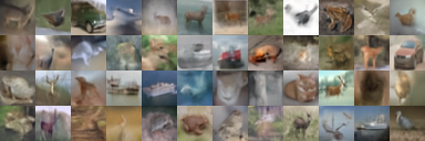
(a) Baseline iPNDM solver. FID = 47.98.

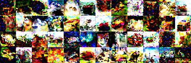
(b) Baseline DPM-Solver-2. FID = 155.7.

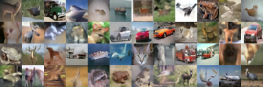
(c) AMED-Plugin applied on iPNDM solver. FID = 17.74.

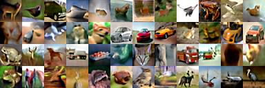
(d) AMED-Solver. FID = 23.65.

Figure 11: Uncurated samples on CIFAR10 32$\times$32 with 3 NFE.

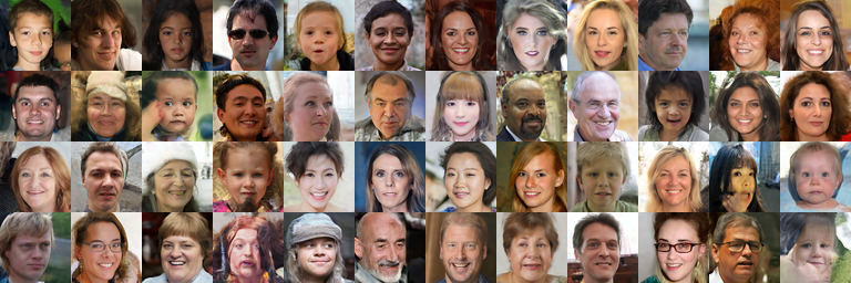
(a) Baseline iPNDM solver. FID = 17.17.

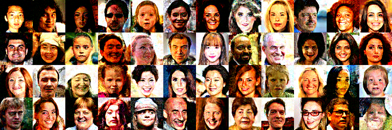
(b) Baseline DPM-Solver-2. FID = 87.10.

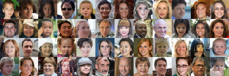
(c) AMED-Plugin applied on iPNDM solver. FID = 12.54.

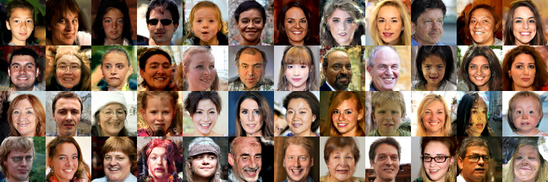
(d) AMED-Solver. FID = 15.09.

Figure 16: Uncurated samples on FFHQ 64$\times$64 with 5 NFE.

We give more qualitative results generated by stable-diffusion-v1 [31] with a default classifier-free guidance scale 7.5 in Fig. 9. Results on various datasets with NFE of 3 and 5 are provided from Fig. 11 to Fig. 16.

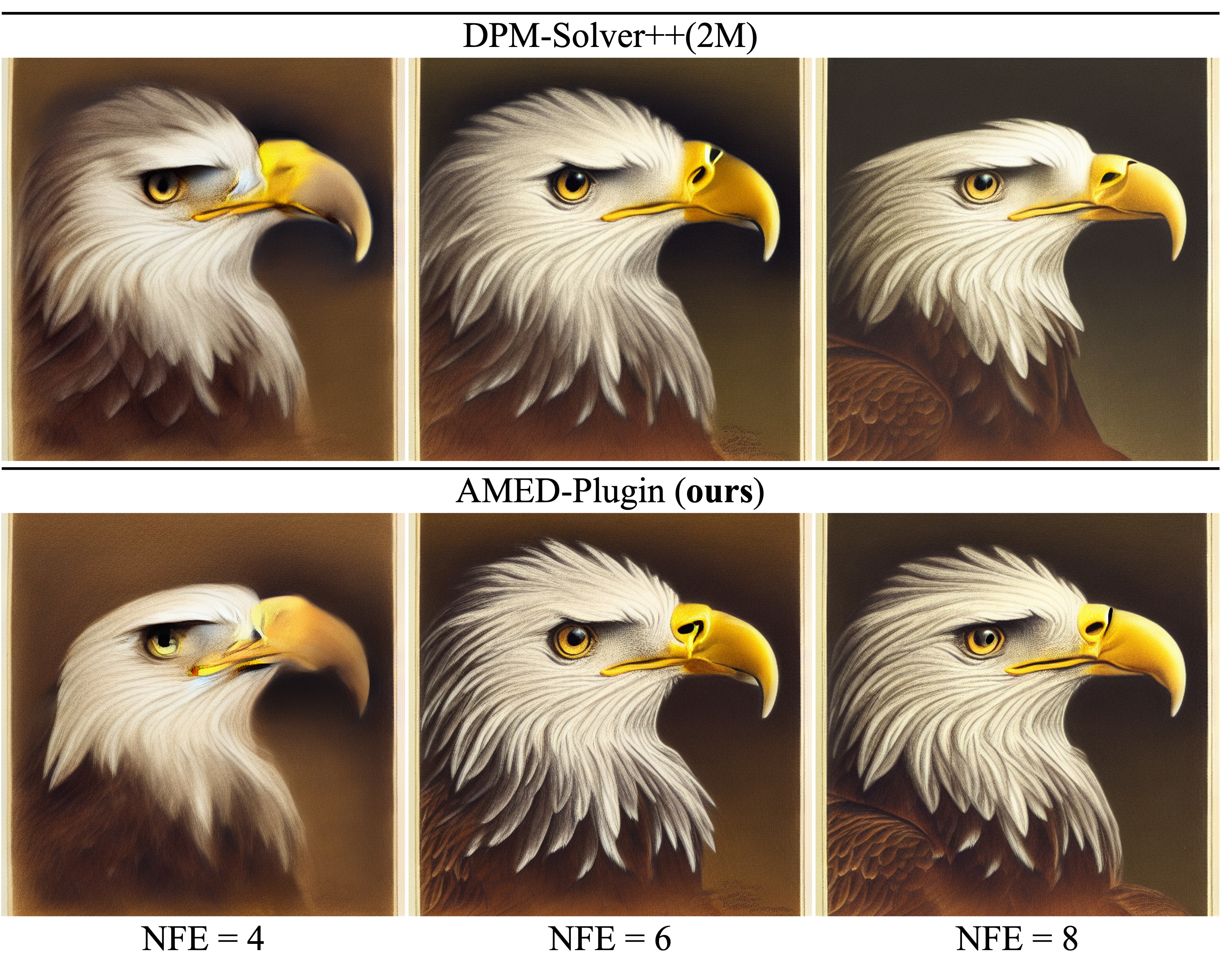
(a) Text prompt: ”A portrait of an eagle”.

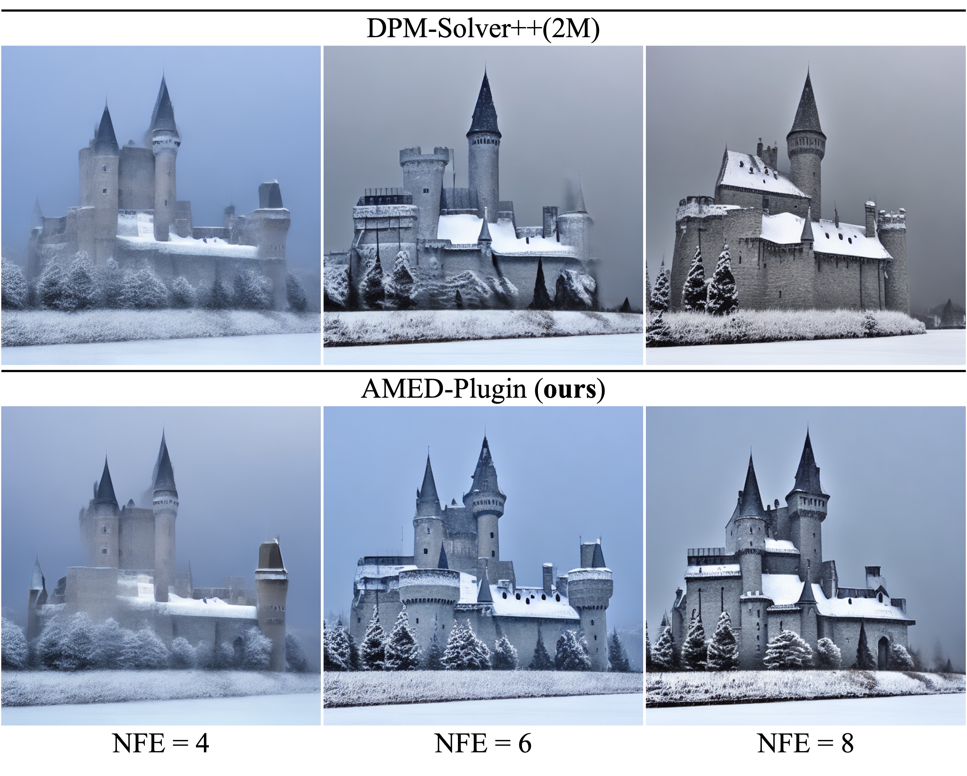
(b) Text prompt: ”Under a gray sky, a castle in ice and snow”.

Figure 9: Synthesized images by Stable-Diffusion-v1 [31] with default classifier-free guidance scale 7.5.

Appendix D Theoretical Analysis

In Sec. 3.1, we experimentally showed that the sampling trajectory of diffusion models generated by an ODE solver almost lies in a two-dimensional subspace embedded in the ambient space. This is the core condition for the mean value theorem to approximately hold in the vector-valued function case. However, the sampling trajectory would not necessarily lie in a plane. In this section, we analyze to what extent will this affects our AMED-Solver, where we set the two-dimensional subspace to be the place spanned by the first two principal components.

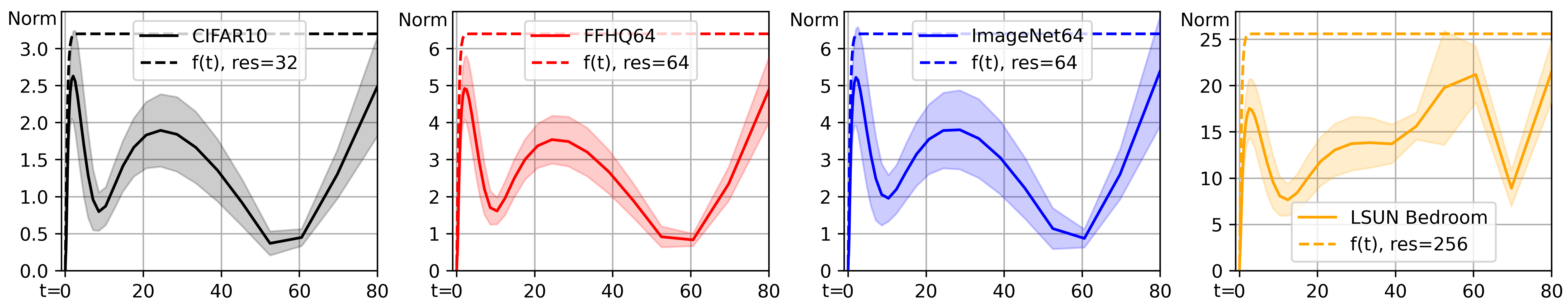
Figure 10: Following the experiment in Sec. 3.1, we calculate $\left\|\mathbf{x}_{t}-\tilde{\mathbf{x}}_{t}\right\|_{2}$ and find that we can bound it by a proper setting of Eq. 16.

Notations. Denote $d$ as the dimension of the ambient space. Let $\{\mathbf{x}_{\tau}\}_{\tau=\epsilon}^{T}$ to be the solution of the PF-ODE Eq. 6. Let $\{\tilde{\mathbf{x}}_{\tau}\}_{\tau=\epsilon}^{T}$ to be the trajectory obtained by projecting $\{\mathbf{x}_{\tau}\}_{\tau=\epsilon}^{T}$ to the two-dimensional subspace spanned by its first two principal components. Given $\epsilon\leq s<m<t\leq T$, one step of the AMED-Solver is given by

$$\mathbf{x}_{s}^{A}=\mathbf{x}_{t}+(s-t)\boldsymbol{\epsilon}_{\theta}(\mathbf{x}_{m},m).$$ (15)

Define the scaled logistic function to be

$$f(\tau)=a\left(\frac{1}{1+e^{-b\tau}}-\frac{1}{2}\right),\tau\in\mathbb{R};a,b\in\mathbb{R}^{+}.$$ (16)

Finally, define a SDE

$$\mathrm{d}\mathbf{z}_{\tau}=g(\tau)\mathrm{d}\mathbf{w}_{\tau},\tau\in[s,t]$$ (17)

with initial value $\bf 0$ at $t$ where $g(\tau)$ is a real-valued function and $\mathbf{w}_{\tau}\in\mathbb{R}^{d}$ is the standard Wiener process.

We start by the following assumptions:

Assumption 1.

Assume that there exists $a,b>0$ s.t. $\left\|\mathbf{x}_{\tau}-\tilde{\mathbf{x}}_{\tau}\right\|_{2}\leq f(\tau),\tau\in[\epsilon,T]$.

For the choice of $a$ and $b$, in Fig. 10, we calculate $\left\|\mathbf{x}_{\tau}-\tilde{\mathbf{x}}_{\tau}\right\|_{2}$ following the experiment settings in Sec. 3.1. We experimentally find that $\left\|\mathbf{x}_{\tau}-\tilde{\mathbf{x}}_{\tau}\right\|_{2}$ can be roughly upper bounded by setting $a=\sqrt{3d}/15$ and $b=3$.

Assumption 2.

Assume that there exists an integrable function $\boldsymbol{\omega}:\mathbb{R}^{d+1}\to\mathbb{R}^{d}$ that generate $\{\tilde{\mathbf{x}}_{\tau}\}_{\tau=\epsilon}^{T}$ by

$$\tilde{\mathbf{x}}_{s}=\tilde{\mathbf{x}}_{t}+\int_{t}^{s}\boldsymbol{\epsilon}_{\theta}(\mathbf{x}_{\tau},\tau)+\boldsymbol{\omega}(\mathbf{x}_{\tau},\tau)\mathrm{d}\tau.$$ (18)

with initial value $\tilde{\mathbf{x}}_{T}$. In this way, we can decompose the integral in Eq. 7 into two components that parallel and perpendicular to the plane where $\{\tilde{\mathbf{x}}_{\tau}\}_{\tau=\epsilon}^{T}$ lies, i.e.,

$$\int_{t}^{s}\boldsymbol{\epsilon}_{\theta}(\mathbf{x}_{\tau},\tau)\mathrm{d}\tau= \int_{t}^{s}\boldsymbol{\epsilon}_{\theta}(\mathbf{x}_{\tau},\tau)\boldsymbol{\omega}(\mathbf{x}_{\tau},\tau)\mathrm{d}\tau$$ (19)

$$-\int_{t}^{s}\boldsymbol{\omega}(\mathbf{x}_{\tau},\tau)\mathrm{d}\tau.$$

Assumption 3.

Decompose $\boldsymbol{\epsilon}_{\theta}(\mathbf{x}_{m},m)$ in Eq. 15 into two components as in Assumption 2 that parallel and perpendicular to the plane where $\{\tilde{\mathbf{x}}_{\tau}\}_{\tau=\epsilon}^{T}$ lies:

$$\boldsymbol{\epsilon}_{\theta}(\mathbf{x}_{m},m)=\boldsymbol{\epsilon}_{\theta}^{\parallel}(\mathbf{x}_{m},m)+\boldsymbol{\epsilon}_{\theta}^{\perp}(\mathbf{x}_{m},m).$$ (20)

Assume that the parallel component is optimally learned and for the perpendicular component, we have

$$\left\|(s-t)\boldsymbol{\epsilon}_{\theta}^{\perp}(\mathbf{x}_{m},m)\right\|_{2}\leq\left\|\int_{t}^{s}\boldsymbol{\omega}(\mathbf{x}_{\tau},\tau)\mathrm{d}\tau\right\|_{2}.$$ (21)

Assumption 4.

There exists such a $g(\tau)$ s.t. with high probability that

$$\left\|\int_{t}^{s}\boldsymbol{\omega}(\tilde{\mathbf{x}}_{\tau},\tau)\mathrm{d}\tau\right\|_{2}\leq\left\|\mathbf{z}_{s}\right\|_{2}.$$ (22)

Lemma 1.

Under assumption 1 and 4, let $g(\tau)=f(\tau)/\sqrt{d}$, then $\mathbf{z}_{s}$ concentrates at a thin shell with radius

$$r(s,t)=\frac{a}{\sqrt{b}}\sqrt{\frac{1}{1+e^{x}}\bigg{|}_{bs}^{bt}+\frac{b}{4}(t-s)}.$$ (23)

Proof.

Since the SDE Eq. 17 has zero drift coefficient, its perturbation kernel $p(\mathbf{z}_{s}|\mathbf{z}_{t}=\bf 0)$ is a Gaussian with zero mean [38]. The covariance $\mathbf{P}(s,t)$ is given by

$$\mathbf{P}(s,t) =\int_{s}^{t}g^{2}(\tau)\mathrm{d}\tau\mathbf{I}$$ (24)

$$=\frac{a^{2}}{d}\int_{s}^{t}\left(\frac{1}{1+e^{-b\tau}}-\frac{1}{2}\right)^{2}\mathrm{d}\tau\mathbf{I}$$ (25)

$$=\underbrace{\frac{a^{2}}{bd}\left(\frac{1}{1+e^{x}}\bigg{|}_{bs}^{bt}+\frac{b}{4}(t-s)\right)}_{{\sigma^{2}(s,t)}}\mathbf{I}.$$ (26)

By the well-known concentration of measure [44], there exists a constant $c>0$ s.t. for any $h\geq 0$, we have

$$\mathbb{P}\left(\left|\left\|\mathbf{z}_{s}\right\|_{2}-\left|\sigma(s,t)\right|\sqrt{d}\right|\geq h\right)\leq 2e^{-ch^{2}}$$ (27)

which complete the proof. ∎

Proposition 1.

Given $\epsilon\leq s<t\leq T$, under the assumptions and Lemma 1 above, with high probability we have

$$\left\|\mathbf{x}_{s}-\mathbf{x}_{s}^{A}\right\|_{2}\leq f(s)+f(t)+r(s,t).$$ (28)

Proof.

Under assumptions and Lemma 1 above, we have

$$\left\|\mathbf{x}_{s}-\mathbf{x}_{s}^{A}\right\|_{2}$$ (29)

$$\leq\left\|\mathbf{x}_{s}-\tilde{\mathbf{x}}_{s}\right\|_{2}+\left\|\tilde{\mathbf{x}}_{s}-\mathbf{x}_{s}^{A}\right\|_{2}$$ (30)

$$\leq f(s)+\Bigl{|}\Bigl{|}\mathbf{x}_{t}-\tilde{\mathbf{x}}_{t}+(s-t)\boldsymbol{\epsilon}_{\theta}(\mathbf{x}_{m},m)$$ (31)

$$\quad-\int_{t}^{s}\boldsymbol{\epsilon}_{\theta}(\mathbf{x}_{\tau},\tau)+\boldsymbol{\omega}(\mathbf{x}_{\tau},\tau)\mathrm{d}\tau\Bigl{|}\Bigl{|}_{2}$$ (32)

$$\leq f(s)+f(t)+\Bigl{|}\Bigl{|}(s-t)\boldsymbol{\epsilon}_{\theta}^{\perp}(\mathbf{x}_{m},m)$$ (33)

$$\quad+(s-t)\boldsymbol{\epsilon}_{\theta}^{\parallel}(\mathbf{x}_{m},m)-\int_{t}^{s}(\boldsymbol{\epsilon}_{\theta}+\boldsymbol{\omega})(\mathbf{x}_{\tau},\tau)\mathrm{d}\tau\Bigl{|}\Bigl{|}_{2}$$ (34)

$$\leq f(s)+f(t)+\left\|(s-t)\boldsymbol{\epsilon}_{\theta}^{\perp}(\mathbf{x}_{m},m)\right\|_{2}$$ (35)

$$\leq f(s)+f(t)+\left\|\int_{t}^{s}\boldsymbol{\omega}(\mathbf{x}_{\tau},\tau)\mathrm{d}\tau\right\|_{2}$$ (36)

$$\leq f(s)+f(t)+r(s,t)$$ (37)

with high probability. ∎

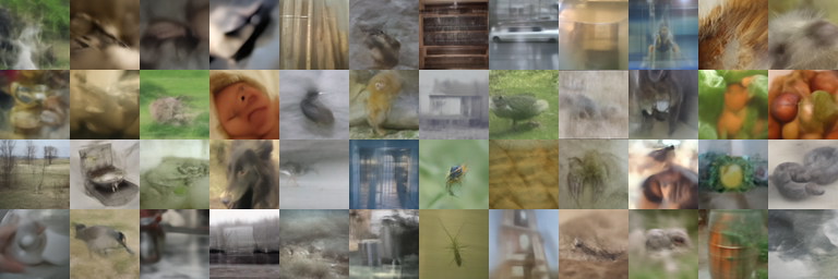
(a) Baseline iPNDM solver. FID = 58.53.

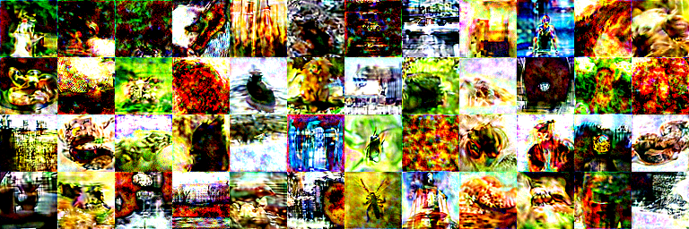
(b) Baseline DPM-Solver-2. FID = 140.2.

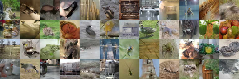
(c) AMED-Plugin applied on iPNDM solver. FID = 25.34.

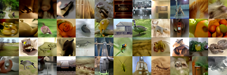
(d) AMED-Solver. FID = 34.70.

Figure 12: Uncurated samples on Imagenet 64$\times$64 with 3 NFE.

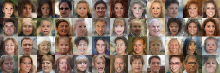
(a) Baseline iPNDM solver. FID = 45.98.

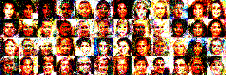
(b) Baseline DPM-Solver-2. FID = 266.0.

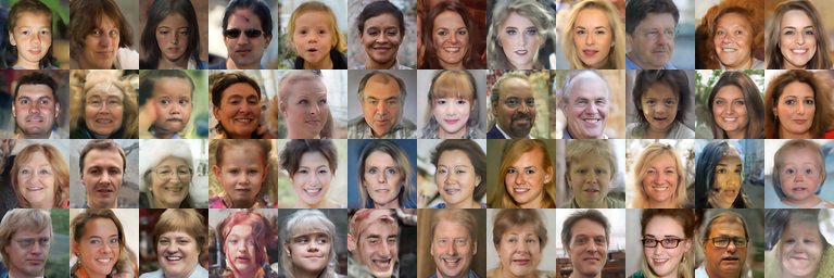
(c) AMED-Plugin applied on iPNDM solver. FID = 25.18.

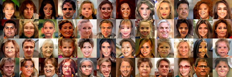
(d) AMED-Solver. FID = 44.94.

Figure 13: Uncurated samples on FFHQ 64$\times$64 with 3 NFE.

(a) Baseline iPNDM solver. FID = 13.59.

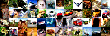
(b) Baseline DPM-Solver-2. FID = 57.30.

(c) AMED-Plugin applied on iPNDM solver. FID = 7.14.

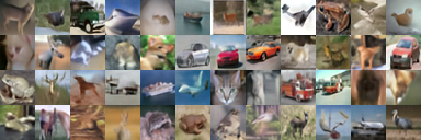
(d) AMED-Solver. FID = 17.94.

Figure 14: Uncurated samples on CIFAR10 32$\times$32 with 5 NFE.

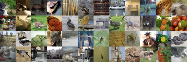
(a) Baseline iPNDM solver. FID = 18.99.

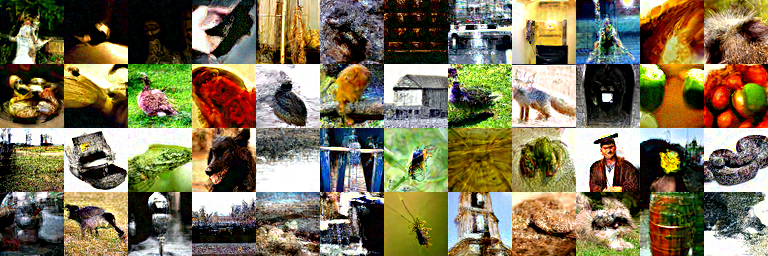
(b) Baseline DPM-Solver-2. FID = 42.41.

(c) AMED-Plugin applied on iPNDM solver. FID = 13.75.

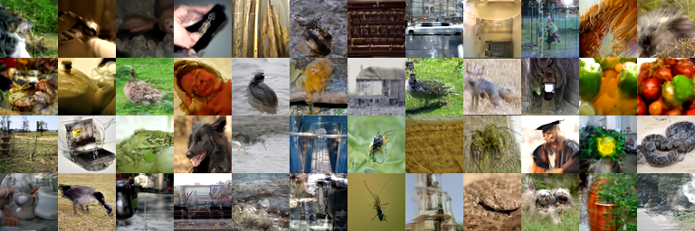
(d) AMED-Solver. FID = 18.51.

Figure 15: Uncurated samples on Imagenet 64$\times$64 with 5 NFE.

References

- Anderson [1982] Brian DO Anderson. Reverse-time diffusion equation models. Stochastic Processes and their Applications, 12(3):313–326, 1982.
- Atkinson et al. [2011] Kendall Atkinson, Weimin Han, and David E Stewart. Numerical solution of ordinary differential equations. John Wiley & Sons, 2011.
- Bao et al. [2022] Fan Bao, Chongxuan Li, Jun Zhu, and Bo Zhang. Analytic-dpm: an analytic estimate of the optimal reverse variance in diffusion probabilistic models. arXiv preprint arXiv:2201.06503, 2022.
- Berthelot et al. [2023] David Berthelot, Arnaud Autef, Jierui Lin, Dian Ang Yap, Shuangfei Zhai, Siyuan Hu, Daniel Zheng, Walter Talbot, and Eric Gu. Tract: Denoising diffusion models with transitive closure time-distillation. arXiv preprint arXiv:2303.04248, 2023.
- Bińkowski et al. [2018] Mikołaj Bińkowski, Danica J Sutherland, Michael Arbel, and Arthur Gretton. Demystifying mmd gans. arXiv preprint arXiv:1801.01401, 2018.
- Chen et al. [2023] Defang Chen, Zhenyu Zhou, Jian-Ping Mei, Chunhua Shen, Chun Chen, and Can Wang. A geometric perspective on diffusion models. arXiv preprint arXiv:2305.19947, 2023.
- Cheney et al. [2001] Elliott Ward Cheney, EW Cheney, and W Cheney. Analysis for applied mathematics. Springer, 2001.
- Daras et al. [2023] Giannis Daras, Yuval Dagan, Alexandros G Dimakis, and Constantinos Daskalakis. Consistent diffusion models: Mitigating sampling drift by learning to be consistent. arXiv preprint arXiv:2302.09057, 2023.
- Dhariwal and Nichol [2021] Prafulla Dhariwal and Alex Nichol. Diffusion models beat gans on image synthesis. In Advances in Neural Information Processing Systems, 2021.
- Dockhorn et al. [2022] Tim Dockhorn, Arash Vahdat, and Karsten Kreis. Genie: Higher-order denoising diffusion solvers. In Advances in Neural Information Processing Systems, 2022.
- Feller [1949] William Feller. On the theory of stochastic processes, with particular reference to applications. In Proceedings of the First Berkeley Symposium on Mathematical Statistics and Probability, pages 403–432, 1949.
- Goodfellow et al. [2014] Ian Goodfellow, Jean Pouget-Abadie, Mehdi Mirza, Bing Xu, David Warde-Farley, Sherjil Ozair, Aaron Courville, and Yoshua Bengio. Generative adversarial nets. Advances in neural information processing systems, 27, 2014.
- Gu et al. [2023] Jiatao Gu, Shuangfei Zhai, Yizhe Zhang, Lingjie Liu, and Joshua M Susskind. Boot: Data-free distillation of denoising diffusion models with bootstrapping. In ICML 2023 Workshop on Structured Probabilistic Inference & Generative Modeling, 2023.
- Heusel et al. [2017] Martin Heusel, Hubert Ramsauer, Thomas Unterthiner, Bernhard Nessler, and Sepp Hochreiter. GANs trained by a two time-scale update rule converge to a local Nash equilibrium. In Advances in Neural Information Processing Systems, pages 6626–6637, 2017.
- Ho et al. [2020] Jonathan Ho, Ajay Jain, and Pieter Abbeel. Denoising diffusion probabilistic models. In Advances in Neural Information Processing Systems, 2020.
- Hyvärinen [2005] Aapo Hyvärinen. Estimation of non-normalized statistical models by score matching. Journal of Machine Learning Research, 6:695–709, 2005.
- Karras et al. [2019] Tero Karras, Samuli Laine, and Timo Aila. A style-based generator architecture for generative adversarial networks. In Proceedings of the IEEE/CVF conference on computer vision and pattern recognition, pages 4401–4410, 2019.
- Karras et al. [2022] Tero Karras, Miika Aittala, Timo Aila, and Samuli Laine. Elucidating the design space of diffusion-based generative models. In Advances in Neural Information Processing Systems, 2022.
- Kingma and Welling [2013] Diederik P Kingma and Max Welling. Auto-encoding variational bayes. arXiv preprint arXiv:1312.6114, 2013.
- Kingma et al. [2021] Diederik P Kingma, Tim Salimans, Ben Poole, and Jonathan Ho. Variational diffusion models. In Advances in Neural Information Processing Systems, 2021.
- Krizhevsky and Hinton [2009] Alex Krizhevsky and Geoffrey Hinton. Learning multiple layers of features from tiny images. Technical Report, 2009.
- Liu et al. [2022a] Luping Liu, Yi Ren, Zhijie Lin, and Zhou Zhao. Pseudo numerical methods for diffusion models on manifolds. In International Conference on Learning Representations, 2022a.
- Liu et al. [2022b] Xingchao Liu, Chengyue Gong, and Qiang Liu. Flow straight and fast: Learning to generate and transfer data with rectified flow. arXiv preprint arXiv:2209.03003, 2022b.
- Lu et al. [2022a] Cheng Lu, Yuhao Zhou, Fan Bao, Jianfei Chen, Chongxuan Li, and Jun Zhu. Dpm-solver: A fast ode solver for diffusion probabilistic model sampling in around 10 steps. In Advances in Neural Information Processing Systems, 2022a.
- Lu et al. [2022b] Cheng Lu, Yuhao Zhou, Fan Bao, Jianfei Chen, Chongxuan Li, and Jun Zhu. Dpm-solver++: Fast solver for guided sampling of diffusion probabilistic models. arXiv preprint arXiv:2211.01095, 2022b.
- Luhman and Luhman [2021] Eric Luhman and Troy Luhman. Knowledge distillation in iterative generative models for improved sampling speed. arXiv preprint arXiv:2101.02388, 2021.
- Maoutsa et al. [2020] Dimitra Maoutsa, Sebastian Reich, and Manfred Opper. Interacting particle solutions of fokker–planck equations through gradient–log–density estimation. arXiv preprint arXiv:2006.00702, 2020.
- Nichol and Dhariwal [2021] Alexander Quinn Nichol and Prafulla Dhariwal. Improved denoising diffusion probabilistic models. In International Conference on Machine Learning, pages 8162–8171. PMLR, 2021.
- Oksendal [2013] Bernt Oksendal. Stochastic differential equations: an introduction with applications. Springer Science & Business Media, 2013.
- Platen and Bruti-Liberati [2010] Eckhard Platen and Nicola Bruti-Liberati. Numerical solution of stochastic differential equations with jumps in finance. Springer Science & Business Media, 2010.
- Rombach et al. [2022] Robin Rombach, Andreas Blattmann, Dominik Lorenz, Patrick Esser, and Björn Ommer. High-resolution image synthesis with latent diffusion models. In Proceedings of the IEEE/CVF Conference on Computer Vision and Pattern Recognition, pages 10684–10695, 2022.
- Ronneberger et al. [2015] Olaf Ronneberger, Philipp Fischer, and Thomas Brox. U-net: Convolutional networks for biomedical image segmentation. In Medical Image Computing and Computer-Assisted Intervention–MICCAI 2015: 18th International Conference, Munich, Germany, October 5-9, 2015, Proceedings, Part III 18, pages 234–241. Springer, 2015.
- Ruiz et al. [2023] Nataniel Ruiz, Yuanzhen Li, Varun Jampani, Yael Pritch, Michael Rubinstein, and Kfir Aberman. Dreambooth: Fine tuning text-to-image diffusion models for subject-driven generation. In Proceedings of the IEEE/CVF Conference on Computer Vision and Pattern Recognition, pages 22500–22510, 2023.
- Russakovsky et al. [2015] Olga Russakovsky, Jia Deng, Hao Su, Jonathan Krause, Sanjeev Satheesh, Sean Ma, Zhiheng Huang, Andrej Karpathy, Aditya Khosla, Michael S. Bernstein, Alexander C. Berg, and Fei-Fei Li. Imagenet large scale visual recognition challenge. International Journal of Computer Vision, 115(3):211–252, 2015.
- Saharia et al. [2022] Chitwan Saharia, William Chan, Saurabh Saxena, Lala Li, Jay Whang, Emily L Denton, Kamyar Ghasemipour, Raphael Gontijo Lopes, Burcu Karagol Ayan, Tim Salimans, et al. Photorealistic text-to-image diffusion models with deep language understanding. In Advances in Neural Information Processing Systems, pages 36479–36494, 2022.
- Salimans and Ho [2022] Tim Salimans and Jonathan Ho. Progressive distillation for fast sampling of diffusion models. In International Conference on Learning Representations, 2022.
- Salmona et al. [2022] Antoine Salmona, Valentin De Bortoli, Julie Delon, and Agnès Desolneux. Can push-forward generative models fit multimodal distributions? Advances in Neural Information Processing Systems, 35:10766–10779, 2022.
- Särkkä and Solin [2019] Simo Särkkä and Arno Solin. Applied stochastic differential equations. Cambridge University Press, 2019.
- Sohl-Dickstein et al. [2015] Jascha Sohl-Dickstein, Eric Weiss, Niru Maheswaranathan, and Surya Ganguli. Deep unsupervised learning using nonequilibrium thermodynamics. In International conference on machine learning, pages 2256–2265. PMLR, 2015.
- Song et al. [2021a] Jiaming Song, Chenlin Meng, and Stefano Ermon. Denoising diffusion implicit models. In International Conference on Learning Representations, 2021a.
- Song and Ermon [2019] Yang Song and Stefano Ermon. Generative modeling by estimating gradients of the data distribution. In Advances in Neural Information Processing Systems, 2019.
- Song et al. [2021b] Yang Song, Jascha Sohl-Dickstein, Diederik P. Kingma, Abhishek Kumar, Stefano Ermon, and Ben Poole. Score-based generative modeling through stochastic differential equations. In International Conference on Learning Representations, 2021b.
- Song et al. [2023] Yang Song, Prafulla Dhariwal, Mark Chen, and Ilya Sutskever. Consistency models. In International Conference on Machine learning, 2023.
- Vershynin [2018] Roman Vershynin. High-dimensional probability: An introduction with applications in data science. Cambridge university press, 2018.
- Watson et al. [2021] Daniel Watson, William Chan, Jonathan Ho, and Mohammad Norouzi. Learning fast samplers for diffusion models by differentiating through sample quality. In International Conference on Learning Representations, 2021.
- Yu et al. [2015] Fisher Yu, Ari Seff, Yinda Zhang, Shuran Song, Thomas Funkhouser, and Jianxiong Xiao. Lsun: Construction of a large-scale image dataset using deep learning with humans in the loop. arXiv preprint arXiv:1506.03365, 2015.
- Zhang and Chen [2023] Qinsheng Zhang and Yongxin Chen. Fast sampling of diffusion models with exponential integrator. In International Conference on Learning Representations, 2023.
- Zhao et al. [2023] Wenliang Zhao, Lujia Bai, Yongming Rao, Jie Zhou, and Jiwen Lu. Unipc: A unified predictor-corrector framework for fast sampling of diffusion models. arXiv preprint arXiv:2302.04867, 2023.