Mixture of Gaussian-distributed Prototypes with Generative Modelling
for Interpretable Image Classification

Abstract

Prototypical-part interpretable methods, e.g., ProtoPNet, enhance interpretability by connecting classification predictions to class-specific training prototypes, thereby offering an intuitive insight into their decision-making. Current methods rely on a discriminative classifier trained with point-based learning techniques that provide specific values for prototypes. Such prototypes have relatively low representation power due to their sparsity and potential redundancy, with each prototype containing no variability measure. In this paper, we present a new generative learning of prototype distributions, named Mixture of Gaussian-distributed Prototypes (MGProto), which are represented by Gaussian mixture models (GMM). Such an approach enables the learning of more powerful prototype representations since each learned prototype will own a measure of variability, which naturally reduces the sparsity given the spread of the distribution around each prototype, and we also integrate a prototype diversity objective function into the GMM optimisation to reduce redundancy. Incidentally, the generative nature of MGProto offers a new and effective way for detecting out-of-distribution samples. To improve the compactness of MGProto, we further propose to prune Gaussian-distributed prototypes with a low prior. Experiments on CUB-200-2011, Stanford Cars, Stanford Dogs, and Oxford-IIIT Pets datasets show that MGProto achieves state-of-the-art classification and OoD detection performances with encouraging interpretability results.

1 Introduction

Deep learning models [27, 30], despite their remarkable performance in a variety of computer vision tasks, often have complex network architectures and massive parameters, making their decision processes opaque [43, 51, 10]. As a result, deep learning models sometimes may not be trustworthy, particularly in safety-critical domains where the consequences of model errors can be severe [51, 12, 22, 56, 11, 58]. To alleviate this issue, explainable artificial intelligence (XAI) has gained increasing focus, striving to develop interpretable models to explain the internal workings of deep neural networks in a manner comprehensible to humans [25, 1, 5, 3, 59]. Among them, the prototypical-part network (ProtoPNet) [5] is an appealing gray-box strategy that classifies images based on the similarities of the input sample to the prototypes corresponding to an image patch in the training set. This allows ProtoPNet to explain its reasoning process by showing image patches (i.e., prototypes) from the training set that the model considers similar to the input sample. The success of ProtoPNet has motivated the development of many variants, such as TesNet [61], ProtoTree [35], and PIP-Net [36].

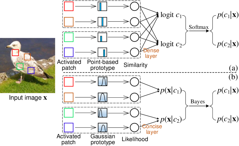
Figure 1: (a) Existing methods in ProtoPNet family are softmax-based discriminative classifiers that learn point-based prototypes. (b) Our new mixture of Gaussian-distributed prototypes is learned from a generative strategy, with classification achieved via the Bayes’ theorem using the class-conditional data density modelled by the prototype distributions.

Current prototypical part networks [5, 9, 36, 60] rely on a discriminative classifier optimised with point-based learning techniques that provide specific values for prototypes. Such a classifier produces logits (weighted sum of similarity scores) that are passed on to a softmax function to obtain the class probability given an input image, i.e., $p(c|\mathbf{x})$, as shown in Fig. 1(a). Though straightforward and easy to implement, the learned prototypes have limited representation power due to their sparsity, potential redundancy, and inability to represent prototype variability. Also, these point-based models are challenging for the detection of Out-of-Distribution (OoD) samples [2, 33], a capability being studied for prototypical-part interpretable methods [36].

In contrast to discriminative models, generative models are trained with distribution-based learning techniques to model the class-conditional data density $p(\mathbf{x}|c)$, where the classification decision is made according to Bayes’ theorem. Interestingly, the distributions learned from generative models can address the representational power issues of prototypical part networks, particularly with regards to the learning of prototypes. For instance, if instead of learning point-based prototypes, we learn distribution-based prototypes, then they will occupy denser regions in the latent prototype space, as in Fig. 1(b). Also, such distribution-based prototypes can be naturally used to detect OoD samples. Hence, it is interesting to study how to integrate the generative learning of distribution-based prototypes into the training of prototypical part networks.

In this paper, we present a novel generative paradigm to learn prototype distributions for interpretable image classification. Specifically, our method learns a Mixture of Gaussian-distributed Prototypes (MGProto) to represent each visual class in a generative way. For inference, the model assigns the class prediction to the category whose mixture of Gaussian-distributed prototypes can best describe the input image. MGProto enables the learning of more powerful prototype representations since each learned prototype will have a measure of variability, which naturally reduces sparsity given the spread of the distribution around each prototype. We also leverage a prototype diversity objective function in MGProto to reduce prototype redundancy. Furthermore, the prior probability learned for each prototype is utilised to prune prototypes in order to improve model compactness. Incidentally, since prototypes are represented by distributions, we propose a new strategy for detecting OoD samples, which as mentioned above, is becoming an important feature of ProtoPNet models [36]. To summarise, our major contributions are:

1. We provide the new generative learning of prototype distributions for interpretable image classification, with the MGProto framework, where the prototype distributions are represented by Gaussian mixture model (GMM) to acquire more powerful prototypical representations.

2. We promote model compactness by adaptively pruning prototypical Gaussian components with a low prior and reduce prototype redundancy by enlarging within-class prototype distances in the optimisation of GMMs.

3. Given that our prototypes are represented by distributions, we propose an effective prototype-based method to detect OoD samples, which is becoming an important feature of ProtoPNet models.

Our results on CUB-200-2011, Stanford Cars, Stanford Dogs, and Oxford-IIIT Pets show that MGProto outperforms current state-of-the-art (SOTA) methods in terms of image classification and OoD detection performances. Moreover, our MGProto exhibits promising results for different measures of interpretability.

2 Related Work

2.1 Interpretability with Prototypes

Post-hoc strategies have been widely used for model interpretation, e.g., saliency maps [49, 67, 47], explanation surrogates [32, 68, 48], and counterfactual examples [15, 50, 17]. On the other hand, prototype-based interpretable models provide another interesting way to access the model’s inner workings. ProtoPNet [5] is the original work that adopts a number of class-specific prototypes for interpretable image classification. Built upon ProtoPNet, TesNet [61] introduces the orthonormal transparent basis concepts, and Deformable ProtoPNet [9] proposes spatially-deformable prototypes to better adapt to the variations of objects. Meanwhile, some works focus on reducing the number of prototypes, so that a user needs to inspect only a handful of prototypes [44, 45]. Other efforts have been made to integrate the prototype learning with neural decision trees [35, 24], visual transformers [64, 24], K-nearest neighbour [53], and knowledge distillation [19]. Recently, ProtoPDebug [4] presents a concept-level debugger to correct the confounded prototypes. PIP-Net [36] pretrains prototypes in a self-supervised way and regularises the prototype-class connection sparsity for compact explanation. ST-ProtoPNet [60] leverages both support and trivial prototypes for ensembled classification interpretations. In [16], two objective evaluation metrics (i.e., consistency and stability) are proposed to assess the prototype-based interpretability.

Promisingly, prototype-based interpretable methods are being applied in critical tasks beyond the ones in computer vision [21, 52, 57, 46, 14, 18]. However, these existing models are trained with discriminative learning techniques that produce a point-based estimate of prototypes, resulting in prototypes with specific values that have limited representation power. The method ProtoVAE [13] proposes to learn image-level prototypes regularised by a variational auto-encoder (VAE) that is trained to reconstruct the input image, but the learned prototypes in ProtoVAE still depend on discriminative point-based learning techniques.

2.2 Gaussian Mixture Model

Gaussian Mixture Model (GMM) [41] is a probabilistic model for representing data distributions with a mixture of Gaussian components, which has been extensively explored in a variety of applications [62, 31, 66, 65, 7]. To estimate GMM’s parameters, the Expectation–Maximisation (EM) algorithm [34] is often harnessed by iterating between evaluating the responsibility using the current parameters (E-step) and maximising the data log-likelihood (M-step). Although offering closed-form solutions, the standard EM algorithm cannot ensure diverse Gaussian components, which is important for prototype-based interpretability since it requires non-redundant prototypes. In [31], the GMMSeg method exploits GMMs with a Sinkhorn EM algorithm for semantic segmentation, but it assumes uniform priors over Gaussian components, which conflicts with our prototype pruning strategy. A recent work [63] utilises GMMs to explain deep features and produces faithful post-hoc explanations, which is notably different from our gray-box model. In this paper, we show that the interpretable prototypes in ProtoPNet family can be formulated as GMMs to explicitly capture the underlying class-conditional data density. Also, to reduce prototype redundancy, we integrate a new term into the objective function to learn a mixture of diverse Gaussian-distributed prototypes.

3 ProtoPNet Preliminaries

Let $\mathbf{x}\in\mathcal{X}\subset\mathbb{R}^{H\times W\times R}$ denote an image with size $H\times W$ and $R$ colour channels, and $\mathbf{y}\in\mathcal{Y}\subset\{0,1\}^{C}$ is the one-hot image-level class label with $\mathbf{y}_{c}=1$ if the image label is $c$ and $\mathbf{y}_{c}=0$ otherwise. A typical ProtoPNet classifies an image $\mathbf{x}$ using the following three sequential steps:

1) The embedding step feeds $\mathbf{x}$ to a feature backbone $f_{\theta_{\textbf{bcb}}}:\mathcal{X}\to\mathcal{Z}$, parameterised by $\theta_{\textbf{bcb}}$, to extract deep features $\mathbf{z}\in\mathcal{Z}\subset\mathbb{R}^{\bar{H}\times\bar{W}\times\bar{D}}$, which is passed on to several add-on layers $f_{\theta_{\textbf{add}}}:\mathcal{Z}\to\mathcal{F}$, parameterised by $\theta_{\textbf{add}}$, to extract feature maps $\mathbf{F}\in\mathcal{F}\subset\mathbb{R}^{\bar{H}\times\bar{W}\times D}$, where $\bar{H}\leq H$, $\bar{W}\leq W$ and $D$ denotes the number of feature channels.

2) The prototype-activating step uses a set of learnable prototypes $\mathcal{P}=\{\mathbf{p}_{m}\}_{m=1}^{M\times C}$ to represent prototypical object parts (e.g., claws and beaks from class “bird”) in training images, where each of $C$ classes has $M$ prototypes and $\mathbf{p}_{m}\in\mathbb{R}^{1\times 1\times D}$. This step computes $M\times C$ similarity maps between the feature map $\mathbf{F}$ and prototypes $\mathcal{P}$: $\mathbf{S}_{m}^{(i,j)}={\mathsf{sim}}(\mathbf{F}^{(i,j)},\mathbf{p}_{m})$, where $i\in\{1,...,\bar{H}\}$, $j\in\{1,...,\bar{W}\}$, $\mathbf{F}^{(i,j)}\in\mathbb{R}^{1\times 1\times D}$, and $\mathsf{sim(\cdot,\cdot)}$ is a similarity metric, e.g., cosine similarity [9]. These similarity maps are then transformed into $M\times C$ similarity/activation scores from the max-pooling: $\mathbf{s}_{m}(\mathbf{x})=\Big{\{}\underset{i,j}{\max}\;\mathbf{S}_{m}^{(i,j)}\Big{\}}_{m=1}^{M\times C}$.

3) The aggregating step computes the logit of class $c$ by accumulating $\mathbf{s}_{m}(\mathbf{x})$ via a dense linear layer as in Fig. 1(a): logit${}_{c}=\sum_{m=1}^{M\times C}\boldsymbol{\pi}_{m}^{c}\mathbf{s}_{m}(\mathbf{x})$, where $\boldsymbol{\pi}^{c}\in\mathbb{R}^{MC\times 1}$ is the layer’s connection weight with class $c$. A softmax function is applied to the output logits of all classes to predict the posterior class probability $p(c|\mathbf{x};\theta,\mathcal{P},\boldsymbol{\pi})$, where $\theta=\left\{\theta_{\textbf{bcb}},\theta_{\textbf{add}}\right\},\mathcal{P},\boldsymbol{\pi}$ are parameters of ProtoPNet.

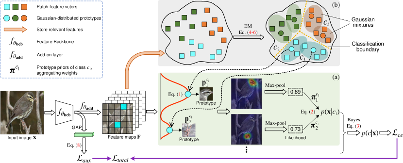
Figure 2: The overall framework of the MGProto method. For a given image $\mathbf{x}$, the model backbone (e.g., ResNet) extracts deep features $f_{\theta_{\textbf{bcb}}}(\mathbf{x})$ that are then fed to the add-on layer $f_{\theta_{\textbf{add}}}$ to obtain feature maps $\mathbf{F}$. (a) The case-based interpretation is achieved by comparing the feature representation $\mathbf{F}$ with the mixture of Gaussian-distributed prototypes (for simplicity, we illustrate only two prototypes for class $c_{1}$). Bayes’ theorem is then utilised to derive the posterior class probability $p(c|\mathbf{x})$ for making the classification predictions and computing the cross-entropy loss $\mathcal{L}_{ce}$. (b) For each class, the mixture of Gaussian-distributed prototypes is estimated by a modified EM algorithm to encourage prototype diversity. An auxiliary loss $\mathcal{L}_{aux}$ is applied on $f_{\theta_{\textbf{bcb}}}(\mathbf{x})$ to improve the backbone’s feature extraction ability.

4 Mixture of Gaussian-distributed Prototypes

Our proposed MGProto method, as illustrated in Fig. 2, represents ProtoPNet’s prototypes with Gaussian Mixture Models (GMMs). First, we formulate the similarity computation between the feature maps $\mathbf{F}$ and Gaussian prototype distributions $\{\mathbf{p}^{c}_{m},\mathbf{\Sigma}^{c}_{m}\}_{m,c=1}^{M,C}$, with:

where $i\in\{1,...,\bar{H}\}$, $j\in\{1,...,\bar{W}\}$, $\mathbf{p}_{m}\in\mathbb{R}^{D}$ and $\mathbf{\Sigma}_{m}\in\mathbb{R}^{D\times D}$ denote the prototype’s mean and covariance, respectively. The class-wise maximum similarity scores are obtained with $\mathbf{s}^{c}_{m}(\mathbf{x})=\Big{\{}\underset{i,j}{\max}\;\mathbf{S}_{m}^{(i,j),c}\Big{\}}_{m=1}^{M}$. In MGProto, we also have multiple prototypes (e.g., $M$ = 10) for each class $c$, whose similarity scores are accumulated by weighted sum in the aggregating layer. This naturally inspires us to derive the GMM formulation, which captures the class-conditional data density with:

$$\begin{split}p(\mathbf{x}|c)&=\sum_{m=1}^{M}\boldsymbol{\pi}_{m}^{c}\mathbf{s}_{m}^{c}(\mathbf{x})=\sum_{m=1}^{M}\boldsymbol{\pi}_{m}^{c}\underset{i,j}{\max}\;\mathbf{S}_{m}^{(i,j),c}\\ &=\sum_{m=1}^{M}\boldsymbol{\pi}_{m}^{c}\underset{i,j}{\max}\;\mathcal{N}(\mathbf{F}^{(i,j)};\mathbf{p}_{m}^{c},\mathbf{\Sigma}_{m}^{c}),\end{split}$$ (2)

where the aggregating weights $\boldsymbol{\pi}^{c}$ are mixture weights in GMM to quantify the prototype importance, we call them prototype priors. In Eq. (2), the nature of mixtures enables the prototype distributions of class $c$ to collaboratively represent the underlying data density of that class.

It is worth noting that our MGProto utilises a concise aggregating layer (see Fig. 1(b) and Fig. 2), i.e, $\boldsymbol{\pi}^{c}\in\mathbb{R}^{M\times 1}$, instead of $\boldsymbol{\pi}^{c}\in\mathbb{R}^{MC\times 1}$, as in the previous methods [5, 61, 9, 60] described in Sec. 3. Compared with the previous dense layer, such a concise layer not only introduces the prototype-class connection sparsity to reduce the explanation size [36], but also prevents the classification logit of a class from being disturbed by prototypes of other classes [16]. More importantly, our MGProto further offers an appealing property from the Gaussian mixture formulation: the prototype priors (aggregating weights) satisfy: $\sum_{m=1}^{M}\boldsymbol{\pi}_{m}^{c}=1$, for each class $c$. This allows us to prune low-prior prototypes to improve model compactness.

According to Bayes’ theorem, the posterior class probability $p(c|\mathbf{x})$ is computed as:

$$p(c|\mathbf{x})=\frac{p(\mathbf{x}|c)p(c)}{\sum_{c^{\prime}=1}^{C}p(\mathbf{x}|c^{\prime})p(c^{\prime})}=\frac{p(\mathbf{x}|c)}{\sum_{c^{\prime}=1}^{C}p(\mathbf{x}|c^{\prime})}$$ (3)

by assuming $p(c)=\frac{1}{C}$, as in many works in literature [38, 42, 39]. Relying on this assumption, the core of MGProto is to accurately estimate the class-conditional distributions $p(\mathbf{x}|c)$ defined in Eq. (2), which is trained with generative learning techniques.

The well-known EM algorithm [34] can be employed to jointly estimate the prototypes means $\mathbf{p}^{c}$, covariances $\mathbf{\Sigma}^{c}$, and priors $\boldsymbol{\pi}^{c}$ for each class $c$. Nevertheless, the standard EM algorithm does not guarantee diverse characteristics of the estimated prototypes, which is crucial for prototype-based interpretability [61, 9, 60]. Therefore, we introduce a modified EM strategy to encourage prototype diversity during their learning, as detailed in Sec. 4.1.

4.1 Diverse Prototype Distribution Learning

In this section, we explain the learning of the class-wise GMM parameters, denoted by $\phi^{c}=\left\{\mathbf{p}_{m}^{c},\mathbf{\Sigma}_{m}^{c},\boldsymbol{\pi}_{m}^{c}\right\}_{m=1}^{M}$, which will represent the diverse prototype distributions.

To help GMMs accurately represent the underlying prototype distributions, we harness a memory bank [6] to make full use of a large set of feature representations instead of considering only the few samples present in a mini-batch. The memory bank is represented by a class-wise queue $\mathcal{B}^{c}\in\mathbb{R}^{N\times D}$ that stores the relevant class-wise features from previous training samples processed during learning, where $N$ is the memory capacity for each class $c$, and a feature $\mathbf{f}$ is denoted by one of the $\bar{H}\times\bar{W}$ feature vectors of the feature representation $\mathbf{F}$. More specifically, the queue $\mathcal{B}^{c}$ is formed by taking a training image from class $c$, and storing its $M$ most relevant features consisting of the nearest features to the $M$ prototypes of class $c$ (see Fig. 2), rather than storing all $\bar{H}\times\bar{W}$ features. The memory is discarded after training, thus introducing no extra overhead for testing.

For each class $c$, we use the the memory queue $\mathcal{B}^{c}$ to learn the GMM parameters $\phi^{c}$, via the EM algorithm. The E-step computes the responsibility that each feature $\mathbf{f}_{n}^{c}\in\mathcal{B}^{c}$, where $n\in\{1,...,N\}$, is generated by $m$-th Gaussian-distributed prototype of class $c$:

$$\gamma_{n,m}^{c}=\frac{\boldsymbol{\pi}_{m}^{c}\mathcal{N}(\mathbf{f}_{n}^{c};\mathbf{p}_{m}^{c},\mathbf{\Sigma}_{m}^{c})}{\sum_{m=1}^{M}\boldsymbol{\pi}_{m}^{c}\mathcal{N}(\mathbf{f}_{n}^{c};\mathbf{p}_{m}^{c},\mathbf{\Sigma}_{m}^{c})}.$$ (4)

The standard EM algorithm’s M-step provides a closed-form solution [41] that does not enforce the learning of diverse prototypes, which can result in redundant prototypes, an issue observed in our experiments. Motivated by [28], in this paper we tackle this issue by explicitly incorporating a prototype diversity loss term into the M-step, as follows:

where the first term aims to maximise the log-likelihood over all samples in the memory $\mathcal{B}^{c}$ and the second term improves prototype diversity by encouraging large within-class prototype distances in an exponential form. Note that Eq. (5) has no closed-form solution, so we update $\{\mathbf{p}_{m}^{c},\mathbf{\Sigma}_{m}^{c}\}_{m=1}^{M}$ via gradient descent. The update of the prototype priors $\boldsymbol{\pi}_{m}^{c}$ can still rely on the closed-form solution:

$$\boldsymbol{\pi}_{m}^{c*}=\frac{1}{N}\sum_{i=1}^{N}\gamma_{n,m}^{c}.$$ (6)

The training of the GMM parameters $\phi^{c}$ involves iterative loops between the E-step and M-step. Since the memory progressively evolves during training, we obverse that only few iterations (e.g., 3 in this work) are needed to achieve good convergence for the EM algorithm.

4.2 Optimisation Objective

The overall training objective of our proposed MGProto method within a mini-batch $\mathcal{K}$ is defined as:

$$\mathcal{L}_{total}=\frac{1}{|\mathcal{K}|}\sum_{(\mathbf{x},\mathbf{y})\in\mathcal{K}}\mathcal{L}_{ce}(\mathbf{x},\mathbf{y})+\lambda\mathcal{L}_{aux}(\mathbf{x},\mathbf{y}),$$ (7)

where $\lambda>0$ is a hyper-parameter, and $\mathcal{L}_{ce}(\cdot)$ is the cross-entropy (CE) loss. Also in Eq. (7), the Proxy-Anchor [23] auxiliary loss $\mathcal{L}_{aux}(\cdot)$ enhances the features extracted by the model backbone, as suggested by [53]. Specifically, we use a Global Average Pooling (GAP) operator to condense the deep features $\mathbf{z}=f_{\theta_{\textbf{bcb}}}(\mathbf{x})$ into the embedding $\mathbf{e}=\mathsf{GAP}(\mathbf{z})\in\mathbb{R}^{\bar{D}}$, and the loss is computed with:

where $\mathcal{Q}=\{\mathbf{q}_{1},...,\mathbf{q}_{C}\}$ denotes the set of learnable proxies for all classes, and $\mathcal{Q}^{+}\subset\mathcal{Q}$ is the set of proxies for the classes present in the mini-batch $\mathcal{K}$. The set of embeddings $\mathbf{e}$ of the samples, computed with $\mathsf{GAP(\cdot)}$, from the mini-batch $\mathcal{K}$ is divided into $\mathcal{E}_{\mathbf{q}}^{+}$ and $\mathcal{E}_{\mathbf{q}}^{-}$ containing the batch embeddings with the same class or different class as the proxy $\mathbf{q}$, respectively. Also in Eq. (8), the function $\mathsf{sim}(\cdot,\cdot)$ computes the cosine similarity, $\delta$ and $\alpha$ are hyper-parameters ($\delta=0.1$ and $\alpha=32$, according to [23]).

4.3 Training Process and Prototype Projection

The training process of MGProto alternates between two steps: 1) optimising the model backbone and add-on layer’s parameters $\theta=\left\{\theta_{\textbf{bcb}},\theta_{\textbf{add}}\right\}$ using Eq. (7), with GMM’s parameters frozen; and 2) estimating the GMM’s parameters $\phi^{c}=\left\{\mathbf{p}_{m}^{c},\mathbf{\Sigma}_{m}^{c},\boldsymbol{\pi}_{m}^{c}\right\}_{m=1}^{M}$ for each class $c\in\{1,...,C\}$ via the modified EM using Eq. (4), Eq. (5) and Eq. (6), with the model backbone and add-on layers frozen. A detailed training algorithm for MGProto is provided in the supplementary material.

To ensure that the prototypes are represented by actual training image patches, as in [5, 61, 9, 53], we replace each of the $M$ means of the learned Gaussian-distributed prototypes by the most similar training image feature from class $c$, after the model’s training, with:

$$\ \mathbf{p}_{m}^{c}\leftarrow\arg\max_{\mathbf{F}\in\mathcal{F}^{c},i\in\{1,...,\bar{H}\},j\in\{1,...,\bar{W}\}}\mathbf{S}_{m}^{(i,j),c},$$ (9)

where $\mathcal{F}^{c}$ represents the set of all features extract from the training images belonging to class $c$, and $m\in\{1,...,M\}$. This makes the prototypes semantically-transparent to realise case-based interpretability, i.e., classifying samples based on their similarity to the training image prototypes.

4.4 MGProto for OoD Detection

MGProto explicitly models the class-conditional data distribution $p(\mathbf{x}|c)$, which naturally enables to detect OoD samples by computing the overall data likelihood:

$$p(\mathbf{x})=\sum_{c=1}^{C}p(\mathbf{x}|c)p(c)\propto\sum_{c=1}^{C}p(\mathbf{x}|c).$$ (10)

Based on Eq. (10) above, anomalous OoD samples have low likelihood $p(\mathbf{x})$, which in practice means that $\mathbf{x}$ will be far from prototypes of all classes and, consequently, will not fit well the prototype distributions of any classes.

5 Experiments

We evaluate our method on three standard benchmark datasets: CUB-200-2011 [55], Stanford Cars [26], and Stanford Dogs [20]. Additionally, to follow the same setting of OoD detection in PIP-Net [36], we also use Oxford-IIIT Pets [37] for fair comparison with [36]. Images are resized to 224 $\times$ 224 and we use online augmentations [35, 53] during training. Please refer to the supplementary material for more implementation details.

5.1 Experimental Settings

We evaluate our method on various CNN backbone architectures: VGG16 (V16), VGG19 (V19), ResNet34 (R34), ResNet50 (R50), ResNet152 (R152), DenseNet121 (D121), and DenseNet161 (D161), which are all pre-trained on ImageNet [8], except for ResNet50 on CUB that is pre-trained on iNaturalist [54]. We employ the same prototype dimension $D=64$ and prototype number $M=10$ for all backbones and datasets. Following [9, 36], we obtain more fine-grained feature maps with $\bar{H}=\bar{W}=14$ by dropping the final max-pooling layer in the backbones. Then two add-on $1\times 1$ convolutional layers (without activation function) are appended to reduce the number of feature channels to the prototype dimension $D$. The memory capacity $N$ is set to 800, 1000, 2000, 2000 for CUB, Cars, Dogs, and Pets, respectively. In Eq. (7), we have $\lambda$ = 0.5.

We assess different facets of interpretability by computing the following measures on CUB using full images: 1) Consistency score quantifies how consistently each prototype activates the same human-annotated object part [16]; 2) Purity of prototypes, similar to the consistency score, evaluates the extent that the top-10 image patches for a prototype can encode the same object-part [36]; 3) Stability score measures how robust the object part activation is when noise is added to an image input [16]; 4) Outside-Inside Relevance Ratio (OIRR) calculates the ratio of mean activation outside the object to those within the object, using ground-truth object segmentation masks [29]; and 5) Deletion AUC (DAUC) computes the degree in the probability drop of the predicted class as more and more activated pixels are erased [40]. The consistency, purity, and stability are part-level measures, OIRR is an object-level measure, and DAUC is a model-level measure based on causality.

5.2 Classification Accuracy

Tab. 1 shows the comparison results with the state-of-the-art method among variants of ProtoPNet using full images of CUB, where the Baseline denotes a non-interpretable black-box model. As we can see, with 10 prototypes per class, our method trained with the $\mathcal{L}_{total}$ in Eq. (7) consistently achieves the best accuracy for all CNN backbones. Note that by only using the cross-entropy loss $\mathcal{L}_{ce}$, our method can still outperform other models [5, 61, 9, 60, 16] that utilise not only cross-entropy loss but also extra regularisation losses (e.g., cluster and separation). We observe that the accuracy is further improved when the auxiliary loss is adopted (i.e., forming $\mathcal{L}_{total}$ in Eq. (7)), verifying its usefulness in helping the CNN backbone to acquire better feature extraction ability. Our method can also outperform the recent ProtoKNN [53], when trained using a smaller number of prototypes (2 prototypes per class, 400 in total).

Method	# Proto.	V16	V19	R34	R50	R152	D121	D161
Baseline	n.a.	70.9	71.3	76.0	78.7	79.2	78.2	80.0
ProtoKNN [53]	1×1p, 512	77.2	77.6	77.6	87.0	80.6	79.8	81.4
MGProto($\mathcal{L}_{total}$)	1×1p, 400	77.9	78.6	80.0	86.7	81.4	80.5	82.0
ProtoPNet [5]	1×1p, 10pc	70.3	72.6	72.4	81.1	74.3	74.0	75.4
TesNet [61]	1×1p, 10pc	75.8	77.5	76.2	86.5	79.0	80.2	79.6
Deformable [9]	2×2p, 10pc	75.7	76.0	76.8	86.4	79.6	79.0	81.2
ST-ProtoPNet [60]	1×1p, 10pc	76.2	77.6	77.4	86.6	78.7	78.6	80.6
Huang et al. [16]	1×1p, 10pc	76.4	77.7	77.8	86.4	79.9	80.4	81.4
MGProto($\mathcal{L}_{ce}$)	1×1p, 10pc	77.8	78.6	79.6	86.5	80.6	80.7	81.8
MGProto($\mathcal{L}_{total}$)	1×1p, 10pc	78.3	79.2	81.1	87.1	82.0	81.1	82.3

Table 1: Classification accuracy (%) on full images of CUB-200-2011 by different approaches, where 1×1p, 10pc denotes 1$\times$1 spatial shape of prototypes and 10 prototypes per class. Our results are averaged across five runs with random seeds.

Tab. 2 shows the classification results on Cars by different methods that use the same model backbone of ResNet50. Following previous studies [5, 45, 53], we also crop the images using the provided bounding boxes and evaluate our method on the cropped version of Cars. As evident, our MGProto exhibits the best classification accuracy, when using both full and cropped images. Results in Tab. 3 show the superiority of our MGProto on Stanford Dogs.

In Fig. 3, we visually illustrate all 10 prototypes for four (out of 200) classes from CUB, and the T-SNE representations of prototypes and training features from our MGProto. It can be observed that: 1) large-prior prototypes, which dominate the decision making, are always from high-density distribution regions (in T-SNE) and can localise well the object (bird) parts; 2) background prototypes tend to have a low prior and come from the low-density distribution regions; 3) some prototypes localise the object parts but have a low prior, suggesting that those object parts may not be important for identifying that class.

Fig. 4 shows the prototype variability by sampling a “pseudo” prototype from the prototype distribution and visualising with its nearest training image patch. It is seen that as the sampled pseudo prototypes move further away from the mean, they gradually exhibit a changing appearance.

Data	ProtoPNet [5]	ProtoTree [35]	ProtoPool [45]	PIP-Net [36]	ProtoKNN [53]	MGProto
BBox	88.4	89.2	88.9	90.2	90.9	91.5
Full	86.1	86.6	86.3	86.5	–	88.7

Table 2: Classification accuracy (%) on Stanford Cars based on ResNet50. “BBox” and “Full” denote that a method is trained and tested on bounding-box cropped and full images, respectively.

Method	# Proto.	V16	V19	R34	R50	R152	D121	D161
Baseline	n.a.	75.6	77.3	81.1	83.1	85.2	81.9	84.1
ProtoPNet [5]	1×1p, 10pc	70.7	73.6	73.4	76.4	76.2	72.0	77.3
TesNet [61]	1×1p, 10pc	74.3	77.1	80.1	82.4	83.8	80.3	83.8
Deformable [9]	3×3p, 10pc	75.8	77.9	80.6	82.2	86.5	80.7	83.7
ST-ProtoPNet [60]	1×1p, 10pc	74.2	77.2	80.8	84.0	85.3	79.4	84.4
MGProto	1×1p, 10pc	75.0	78.5	82.5	85.4	87.0	81.2	85.2

Table 3: Classification accuracy (%) on full images of Stanford Dogs by competing approaches using different CNN backbones.

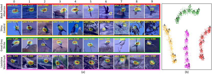
Figure 3: Visual prototypes (a) and T-SNE results (b) of our MGProto method from CUB-200-2011. These visual prototypes are marked with a yellow box in the activation maps, with the corresponding prototype prior provided. In T-SNE, we show the prototypes (stars), their ID (numbers), and training features (dots) stored in the memory queue. The figure randomly shows 4 out of 200 classes from a ResNet34-based model, where each colour indicates a different class and for each class we display all 10 prototypes.

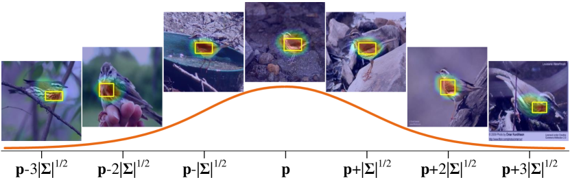
Figure 4: Visual variability of prototypes by sampling from the Gaussian prototype distribution. Note that the prototype mean $\mathbf{p}$ is the same as in Fig. 3 (ID: 4, class: Louisiana Waterthrush).

5.3 Prototype Pruning

Method	# Initial Proto.	ResNet34			ResNet152
		# Proto.	% Pruned	Accuracy	# Proto.	% Pruned	Accuracy
ProtoPShare [44]	2000	400	80.0	78.5 $\rightarrow$ 74.7	1000	50.0	75.5 $\rightarrow$ 73.6
ProtoPNet [5]	2000	1655	17.3	79.2 $\rightarrow$ 79.5	1734	13.3	78.3 $\rightarrow$ 78.6
MGProto†	2000	1997	0.15	81.1 $\rightarrow$ 81.1	1988	0.60	82.0 $\rightarrow$ 82.0
MGProto (ours)	2000	1600	20.0	81.1 $\rightarrow$ 81.2	1600	20.0	82.0 $\rightarrow$ 82.1
	2000	1200	40.0	81.1 $\rightarrow$ 80.9	1200	40.0	82.0 $\rightarrow$ 82.0
	2000	800	60.0	81.1 $\rightarrow$ 80.8	800	60.0	82.0 $\rightarrow$ 81.8
	2000	400	80.0	81.1 $\rightarrow$ 80.6	400	80.0	82.0 $\rightarrow$ 81.6
	2000	200	90.0	81.1 $\rightarrow$ 80.1	200	90.0	82.0 $\rightarrow$ 80.9

Table 4: Classification accuracy (%) of different pruned models on CUB-200-2011, where our MGProto is pruned by only keeping prototypes with a high prior for each class. MGProto^†: we use the previous pruning strategy [5] in our MGProto. % Pruned denotes the ratio between the pruned prototypes to the initial ones.

To improve model compactness, we prune prototypes based on their prior $\boldsymbol{\pi}^{c}$, i.e., keep only important prototypes with top-$k$ priors for each class ($k$ = 1, 2, 4, 6, 8). This can avoid choosing complicated class-wise pruning thresholds. We also attempt to apply the previous purity-based pruning strategy from [5] to our MGProto, but only a few prototypes are pruned, as shown in Tab. 4, indicating that the previous pruning strategy is improper to our method, mostly because our prototypes have large purity, as shown in Tab. 7. Fortunately, our prior-based strategy enables MGProto to greatly reduce the number of prototypes and maintain a high classification accuracy. Interestingly, pruning 20% of prototypes slightly leads to accuracy increases. When using a very large pruning rate (e.g., 90%), our method exhibits a tolerable performance drop (about 1% in both backbones). This is because the large-prior prototypes always lie in high-density regions of the data distribution (see Fig. 3(b)), capturing enough representative semantic information. From Fig. 3(a), the small-prior prototypes tend to be from the background image regions and less important object parts.

5.4 OoD Detection

Method	CUB-Cars	CUB-Pets	Cars-CUB	Cars-Pets	Pets-CUB	Pets-Cars
PIP-Net [36]	1.1	8.1	7.8	5.6	12.9	0.9
MGProto	0.04	8.1	3.5	3.0	8.8	0.02

Table 5: FPR95 (%) on OoD detection for each ID-OoD pair, by computing the false positive rate of OoD samples when the true positive rate of ID samples is at 95%. The models are trained using only ID samples.

As a generative model, MGProto can naturally detect OoD samples while perform interpretable classification for in-distribution (ID) samples. Following PIP-Net [36], we perform experiments on CUB, Cars, and Pets (e.g., choose one dataset as ID and the other two as OoD) and report the FPR95 metric. Notice that, for the OoD detection problem, our MGProto needs only one threshold for the data likelihood $p(\mathbf{x})$ in Eq. (10), which is different from PIP-Net demanding sophisticated per-class thresholds [36]. Tab. 5 displays the OoD detection experiments based on ResNet50 backbone, with results showing that our method outperforms PIP-Net by a large margin in most tasks. For example, when trained on Cars and classifying 95% of the testing Cars images as ID samples, MGProto detects 96.5% of CUB images as OoD, while PIP-Net only detects 92.2% under the same setting. Fig. 5 shows the likelihood histogram for the task of CUB as ID, Cars and Pets as OoD, revealing that our MGProto has high likelihood for ID samples and low likelihood for OoD samples. Fig. 5 also suggests that CUB images have larger semantic distance to Cars than Pets, which is aligned with our human intuition.

It is also worth mentioning that our MGProto achieves a higher classification accuracy (92.0%) than PIP-Net (88.5%) on Pets test set, when both methods utilise the same ResNet50 backbone and are trained on Pets.

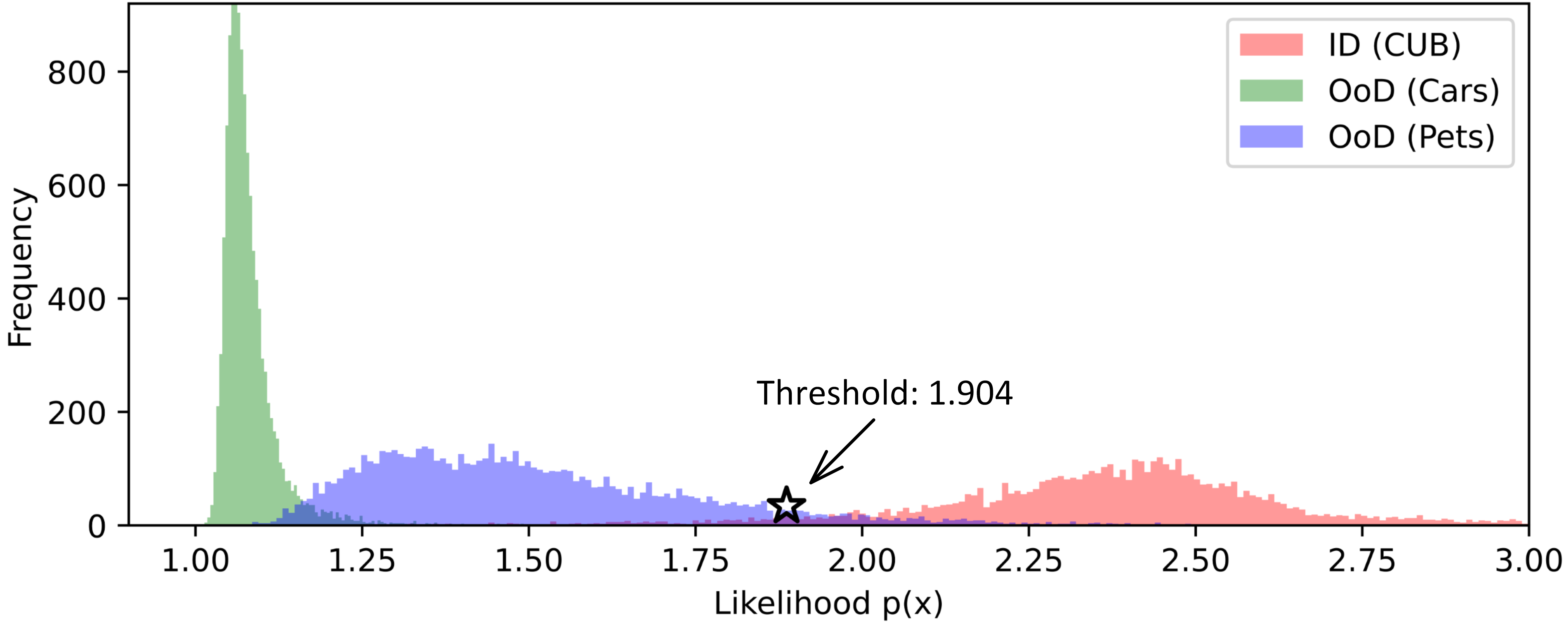
Figure 5: Histograms of the data likelihood $p(\mathbf{x})$ computed from Eq. (10) for ID test set and OoD train + test set. MGProto can abstain from making a decision for an OoD sample if the data likelihood $p(\mathbf{x})$ is smaller than a threshold marked by the star.

5.5 Interpretability Quantification

Tab. 6 shows the interpretability comparison of different methods. MGProto has the highest consistency score, indicating that the object parts activated by our prototypes are consistent across different images. This is likely because our method holistically learns prototypes from a large set of relevant feature representations, allowing them to consistently capture comprehensive semantics. MGProto also achieves competitive stability score. Interestingly, our method has high a stability score of 65.91% at the beginning of training, which gradually decreases and converges to 46.06%. We hypothesise that this is in part due to the ImageNet pre-trained CNN backbone being quite robust to the input noise. The lowest OIRR score demonstrates that our MGProto relies more on the object region and less on the background context to support classification decision. The DAUC result indicates that our model produces interpretations that best influence its classification predictions. We also compute the prototype purity in Tab. 7, showing that the prototypes by our method have a high degree of purity, i.e., each prototype focuses on semantically-consistent object parts among different images.

Metric	ProtoPNet  [5]	Deformable  [9]	TesNet  [61]	ST-ProtoPNet  [60]	Huang et al.  [16]	MGProto
Consistency ($\uparrow$)	45.29	57.87	60.75	74.08	80.45	92.90
Stability ($\uparrow$)	42.23	43.91	39.20	44.96	46.30	46.06
OIRR ($\downarrow$)	37.26	28.68	38.97	28.09	33.65	23.70
DAUC ($\downarrow$)	7.39	5.99	5.86	5.74	4.30	3.52

Table 6: Quantitative interpretability results (%) on full images of CUB test set, where all models are based on VGG19 backbone.

Method	Purity (train) $\uparrow$	Purity (test) $\uparrow$
ProtoPNet [5]	0.44 ± 0.21	0.46 ± 0.22
ProtoTree [35]	0.13 ± 0.14	0.14 ± 0.16
ProtoPShare [44]	0.43 ± 0.21	0.43 ± 0.22
ProtoPool [45]	0.35 ± 0.20	0.36 ± 0.21
PIP-Net [36]	0.63 ± 0.25	0.65 ± 0.25
MGProto	0.69 ± 0.21	0.68 ± 0.21

Table 7: Prototype purity (%) on train and test sets of CUB using full images, where all models are based on ResNet50 backbone.

5.6 Ablation Study

Prototype diversity loss in M-step. In Eq. (5), we add a diversity loss term to improve the distances of within-class prototype pairs. To validate its effectiveness, we give an ablation study on CUB and Cars, with results given in Tab. 8. Note both the classification accuracy and the mean $L_{2}$ distances between prototypes increase when including the diversity term in the M-step, suggesting that diversity is critical to enable classification accuracy improvements. We provide the visual comparison of prototypes by the closed-form EM and diverse EM in the supplementary material.

CUB (ResNet34)				Cars (Full images, ResNet50)
Closed-form EM		Diverse EM (ours)		Closed-form EM		Diverse EM (ours)
Accuracy	Distance	Accuracy	Distance	Accuracy	Distance	Accuracy	Distance
79.8	0.0475	81.1	0.1456	86.8	0.0814	88.7	0.1578

Table 8: Ablation analysis of the prototype diversity loss term defined in Eq. (5), where we show both the classification accuracy (%) and the average $L_{2}$ distance of within-class prototype pairs.

Memory capacity. External memory is used for GMMs to accurately learn the prototype distributions. Here, we study the effect of memory capacity $N$ on the classification accuracy. The result in Fig. 6(a) shows that the external memory contributes to higher accuracy, compared with learning from only mini-batch samples. However, a memory with too large capacity evolves too slowly and the presence of early-trained features can deteriorate performance, while a small-capacity memory cannot store enough features for a reliable GMM estimation. Hence, we choose the memory capacity $N$ = 800 for CUB (for other datasets we select $N$ based on the class sample ratio relative to CUB).

Sensitivity of $\lambda$. We also investigate the the sensitivity of our MGProto method to the hyperparameter $\lambda$ in Eq. (7), with results shown in Fig. 6(b). The classification accuracy is generally stable for $\lambda$ ranging from 0.1 to 2. If $\lambda$ is too small, the model backbone cannot extract effective features, whereas if $\lambda$ is too large, the cross-entropy loss will be overpowered, resulting in lower accuracy. We thus set $\lambda$ = 0.5 for all backbones and datasets.

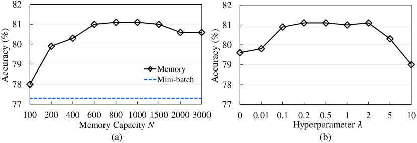
Figure 6: Effects of (a) memory capacity $N$ and (b) hyper-parameter $\lambda$ on the classification accuracy, using a ResNet34-based MGProto model on CUB-200-2011.

6 Conclusion

This work presented MGProto, a generative method for learning a mixture of Gaussian-distributed prototypes for interpretable image classification. Different from current point-based prototypes, our prototype distributions are represented by Gaussian mixture models to acquire more prototypical representation power. Relying on the prior-based pruning strategy, MGProto can substantially reduce the explanation size (consequently promote model compactness) while keeping a high classification accuracy. Additionally, MGProto can effectively detect OoD samples using the overall data likelihood. Since our prototypes are learned to model the underlying data distributions, it is possible to sample from the distributions and generate new examples for model explanation, e.g., counterfactual examples. We plan to explore this in our future work.

References

- Alvarez Melis and Jaakkola [2018] David Alvarez Melis and Tommi Jaakkola. Towards robust interpretability with self-explaining neural networks. Advances in Neural Information Processing Systems, 31, 2018.
- Bernardo et al. [2007] JM Bernardo, MJ Bayarri, JO Berger, AP Dawid, D Heckerman, AFM Smith, and M West. Generative or discriminative? getting the best of both worlds. Bayesian statistics, 8(3):3–24, 2007.
- Böhle et al. [2022] Moritz Böhle, Mario Fritz, and Bernt Schiele. B-cos networks: Alignment is all we need for interpretability. In Proceedings of the IEEE/CVF Conference on Computer Vision and Pattern Recognition, pages 10329–10338, 2022.
- Bontempelli et al. [2023] Andrea Bontempelli, Stefano Teso, Katya Tentori, Fausto Giunchiglia, and Andrea Passerini. Concept-level debugging of part-prototype networks. In International Conference on Learning Representations, 2023.
- Chen et al. [2019] Chaofan Chen, Oscar Li, Daniel Tao, Alina Barnett, Cynthia Rudin, and Jonathan K Su. This looks like that: deep learning for interpretable image recognition. Advances in Neural Information Processing Systems, 32, 2019.
- Chen et al. [2020] Ting Chen, Simon Kornblith, Mohammad Norouzi, and Geoffrey Hinton. A simple framework for contrastive learning of visual representations. In International Conference on Machine Learning, pages 1597–1607. PMLR, 2020.
- Cheng et al. [2020] Zhengxue Cheng, Heming Sun, Masaru Takeuchi, and Jiro Katto. Learned image compression with discretized gaussian mixture likelihoods and attention modules. In Proceedings of the IEEE/CVF conference on computer vision and pattern recognition, pages 7939–7948, 2020.
- Deng et al. [2009] Jia Deng, Wei Dong, Richard Socher, Li-Jia Li, Kai Li, and Li Fei-Fei. Imagenet: A large-scale hierarchical image database. In 2009 IEEE Conference on Computer Vision and Pattern Recognition, pages 248–255. Ieee, 2009.
- Donnelly et al. [2022] Jon Donnelly, Alina Jade Barnett, and Chaofan Chen. Deformable protopnet: An interpretable image classifier using deformable prototypes. In Proceedings of the IEEE/CVF Conference on Computer Vision and Pattern Recognition, pages 10265–10275, 2022.
- Fang et al. [2017a] Leyuan Fang, David Cunefare, Chong Wang, Robyn H Guymer, Shutao Li, and Sina Farsiu. Automatic segmentation of nine retinal layer boundaries in oct images of non-exudative amd patients using deep learning and graph search. Biomedical optics express, 8(5):2732–2744, 2017a.
- Fang et al. [2017b] Leyuan Fang, Chong Wang, Shutao Li, Jun Yan, Xiangdong Chen, and Hossein Rabbani. Automatic classification of retinal three-dimensional optical coherence tomography images using principal component analysis network with composite kernels. Journal of Biomedical Optics, 22(11):116011–116011, 2017b.
- Fang et al. [2019] Leyuan Fang, Chong Wang, Shutao Li, Hossein Rabbani, Xiangdong Chen, and Zhimin Liu. Attention to lesion: Lesion-aware convolutional neural network for retinal optical coherence tomography image classification. IEEE transactions on medical imaging, 38(8):1959–1970, 2019.
- Gautam et al. [2022] Srishti Gautam, Ahcene Boubekki, Stine Hansen, Suaiba Salahuddin, Robert Jenssen, Marina Höhne, and Michael Kampffmeyer. Protovae: A trustworthy self-explainable prototypical variational model. Advances in Neural Information Processing Systems, 35:17940–17952, 2022.
- Gerstenberger et al. [2023] Michael Gerstenberger, Steffen Maaß, Peter Eisert, and Sebastian Bosse. A differentiable gaussian prototype layer for explainable fruit segmentation. In IEEE International Conference on Image Processing (ICIP), pages 2665–2669. IEEE, 2023.
- Goyal et al. [2019] Yash Goyal, Ziyan Wu, Jan Ernst, Dhruv Batra, Devi Parikh, and Stefan Lee. Counterfactual visual explanations. In International Conference on Machine Learning, pages 2376–2384. PMLR, 2019.
- Huang et al. [2023] Qihan Huang, Mengqi Xue, Wenqi Huang, Haofei Zhang, Jie Song, Yongcheng Jing, and Mingli Song. Evaluation and improvement of interpretability for self-explainable part-prototype networks. In Proceedings of the IEEE/CVF International Conference on Computer Vision, pages 2011–2020, 2023.
- Kenny and Keane [2021] Eoin M Kenny and Mark T Keane. On generating plausible counterfactual and semi-factual explanations for deep learning. In Proceedings of the AAAI Conference on Artificial Intelligence, pages 11575–11585, 2021.
- Kenny et al. [2023] Eoin M Kenny, Mycal Tucker, and Julie Shah. Towards interpretable deep reinforcement learning with human-friendly prototypes. In International Conference on Learning Representations, 2023.
- Keswani et al. [2022] Monish Keswani, Sriranjani Ramakrishnan, Nishant Reddy, and Vineeth N Balasubramanian. Proto2proto: Can you recognize the car, the way i do? In Proceedings of the IEEE/CVF Conference on Computer Vision and Pattern Recognition, pages 10233–10243, 2022.
- Khosla et al. [2011] Aditya Khosla, Nityananda Jayadevaprakash, Bangpeng Yao, and Fei-Fei Li. Novel dataset for fine-grained image categorization: Stanford dogs. In Proc. CVPR Workshop on Fine-grained Visual Categorization (FGVC), 2011.
- Kim et al. [2021] Eunji Kim, Siwon Kim, Minji Seo, and Sungroh Yoon. Xprotonet: diagnosis in chest radiography with global and local explanations. In Proceedings of the IEEE/CVF Conference on Computer Vision and Pattern Recognition, pages 15719–15728, 2021.
- Kim and Canny [2017] Jinkyu Kim and John Canny. Interpretable learning for self-driving cars by visualizing causal attention. In Proceedings of the IEEE International Conference on Computer Vision, pages 2942–2950, 2017.
- Kim et al. [2020] Sungyeon Kim, Dongwon Kim, Minsu Cho, and Suha Kwak. Proxy anchor loss for deep metric learning. In Proceedings of the IEEE/CVF conference on computer vision and pattern recognition, pages 3238–3247, 2020.
- Kim et al. [2022] Sangwon Kim, Jaeyeal Nam, and Byoung Chul Ko. Vit-net: Interpretable vision transformers with neural tree decoder. In International Conference on Machine Learning, pages 11162–11172. PMLR, 2022.
- Koh and Liang [2017] Pang Wei Koh and Percy Liang. Understanding black-box predictions via influence functions. In International Conference on Machine Learning, pages 1885–1894. PMLR, 2017.
- Krause et al. [2013] Jonathan Krause, Michael Stark, Jia Deng, and Li Fei-Fei. 3d object representations for fine-grained categorization. In Proceedings of the IEEE International Conference on Computer Vision Workshops, pages 554–561, 2013.
- Krizhevsky et al. [2017] Alex Krizhevsky, Ilya Sutskever, and Geoffrey E Hinton. Imagenet classification with deep convolutional neural networks. Communications of the ACM, 60(6):84–90, 2017.
- Kwok and Adams [2012] James Kwok and Ryan P Adams. Priors for diversity in generative latent variable models. Advances in Neural Information Processing Systems, 25, 2012.
- Lapuschkin et al. [2016] Sebastian Lapuschkin, Alexander Binder, Grégoire Montavon, Klaus-Robert Muller, and Wojciech Samek. Analyzing classifiers: Fisher vectors and deep neural networks. In Proceedings of the IEEE Conference on Computer Vision and Pattern Recognition, pages 2912–2920, 2016.
- LeCun et al. [2015] Yann LeCun, Yoshua Bengio, and Geoffrey Hinton. Deep learning. Nature, 521(7553):436–444, 2015.
- Liang et al. [2022] Chen Liang, Wenguan Wang, Jiaxu Miao, and Yi Yang. Gmmseg: Gaussian mixture based generative semantic segmentation models. Advances in Neural Information Processing Systems, 35:31360–31375, 2022.
- Lundberg and Lee [2017] Scott M Lundberg and Su-In Lee. A unified approach to interpreting model predictions. Advances in Neural Information Processing Systems, 30, 2017.
- Mackowiak et al. [2021] Radek Mackowiak, Lynton Ardizzone, Ullrich Kothe, and Carsten Rother. Generative classifiers as a basis for trustworthy image classification. In Proceedings of the IEEE/CVF Conference on Computer Vision and Pattern Recognition, pages 2971–2981, 2021.
- Moon [1996] Todd K Moon. The expectation-maximization algorithm. IEEE Signal processing magazine, 13(6):47–60, 1996.
- Nauta et al. [2021] Meike Nauta, Ron van Bree, and Christin Seifert. Neural prototype trees for interpretable fine-grained image recognition. In Proceedings of the IEEE/CVF Conference on Computer Vision and Pattern Recognition, pages 14933–14943, 2021.
- Nauta et al. [2023] Meike Nauta, Jörg Schlötterer, Maurice van Keulen, and Christin Seifert. Pip-net: Patch-based intuitive prototypes for interpretable image classification. In Proceedings of the IEEE/CVF Conference on Computer Vision and Pattern Recognition, pages 2744–2753, 2023.
- Parkhi et al. [2012] Omkar M Parkhi, Andrea Vedaldi, Andrew Zisserman, and CV Jawahar. Cats and dogs. In 2012 IEEE conference on computer vision and pattern recognition, pages 3498–3505. IEEE, 2012.
- Pearl [1988] Judea Pearl. Probabilistic reasoning in intelligent systems: networks of plausible inference. Morgan kaufmann, 1988.
- Peng et al. [2004] Fuchun Peng, Dale Schuurmans, and Shaojun Wang. Augmenting naive bayes classifiers with statistical language models. Information Retrieval, 7:317–345, 2004.
- Petsiuk et al. [2018] Vitali Petsiuk, Abir Das, and Kate Saenko. Rise: Randomized input sampling for explanation of black-box models. arXiv preprint arXiv:1806.07421, 2018.
- Reynolds et al. [2009] Douglas A Reynolds et al. Gaussian mixture models. Encyclopedia of biometrics, 741(659-663), 2009.
- Rish et al. [2001] Irina Rish et al. An empirical study of the naive bayes classifier. In IJCAI 2001 workshop on empirical methods in artificial intelligence, pages 41–46, 2001.
- Rudin [2019] Cynthia Rudin. Stop explaining black box machine learning models for high stakes decisions and use interpretable models instead. Nature Machine Intelligence, 1(5):206–215, 2019.
- Rymarczyk et al. [2021] Dawid Rymarczyk, Łukasz Struski, Jacek Tabor, and Bartosz Zieliński. Protopshare: Prototypical parts sharing for similarity discovery in interpretable image classification. In Proceedings of the 27th ACM SIGKDD Conference on Knowledge Discovery & Data Mining, pages 1420–1430, 2021.
- Rymarczyk et al. [2022] Dawid Rymarczyk, Łukasz Struski, Michał Górszczak, Koryna Lewandowska, Jacek Tabor, and Bartosz Zieliński. Interpretable image classification with differentiable prototypes assignment. In European Conference on Computer Vision, pages 351–368. Springer, 2022.
- Sacha et al. [2023] Mikołaj Sacha, Dawid Rymarczyk, Łukasz Struski, Jacek Tabor, and Bartosz Zieliński. Protoseg: Interpretable semantic segmentation with prototypical parts. In Proceedings of the IEEE/CVF Winter Conference on Applications of Computer Vision, pages 1481–1492, 2023.
- Selvaraju et al. [2017] Ramprasaath R Selvaraju, Michael Cogswell, Abhishek Das, Ramakrishna Vedantam, Devi Parikh, and Dhruv Batra. Grad-cam: Visual explanations from deep networks via gradient-based localization. In Proceedings of the IEEE International Conference on Computer Vision, pages 618–626, 2017.
- Shitole et al. [2021] Vivswan Shitole, Fuxin Li, Minsuk Kahng, Prasad Tadepalli, and Alan Fern. One explanation is not enough: structured attention graphs for image classification. Advances in Neural Information Processing Systems, 34:11352–11363, 2021.
- Simonyan et al. [2013] Karen Simonyan, Andrea Vedaldi, and Andrew Zisserman. Deep inside convolutional networks: Visualising image classification models and saliency maps. arXiv preprint arXiv:1312.6034, 2013.
- Teney et al. [2020] Damien Teney, Ehsan Abbasnedjad, and Anton van den Hengel. Learning what makes a difference from counterfactual examples and gradient supervision. In European Conference on Computer Vision, pages 580–599. Springer, 2020.
- Tjoa and Guan [2020] Erico Tjoa and Cuntai Guan. A survey on explainable artificial intelligence (xai): Toward medical xai. IEEE Transactions on Neural Networks and Learning Systems, 32(11):4793–4813, 2020.
- Trinh et al. [2021] Loc Trinh, Michael Tsang, Sirisha Rambhatla, and Yan Liu. Interpretable and trustworthy deepfake detection via dynamic prototypes. In Proceedings of the IEEE/CVF Winter Conference on Applications of Computer Vision, pages 1973–1983, 2021.
- Ukai et al. [2023] Yuki Ukai, Tsubasa Hirakawa, Takayoshi Yamashita, and Hironobu Fujiyoshi. This looks like it rather than that: Protoknn for similarity-based classifiers. In International Conference on Learning Representations, 2023.
- Van Horn et al. [2018] Grant Van Horn, Oisin Mac Aodha, Yang Song, Yin Cui, Chen Sun, Alex Shepard, Hartwig Adam, Pietro Perona, and Serge Belongie. The inaturalist species classification and detection dataset. In Proceedings of the IEEE Conference on Computer Vision and Pattern Recognition, pages 8769–8778, 2018.
- Wah et al. [2011] Catherine Wah, Steve Branson, Peter Welinder, Pietro Perona, and Serge Belongie. The caltech-ucsd birds-200-2011 dataset. 2011.
- Wang et al. [2020] Chong Wang, Yuxuan Jin, Xiangdong Chen, and Zhimin Liu. Automatic classification of volumetric optical coherence tomography images via recurrent neural network. Sensing and Imaging, 21:1–15, 2020.
- Wang et al. [2022a] Chong Wang, Yuanhong Chen, Yuyuan Liu, Yu Tian, Fengbei Liu, Davis J McCarthy, Michael Elliott, Helen Frazer, and Gustavo Carneiro. Knowledge distillation to ensemble global and interpretable prototype-based mammogram classification models. In International Conference on Medical Image Computing and Computer-Assisted Intervention, pages 14–24. Springer, 2022a.
- Wang et al. [2022b] Chong Wang, Zhiming Cui, Junwei Yang, Miaofei Han, Gustavo Carneiro, and Dinggang Shen. Bowelnet: Joint semantic-geometric ensemble learning for bowel segmentation from both partially and fully labeled ct images. IEEE Transactions on Medical Imaging, 42(4):1225–1236, 2022b.
- Wang et al. [2023a] Chong Wang, Yuanhong Chen, Fengbei Liu, Michael Elliott, Chun Fung Kwok, Carlos Peña-Solorzano, Helen Frazer, Davis James McCarthy, and Gustavo Carneiro. An interpretable and accurate deep-learning diagnosis framework modelled with fully and semi-supervised reciprocal learning. IEEE Transactions on Medical Imaging, 2023a.
- Wang et al. [2023b] Chong Wang, Yuyuan Liu, Yuanhong Chen, Fengbei Liu, Yu Tian, Davis McCarthy, Helen Frazer, and Gustavo Carneiro. Learning support and trivial prototypes for interpretable image classification. In Proceedings of the IEEE/CVF International Conference on Computer Vision, pages 2062–2072, 2023b.
- Wang et al. [2021] Jiaqi Wang, Huafeng Liu, Xinyue Wang, and Liping Jing. Interpretable image recognition by constructing transparent embedding space. In Proceedings of the IEEE/CVF International Conference on Computer Vision, pages 895–904, 2021.
- Wu et al. [2023] Linshan Wu, Zhun Zhong, Leyuan Fang, Xingxin He, Qiang Liu, Jiayi Ma, and Hao Chen. Sparsely annotated semantic segmentation with adaptive gaussian mixtures. In Proceedings of the IEEE/CVF Conference on Computer Vision and Pattern Recognition, pages 15454–15464, 2023.
- Xie et al. [2023] Zhouyang Xie, Tianxiang He, Shengzhao Tian, Yan Fu, Junlin Zhou, and Duanbing Chen. Joint gaussian mixture model for versatile deep visual model explanation. Knowledge-Based Systems, 280:110989, 2023.
- Xue et al. [2022] Mengqi Xue, Qihan Huang, Haofei Zhang, Lechao Cheng, Jie Song, Minghui Wu, and Mingli Song. Protopformer: Concentrating on prototypical parts in vision transformers for interpretable image recognition. arXiv preprint arXiv:2208.10431, 2022.
- Yang et al. [2019] Linxiao Yang, Ngai-Man Cheung, Jiaying Li, and Jun Fang. Deep clustering by gaussian mixture variational autoencoders with graph embedding. In Proceedings of the IEEE/CVF international conference on computer vision, pages 6440–6449, 2019.
- Yuan et al. [2020] Wentao Yuan, Benjamin Eckart, Kihwan Kim, Varun Jampani, Dieter Fox, and Jan Kautz. Deepgmr: Learning latent gaussian mixture models for registration. In Computer Vision–ECCV 2020: 16th European Conference, Glasgow, UK, August 23–28, 2020, Proceedings, Part V 16, pages 733–750. Springer, 2020.
- Zeiler and Fergus [2014] Matthew D Zeiler and Rob Fergus. Visualizing and understanding convolutional networks. In European Conference on Computer Vision, pages 818–833. Springer, 2014.
- Zhang et al. [2018] Quanshi Zhang, Ruiming Cao, Feng Shi, Ying Nian Wu, and Song-Chun Zhu. Interpreting cnn knowledge via an explanatory graph. In Proceedings of the AAAI Conference on Artificial Intelligence, 2018.