Tree-based Forecasting of Day-ahead Solar Power Generation from Granular Meteorological Features

Abstract. Accurate forecasts for day-ahead photovoltaic (PV) power generation are crucial to support a high PV penetration rate in the local electricity grid and to assure stability in the grid. We use state-of-the-art tree-based machine learning methods to produce such forecasts and, unlike previous studies, we hereby account for (i) the effects various meteorological as well as astronomical features have on PV power production, and this (ii) at coarse as well as granular spatial locations. To this end, we use data from Belgium and forecast day-ahead PV power production at an hourly resolution. The insights from our study can assist utilities, decision-makers, and other stakeholders in optimizing grid operations, economic dispatch, and in facilitating the integration of distributed PV power into the electricity grid.

Keywords. Electricity Markets, Forecasting, Machine Learning, Regression trees, Renewable Energy, Solar Energy

1 Introduction

The integration of energy production from Renewable Energy Sources (RES) in the grid is a crucial pathway to the global reduction of greenhouse gas emissions and fossil fuel production (Ouikhalfan et al.,, 2022). In this paper, we focus on solar energy, which is the second fastest-growing RES; indeed the total installed photovoltaic (PV) power capacity in the world has increased from 42 GW in 2010 to 1 TW in 2022 (Our World in Data,, 2023). However, despite the worldwide deployment of PV power and its contributions to a more sustainable future, the intermittent and volatile nature of solar energy poses considerably challenges to the operations of power grids. Accurate PV power forecasts then become crucial for energy suppliers to stabilize the grid, and to optimize solar unit commitments and economic dispatch (Zsiborács et al.,, 2021). We consider tree-based machine learning methods to deliver such forecasts at the hourly resolution of the next business day, thereby accounting for meteorological and astronomical effects along a fine-grained grid of spatial locations.

Electricity markets display several specific yet challenging attributes compared to other commodities. First, electricity is economically non-storable as supply and demand need to be in constant balance. Additionally, demand and supply are intricately tied to external weather variables and calendar factors, introducing complex dynamics rarely seen in other markets (Weron,, 2014). With the rise of RES including PV energy, the complexity of the electric power systems is aggravating, as they become more dependent on the variability of external weather conditions. As a consequence, electrical grids become more unstable, and the imbalance and instability between consumption and production increase (Jacobson et al.,, 2019). Imbalances between power generation and demand can lead to increased costs for suppliers, including activating backup power plants or purchasing electricity at higher prices during periods of supply shortage (Yu and Hong,, 2016). Conversely, when supply exceeds demand, suppliers can face disposal costs, including curtailing or selling excess electricity at lower prices, as well as the opportunity cost of unused generation capacity (Inman et al.,, 2013). Accurate PV power forecasts are therefore crucial for energy suppliers to balance their power portfolio and stabilize the grid. Besides, they also hold considerably value for developing clean energy power generation technology (Liu et al.,, 2020).

PV power forecast methods can be classified into two main categories: (i) physical methods and (ii) data-driven methods (as well as combinations thereof), see Antonanzas et al., (2016); Krishnan et al., (2023). Physical methods are built on analytical equations that characterize the PV power systems and typically use theoretical simulation models to calculate the output power of a PV system based on its main design parameters, irradiance forecasts and numerical weather predictions (NWP) (Duffie et al.,, 2020; Masters,, 2013). Data-driven methods include both statistical, such as standard or penalized regression models (Abuella and Chowdhury, 2015b, ; Tang et al.,, 2018) as well as machine learning (ML) methods that can capture complex non-linear relationships. ML methods for PV power generation forecasting range from state-of-the-art artificial neural networks (ANN, see e.g., Abuella and Chowdhury, 2015a, ; Leva et al.,, 2017; Kaushaley et al.,, 2023), over support vector machines (SVM, see e.g., Sharma et al.,, 2011; Zeng and Qiao,, 2013) to tree-based methods (see e.g., Voyant et al.,, 2017). For a recent comprehensive overview, we refer the reader to Krishnan et al., (2023). These approaches typically use historical PV data and external variables such as weather conditions to forecast future PV power output.

Data-driven methods have recently become more popular due to the availability of large data at solar stations. Recent work by Visser et al., (2019); Alkabbani et al., (2021), and the review by Sudharshan et al., (2022) show that data-driven ML methods typically deliver the most accurate PV power forecasts at short-term forecast horizons (up until 48 hours ahead). Among the ML methods, the review study in Voyant et al., (2017) as well as extensive empirical work by Zamo et al., (2014); Visser et al., (2019) point towards the superior performance of tree-based models, such as regression trees, random forest or boosting methods. These models also tend to be less complex and prone to overfitting compared to ANNs and SVMs (Voyant et al.,, 2017).

In this paper, we therefore focus on tree-based ML methods in the important area of day-ahead PV power forecasting (Wan et al.,, 2015). Hourly day-ahead forecasts are mostly used for daily generation plans, economic dispatching plans, and trading on the day-ahead electricity market (Han et al.,, 2019). Our work contributes to this literature strand by offering a comprehensive forecasting framework that assists utilities such as energy suppliers and decision-makers in improving their grid operations, clean power energy technology, and lowering barriers for the integration of distributed PV in the local electricity grid. Our framework is centered around three main pillars: (i) we investigate the performance of various tree-based ML methods, ranging from regression trees, over random forest, to gradient boosting. We deliberately opt for tree-based methods (over neural networks or deep learning methods) not only due to their superior performance in the recent PV power forecasting literature but also thanks due their robust and sophisticated implementations that are nowadays routinely available across standard software packages (see the recent discussion by Januschowski et al.,, 2022), which greatly facilitates their adoption in industry. (ii) We use a distinct set of meteorological and astronomical features combined with careful feature engineering to forecast PW power. We contribute to the literature by providing an extensive discussion, based on a careful examination of the literature on solar engineering, photovoltaic systems and meteorology, of features that are deemed to be important in the forecasting model. Finally, (iii) we allow the effects of the various features to vary along a granular spatial grid of locations.

We carefully assess forecast performance, from a statistical point of view by computing the Model Confidence Set (Hansen et al.,, 2011) to separate the best performing models from their competitors, as well as from a graphical point of view, by offering practitioners advice on a diverse set of visualizations one can use to assess different aspects of forecast performance. Furthermore, to quantify the importance of meteorological and astronomical features at selected locations, we suggest to track feature importance based on SHAP (SHapley Additive exPlanation) values, as proposed by Lundberg and Lee, (2017).

We apply our forecasting framework to Belgian hourly PV data over the period January 1st, 2019 to June 30th, 2023. To our knowledge, no previous research has examined aggregated PV power output forecasts constructed at a regional (i.e. country) level and from a diverse set of meteorological features available at a fine-grained spatial grid. Besides, Belgium has not yet been the primary focus in earlier studies on PV power forecasting, yet its unique energy landscape makes it an especially pertinent subject for study. The country’s ongoing energy transition, characterized by a move away from nuclear power and an increased emphasis on renewable sources, presents a compelling case for the necessity of accurate PV power forecasts. The Belgian climate, with its significant variability, underscores the importance of robust forecasting frameworks capable of handling such fluctuations. Furthermore, Belgium’s availability of detailed hourly PV data makes it an ideal candidate for applying and evaluating the proposed forecasting framework; the results obtained can offer valuable insights for other regions facing similar integration challenges.

The remainder of this paper is organized as follows. Section 2 introduces the data and describes the feature engineering steps. Section 3 discusses the ML methods that we use to forecast PV power. Section 4 introduces our forecast framework, including the different model configurations, as well as the overall training, validation, and test set-up. Section 5 presents the results, which comprise forecast performance of all models, and a feature importance study. Section 6 concludes.

2 Data and Feature Engineering

We aim to obtain accurate day-ahead PV power forecasts. To this end, consider the following model

$$Y=f(X)+\varepsilon,$$ (1)

where $Y$ is our target variable namely PV power, $X=(X_{1},X_{2},\dots,X_{p})$ is a vector of $p$ features, $f$ denotes the forecast function that connects the features to the target, and $\varepsilon$ is the error term.

Section 2.1 provides details on the PV power target, Section 2.2 on the meteorological and astronomical features. Table 1 presents an overview of all variables used throughout the paper, together with their abbreviations and corresponding data providers. Our time frame spans from January 1st, 2019 to June 30th, 2023, resulting in a total of $T=39,407$ hourly observations. Note that all time units are measured in local time, thereby accounting for the seasonal shifts between summer and winter time in accordance with the Daylight Saving Time policy in Belgium.

Table 1: Data description and data sources.

Abbreviation	Variable Description	Data Source
ASG	Aggregated Actual Solar Generation Belgium (MW)	Elia Group Belgium, nd
IC	Installed Capacity in Belgium (MW)	Elia Group Belgium, nd
SNR	Individual cell Surface Net Solar Radiation (J m-2)	Copernicus Climate Change Service, Climate Data Store, (2023)
SSD	Individual cell Surface Solar Radiation Downwards (J m-2)	Copernicus Climate Change Service, Climate Data Store, (2023)
T2m	Individual cell Temperature at 2m (Kelvin)	Copernicus Climate Change Service, Climate Data Store, (2023)
RH	Individual cell Relative Humidity (%)	Copernicus Climate Change Service, Climate Data Store, (2023)
WCI	Individual cell Wind Chill Index (∘C)	Copernicus Climate Change Service, Climate Data Store, (2023)
TCC	Individual cell Total Cloud Cover (0 - 1)	Copernicus Climate Change Service, Climate Data Store, (2023)
Zenith	Zenith (Degree Angle)	(N/A)
Azimuth	Azimuth (Degree Angle)	(N/A)

Note: The variables zenith and azimuth have no data source since they are constructed manually.

2.1 PV Power Output

We collect aggregated Actual Solar Generation (ASG) in Belgium from Elia Group Belgium, nd , which is the Transmission System Operator (TSO) of Belgium. Figure 1 presents hourly ASG, measured in Megawatts (MW) units, over the whole sample as well as over selected sub-samples to highlight typical seasonal patterns.

From Figure 1(a), one can see that there is an overall upward trend in Belgian ASG, due to the increase in PV power installed capacity over the last years (Wolniak and Skotnicka-Zasadzien,, 2022). Figure 1(b) highlights that ASG is typically lower in winter months than in summer months. Weekly and daily patterns can be observed from respectively Figure 1(c) and 1(d). Note, however, that these are also influenced by the time of the year.

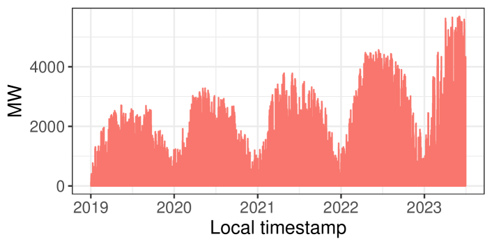
(a) ASG plot for the whole data set.

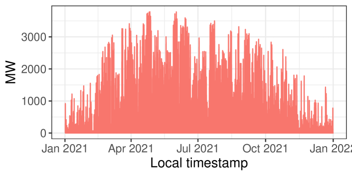
(b) ASG plot for 2021.

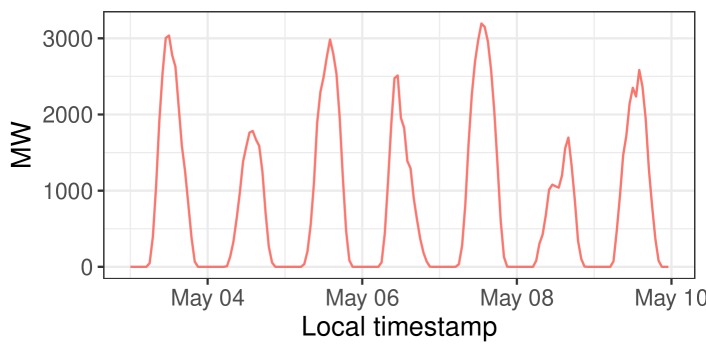
(c) ASG plot for May 3-9, 2021.

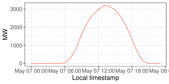
(d) ASG plot for May 7, 2021.

Figure 1: Actual Solar Generation (ASG) plots for different time periods.

We additionally collect Installed Capacity (IC) of PV power in Belgium in MW units from Elia Group Belgium, nd . Due to the granularity of the early data, we perform an interpolation, resulting in a smoothed capacity expansion curve illustrated in Figure 3 (with the original data represented by the green curve and the interpolated data by the blue curve). This approach ensures a more realistic depiction of capacity growth over time. The IC in Belgium increased considerably from 3,369 MW at the start of our sample to 7,593 MW at the end. For this reason, instead of forecasting raw ASG, we forecast a normalized version of ASG, in line with Bellinguer et al., (2020) who study wind energy output. By normalizing solar generation, the temporal evolution of the IC in Belgium is appropriately accounted for.

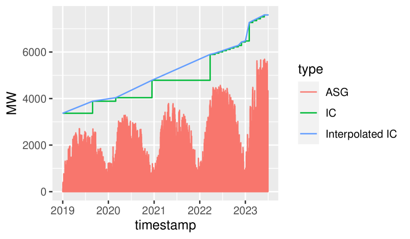
Figure 2: Construction of the Load Factor.

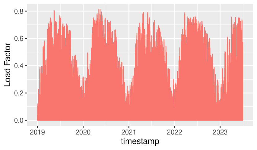
Figure 3: Load Factor (LF) time series.

The normalized ASG, also called Load Factor (LF), is then given by

$$Y^{*}_{t}=\frac{Y_{t}}{IC_{t}}\;,$$ (2)

where $Y_{t}$ is the ASG at time $t$, $IC_{t}$ the interpolated IC at time $t$. Figure 3 shows all time series used to construct the load factor, which, in turn, is visualized in Figure 3. The resulting load factor time series is scaled between zero and one and no longer displays the increasing trend of the raw ASG.

2.2 Features

2.2.1 Meteorological Features

We use six meteorological features that are known to be important for forecasting PV power (Son and Jung,, 2020; Abuella and Chowdhury, 2015b, ; Tang et al.,, 2018), namely Surface Net Solar Radiation (SNR), Surface Solar Radiation Downwards (SSD), Temperature at 2m (T2m), Relative Humidity (RH), Total Cloud Cover (TCC), and Wind Chill Index (WCI). These features cover Belgium’s spatial grid, including 62 locations as displayed in Figure 4. Figure 5 presents the six meteorological time series, averaged over the 62 locations. Below we explain the specific relationship between each of these six meteorological features and PV power, thereby supporting their inclusion in the forecasting model. A detailed description of how these variables are measured can be found in Hersbach et al., (2023); Copernicus Climate Change Service, Climate Data Store, (2023).

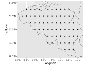
Figure 4: Grid points of the meteorological variables.

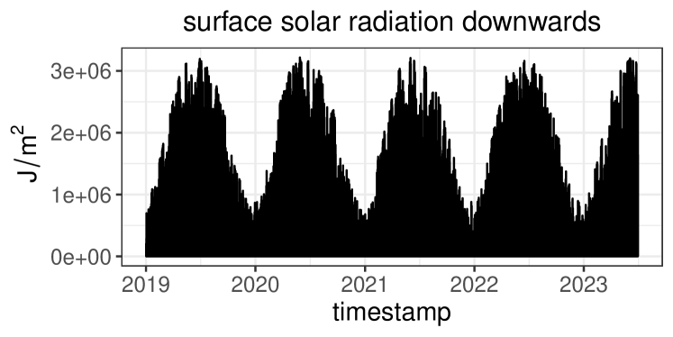
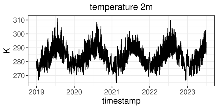
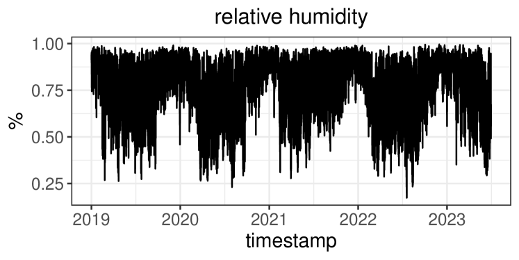
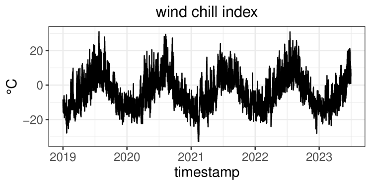
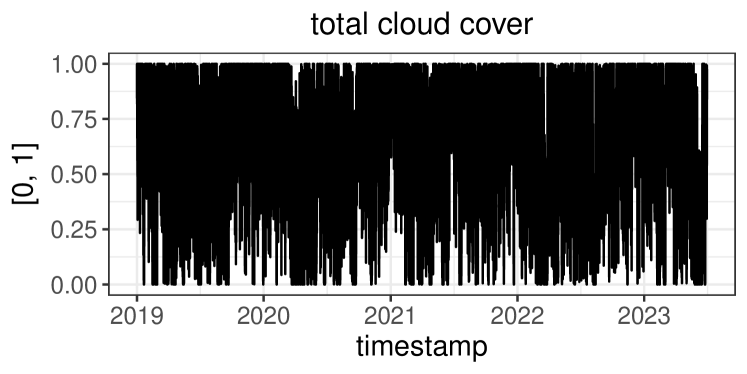
Figure 5: Meteorological features averaged over the 62 locations depicted in Figure 4.

Surface Solar Radiation.

Surface Net Solar Radiation (SNR) represents the amount of solar radiation reaching the surface of the Earth minus the amount reflected by the Earth’s surface, which is governed by the Albedo effect (Vokrouhlickỳ and Sehnal,, 1993). Indeed, radiation from the sun is partly reflected back to space by clouds and particles in the atmosphere, and some of the radiation is absorbed. Then, the difference between downward and reflected solar radiation is SNR. Surface Solar Radiation Downwards (SSD), on the contrary, gives the amount of solar radiation reaching the surface of the Earth and does not take into account the reflection of the sun by the Earth’s surface. The units of SNR and SSD are Joules per square meter (J m^-2). We consider these features since solar radiation has been shown to be the primary determinant of PV power generation (Son and Jung,, 2020; Abuella and Chowdhury, 2015a, ). Moreover, solar panels generate energy through the conversion of solar radiation, with direct solar radiation being regarded as one of the most promising sources of energy for this process (Baños et al.,, 2011).

Temperature.

The variable T2m denotes the air temperature 2 meters above the Earth’s surface, measured in Kelvin, which is a critical parameter for PV panel efficiency. Amajama and Mopta, (2016) show that air temperature operates within a range that can optimize the output of a PV panel. While solar radiation increases air temperature by transferring heat energy, it is also essential to note the inverse relationship between PV efficiency and excessive heat. Elevated temperatures may reduce the operational efficiency of PV systems due to overheating of the panels (Meral and Dinçer,, 2011).

Total Cloud Cover and Relative Humidity.

The variable TCC quantifies cloud coverage as the fraction of the sky obscured by clouds within a grid box, while RH is defined as the ratio of actual vapor pressure to the saturation vapor pressure, expressed as a percentage. TCC is anticipated to adversely affect PV power generation since cloudier conditions lead to a reduction in solar irradiation compared to clear skies, thereby diminishing PV output (Amajama and Oku,, 2016). Similarly for relative humidity, it is expected to indirectly impact PV output through its relation with solar radiation. Specifically, high RH can reduce the amount of sunlight that the panels can absorb, as photons are partially obstructed by denser water vapor in the atmosphere (Amajama and Oku,, 2016). Additionally, high humidity can lead to the formation of a thin layer of moisture on PV panels, further impairing their operational efficiency (Panjwani et al.,, 2017).

Wind Chill Index.

The last meteorological variable considered is WCI, which is a measure of the cooling effect of wind on the human body’s perception of temperature. It is the perceived decrease in air temperature felt by the body on exposed skin due to the flow of air (Lankford and Fox,, 2021). While this measure is based on temperature and wind speed concerning human comfort, it has applicability in assessing environmental conditions for PV systems. Wind speed, a component of WCI, can influence PV power output positively. Higher wind speeds may lead to a reduction in PV cell temperature, acting as a cooling mechanism and potentially enhancing efficiency (Schwingshackl et al.,, 2013). Hence, by including WCI as an additional feature, the effects of wind speed on PV power can be taken into account (Xydis,, 2013).

2.2.2 Astronomical Features

Finally, we use two astronomical features namely Zenith and Azimuth which are solar position variables utilized to track the position of the sun in the sky. Zenith represents the angle between the sun and the vertical direction of the observer, or alternatively, the angle between the sun and the point directly overhead. This angle is measured in degrees, where 0^∘ corresponds to the point directly overhead and 90^∘ represents the horizon. The Azimuth angle, on the other hand, is the angle between the due south and the projection of the sun’s position onto the horizon of the individual. It is measured in degrees from 0^∘ to 360^∘ in a clockwise direction from the due south (Reda and Andreas,, 2004).

The inclusion of Zenith and Azimuth as features in the PV output forecast model is important because they have an effect on the amount of radiation that reaches the surface of the earth. These variables explain the amount of radiation received at different times of the day and at different latitudes and thus directly impact the amount of solar energy produced at a given location Abdurrahman et al., (2019). Furthermore, these variables serve as a proxy for the temporal components or calendar effects that are related to ASG, as discussed in Section 2.1.

We compute the two astronomical variables in R (R Core Team,, 2023) using the solarPos package (Van doninck,, 2016) which implements the solar position algorithm as described in Reda and Andreas, (2004). The package calculates the position of the sun based on the latitude, longitude, and time of the observation in Julian time units. For our study, we apply this for the single location with coordinates $4.64$ ^∘E, $50.65$ ^∘N, as determined by averaging the longitude and latitude values from all locations depicted in Figure 4.

3 Tree-based Machine Learning Methods

This section reviews the Machine Learning (ML) methods that we use to forecast PV power to make the paper comprehensive. Section 3.1 outlines regression trees, Section 3.2 random forest and Section 3.3 (extreme) gradient boosting. For a more extensive introduction to each of these methods, we refer the interested reader to Hastie et al., (2009) (Chapters 9, 10 and 15).

3.1 Regression Trees

Regression trees (RT) partition the features space into smaller and smaller regions, and use local averages in each region to forecast the response. Assume the space is split into $M$ regions $R_{1},R_{2},\dots,R_{M}$, the forecast function is then given by ${f}(X)=\sum_{m=1}^{M}c_{m}I\{X\in R_{m}\}\,,$ where the regression model predicts $Y$ with a constant $c_{m}$ in region $R_{m}$. The estimate of $c_{m}$ is simply given by the average of the response values (in the training set) in region $R_{m}$, if one adopts the sum of squares as loss function. The regression tree can then be used to forecast the response for new observations by traversing down the tree from the root to a leaf node, based on the values of the features, and taking the average of the response value in the corresponding leaf node as forecast.

To train the RT, we use the greedy top-down recursive partitioning method explained in Breiman, (1984) and implemented in the R package rpart (Therneau and Atkinson,, 2022). Regression trees have three important tuning parameters. The first two, namely the maximum tree depth (MaxDepth) and minimum number of observations per terminal (leave) node ($\text{min}_{n}$), are used as stopping criteria when building the tree. The third one is the cost complexity parameter $\alpha$, which is used to prune the tree to reduce overfitting. In Section 4.2, we provide more details on how these parameters are tuned.

3.2 Random Forest

Random Forest (RF) is proposed by Breiman, (2001) as an ensemble method of multiple regression trees. Each tree is built by considering a random subset of features at each split of the tree, thereby providing diversity in the forecasts of the tree. By randomly selecting features as candidates for splitting, RFs can improve the variance reduction of bagging by reducing the correlation between the trees (thereby not increasing the variance too much). After growing a specified number of trees, the final forecast is simply the average of the forecasts across the large collection of de-correlated trees.

We use the ranger package (Wright and Ziegler,, 2017) in R to train the RF. The tuning parameters are the number of trees, the number of features to randomly select from per split (mtry) and the minimum number of observations per terminal node ($\text{min}_{n}$). We fix the number of trees at 600 and tune the other two parameters as will be detailed in Section 4.2.

3.3 Extreme Gradient Boosting

Finally, we consider Extreme Gradient Boosting (XGBoost), as proposed by Chen and Guestrin, (2016). XGBoost builds on the gradient boosting approach of Friedman, (2001) where the forecast function is constructed through a sequential ensemble of small regression trees, called weak learners, which together learn to build a strong learner. Each new learner is added based on the residual error obtained from the previous iteration of the weak learner. Gradient boosting then results in a one final tree, constructed as a weighted sum of trees, to be used for forecasting. XGBoost further optimizes the implementation of gradient boosting in terms of flexibility and computing time.

We use the XGBoost algorithm available in the xgboost package Chen et al., (2023) in R. For fair comparison to RF, we set the number of trees to 600. The hyperparameters requiring tuning are mtry, $\text{min}_{n}$, and MaxDepth (as discussed in Sections 3.1 and 3.2), the learning rate ($\eta$) which scales the contribution of each tree in the ensemble, the loss reduction ($\gamma$) which controls the model complexity of the trees, and finally SubSample which regulates the fraction of training data used for each boosting iteration to reduce overfitting.

4 Forecasting Framework

We present a comprehensive outline of our forecast framework. First, Section 4.1 offers an overview of the various model configurations we consider. Second, Section 4.2 outlines the design of the forecast study that is used for each model configuration. This includes the splitting of the sample into training, validation, and test sets, the process of hyperparameter tuning on the validation set, and the evaluation of forecast performance on the test set.

4.1 Model Configurations

We consider 24 model configurations, where a model configuration refers to a combination of (i) ML method used to estimate the forecast function $f$ in equation (1) (four considered methods), (ii) features used to predict the PV power output (two considered feature sets), and (iii) spatial grid of locations over which the meteorological features are computed (three considered grids). For the remainder of this paper, we refer to a model configuration as a specific combination in these three dimensions.

ML Method.

We investigate the performance of three different tree-based ML methods, namely regression trees (RT), random forest (RF) and extreme gradient boosting (XGBoost), see Section 3, and compare them to the linear regression (LR) model which serves as a simple baseline. All ML methods require tuning of their respective hyperparameters, which we discuss in Section 4.2.

Feature Set.

We consider two feature sets:

1. Surface Net Solar Radiation (SNR), Zenith, and Azimuth;

2. Surface Net Solar Radiation (SNR), Surface Solar Radiation Downwards (SSD), Temperature at 2m (T2m), Relative Humidity (RH), Wind Chill Index (WCI), Total Cloud Cover (TTC), Zenith, and Azimuth.

Feature set (a) is the simplest specification and only includes three features that directly relate to solar energy via radiation. This specification is based on domain-expertise and supported by the main findings, summarized in Section 2.2, that solar radiation and solar position have the largest impact on the PV output. By adding Azimuth and Zenith angles, we include a proxy for the time patterns visible in ASG and LF. In feature set (b), all meteorological variables introduced in Section 2.2 are additionally included. We are interested in investigating how these additional features drive forecasting power.

Spatial Grid of Locations.

We vary the number of spatial grid cells for all meteorological features to investigate the forecasting power of coarser as well as more granular grids. We consider three spatial grids. In the first coarse case, for each meteorological variable, we take the simple average over all 62 locations shown in Figure 4. For the other two more granular cases, we select specific grid points by $K$-means clustering, thereby varying the number of clusters $K$. The centroids $c$ from each of the resulting clusters $C$ indicate the most representative locations. We then select the grid points that are closest to these centroids as key locations. The optimization problem is given by

$$\underset{\;\;\;C}{\text{arg min}}\sum_{i=1}^{K}\sum_{x\in C_{i}}d_{h}(x,c_{i})^{2}\;,$$ (3)

where $x$ are the coordinates of the 62 grid cells, $c_{i}$ is the centroid of the points in cluster $C_{i}$, and $d_{h}(.,.)$ is the Haversine distance (Hegde et al.,, 2016). The Haversine distance $d_{h}(.,.)$ between two coordinates $i$ and $j$ is calculated as

$$d_{h}(i,j) =R\times 2\times\text{{atan2}}\left(\sqrt{a},\sqrt{1-a}\right),$$

$$\text{{where}}\;\,a =\sin^{2}\left(\frac{\Delta\theta}{2}\right)+\cos(\theta_{i})\times\cos(\theta_{j})\times\sin^{2}\left(\frac{\Delta\lambda}{2}\right),$$

with $\theta_{i}=\text{{lat}}_{i}\times\frac{\pi}{180}$, $\theta_{j}=\text{{lat}}_{j}\times\frac{\pi}{180}$, $\Delta\theta=(\text{{lat}}_{j}-\text{{lat}}_{i})\times\frac{\pi}{180}$, $\Delta\lambda=(\text{{lon}}_{j}-\text{{lon}}_{i})\times\frac{\pi}{180}$, where $\text{{lat}}_{i}$ ($\text{{lon}}_{i}$) are the latitude (longitude) of coordinate $i$, similarly for coordinate $j$, and $R$ is the radius of the earth (Hegde et al.,, 2016).

For the granular spatial grids, the number of clusters is set to $K=5$ and $K=12$; the resulting clusters with the corresponding key locations obtained are visualized in Figures 7 and 7 respectively. We choose these values of $K$ as both cover the whole territory of Belgium, while still considerably reducing the dimensionality of the problem. The $K=5$ locations case gives a rough representation and thereby represents a simpler setting where the main geographical regions in Belgium are covered (as will be discussed in Section 5.2), while the $K=12$ locations case aims to investigate whether the increased complexity in terms of spatial grid points pays off in terms of improved forecast accuracy.

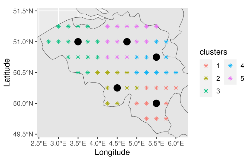
Figure 6: Grid points for $K=5$ clusters.

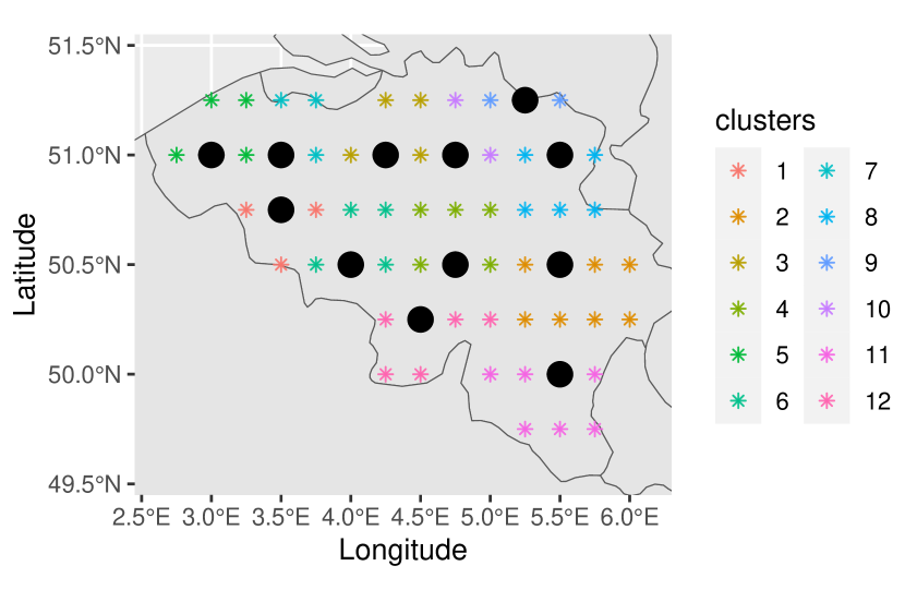
Figure 7: Grid points for $K=12$ clusters.

4.2 Design of the Forecast Study

To conduct our forecast exercise and compare forecast accuracy across the 24 model configurations, we split the data into a training, validation, and test set. The training set is used for training the ML models, the validation set for hyperparameter tuning and the test set for out-of-sample forecast performance evaluation.

The (initial) training set ranges from January 5, 2019, to January 4, 2021 (731 days); the validation set covers the period from January 5, 2021, to December 30, 2021 (360 days); and the test set encompasses the time period from January 1, 2022, to June 30, 2023 (545 days).

To optimize the tuning, training, and forecasting process, all night hours (when PV generation is typically zero) have been excluded from the dataset. Specifically, only the hours from 5 AM to 9 PM (hour 5 to 21) are retained. For the test set, which requires a complete 24-hour structure for evaluation, the omitted night hours are filled with zeros. This approach reflects the negligible solar power generation during these hours. Additionally, any negative forecasts generated by the models are adjusted to zero, as PV power output cannot be negative.

Finally, note that to validate and test the model, we intentionally included approximately one year and one and a half years of data, respectively, ensuring that the performance assessment and model selection include both winter and summer months. This approach allows us to account for the seasonal effects of ASG on forecast performance. We conduct our forecast exercise in R. The data set used in this paper as well as all replication files for the forecast study can be found on the GitHub page https://github.com/nberl/tree-based-dah-solar-forecast of the first author.

Validation Set: Hyperparameter Tuning.

To tune the hyperparameters of the ML methods on the validation set, we use a rolling window approach. We train the ML model on the most recent 731 days, and refresh the validation set every 30 days. The validation set thus consists of 12 consecutive slices, each spanning 30 days as visualized in Figure 9. For each slice, the blue segment represents the training data whereas the red segment represents the validation data. When training a particular ML model, we do this using a grid of hyperparameters for the respective ML method– RT, RF or XGBoost, see Section 3.1. The hyperparameters of each ML method are summarized in Table 2. We start by selecting 25 candidate sets of hyperparameters by a space-filling Latin Hypercube Design (LHD). As such we effectively explore the search space with a smaller number of evaluations compared to an exhaustive regular grid search (Santner et al.,, 2003). Specifically, a LHD partitions each hyperparameter grid into equally spaced intervals and then randomly selects a single value from each interval. The selected values form a LHD which ensures that the sampled points are evenly distributed across the hyperparameter space. The key idea is thus to obtain a representative sample of the hyperparameter space while reducing redundancy. We use the LHD implementation in the dials package (Santner et al.,, 2003) in R. For each of the 25 candidates, we compute the root mean squared error (RMSE) across all time points of the validation sets, and finally select the best combination of hyperparameters which results in the lowest RMSE metric.

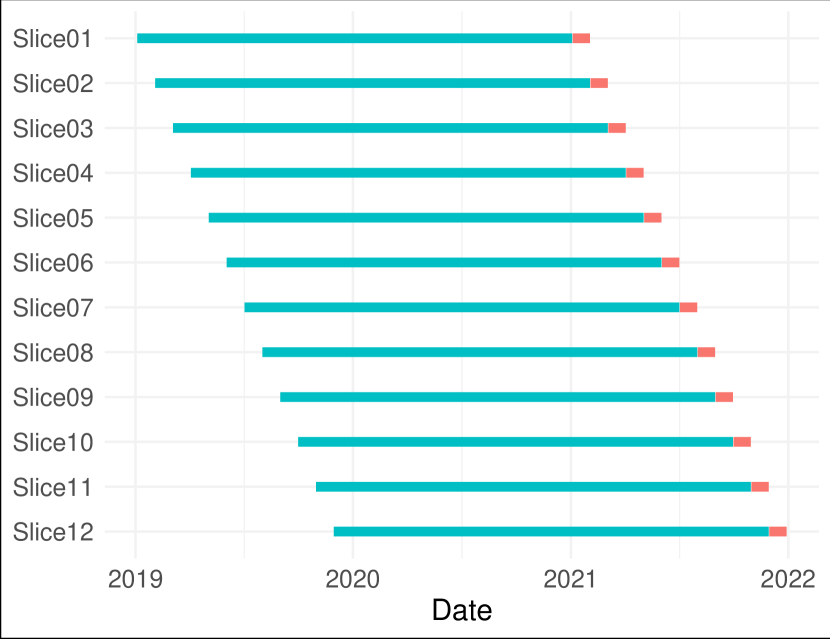
Figure 8: Rolling window procedure on the validation set.

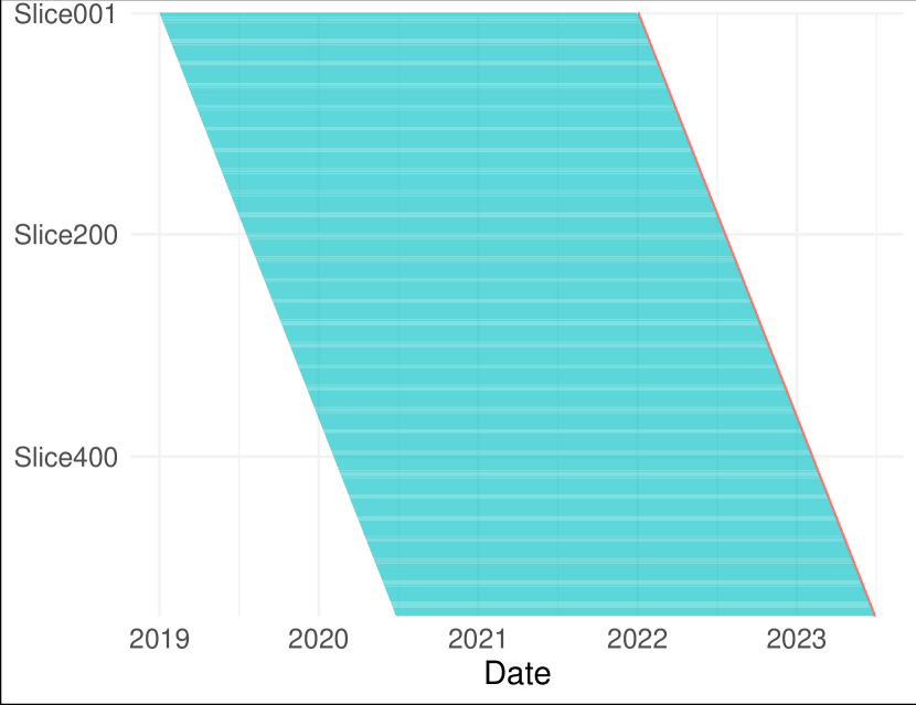
Figure 9: Rolling window procedure on the test set.

Table 2: Overview of hyperparameters per machine learning method.

Abbreviation	Definition	ML Method(s)
$\alpha$	Cost complexity for tree pruning	RT
MaxDepth	Maximum tree depth	RT, XGBoost
$\text{min}_{n}$	Minimum observations per node for further split	RT, RF, XGBoost
mtry	Number of randomly selected variables per split	RF, XGBoost
$\eta$	Learning rate or step size per ensemble iteration	XGBoost
$\gamma$	Penalty coefficient on number of leaf nodes	XGBoost
SubSample	Fraction of training data used each iteration	XGBoost
B	Number of base trees (fixed at 600)	RF, XGBoost

Test Set: Forecast Evaluation.

To compare the out-of-sample performance of the 24 model configurations on the test set, we use another rolling window set-up. We train each ML model with selected hyperparameters on the most recent three years, and compute day-ahead 24-hour PV power forecasts. The first training set then ranges from January 1, 2019 (the start of our dataset) to December 30, 2021. Afterwards in each iteration we move the training set one day forward until we reach the end of the sample. The first day in the test set is January 1, 2022. The test set consists of 545 consecutive slices, each spanning 24 hours of the day as visualized in Figure 9. For each slice, the blue segment represents the training data whereas the red segment represents the test data.

To evaluate the forecast performance of each model configuration, we compute three different forecast metrics across all time points of the test set. By comparing forecast performance across different metrics, we paint a broader picture when comparing the performance of the different model configurations. Specifically, we use the root mean square error (RMSE), mean absolute error (MAE), and a symmetric mean absolute percentage error (SMAPE) respectively defined as

$$\text{RMSE}=\sqrt{\sum_{t=1}^{N}\frac{(\hat{Y}_{t}-Y_{t})^{2}}{N}}\;,\ \text{MAE}=\frac{\sum_{t=1}^{N}|\hat{Y}_{t}-Y_{t}|}{N}\;,\,\ \text{and}\ \ \text{SMAPE}=2\frac{\sum_{t=1}^{N}|\hat{Y}_{t}-Y_{t}|}{\sum_{t=1}^{N}(\hat{Y}_{t}+Y_{t})}\;,$$

where $N$ denotes the number of time points in the test set, $\hat{Y}_{t}$ is the forecast of ASG at time $t$, and $Y_{t}$ is the ASG value at time $t$. The three performance metrics have been used extensively in PV power forecasting (Zhang et al.,, 2015; Krishnan et al.,, 2023). Note that each model forecasts the normalized ASG, as motivated in Section 2.1, but the actual forecast quantity of interest is ASG. We therefore first transform the forecasts back to the raw ASG-level using equation (2) before computing the forecast metrics.

5 Results

We presents the results in two parts. Section 5.1 presents the out-of-sample forecast results of all 24 model configurations. Section 5.2 zooms into the best performing model configurations and further compares them through a feature importance study based on SHAP values (Lundberg and Lee,, 2017).

5.1 Forecast Performance

We start by discussing overall forecast performance. Table 3 reports the out-of-sample RMSE, MAE, and SMAPE for the 24 tuned model configurations. A first glance at Table 3 reveals that, regardless of the chosen spatial grid and feature set, the ensemble methods RF and XGBoost obtain better forecast accuracy than the other methods, and this across all forecast metrics. Hence, non-parametric ML methods, where one does not have to worry about the functional form of the forecast function, and where feature selection and interaction are built-in, provide important forecast accuracy gains over simple, parametric LR models. This finding is consistent with recent advances in the day-ahead forecasting literature.

Table 3: Out-of-sample forecast performance for all 24 model configurations, defined through the combination of a particular ML method (rows), feature set (columns) and spatial grid (blocks across rows).

	Feature Set (a)				Feature Set (b)
Spatial Grid	Method	RMSE	MAE	SMAPE	RMSE	MAE	SMAPE
Average	LR	290	139	0.179	286	140	0.180
	RT	291	136	0.176	278	132	0.171
	RF	284	131	0.170*	266	131	0.169
	XGBoost	285	132	0.171	255	122	0.157
5 clusters	LR	285	137	0.177	277	139	0.178
	RT	290	137	0.178	284	135	0.175
	RF	275	128	0.166	252	119	0.154
	XGBoost	275	129	0.167	241*	117	0.151
12 clusters	LR	276	135	0.174	269	134	0.172
	RT	293	139	0.180	284	135	0.175
	RF	270	126	0.163	249	118	0.152**
	XGBoost	270	127	0.165	239**	115**	0.148

Note: The configurations included in the $99\%$ and $90\%$ MCS, computed per forecast metric separately, are identified by one and two asterisks respectively.

When comparing performance across the feature sets (a) and (b) and across the spatial grids, the differences in forecast performance are dependent on the ML method and the considered forecast metric. For the simple LR models, those models with feature set (b) perform slightly better based on the RMSE, but worse based on the MAE and SMAPE. Incorporating more locations in the linear regression model improves, overall, forecast performance. For the RT models, in contrast, increasing the number of spatial locations for meteorological variables generally leads to less accurate forecasts. For the best performing ML methods, RF and XGBoost, they clearly show improved forecast performance on all forecast metrics by adding complexity in terms of features as well as spatial locations. When comparing the RF models to the XGBoost models, the former yields slightly more accurate forecasts for more simple models with feature type set (a), while XGBoost performs better for more complex scenarios, i.e. feature type set (b) and 5 or 12 clusters for the spatial locations. Irrespective of the choice of forecast metric, the configuration XGBoost-(b)-12 yields the most accurate average forecasts on the considered test set, followed by the models XGBoost-(b)-5 and RF-(b)-12.

We now globally assess the significance of the differences in forecast performance among the 24 model configurations by computing the Model Confidence Set (Hansen et al.,, 2011). The MCS separates the set of best model configurations from their competitors for a given level of confidence. We calculate the MCS for each forecast metric separately. For our analysis, each forecast metric is computed on an observation-by-observation basis. Consequently, we use the squared error instead of the RMSE and the absolute error for the MAE. In the case of SMAPE, where the denominator can be zero, we set the error to zero when the value is undefined. To calculate the results for the 99% and 90% MCS, we use the MCS package (Bernardi,, 2017) in R, thereby setting the number of bootstrap iterations equal to 1000 and computing results for 99% and 90% confidence levels. The MCS is obtained for each forecast metric separately, model configurations included in the 99% MCS ($\widehat{\mathcal{M}}^{\ast}_{99\%}$) and 90% MCS ($\widehat{\mathcal{M}}^{\ast}_{90\%}$) are highlighted in Table 3 by respectively one and two asterisks.

The model configurations consistently excluded by all loss measures are configurations that do not employ either XGBoost or RF as ML method. Under the RMSE loss, 2 models configurations are included in the $\widehat{\mathcal{M}}^{\ast}_{99\%}$, while only one configuration is included in the $\widehat{\mathcal{M}}^{\ast}_{90\%}$ set. The $\widehat{\mathcal{M}}^{\ast}_{99\%}$ set contains the XGBoost configurations with feature type set (b) with 5 and 12 clusters. The $\widehat{\mathcal{M}}^{\ast}_{90\%}$ set includes only the XGBoost-(b)-12 configuration, which displays the best performance across all model configurations. For the MAE loss, both $\widehat{\mathcal{M}}^{\ast}_{99\%}$ and $\widehat{\mathcal{M}}^{\ast}_{90\%}$ only include the XGBoost-(b)-12 configuration. The SMAPE loss shows different results compared to the other loss metrics. $\widehat{\mathcal{M}}^{\ast}_{99\%}$ contains configurations RF-(a)-average and RF-(b)-12 and $\widehat{\mathcal{M}}^{\ast}_{90\%}$ only includes RF-(b)-12. This discrepancy arises due to the SMAPE being calculated on an observation-by-observation basis, combined with the nature of solar power data, which often features many near-zero values. Consequently, even small errors can lead to high SMAPE values when the denominator is small, questioning the appropriateness of SMAPE for hourly calculation in this context.

In summary, for RF and XGBoost incorporating additional meteorological features such as T2m, RH, and TCC, in conjunction with additional spatial locations significantly enhance forecast performance. This is in contrast to the simpler ML methods that do not perform better in the more complex configurations; and are consistently excluded from the MCS. Next, we zoom into the forecasting performance of the top performing configurations.

Figure 10 displays the ASG forecast for the three best performing model configurations–XGBoost-(b)-12, XGBoost-(b)-5 and RF-(b)-12–across four representative weeks during 2022 of the test set. These particular weeks are selected to give a more detailed insight into the day-ahead forecasts while covering different seasons throughout the test set. The three model configurations provide very similar forecasts, especially for the beginning and end timestamps of the day, which also tend to be the most accurate time points. In contrast, the mid-day hour forecasts are less precise.

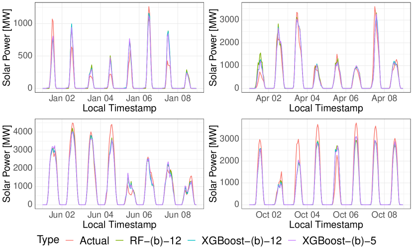
Figure 10: ASG forecasts for XGBoost-(b)-5, XGBoost-(b)-12, and RF-(b)-12 in 4 weeks during 2022 of the test set.

Figure 11 visualizes the daily RMSE and SMAPE performance of the top three configurations over the test set against the most simple configuration LR-(a)-average, whereas Figure 12 displays their cumulative sums. From the RMSE and SMAPE plots in Figure 11, we can clearly see that the linear model displays poor forecast performance with substantially higher peaks in the forecast errors particularly during the period from April to September. The cumulative plots in Figure 12 reveal that the LR model initially performs similarly to the more complex model configurations until the end of May 2022 but thereafter starts to deteriorate considerably compared to the top configurations. The top performing configurations all produce lower relative errors in the summer months when solar radiation is high and suffer from higher relative errors in the months from January to March and October to December when solar radiation decreases, see the SMAPE plot in Figure 11. All three top configurations closely track each other throughout the whole test period as can be seen from Figure 12 .

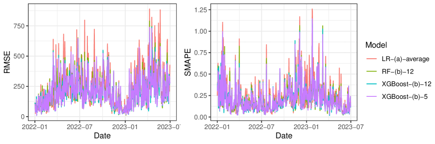
Figure 11: Daily RMSE (left) and daily SMAPE (right) plotted over the test-set for the configurations LR-(a)-average, XGBoost-(b)-5, XGBoost-(b)-12, and RF-(b)-12.

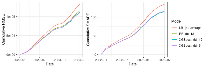
Figure 12: Cumulative daily RMSE (left) and daily SMAPE (right) plotted over the test-set for the configurations LR-(a)-average, XGBoost-(b)-5, XGBoost-(b)-12, and RF-(b)-12.

The cumulative plots in Figure 12 are also beneficial for detecting days or periods in which the model performs poorly compared to other periods. For instance, the performance of the top configurations during approximately the second half of March is very noisy with some inaccurate forecasts compared to the other forecasts in the test set. The slope of the cumulative plots during this period is indeed less smooth and some jumps can be observed. According to the national meteorological institution of Belgium responsible for monitoring and forecasting weather conditions, climate research, and providing meteorological services to the public and various sectors in Belgium (Koninglijk Meteorologisch Instituut van België,, 2022), this result could be attributed to extremely cold and cloudy days at the end of March and the beginning of April, which deviated from the expected weather patterns for that time of the season. Additionally, as shown in Figure 12, a single jump can be seen on April 1st, 2022. Koninglijk Meteorologisch Instituut van België, (2022) provides insightful information regarding the atypical performance of the models in this day since snowfall was recorded in multiple areas of Belgium, and this day was the coldest April 1st since the beginning of the measurements in 1901 thereby explaining why the forecast of ASG was considerably above the actual value. If one were to zoom into Figure 12, also July 21, 2022 and September 14, 2022, stand out as an atypical observations for a similar reason. Indeed, Koninglijk Meteorologisch Instituut van België, (2022) reveals the former as the cloudiest day of July with the lowest amount of radiation and the second rainiest day of the month. Similarly, September 14, 2022, was documented to be the cloudiest day of the month with the least solar radiation, thereby explaining the atypical performance of the models on this day. Given the exceptional nature of these three days, we classified them as outliers and excluded them from the tuning and training process to enhance model accuracy. However, they have been retained in the test set to evaluate the model’s performance under atypical weather conditions.

A final important aspect to consider when comparing the top model configurations concerns computing time. Data science practitioners are nowadays increasingly challenged on their carbon footprints due to the running of computationally intense algorithms. Overall, the XGBoost models are less computationally complex than the RF model: for instance, training the best configuration XGBoost-(b)-12 and the configuration XGBoost-(b)-5 on the combined training and validation datasets takes approximately 2 minutes and 42 seconds, respectively, whereas the RF-(b)-12 model configuration has a training time of 11 minutes. These time differences further support the preference for choosing the XGBoost configurations over the RF-based model configuration as the former combine the best forecast accuracy with a substantial reduction in computational cost.

5.2 Feature Importance

In this section, we investigate which parts of the information set in the top model configurations generate predictability. To this end, we conduct a feature importance study based on SHAP values (Lundberg and Lee,, 2017). SHAP (SHapley Additive exPlanation) values are considered to be the current state-of-the-art method for interpreting ML models, as they offer a unified framework for comparing feature importance across different ML models. SHAP values are based on the principles of cooperative game theory (Shapley,, 1953) where the Shapley value is a unique solution under certain properties to a coalitional game in which the goal is to distribute the worth of a grand coalition among players in a fair way. In the context of explaining ML model forecasts, the forecasts form the pay-off and the predictors are the individual players. The SHAP value for the $k$th feature at time point $t$ represents the feature’s contribution to the forecast at that time point, as measured in terms of the deviation from the response mean over the training sample. A variable importance score for each feature can then be obtained by summing the absolute SHAP values over all desired time points. We refer the interested reader to Molnar, (2020) for a detailed introduction to SHAP values.

To compute SHAP values for the RF and XGBoost models, we use the vip package (Greenwell and Boehmke,, 2020), which offers a fast implementation for tree-based ML models (Lundberg et al.,, 2020). Since each model is retrained every day, feature importance can change from day to day. To get an overall view of the SHAP values over the test set period, we calculate the SHAP values at the end of each month based on the forecast of the next month. Since our test set contains 18 months, the SHAP values are calculated 18 times. For each individual feature, we then compute its overall importance by taking the mean over all months of the test set. We subsequently analyze variable importance for each (i) location in the spatial grid, by summing feature importance over all meteorological variables at the particular location, (ii) meteorological feature, by computing the mean over all considered locations, and finally each (iii) feature-location combination at the most granular level.

Location Importance.

Figure 13 visualizes the contribution of each location to the overall forecasts for the two top performing model configurations RF and XGBoost with feature set (b) and 12 locations. Additionally, the Installed Capacity (IC) data of the provinces in Belgium, obtained from Elia Group Belgium., nd , is indicated by the red shading in Figure 13. Figure 13(a) for XGBoost shows that the locations around the latitude of $51^{\circ}$N are most important. These locations correspond to the northern provinces of Belgium where the IC is substantially higher than in the southern provinces. The most important locations at coordinates $4.25^{\circ}$E, $51^{\circ}$N and $5.25^{\circ}$E, $51.25^{\circ}$N are roughly located in the two regions with the highest IC. These findings therefore add to the validity of the feature importance study.

Figures 13(b) visualize the spatial importance for the RF model. Overall, a similar conclusion can be drawn as for the XGBoost model, but the discrepancies between the locations are larger for the RF model. Indeed, while the location at $4.25^{\circ}$E, $51^{\circ}$N is the most important one in both the XGBoost and RF models, the XGBoost model distributes considerably more weight among other locations, particularly western grid points at the latitude of $51^{\circ}$N, compared to the RF model.

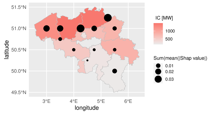
(a) XGBoost-(b)-12 clusters

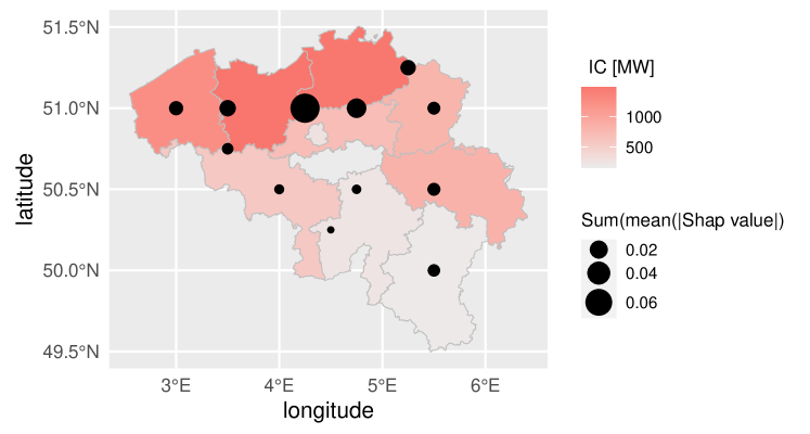
(b) RF-(b)-12 clusters

Figure 13: Location importance for the configurations with 12 clusters and feature set (b).

Meteorological and Astronomical Feature Importance.

Figure 14 summarizes the meteorological and astronomical feature importance of the RF and XGBoost models with feature set (b) across 12 locations. The SHAP results for XGBoost indicate that SNR is the most important for forecasting ASG, followed by Azimuth, Zenith, and RH, respectively. RF shows a slightly different feature importance where SNR is followed by Zenith, Azimuth and SSD. Hence, in line with the solar engineering literature (Duffie et al.,, 2020; Masters,, 2013), features directly related to solar energy have largest impact on day-ahead ASG forecasts. It is noticeable that Zenith and Azimuth display a similar feature importance in the XGBoost model configuration, whereas their importance differs substantially in the RF model configuration. The least important features are TCC, WCI, and T2m.

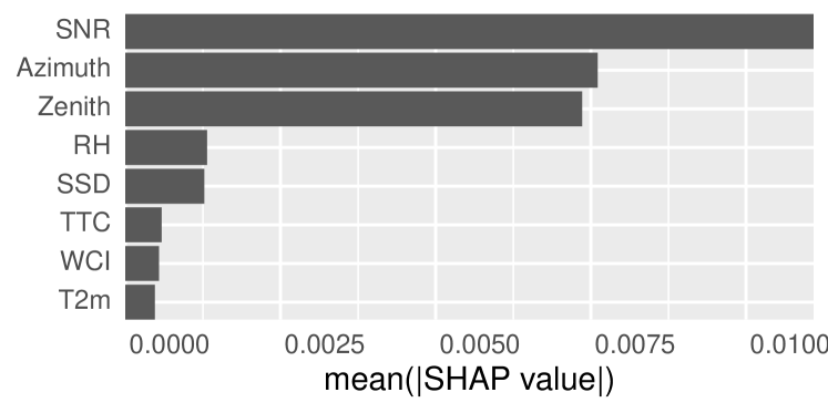
(a) XGBoost-(b)-12 clusters

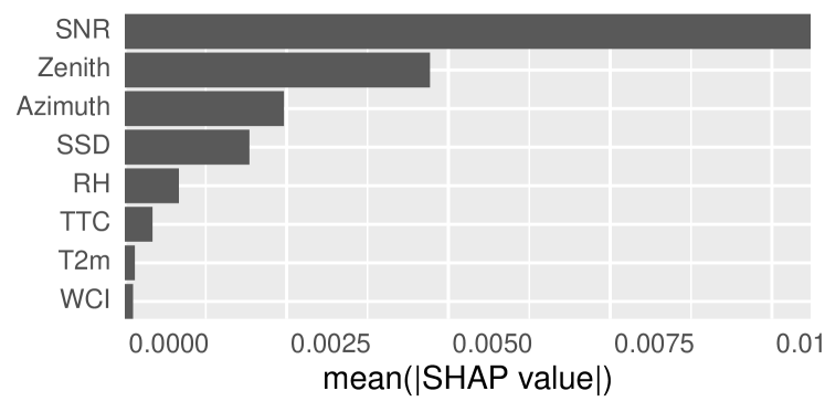
(b) RF-(b)-12 clusters

Figure 14: Feature importance for the configurations with 12 clusters and feature set (b).

Feature-Location Specific Importance.

Figure 15 illustrates the specific feature contributions at each spatial location. Note that Zenith and Azimuth are not included in this spatial analysis, as they are measured at a single location in Belgium. The main insights from the location and feature importance study are also reflected in the heatmaps of Figure 15. The location at coordinate $4.25^{\circ}$E, $51^{\circ}$N is by far the most important one, especially with respect to SNR and SSD. The heatmaps further reveal that XGBoost distributes the SHAP values more evenly among all features than the RF model does, thereby indicating that XGBoost utilizes a broader range of features to explain ASG.

In summary, our feature importance study clearly reveals the need to include location-specific meteorological information in the ML model to achieve accurate forecast performance. A fine-grained spatial feature importance study hereby helps to identify key locations, which, in turn, may be useful to to evaluate the potential importance of specific sites (Heo et al.,, 2021).

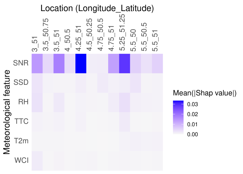
(a) XGBoost-(b)-12 clusters

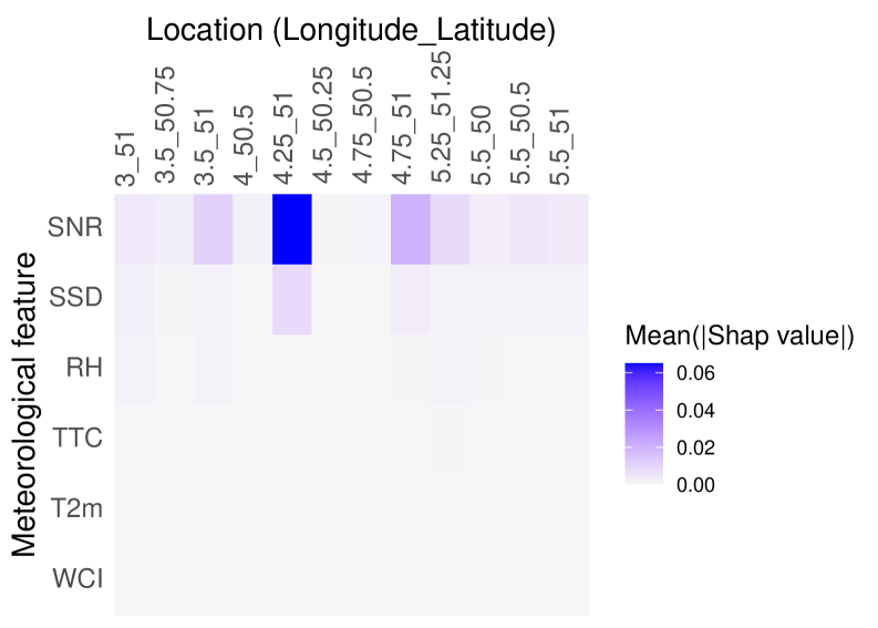
(b) RF-(b)-12 clusters

Figure 15: Specific feature importance for configurations with 12 clusters and feature set (b).

6 Conclusion

Due to the increased competition on the energy market and rise of technological advances such as digital meters, it becomes important for electricity providers and generators to correctly manage financial risks through models that capture electricity market dynamics at a granular level, as it would allow them to move towards a risk-based approach of pricing electricity contracts. This paper hereby focuses on forecasting short-term solar photovoltaic (PV) power, the second-fastest growing renewable energy source due to the increased penetration of PV energy into the electricity grid.

We put forward a comprehensive framework for forecasting day-ahead PV power generation using tree-based machine learning (ML) methods. The framework hereby accounts for possibly non-linear effects and the differential predictive power that various meteorological and astronomical features at fine-grained spatial locations have for (country-) aggregated Actual Solar Generation (ASG). Employing such a granular meteorology-informed PV power forecast model is crucial for grid management, economic dispatch optimization, clean energy technology, day-ahead electricity market trading, and facilitating the integration of distributed PV power into local electricity grids.

Our application for Belgian ASG reveals that an ensemble-based ML method like XGBoost is key to obtain accurate forecasts. The XGBoost model performs best when a diverse set of meteorological and astronomical features– whose relevance is supported by the solar engineering, photovoltaic systems and meteorology literature –measured at a fine-grained spatial resolution are included in the forecaster’s information set. To gain insights into the forecast capabilities of various model configuration, we offer practitioners a diverse set of visualizations one can use to track forecast performance across time, and to reveal feature importance through SHAP values and this at a coarse (location or feature-based) as well as at a fine-grained level (for location-specific features).

Several directions for future research emerge. We focus on solar-based energy, but the proposed forecasting framework could equally well be applied to model day-ahead wind energy output. Furthermore, we focus on point forecasts but probabilistic forecasts could provide crucial additional information enabling decision-makers to assess risks and investments associated with resource allocation, grid stability, day-ahead trading, and other fields of PV power forecasting (Juban et al.,, 2008). To this end, the quantile regression forest approach of Bellinguer et al., (2020) or the XGBoost extension by März, (2019) offering forecast intervals and quantiles are interesting avenues to further explore.

Finally, while we focus on a short-term (day-ahead) forecast horizon, the ML models all use fundamental driving factors of solar generation, selected based on a careful investigation of the meteorological literature, in the forecaster’s information set. This opens up the door for future research into a holistic modeling approach between short-term and long-term models for electricity prices which crucially rely on expectations of renewable production and are essential for electricity providers to assess their risk exposure. To this end, it will be vital to investigate in future research how one can incorporate uncertainty regarding these fundamental drivers through scenario building (see e.g., Müller et al.,, 2015 for gas), and to robustify the forecasting framework to downweight the influence of atypical data values in order to capture stable/robust long-term dynamics (Leoni et al.,, 2018).

References

- Abdurrahman et al., (2019) Abdurrahman, M., Gambo, J., Shitu, I., Yusuf, Y., Dahiru, Z., Idris, A., and Isah, A. (2019). Solar elevation angle and solar culmination determination using celestial observation; a case study of hadejia jigawa state, nigeria. International Journal of Advance in Scientific Research and Engineering, 5(9):08–17.
- (2) Abuella, M. and Chowdhury, B. (2015a). Solar power forecasting using artificial neural networks. In 2015 North American Power Symposium (NAPS), pages 1–5. IEEE.
- (3) Abuella, M. and Chowdhury, B. (2015b). Solar power probabilistic forecasting by using multiple linear regression analysis. In SoutheastCon 2015, pages 1–5. IEEE.
- Alkabbani et al., (2021) Alkabbani, H., Ahmadian, A., Zhu, Q., and Elkamel, A. (2021). Machine learning and metaheuristic methods for renewable power forecasting: A recent review. Frontiers in Chemical Engineering, 3:665415.
- Amajama and Mopta, (2016) Amajama, J. and Mopta, S. (2016). Effect of air temperature on the output of photovoltaic panels and its relationship with solar illuminance/intensity. International Journal of Scientific Engineering and Applied Science (IJSEAS), 2:161–166.
- Amajama and Oku, (2016) Amajama, J. and Oku, D. (2016). Effect of relative humidity on photovoltaic panels’ output and solar illuminance/intensity. 2016:126–130.
- Antonanzas et al., (2016) Antonanzas, J., Osorio, N., Escobar, R., Urraca, R., de Pison, F. M., and Antonanzas-Torres, F. (2016). Review of photovoltaic power forecasting. Solar Energy, 136:78–111.
- Baños et al., (2011) Baños, R., Manzano-Agugliaro, F., Montoya, F., Gil, C., Alcayde, A., and Gómez, J. (2011). Optimization methods applied to renewable and sustainable energy: A review. Renewable and Sustainable Energy Reviews, 15(4):1753–1766.
- Bellinguer et al., (2020) Bellinguer, K., Mahler, V., Camal, S., and Kariniotakis, G. (2020). Probabilistic forecasting of regional wind power generation for the EEM20 competition: a physics-oriented machine learning approach. In 17th European Energy Market Conference, EEM 2020, Stockholm (by visio), Sweden. KTH, IEEE.
- Bernardi, (2017) Bernardi, L. C. . M. (2017). MCS: Model Confidence Set Procedure. R package version 0.1.3.
- Breiman, (1984) Breiman, L. (1984). Classification And Regression Trees. Routledge.
- Breiman, (2001) Breiman, L. (2001). Random forests. Machine Learning, 45:5–32.
- Chen and Guestrin, (2016) Chen, T. and Guestrin, C. (2016). Xgboost: A scalable tree boosting system. In Proceedings of the 22nd acm sigkdd international conference on knowledge discovery and data mining, pages 785–794.
- Chen et al., (2023) Chen, T., He, T., Benesty, M., Khotilovich, V., Tang, Y., Cho, H., Chen, K., Mitchell, R., Cano, I., Zhou, T., Li, M., Xie, J., Lin, M., Geng, Y., Li, Y., and Yuan, J. (2023). xgboost: Extreme Gradient Boosting. R package version 1.7.5.1.
- Copernicus Climate Change Service, Climate Data Store, (2023) Copernicus Climate Change Service, Climate Data Store (2023). ERA5 hourly data on single levels from 1940 to present. Copernicus Climate Change Service (C3S) Climate Data Store (CDS). DOI: 10.24381/cds.adbb2d47.
- Duffie et al., (2020) Duffie, J. A., Beckman, W. A., and Blair, N. (2020). Solar engineering of thermal processes, photovoltaics and wind. John Wiley & Sons.
- (17) Elia Group Belgium (n.d.). Photovoltaic power production estimation and forecast on Belgian grid (Historical).
- (18) Elia Group Belgium. (n.d.). Solar PV Power Generation Data. URL: https://www.elia.be/en/grid-data/power-generation/solar-pv-power-generation-data?csrt=9425284229408774527.
- Friedman, (2001) Friedman, J. H. (2001). Greedy function approximation: A gradient boosting machine. The Annals of Statistics, 29(5):1189–1232.
- Greenwell and Boehmke, (2020) Greenwell, B. M. and Boehmke, B. C. (2020). Variable importance plots—an introduction to the vip package. The R Journal, 12(1):343–366.
- Han et al., (2019) Han, S., hui Qiao, Y., Yan, J., qian Liu, Y., Li, L., and Wang, Z. (2019). Mid-to-long term wind and photovoltaic power generation prediction based on copula function and long short term memory network. Applied Energy, 239:181–191.
- Hansen et al., (2011) Hansen, P., Lunde, A., and Nason, J. (2011). The model confidence set. Econometrica, 79(2):453–497.
- Hastie et al., (2009) Hastie, T., Tibshirani, R., and Friedman, J. (2009). The elements of statistical learning: data mining, inference and prediction. Springer, 2 edition.
- Hegde et al., (2016) Hegde, V., Aswathi, T. S., and Sidharth, R. (2016). Student residential distance calculation using haversine formulation and visualization through googlemap for admission analysis. 2016 IEEE International Conference on Computational Intelligence and Computing Research (ICCIC), pages 1–5.
- Heo et al., (2021) Heo, J., Song, K., Han, S., and Lee, D.-E. (2021). Multi-channel convolutional neural network for integration of meteorological and geographical features in solar power forecasting. Applied Energy, 295:117083.
- Hersbach et al., (2023) Hersbach, H., Bell, B., Berrisford, P., Biavati, G., Horányi, A., Sabater, J., Nicolas, J., Peubey, C., Radu, R., Rozum, I., Schepers, D., Simmons, A., Soci, C., Dee, D., and Thépaut, J.-N. (2023). ERA5 hourly data on single levels from 1940 to present. Copernicus Climate Change Service (C3S) Climate Data Store (CDS). DOI: 10.24381/cds.adbb2d47.
- Inman et al., (2013) Inman, R. H., Pedro, H. T., and Coimbra, C. F. (2013). Solar forecasting methods for renewable energy integration. Progress in Energy and Combustion Science, 39(6):535–576.
- Jacobson et al., (2019) Jacobson, M., Delucchi, M., Cameron, M., Coughlin, S., Callas, C., Manogaran, I., Shu, Y., and von Krauland, A.-K. (2019). Impacts of green new deal energy plans on grid stability, costs, jobs, health, and climate in 143 countries. One Earth, 1:449–463.
- Januschowski et al., (2022) Januschowski, T., Wang, Y., Torkkola, K., Erkkilä, T., Hasson, H., and Gasthaus, J. (2022). Forecasting with trees. International Journal of Forecasting, 38(4):1473–1481.
- Juban et al., (2008) Juban, J., Fugon, L., and Kariniotakis, G. (2008). Uncertainty estimation of wind power forecasts: Comparison of probabilistic modelling approaches. In European Wind Energy Conference & Exhibition EWEC 2008, pages 10–pages. EWEC.
- Kaushaley et al., (2023) Kaushaley, S., Shaw, B., and Nayak, J. R. (2023). Optimized machine learning-based forecasting model for solar power generation by using crow search algorithm and seagull optimization algorithm. Arabian Journal for Science and Engineering, pages 1–14.
- Koninglijk Meteorologisch Instituut van België, (2022) Koninglijk Meteorologisch Instituut van België (2022). Klimatologische overzichten van 2022. https://www.meteo.be/nl/klimaat/klimaat-van-belgie/klimatologisch-overzicht/2022/april.
- Krishnan et al., (2023) Krishnan, N., Kumar, K. R., and Inda, C. S. (2023). How solar radiation forecasting impacts the utilization of solar energy: A critical review. Journal of Cleaner Production, 388:135860.
- Lankford and Fox, (2021) Lankford, H. V. and Fox, L. R. (2021). The wind-chill index. Wilderness & Environmental Medicine, 32(3):392–399.
- Leoni et al., (2018) Leoni, P., Segaert, P., Serneels, S., and Verdonck, T. (2018). Multivariate constrained robust m-regression for shaping forward curves in electricity markets. Journal of Futures Markets, 38(11):1391–1406.
- Leva et al., (2017) Leva, S., Dolara, A., Grimaccia, F., Mussetta, M., and Ogliari, E. (2017). Analysis and validation of 24 hours ahead neural network forecasting of photovoltaic output power. Mathematics and Computers in Simulation, 131:88–100. 11th International Conference on Modeling and Simulation of Electric Machines, Converters and Systems.
- Liu et al., (2020) Liu, Z.-F., Li, L.-L., Tseng, M.-L., and Lim, M. K. (2020). Prediction short-term photovoltaic power using improved chicken swarm optimizer - extreme learning machine model. Journal of Cleaner Production, 248:119272.
- Lundberg and Lee, (2017) Lundberg, S. and Lee, S.-I. (2017). A unified approach to interpreting model predictions.
- Lundberg et al., (2020) Lundberg, S. M., Erion, G., Chen, H., DeGrave, A., Prutkin, J. M., Nair, B., Katz, R., Himmelfarb, J., Bansal, N., and Lee, S.-I. (2020). From local explanations to global understanding with explainable ai for trees. Nature machine intelligence, 2(1):56–67.
- März, (2019) März, A. (2019). Xgboostlss–an extension of xgboost to probabilistic forecasting. arXiv preprint arXiv:1907.03178.
- Masters, (2013) Masters, G. M. (2013). Renewable and efficient electric power systems. John Wiley & Sons.
- Meral and Dinçer, (2011) Meral, M. E. and Dinçer, F. (2011). A review of the factors affecting operation and efficiency of photovoltaic based electricity generation systems. Renewable and Sustainable Energy Reviews, 15(5):2176–2184.
- Molnar, (2020) Molnar, C. (2020). Interpretable machine learning: A guide for making black box models explainable. Creative Common License.
- Müller et al., (2015) Müller, J., Hirsch, G., and Müller, A. (2015). Modeling the price of natural gas with temperature and oil price as exogenous factors. In Innovations in Quantitative Risk Management: TU München, September 2013, pages 109–128. Springer International Publishing.
- Ouikhalfan et al., (2022) Ouikhalfan, M., Lakbita, O., Delhali, A., Assen, A. H., and Belmabkhout, Y. (2022). Toward net-zero emission fertilizers industry: Greenhouse gas emission analyses and decarbonization solutions. Energy & Fuels, 36(8):4198–4223.
- Our World in Data, (2023) Our World in Data (2023). Installed solar pv capacity. Accessed on 30-10-2023.
- Panjwani et al., (2017) Panjwani, M. K., Panjwani, S. K., Mangi, F. H., Khan, D., and Meicheng, L. (2017). Humid free efficient solar panel. In AIP Conference Proceedings, volume 1884. AIP Publishing.
- R Core Team, (2023) R Core Team (2023). R: A Language and Environment for Statistical Computing. R Foundation for Statistical Computing, Vienna, Austria.
- Reda and Andreas, (2004) Reda, I. and Andreas, A. (2004). Solar position algorithm for solar radiation applications. Solar Energy, 76(5):577–589.
- Santner et al., (2003) Santner, T., Williams, B., and Notz, W. (2003). The Design and Analysis Computer Experiments.
- Schwingshackl et al., (2013) Schwingshackl, C., Petitta, M., Wagner, J., Belluardo, G., Moser, D., Castelli, M., Zebisch, M., and Tetzlaff, A. (2013). Wind effect on pv module temperature: Analysis of different techniques for an accurate estimation. Energy Procedia, 40:77–86. European Geosciences Union General Assembly 2013, EGUDivision Energy, Resources & the Environment, ERE.
- Shapley, (1953) Shapley, L. S. (1953). 17. A Value for n-Person Games, pages 307–318. Princeton University Press, Princeton.
- Sharma et al., (2011) Sharma, N., Sharma, P., Irwin, D., and Shenoy, P. (2011). Predicting solar generation from weather forecasts using machine learning. In 2011 IEEE International Conference on Smart Grid Communications (SmartGridComm), pages 528–533.
- Son and Jung, (2020) Son, N. and Jung, M. (2020). Analysis of meteorological factor multivariate models for medium- and long-term photovoltaic solar power forecasting using long short-term memory. Applied Sciences, 11:316.
- Sudharshan et al., (2022) Sudharshan, K., Naveen, C., Vishnuram, P., Krishna Rao Kasagani, D. V. S., and Nastasi, B. (2022). Systematic review on impact of different irradiance forecasting techniques for solar energy prediction. Energies, 15(17).
- Tang et al., (2018) Tang, N., Mao, S., Wang, Y., and Nelms, R. M. (2018). Solar power generation forecasting with a lasso-based approach. IEEE Internet of Things Journal, 5(2):1090–1099.
- Therneau and Atkinson, (2022) Therneau, T. and Atkinson, B. (2022). rpart: Recursive Partitioning and Regression Trees. R package version 4.1.19.
- Van doninck, (2016) Van doninck, J. (2016). solarPos: Solar Position Algorithm for Solar Radiation Applications. R package version 1.0.
- Visser et al., (2019) Visser, L., AlSkaif, T., and Sark, W. v. (2019). Benchmark analysis of day-ahead solar power forecasting techniques using weather predictions. In 2019 IEEE 46th Photovoltaic Specialists Conference (PVSC), pages 2111–2116.
- Vokrouhlickỳ and Sehnal, (1993) Vokrouhlickỳ, D. and Sehnal, L. (1993). Cloud coverage aspects of the albedo effect. Celestial Mechanics and Dynamical Astronomy, 57:493–508.
- Voyant et al., (2017) Voyant, C., Notton, G., Kalogirou, S., Nivet, M.-L., Paoli, C., Motte, F., and Fouilloy, A. (2017). Machine learning methods for solar radiation forecasting: A review. Renewable Energy, 105:569–582.
- Wan et al., (2015) Wan, C., Zhao, J., Song, Y., Xu, Z., Lin, J., and Hu, Z. (2015). Photovoltaic and solar power forecasting for smart grid energy management. CSEE Journal of Power and Energy Systems, 1(4):38–46.
- Weron, (2014) Weron, R. (2014). Electricity price forecasting: A review of the state-of-the-art with a look into the future. International Journal of Forecasting, 30(4):1030–1081.
- Wolniak and Skotnicka-Zasadzien, (2022) Wolniak, R. and Skotnicka-Zasadzien, B. (2022). Development of photovoltaic energy in EU countries as an alternative to fossil fuels. Energies, 15:662.
- Wright and Ziegler, (2017) Wright, M. N. and Ziegler, A. (2017). ranger: A fast implementation of random forests for high dimensional data in C++ and R. Journal of Statistical Software, 77(1):1–17.
- Xydis, (2013) Xydis, G. (2013). The wind chill temperature effect on a large-scale pv plant—an exergy approach. Progress in Photovoltaics: Research and Applications, 21(8):1611–1624.
- Yu and Hong, (2016) Yu, M. and Hong, S. H. (2016). Supply–demand balancing for power management in smart grid: A stackelberg game approach. Applied Energy, 164:702–710.
- Zamo et al., (2014) Zamo, M., Mestre, O., Arbogast, P., and Pannekoucke, O. (2014). A benchmark of statistical regression methods for short-term forecasting of photovoltaic electricity production, part i: Deterministic forecast of hourly production. Solar Energy, 105:792–803.
- Zeng and Qiao, (2013) Zeng, J. and Qiao, W. (2013). Short-term solar power prediction using a support vector machine. Renewable Energy, 52:118–127.
- Zhang et al., (2015) Zhang, J., Florita, A., Hodge, B.-M., Lu, S., Hamann, H. F., Banunarayanan, V., and Brockway, A. M. (2015). A suite of metrics for assessing the performance of solar power forecasting. Solar Energy, 111:157–175.
- Zsiborács et al., (2021) Zsiborács, H., Pintér, G., Vincze, A., Birkner, Z., and Baranyai, N. H. (2021). Grid balancing challenges illustrated by two european examples: Interactions of electric grids, photovoltaic power generation, energy storage and power generation forecasting. Energy Reports, 7:3805–3818.