A constructive approach for investigating the stability of incommensurate fractional differential systems

Abstract

This paper is devoted to studying the asymptotic behaviour of solutions to generalized non-commensurate fractional systems. To this end, we first consider fractional systems with rational orders and introduce a criterion that is necessary and sufficient to ensure the stability of such systems. Next, from the fractional-order pseudospectrum definition proposed by Šanca et al., we formulate the concept of a rational approximation for the fractional spectrum of a noncommensurate fractional systems with general, not necessarily rational, orders. Our first important new contribution is to show the equivalence between the fractional spectrum of a noncommensurate linear system and its rational approximation. With this result in hand, we use ideas developed in our earlier work to demonstrate the stability of an equilibrium point to nonlinear systems in arbitrary finite-dimensional spaces. A second novel aspect of our work is the fact that the approach is constructive. Finally, we give numerical simulations to illustrate the merit of the proposed theoretical results.

Key words: Fractional differential equations, non-commensurate fractional systems, fractional spectrum, fractional-order pseudospectrum, Mittag-Leffler stability

AMS subject classifications: Primary 34A08, 34D20; Secondary 26A33, 34C11, 45A05, 45D05, 45M05, 45M10

1 Introduction

The primary goal of this work is to establish a deeper understanding of the stability of non-commensurate systems of fractional differential equations with Caputo operators. To the best of our knowledge, the first paper to investigate such questions was [2] where it was shown that the system is stable if the zeros of its fractional characteristic polynomial are in the open left half of the complex plane. While this result is very valuable from a theoretical point of view, it is only of rather limited practical use because finding roots of a fractional characteristic polynomial of a non-commensurate fractional-order system is a complicated task that has so far only been solved in some special cases.

Our aim in this paper is to propose a comprehensive, complete approach to solving the aforementioned problem. Our approach follows. First, we consider fractional-order systems with rational orders and give a necessary and sufficient condition for their stability. Then we study general fractional-order systems with arbitrary (rational or irrational) orders. Inspired by ideas in [12], we construct rational approximations of the fractional spectrum of a matrix. The existence of these approximations is verified. Furthermore, we demonstrate the equivalence of the fractional spectrum of a matrix and its rational approximation. From this we bring the problem under investigation to the case when the fractional orders are rational which we already know how to solve clearly. The peculiarity of our approach is constructiveness. Based on the strategies that we propose, it is not difficult to build computer programs to check the stability of any fractional-order system.

The rest of the article is organized as follows. In Section 2, we introduce the definitions of fractional derivatives, fractional spectra and pseudo-spectra, and some notations that will be used throughout the paper. In Section 3, we prove a necessary and sufficient criterion for the stability of multi-order fractional systems with rational orders. Section 4 deals with generalized fractional order systems (systems containing many different, not necessarily rational, fractional derivatives). This section contains the main results that are our most important contributions to understanding and solving the problem at hand. Next, the Mittag-Leffler stability of an equilibrium point of non-commensurate fractional nonlinear systems is presented in Section 5. Finally, numerical simulations are given in Section 6 to illustrate the obtained theoretical results.

2 Preliminaries

For $\alpha\in(0,1]$ and $J=[0,T]$ or $J=[0,\infty)$, the Riemann-Liouville fractional integral of a function $f:J\rightarrow\mathbb{R}$ is defined by

$$I^{\alpha}_{0^{+}}x(t):=\frac{1}{\Gamma(\alpha)}\int_{0}^{t}(t-s)^{\alpha-1}x(s)\,{\mathrm{d}}s,\ \quad t\in J,$$

and its Caputo fractional derivative of the order $\alpha\in(0,1)$ as

$${}^{C}D^{\alpha}_{0^{+}}x(t):=\frac{{\mathrm{d}}}{{\mathrm{d}}t}I^{1-\alpha}_{0^{+}}(f(t)-f(0)),\quad t\in J\setminus\{0\},$$

where $\Gamma(\cdot)$ is the Gamma function and $\frac{{\mathrm{d}}}{{\mathrm{d}}t}$ is the classical derivative; see. e.g., [3, Chapters 2 and 3] or [1]. Let $n\in\mathbb{N}$, $\hat{\alpha}=(\alpha_{1},\alpha_{2},\ldots,\alpha_{n})\in(0,1]^{n}$ be a multi-index and $x=(x_{1},\ldots,x_{n})^{\rm T}$ with $x_{i}:J\rightarrow\mathbb{R}$, $i=1,\ldots,n$, be a vector valued function. Then we denote

$${}^{C}D^{\hat{\alpha}}_{0^{+}}x(t):=\left({}^{C}D^{\alpha_{1}}_{0^{+}}x_{1}(t),\ldots,{}^{C}D^{\alpha_{n}}_{0^{+}}x_{n}(t)\right)^{\mathrm{T}}.$$

For each $n\in\mathbb{N}$, we denote the set of complex square matrices of order $n$ by $M_{n}(\mathbb{C})$, and $M_{n}(\mathbb{R})\subset M_{n}(\mathbb{C})$ is the set of real square matrices of order $n$. The unit matrix of order $n$ is denoted by $I$. For a given matrix $A=(a_{ij})_{n\times n}\in M_{n}(\mathbb{C})$, we use $A^{\mathrm{T}}=(a_{ji})_{n\times n}$ to denote its transpose matrix and $A^{*}=(\overline{a_{ji}})_{n\times n}$ is the conjugate transpose matrix. For any $B\in M_{n}(\mathbb{C})$, its spectrum is defined by $\sigma(B):=\{z\in\mathbb{C}:\det(zI-B)=0\}$. Furthermore, for each $z\in\mathbb{C}$, we put $z^{\hat{\alpha}}I:=\mathop{\mathrm{diag}}(z^{\alpha_{1}},\ldots,z^{\alpha_{n}})$. Here and in many places later on in the paper we encounter powers of complex numbers with noninteger exponents in the range $(0,1)$. Whenever such an expression occurs, we will interpret this in the sense of the principal branch of the (potentially multi-valued) complex power function, i.e. we say

$$z^{\beta}=|z|^{\beta}\exp({\mathrm{i}}\beta\arg(z))$$

whenever $\beta\in(0,1)$ and $z\in\mathbb{C}$.

Next, we recall some concepts of matrix norms and pseudospectra. To simplify the notation, we write $N=\{1,2,\ldots,n\}$. On $\mathbb{C}^{n}$, we select a (for the time being, arbitrary) norm $\|\cdot\|$. The associated matrix norm is also designated by $\|\cdot\|$. For convenience, we use the convention $\|M^{-1}\|^{-1}=0$ if and only if $\det M=0$. For each $x\in\mathbb{C}^{n}$, we set $\Re(x)=(\Re(x_{1}),\ldots,\Re(x_{n}))$. We denote the scalar product in $\mathbb{C}^{n}$ by $\left\langle\cdot\,,\cdot\right\rangle$ and set $\mathbb{C}_{-}:=\{z\in\mathbb{C}:\Re(z)<0\}$ and $\mathbb{C}_{\geq 0}:=\{z\in\mathbb{C}:\Re(z)\geq 0\}$.

From [12, p. 248], we now recall the essential concepts that we shall use to a large extent throughout this paper.

Definition 2.1.

Let $n\in\mathbb{N}$, $A\in M_{n}(\mathbb{R})$ and $\hat{\alpha}=(\alpha_{1},\ldots,\alpha_{n})\in(0,1]^{n}$. Then, the $\hat{\alpha}$-order spectrum of $A$ is the set

$$\sigma_{\hat{\alpha}}(A):=\left\{z\in\mathbb{C}:\det\left(\mathop{\mathrm{diag}}(z^{\alpha_{1}},\ldots,z^{\alpha_{n}})-A\right)=0\right\},$$

Moreover, for $\epsilon>0$, the $\hat{\alpha}$-order $\epsilon$-pseudospectrum of $A$ is defined by

$$\sigma_{\hat{\alpha},\epsilon}(A):=\{z\in\mathbb{C}:\|(z^{\hat{\alpha}}I-A)^{-1}\|^{-1}\leq\epsilon\}.$$ (1)

It is clear from the above definition that the $\hat{\alpha}$-order $\epsilon$-pseudospectrum depends on the used norm $\|\cdot\|$. Therefore, to indicate this dependence, we will use the notation $\sigma_{\hat{\alpha},\epsilon}^{p}(A)$ instead of $\sigma_{\hat{\alpha},\epsilon}(A)$ in the case where the norm $\|\cdot\|$ is specifically chosen as the norm $\|\cdot\|_{p}$ with some $1\leq p\leq\infty$. The $\hat{\alpha}$-order spectrum, on the other hand, clearly does not depend on the chosen norm and hence does not need such a notational clarification.

Proposition 2.2.

For some given $\epsilon>0$, $\hat{\alpha}\in(0,1]^{n}$ and $A\in M_{n}(\mathbb{R})$, the $\hat{\alpha}$-order $\epsilon$-pseudospectrum of $A$ can be expressed in the following ways:

$$\sigma_{\hat{\alpha},\epsilon}(A) =\{z\in\mathbb{C}:\exists E\in M_{n}(\mathbb{C}),\|E\|\leq\epsilon\;\text{such that}\,z\in\sigma_{\hat{\alpha}}(A+E)\}$$ (2)

$$=\{z\in\mathbb{C}:\exists v\in\mathbb{C}^{n},\|v\|=1\;\text{such that}\,\|(z^{\hat{\alpha}}I-A)v\|\leq\epsilon\}.$$ (3)

Proof.

See [12, Theorem 2.3, p. 249] or [14, Theorem 2.1, p. 16]. ∎

Theorem 2.3 ($\hat{\alpha}$-fractional $\epsilon$-pseudo Geršgorin sets).

Let $A\in M_{n}(\mathbb{R})$ and $\hat{\alpha}\in(0,1]^{n}$ and consider the norm $\|\cdot\|_{\infty}$. For any $\epsilon>0$, we have

$$\sigma_{\hat{\alpha},\epsilon}^{\infty}(A)\subset\bigcup_{i\in N}\left\{z\in\mathbb{C}:|a_{ii}-z^{\alpha_{i}}|\leq r_{i}(A)+\epsilon\right\}$$

where $r_{i}(A)=\sum_{j\in N,j\neq i}|a_{ij}|$.

Proof.

See [12, Theorem 3.1, p. 251]. ∎

Remark 2.4.

Taking the limit $\epsilon\to 0$, it follows from Definition 2.1 and Theorem 2.3 that

$$\sigma_{\hat{\alpha}}(A)\subset\bigcup_{i\in N}\left\{z\in\mathbb{C}:|a_{ii}-z^{\alpha_{i}}|\leq r_{i}(A)\right\}.$$

Thus, if $A$ is a diagonally dominant matrix with negative elements on the main diagonal, then $\sigma_{\hat{\alpha}}(A)\subset\mathbb{C}_{-}$ for all $\hat{\alpha}\in(0,1]^{n}$. As shown in [15], this implies that the associated linear differential equation system with orders $\hat{\alpha}$ and the constant coefficient matrix $A$ (as given in eq. (4) below) is asymptotically stable.

Due to the fact that all norms on $M_{n}(\mathbb{C})$ are equivalent, for specificity and convenience of presentation, from now on we will only state and prove the results for the norm $\|\cdot\|_{2}$.

Theorem 2.5 (Euclidean $\hat{\alpha}$-fractional $\epsilon$-pseudo Geršgorin sets).

For given $A\in M_{n}(\mathbb{R})$, $\hat{\alpha}\in(0,1]^{n}$ and $\epsilon>0$, we have

$$\sigma_{\hat{\alpha},\epsilon}^{2}(A)\subset\bigcup_{i\in N}\left\{z\in\mathbb{C}:|a_{ii}-z^{\alpha_{i}}|\leq\max\{r_{i}(A),r_{i}(A^{\mathrm{T}})\}+\epsilon\right\}$$

Proof.

See [12, Theorem 3.4, pp. 260]. ∎

Remark 2.6.

When applying Theorem 2.5, it is helpful to remember the immediately obvious relation $r_{i}(A^{\mathrm{T}})=\sum_{j\in N,j\neq i}|a_{ji}|$.

3 The $\hat{\alpha}$-order spectrum: The case $\hat{\alpha}\in\left((0,1]\cap\mathbb{Q}\right)^{n}$

Let $\hat{\alpha}=(\alpha_{1},\ldots\alpha_{n})\in(0,1]^{n}$. Then we initially consider the system

$$^{C}D^{\hat{\alpha}}_{0^{+}}x(t) =Ax(t),\quad t>0,$$ (4)

$$x(0) =x^{0}\in\mathbb{R}^{n},$$ (5)

with some $A\in M_{n}(\mathbb{R})$. Following [13], we shall first discuss our problem for the case that all orders $\alpha_{i}$ are rational numbers and defer the extension to irrational values of $\alpha_{i}$ until Section 4. Thus, in this section we assume that $\alpha_{i}\in\mathbb{Q}$ for all $i\in N$, and so we have $\alpha_{i}=\frac{q_{i}}{m_{i}}$ with some $q_{i},m_{i}\in\mathbb{N}$ (assumed to be in lowest terms) for all $i\in N$. Let $m$ be the least common multiple of $m_{1},\ldots,m_{n}$ and $\gamma=1/m\in(0,1]$. Then,

$$z^{\hat{\alpha}}I-A =\mathop{\mathrm{diag}}(z^{\alpha_{1}},\ldots,z^{\alpha_{n}})-A$$

$$=\mathop{\mathrm{diag}}(z^{\frac{q_{1}}{m_{1}}},\ldots,z^{\frac{q_{n}}{m_{n}}})-A$$

$$=\mathop{\mathrm{diag}}(z^{\frac{p_{1}}{m}},\ldots,z^{\frac{p_{n}}{m}})-A$$

$$=\mathop{\mathrm{diag}}((z^{\gamma})^{p_{1}},\ldots,(z^{\gamma})^{p_{n}})-A$$

where $p_{i}=q_{i}\frac{m}{m_{i}}\in\mathbb{N}$ for $i=1,2,\ldots,n$. Writing $s=z^{\gamma}$, we obtain

$$\det(z^{\hat{\alpha}}I-A)=\det(s^{\hat{p}}I-A)$$ (6)

where $\hat{p}=(p_{1},\ldots,p_{n})^{\rm T}\in\mathbb{N}^{n}$.

Since $s=z^{\gamma}$ in eq. (6), it is clear that $\arg(s)\in(-\gamma\pi,\gamma\pi]$. Therefore, to analyze the zeros of the expression on the right-hand side of eq. (6), it is necessary to discuss the set

$$\tilde{\sigma}_{\hat{p}}^{(\gamma)}(A)=\{s\in\mathbb{C}:\arg(s)\in(-\gamma\pi,\gamma\pi]\text{ and }\det(s^{\hat{p}}I-A)=0\}.$$ (7)

In this context, we then see that we have $\sigma_{\hat{\alpha}}(A)\subset\mathbb{C}_{-}$ if and only if $\tilde{\sigma}_{\hat{p}}^{(\gamma)}(A)\in\Omega_{\gamma}$ where

$$\Omega_{\gamma}=\left\{z\in\mathbb{C}\setminus\{0\}:|\arg(z)|>\gamma\frac{\pi}{2},-\gamma\pi<\arg(z)\leq\gamma\pi\right\}.$$ (8)

In view of eq. (7), it is thus of interest to compute $\det(s^{\hat{p}}I-A)$. First of all, for each set $\{i_{1},i_{2},\ldots,i_{r}\}$ with $1\leq i_{1}<\ldots<i_{r}\leq n$ and $1\leq r\leq n$, we will determine the coefficient of each monomial $s^{p_{i_{1}}}\cdots s^{p_{i_{r}}}$ in the expansion of $\det(s^{\hat{p}}I-A)$. Note that in this expansion we will treat $p_{1},p_{2},\ldots,p_{n}$ as formal variables, i.e., $s^{p_{i}}s^{p_{j}}\neq s^{p_{j}}s^{p_{i}}$ with every $i\neq j$. We then have

$$\det(s^{\hat{p}}I-A) =\det\begin{pmatrix}s^{p_{1}}-a_{11}&-a_{12}&\ldots&-a_{1n}\\ -a_{21}&s^{p_{2}}-a_{22}&\ldots&-a_{2n}\\ \vdots&\vdots&\ddots&\vdots\\ -a_{n1}&-a_{n2}&\ldots&s^{p_{n}}-a_{nn}\\ \end{pmatrix}$$

$$=s^{p_{i_{1}}}\Delta^{A}_{(i_{1};i_{1})}-\sum_{j=1}^{n}(-1)^{i_{1}+j}a_{i_{1}j}\Delta^{A}_{(i_{1};j)},$$

where $\Delta^{A}_{(i_{1};j)}$, $j\in N$, is the determinant of the matrix obtained from $s^{\hat{p}}I-A$ by removing the $i_{1}$-th row and the $j$-th column. It is easy to see that the term $s^{p_{i_{1}}}\cdots s^{p_{i_{r}}}$ only appears in $s^{p_{i_{1}}}\Delta^{A}_{(i_{1};i_{1})}$. Therefore, the coefficient of $s^{p_{i_{1}}}\cdots s^{p_{i_{r}}}$ in the expansion $s^{\hat{p}}I-A$ is equal to the coefficient of $s^{p_{i_{1}}}\cdots s^{p_{i_{r}}}$ in the expansion of $s^{p_{i_{1}}}\Delta^{A}_{(i_{1};i_{1})}$. Moreover,

$$s^{p_{i_{1}}}\Delta^{A}_{(i_{1};i_{1})} =s^{p_{i_{1}}}s^{p_{i_{2}}}\Delta^{A}_{(i_{1},i_{2};i_{1},i_{2})}-\sum_{j\in N,j\neq i_{1}}(-1)^{i_{2}+j}a_{i_{2}j}\Delta^{A}_{(i_{1},i_{2};i_{1},j)}$$

with $\Delta^{A}_{(i_{1},i_{2};i_{1},j)}$, $j\in N$, $j\neq i_{1}$, being the determinant of the matrix obtained from $s^{\hat{p}}I-A$ by removing the rows $i_{1},i_{2}$ and the columns $i_{1},j$. Due to the fact that the term $s^{p_{i_{1}}}s^{p_{i_{2}}}\cdots s^{p_{i_{r}}}$ only appears in $s^{p_{i_{1}}}s^{p_{i_{2}}}\Delta^{A}_{(i_{1},i_{2};i_{1},i_{2})}$, the coefficient of $s^{p_{i_{1}}}\cdots s^{p_{i_{r}}}$ in the expansion of $s^{\hat{p}}I-A$ is equal to the coefficient of $s^{p_{i_{1}}}\cdots s^{p_{i_{r}}}$ in the expansion of $s^{p_{i_{1}}}s^{p_{i_{2}}}\Delta^{A}_{(i_{1},i_{2};i_{1},i_{2})}$.

Repeating the above process, we see that the coefficient of $s^{p_{i_{1}}}\cdots s^{p_{i_{r}}}$ in the expansion of $s^{\hat{p}}I-A$ is the constant term in the expansion of $\Delta^{A}_{(i_{1},i_{2},\ldots,i_{r};i_{1},i_{2},\ldots,i_{r})}$ which is the determinant of the matrix obtained from the matrix $s^{\hat{p}}I-A$ by removing the rows $i_{1},i_{2},\ldots,i_{r}$ and the columns $i_{1},i_{2},\ldots,i_{r}$. Put

$$b_{k}=\begin{cases}1&\text{ if }k=p_{1}+\ldots+p_{n},\\ 0&\text{ if }k\neq p_{i_{1}}+\ldots+p_{i_{r}},\\ &\phantom{\text{ if }}1\leq i_{1}<\ldots<i_{r}\leq n,1\leq r\leq n,\\ \underset{1\leq i_{1}<\ldots<i_{r}\leq n}{\sum}(-1)^{n-r}\det A_{(i_{1},\ldots,i_{r})}&\text{ if }k=p_{i_{1}}+\ldots+p_{i_{r}},1\leq r\leq n,\\ (-1)^{n}\det A&\text{ if }k=0\end{cases}$$ (9)

where $A_{(i_{1},\ldots,i_{r})}$ is the matrix obtained from the matrix $A$ by removing the $r$ rows $i_{1},\ldots,i_{r}$ and the $r$ columns $i_{1},\ldots,i_{r}$. Then, $\det(s^{\hat{p}}I-A)=\sum_{k=0}^{p_{1}+\ldots+p_{n}}b_{k}s^{k}$.

Theorem 3.1.

Let $A\in M_{n}(\mathbb{R})$ and $\hat{\alpha}=(\alpha_{1},\ldots,\alpha_{n})\in\left((0,1]\cap\mathbb{Q}\right)^{n}$. For each $i\in N$, let $\alpha_{i}=q_{i}/m_{i}$ with some $q_{i},m_{i}\in\mathbb{N}$ (in lowest terms). Let $m$ the least common multiple of $m_{1},m_{2},\ldots,m_{n}$, $\hat{p}:=(p_{1},p_{2},\ldots,p_{n})$ with $p_{i}=q_{i}\frac{m}{m_{i}}$, $\gamma:=\frac{1}{m}$ and

$$B:=\begin{pmatrix}0&0&\cdots&0&-b_{0}\\ 1&0&\cdots&0&-b_{1}\\ 0&1&&0&-b_{2}\\ \vdots&&\ddots&\vdots&\vdots\\ 0&0&\cdots&1&-b_{p_{1}+p_{2}+\ldots+p_{n}-1}\\ \end{pmatrix}$$

where $b_{k}$ is defined as in (9). Then, $\sigma_{\hat{\alpha}}(A)\subset\mathbb{C}_{-}$ if and only if $\tilde{\sigma}^{\gamma}(B)\subset\Omega_{\gamma}$, where $\tilde{\sigma}^{\gamma}(B):=\{s\in\mathbb{C},-\gamma\pi<\arg(s)\leq\gamma\pi:\det(sI-B)=0\}$ and $\Omega_{\gamma}$ is as in eq. (8).

Remark 3.2.

The question that we are interested in is to figure out whether or not a given non-commensurate fractional order differential equation system is asymptotically stable. Recall that the classical criteria to establish whether or not this is true [2] require us to find out the zeros of the fractional characteristic function $\det(z^{\hat{\alpha}}I-A)$ which is a computationally difficult task for which no general algorithms seem to be readily available. Our new Theorem 3.1 reduces this problem to finding the eigenvalues (in the classical sense) of the matrix $B$. We have described an explicit method for computing this matrix, and it is clear that $B$ is sparse and has a very clear structure in the positioning of its nonzero entries. Therefore, the effective calculation of its eigenvalues may be done with standard algorithms from linear algebra, thus leading to a straightforward solution of the problem at hand.

Proof.

Put $P(s)=\sum_{k=0}^{p_{1}+\ldots+p_{n}}b_{k}s^{k}$ and $s=z^{1/m}$. Then,

$$\det(z^{\hat{\alpha}}I-A)=\det(s^{\hat{p}}I-A)=\sum_{k=0}^{p_{1}+\ldots+p_{n}}b_{k}s^{k}=P(s)=\det(sI-B).$$

This implies that

$$\det(z^{\hat{\alpha}}I-A)=0\Leftrightarrow\det(sI-B)=0.$$

Thus, $\sigma_{\hat{\alpha}}(A)\subset\mathbb{C}_{-}$ if and only if $\tilde{\sigma}^{\gamma}(B)\subset\Omega_{\gamma}$. ∎

Remark 3.3.

Notice that the region $|\arg(s)|>\gamma\pi$ is not physical which implies (keeping in mind the convention $s=z^{1/m}=z^{\gamma}$) that any root in this area of the $s$-plane does not have a corresponding root in the area $-\pi<\arg(z)\leq\pi$ of the $z$-plane, see [11, Subsection 2.1]. So, from Theorem 3.1 above, we actually have $\sigma_{\hat{\alpha}}(A)\subset\mathbb{C}_{-}$ if and only if $\sigma(B)\subset{\tilde{\Omega}}_{\gamma}$ where

$${\tilde{\Omega}}_{\gamma}:=\{z\in\mathbb{C}\setminus\{0\}:|\arg(z)|>\gamma\frac{\pi}{2},-\pi<\arg(z)\leq\pi\}.$$

Remark 3.4.

When studying the asymptotic behaviour of mixed fractional-order linear systems where the fractional orders are rational, one can use a different approach than that presented here, see [5, Subsection 3.2, pp. 1181–1185]. In particular, by using the semi-group property (see [3, Chapter 8, pp. 167–179] and [1, Subsection 4.1, pp. 14–16]), one can transform the original system into a new equivalent system in which all fractional orders are identical to each other. However, the disadvantage of that approach is that the size of the derived system is often very large. In addition, an obvious relationship between the coefficient matrix of the original system and the coefficient matrix of the derived system does not seem to be readily available.

Remark 3.5.

We note that a statement similar to Theorem 3.1 was shown in the survey paper by Petráš [10, Theorem 4]. Our contribution here is to explicitly calculate the coefficients of the characteristic polynomial $\det(sI-B)$ mentioned above and clarify the proof of that result.

Example 3.6.

Consider the system (4) with

$$A=\begin{pmatrix}-0.5&-0.2&-0.15&0.25\\ 0.15&-0.4&0.2&-0.15\\ 0.25&0.15&-0.6&0.3\\ 0.2&-0.1&-0.1&-0.3\\ \end{pmatrix}$$ (10)

and $\hat{\alpha}=(\frac{1}{2},\frac{1}{4},\frac{1}{3},\frac{1}{6})$. Then, we obtain $\gamma=\frac{1}{12}$ and $\hat{p}=(p_{1},p_{2},p_{3},p_{4})=(6,3,4,2)$.

By a direct computation, we have

$$2 =p_{4} \hskip 85.35826pt9 =p_{1}+p_{2}=p_{2}+p_{3}+p_{4}$$

$$3 =p_{2} \hskip 85.35826pt10 =p_{1}+p_{3}$$

$$4 =p_{3} \hskip 85.35826pt11 =p_{1}+p_{2}+p_{4}$$

$$5 =p_{2}+p_{4} \hskip 85.35826pt12 =p_{1}+p_{3}+p_{4}$$

$$6 =p_{1}=p_{3}+p_{4} \hskip 85.35826pt13 =p_{1}+p_{2}+p_{3}$$

$$7 =p_{2}+p_{3} \hskip 85.35826pt15 =p_{1}+p_{2}+p_{3}+p_{4}$$

and thus $b_{1}=b_{14}=0$, and

$$b_{0} =\det A=\frac{3759}{80000}, b_{2} =-\det A_{(4)}=\frac{1211}{8000},$$

$$b_{3} =-\det A_{(2)}=\frac{203}{2000}, b_{4} =-\det A_{(3)}=\frac{157}{4000},$$

$$b_{5} =\det A_{(2,4)}=\frac{27}{80}, b_{6} =-\det A_{(1)}+\det A_{(3,4)}=\frac{1199}{4000},$$

$$b_{7} =\det A_{(2,3)}=\frac{1}{10}, b_{8} =\det A_{(1,4)}=\frac{21}{100},$$

$$b_{9} =\det A_{(1,2)}-\det A_{(2,3,4)}=\frac{71}{100}, b_{10} =\det A_{(1,3)}=\frac{21}{200},$$

$$b_{11} =-\det A_{(1,2,4)}=\frac{3}{5}, b_{12} =-\det A_{(1,3,4)}=\frac{2}{5},$$

$$b_{13} =\det A_{(1,2,3)}=\frac{3}{10}, b_{15} =1.$$

Hence,

$$B=\begin{pmatrix}0&0&\ldots&0&-\frac{3759}{80000}\\ 1&0&\ldots&0&0\\ 0&1&\ldots&0&-\frac{1211}{8000}\\ \vdots&\vdots&\ddots&\vdots&\vdots\\ 0&0&\ldots&1&0\\ \end{pmatrix}.$$

The eigenvalues of $B$ and their arguments are

$$\lambda_{1} \approx-0.7521, |\arg{(\lambda_{1})}| =\pi,$$

$$\lambda_{2,3} \approx-0.7822\pm 0.4462{\mathrm{i}}, |\arg{(\lambda_{2})}|=|\arg{(\lambda_{3})}| \approx 2.62319,$$

$$\lambda_{4,5} \approx-0.6400\pm 0.6365{\mathrm{i}}, |\arg{(\lambda_{4})}|=|\arg{(\lambda_{5})}| \approx 2.35894,$$

$$\lambda_{6,7} \approx-0.0087\pm 0.9241{\mathrm{i}}, |\arg{(\lambda_{6})}|=|\arg{(\lambda_{7})}| \approx 1.58021,$$

$$\lambda_{8,9} \approx\phantom{-}0.7830\pm 0.4217{\mathrm{i}}, |\arg{(\lambda_{8})}|=|\arg{(\lambda_{9})}| \approx 0.49402,$$

$$\lambda_{10,11} \approx\phantom{-}0.6395\pm 0.6446{\mathrm{i}}, |\arg{(\lambda_{10})}|=|\arg{(\lambda_{11})}| \approx 0.78937,$$

$$\lambda_{12,13} \approx\phantom{-}0.3861\pm 0.6567{\mathrm{i}}, |\arg{(\lambda_{12})}|=|\arg{(\lambda_{13})}| \approx 1.03929,$$

$$\lambda_{14,15} \approx-0.0017\pm 0.5409{\mathrm{i}}, |\arg{(\lambda_{14})}|=|\arg{(\lambda_{15})}| \approx 1.57393.$$

This implies that $|\arg{(\lambda_{i}})|>\pi/24$ for all $i=1,\ldots,15$. By Theorem 3.1, we conclude that $\sigma_{\hat{\alpha}}(A)\subset\mathbb{C}_{-}$. Thus, in this case, the system (4) is asymptotically stable by [2, Theorem 1]. Figure 1 illustrates this property by showing the solution to the system for a certain choice of the initial value vector. In particular for $x_{2}$ and $x_{3}$, one needs to compute the solutions over a very long time interval before one can actually notice that the components tend to zero.

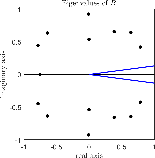
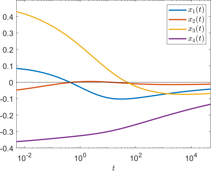
Figure 1: Left: Location of the eigenvalues of the matrix $B$ from Example 3.6 in the complex plane. The blue rays are oriented at an angle of $\pm\gamma\pi/2=\pm\pi/24$ from the positive real axis and hence indicate the boundary of the critical sector $\{z\in\mathbb{C}:|\arg z|\leq\gamma\pi/2\}$. Since all eigenvalues are outside of this sector, we can derive the asymptotic stability of the system. Right: Trajectories of the solution of the system (4) discussed in Example 3.6 where $\hat{\alpha}=(\frac{1}{2},\frac{1}{4},\frac{1}{3},\frac{1}{6})$ and the matrix $A$ is given in eq. (10) when the initial condition (5) is chosen as $x_{0}=(0.1,-0.1,0.5,-0.4)^{\mathrm{T}}$. Note that the horizontal axis is displayed in a logarithmic scale.

Remark 3.7.

The solution of Example 3.6 shown in the right part of Figure 1 has been computed numerically with Garrappa’s implementation of the implicit product integration rule of trapezoidal type [8]. It has been shown in [7, Section 5] that the stability properties of this method are sufficient to numerically reproduce the stability of the exact solution. The step size was chosen as $h=1/200$. We have also used this algorithm and the same step size for all other examples in the remainder of this paper.

4 The $\hat{\alpha}$-order spectrum: The case $\hat{\alpha}\in(0,1]^{n}$

Now we generalize our considerations to the case of systems of fractional differential equations with arbitrary (not necessarily rational) orders. To this end, we first devise a strategy for replacing the original (potentially irrational) orders by nearby rational numbers (see Subsection 4.1). The resulting problem can then be handled with the approach described in Section 3 above. Finally, in Subsection 4.2 we show how to transfer the results obtained in this way back to the originally given system.

4.1 Rational approximations of a fractional spectrum

Definition 4.1.

For a given matrix $A\in M_{n}(\mathbb{R})$, a multi-index $\hat{\alpha}=(\alpha_{1},\ldots,\alpha_{n})\in(0,1]^{n}$ and $\epsilon>0$, we call $\hat{\beta}=(\beta_{1},\ldots,\beta_{n})\in(0,1]^{n}\cap\mathbb{Q}^{n}$ an $\epsilon$-rational approximation of $\hat{\alpha}$ associated with $A$ if the following conditions are satisfied:

• $0<\beta_{i}\leq\alpha_{i}\leq 1$ for all $i\in N$.

• There exists a constant $R=R(A,\hat{\alpha},\epsilon)\geq 1$ such that $\sigma_{\hat{\alpha},\epsilon}^{2}(A)\cap\left\{z\in\mathbb{C}:|z|>R\right\}=\sigma_{\hat{\beta},\epsilon}^{2}(A)\cap\left\{z\in\mathbb{C}:|z|>R\right\}=\emptyset$.

• There is a constant $\rho=\rho(A,\hat{\alpha},\epsilon)\in(0,1)$ such that $\sigma_{\hat{\alpha}}(A)\cap\left\{z\in\mathbb{C}:|z|<\rho\right\}=\sigma_{\hat{\beta}}(A)\cap\left\{z\in\mathbb{C}:|z|<\rho\right\}=\emptyset$.

• For $R$ and $\rho$ chosen as above, we have

  $$\sup_{\rho\leq|z|\leq R}\,|z^{\alpha_{i}}-z^{\beta_{i}}|<\epsilon\text{ for all }i\in N.$$

Our first observation in this context establishes that this definition is actually meaningful.

Proposition 4.2.

Let $A\in M_{n}(\mathbb{R})$ such that $\det A\neq 0$ and let $\hat{\alpha}=(\alpha_{1},\ldots,\alpha_{n})\in(0,1]^{n}$. Then, for any $\epsilon>0$, there exists some $\hat{\beta}=(\beta_{1},\ldots,\beta_{n})\in(0,1]^{n}\cap\mathbb{Q}^{n}$ which is an $\epsilon$-rational approximation of $\hat{\alpha}$ associated with $A$.

Proof.

Put $l(\hat{\alpha})=\alpha_{1}+\ldots+\alpha_{n}$, $\nu(\hat{\alpha})=\min_{i\in N}\{\alpha_{i}\}$ and $\epsilon_{0}=\frac{1}{2}\nu(\hat{\alpha})$.

We define $\mathcal{F}(\hat{\alpha}):=\{\hat{\gamma}=(\hat{\gamma}_{1},\,\ldots,\hat{\gamma}_{n})\in(0,1]^{n}:0<\alpha_{i}-\epsilon_{0}\leq\hat{\gamma}_{i}\leq\alpha_{i}\text{ for all }i\in N\}$ and

$$R:=\max\left\{\left(\max_{i\in N}\{|a_{ii}|+r_{i}(A)+r_{i}(A^{\mathrm{T}})\}+\epsilon\right)^{1/{(\nu(\hat{\alpha})-\epsilon_{0})}},\max_{i\in N}\left(\frac{\epsilon}{\sqrt{2}}\right)^{1/\alpha_{i}},1\right\}$$ (11)

where, as in Theorem 2.3, we set $r_{i}(A)=\sum_{j\in N,j\neq i}|a_{ij}|$. Then, for any $\hat{\gamma}\in\mathcal{F}(\hat{\alpha})$ and $z\in\mathbb{C}$, $|z|>R$, we have for all $i\in N$

$$|z^{\hat{\gamma}_{i}}-a_{ii}| \geq|z|^{\hat{\gamma}_{i}}-|a_{ii}|>R^{\hat{\gamma}_{i}}-|a_{ii}|\geq R^{\alpha_{i}-\epsilon_{0}}-|a_{ii}|\geq R^{\nu(\hat{\alpha})-\epsilon_{0}}-|a_{ii}|$$

$$\geq|a_{ii}|+r_{i}(A)+r_{i}(A^{\mathrm{T}})+\epsilon-|a_{ii}|\geq\max\{r_{i}(A),r_{i}(A^{\mathrm{T}})\}+\epsilon.$$

Thus, by Theorem 2.5,

$$\sigma_{\hat{\gamma},\epsilon}^{2}(A)\cap\left\{z\in\mathbb{C}:|z|>R\right\}=\emptyset\quad\text{ for all }\hat{\gamma}\in\mathcal{F}(\hat{\alpha}).$$ (12)

Now take $\hat{\mathcal{B}_{n}}:=\{0,1\}^{n}$ and $\mathcal{B}_{n}:=\left\{\xi\in\hat{\mathcal{B}_{n}}:\xi\neq(0,\ldots,0)\text{and }\xi\neq(1,\ldots,1)\right\}$. For any $\hat{\gamma}\in\mathcal{F}(\hat{\alpha})$, we have

$$\det(z^{\hat{\gamma}}I-A)=z^{l(\hat{\gamma})}+\sum_{\xi\in\mathcal{B}_{n}}c_{\xi}z^{\left<\hat{\gamma},\xi\right>}+(-1)^{n}\det A,$$ (13)

where $\left\langle\cdot\,,\cdot\right\rangle$ is the usual scalar product on $\mathbb{R}^{n}$. If $\xi\in\mathcal{B}_{n}$, $\xi_{i_{1}}=\ldots=\xi_{i_{r}}=1$ for some $\{i_{1},\ldots,i_{r}\}\subset N$ and $\xi_{i}=0$ for all $i\in N\setminus\{i_{1},\ldots,i_{r}\}$, then $z^{\left<\hat{\gamma},\xi\right>}=z^{\hat{\gamma}_{i_{1}}}\cdots z^{\hat{\gamma}_{i_{r}}}$. By using the same arguments as in calculating the coefficient of the term $s^{p_{i_{1}}}\cdots s^{p_{i_{r}}}$ in the expansion of $\det(s^{\hat{p}}I-A)$ above, we obtain $c_{\xi}=(-1)^{r}\det A_{(i_{1},\ldots,i_{r})}$, where $A_{(i_{1},\ldots,i_{r})}$ is obtained from $A$ by removing the rows $i_{1},\ldots,i_{r}$ and the columns $i_{1},\ldots,i_{r}$.

Let $c=\max\{1,\max_{\xi\in\mathcal{B}_{n}}|c_{\xi}|\}$ and $\rho_{1}=\min\left\{\left(\frac{|\det A|}{(2^{n}-1)c}\right)^{1/{(\nu(\hat{\alpha})-\epsilon_{0})}},\frac{1}{2}\right\}$. Because $\det A\neq 0$, we may conclude that $0<\rho_{1}<1$. Moreover, for all $\hat{\gamma}\in\mathcal{F}(\hat{\alpha})$ and $|z|<\rho_{1}<1$,

$$\max\left\{|z|^{\hat{\gamma}_{1}+\ldots+\hat{\gamma}_{n}},\max_{\xi\in\mathcal{B}_{n}}|z|^{\left<\hat{\gamma},\xi\right>}\right\} \leq|z|^{\min_{i\in N}\{\hat{\gamma}_{i}\}}\leq|z|^{\nu(\hat{\alpha})-\epsilon_{0}}$$

$$<\rho_{1}^{\nu(\hat{\alpha})-\epsilon_{0}}\leq\frac{|\det A|}{(2^{n}-1)c}.$$

Hence, by (13), the following estimates hold

$$|\det(z^{\hat{\gamma}}I-A)| =\left|z^{\gamma_{1}+\ldots\gamma_{n}}+\sum_{\xi\in\mathcal{B}_{n}}c_{\xi}z^{\left<\hat{\gamma},\xi\right>}+(-1)^{n}\det A\right|$$

$$\geq|(-1)^{n}\det A|-|z^{\gamma_{1}+\ldots+\gamma_{n}}|-\left|\sum_{\xi\in\mathcal{B}_{n}}c_{\xi}z^{\left<\hat{\gamma},\xi\right>}\right|$$

$$\geq|\det A|-|z|^{\hat{\gamma}_{1}+\ldots+\hat{\gamma}_{n}}-\sum_{\xi\in\mathcal{B}_{n}}|c_{\xi}|\cdot|z|^{\left<\hat{\gamma},\xi\right>}$$

$$>|\det A|-(2^{n}-1)c\frac{|\det A|}{(2^{n}-1)c}=0$$

for any $\hat{\gamma}\in\mathcal{F}(\alpha)$ and $|z|<\rho_{1}<1$. From this, we see

$$\sigma_{\hat{\gamma}}(A)\cap\{z\in\mathbb{C}:|z|<\rho_{1}\}=\emptyset\text{ for all }\hat{\gamma}\in\mathcal{F}(\hat{\alpha}).$$ (14)

Put $\rho_{2}=\min\left\{\left(\frac{\epsilon}{2}\right)^{1/(\nu(\hat{\alpha})-\epsilon_{0})},\frac{1}{2}\right\}$. Then $0<\rho_{2}<1$. Furthermore, for all $\hat{\gamma}\in\mathcal{F}(\hat{\alpha})$ and $|z|<\rho_{2}<1$, we have

$$|z^{\alpha_{i}}-z^{\hat{\gamma}_{i}}| \leq|z|^{\alpha_{i}}+|z|^{\hat{\gamma}_{i}}\leq\rho_{2}^{\alpha_{i}}+\rho_{2}^{\hat{\gamma}_{i}}\leq 2\rho_{2}^{\nu(\hat{\alpha})-\epsilon_{0}}<\epsilon\text{ for all }i\in N.$$ (15)

Take $\rho=\min\{\rho_{1},\rho_{2}\}$, then $0<\rho<1$. Moreover, from (14) and (15), we conclude

$$\sup_{|z|<\rho}|z^{\alpha_{i}}-z^{\hat{\gamma}_{i}}| <\epsilon\text{ for all }i\in N\text{ and }$$ (16)

$$\sigma_{\hat{\gamma}}(A)\cap\{z\in\mathbb{C}:|z|<\rho\} =\emptyset\text{ for all }\hat{\gamma}\in\mathcal{F}(\hat{\alpha}).$$ (17)

For all $z\in\mathbb{C}$, $\rho\leq|z|\leq R$, we use the polar coordinate form $z=r(\cos\varphi+{\mathrm{i}}\sin\varphi)$ with $\rho\leq r\leq R$ and $-\pi<\varphi\leq\pi$. Then, for any ${\tilde{\alpha}}=(\tilde{\alpha}_{1},\dots,\tilde{\alpha}_{n})^{\rm T}\in(0,1]^{n}$, we see

$$\left|z^{\alpha_{i}}-z^{\tilde{\alpha}_{i}}\right|^{2} =\left|\left(r^{\alpha_{i}}\cos(\alpha_{i}\varphi)-r^{{\tilde{\alpha_{i}}}}\cos(\tilde{\alpha}_{i}\varphi)\right)+{\mathrm{i}}\left(r^{\alpha_{i}}\sin(\alpha_{i}\varphi)-r^{\tilde{\alpha}_{i}}\sin(\tilde{\alpha}_{i}\varphi)\right)\right|^{2}$$

$$=\left(r^{\alpha_{i}}\cos(\alpha_{i}\varphi)-r^{\tilde{\alpha}_{i}}\cos(\tilde{\alpha}_{i}\varphi)\right)^{2}+\left(r^{\alpha_{i}}\sin(\alpha_{i}\varphi)-r^{\tilde{\alpha}_{i}}\sin(\tilde{\alpha}_{i}\varphi)\right)^{2}$$

$$=r^{2\alpha_{i}}+r^{2\tilde{\alpha}_{i}}-2r^{\alpha_{i}+\tilde{\alpha}_{i}}\left(\cos(\alpha_{i}\varphi)\cos(\tilde{\alpha}_{i}\varphi)+\sin(\alpha_{i}\varphi)\sin(\tilde{\alpha}_{i}\varphi)\right)$$

$$=r^{2\alpha_{i}}+r^{2\tilde{\alpha}_{i}}-2r^{\alpha_{i}+\tilde{\alpha}_{i}}\cos\left((\alpha_{i}-\tilde{\alpha}_{i})\varphi\right)$$

$$=\left(r^{\alpha_{i}}-r^{\tilde{\alpha}_{i}}\right)^{2}+2r^{\alpha_{i}+\tilde{\alpha}_{i}}\left(1-\cos\left((\alpha_{i}-\tilde{\alpha}_{i})\varphi\right)\right).$$ (18)

For each $i\in N$, we set $\delta_{1,i}=\log_{R}\left(1+\epsilon/(\sqrt{2}R^{\alpha_{i}})\right)>0$. Then, for all $\hat{\hat{\alpha}}\in(0,1]^{n}$ such that $0\leq\alpha_{i}-\hat{\hat{\alpha_{i}}}<\delta_{1,i}$ for all $i\in N$ and any $\rho\leq r\leq R$, we have

$$r^{\alpha_{i}-\hat{\hat{\alpha_{i}}}}-1 \leq R^{\alpha_{i}-\hat{\hat{\alpha_{i}}}}-1<R^{\log_{R}\left(1+\frac{\epsilon}{\sqrt{2}R^{\alpha_{i}}}\right)}-1=\frac{\epsilon}{\sqrt{2}R^{\alpha_{i}}}$$ (19)

for all $i\in N$. Because of (11), we know that $\epsilon/(\sqrt{2}R^{\alpha_{i}})<1$ for all $i\in N$. For each $i\in N$, let $\delta_{2,i}=\log_{\rho}\left(1-\frac{\epsilon}{\sqrt{2}R^{\alpha_{i}}}\right)>0$. Then, for any $\tilde{\tilde{\alpha}}\in(0,1]^{n}$ satisfying $0\leq\alpha_{i}-\tilde{\tilde{\alpha_{i}}}<\delta_{2,i}$ for all $i\in N$ and all $\rho\leq r\leq R$, we have

$$r^{\alpha_{i}-\tilde{\tilde{\alpha_{i}}}}-1\geq\rho^{\alpha_{i}-\tilde{\tilde{\alpha_{i}}}}-1>\rho^{\log_{\rho}\left(1-\epsilon/(\sqrt{2}R^{\alpha_{i}})\right)}-1=-\frac{\epsilon}{\sqrt{2}R^{\alpha_{i}}}.$$ (20)

Let $\delta_{1}=\min\left\{\delta_{1,i},\delta_{2,i}:i\in N\right\}>0$. By combining (19) and (20), for any $\hat{\kappa}\in(0,1]^{n}$ such that $0\leq\alpha_{i}-\hat{\kappa}_{i}<\delta_{1}$ for all $i\in N$ and $\rho\leq r\leq R$, we find

$$-\frac{\epsilon}{\sqrt{2}R^{\alpha_{i}}}<r^{\alpha_{i}-\hat{\kappa}_{i}}-1<\frac{\epsilon}{\sqrt{2}R^{\alpha_{i}}}$$ (21)

for all $i\in N$. Thus, for any $\hat{\kappa}\in(0,1]^{n}$ with $0\leq\alpha_{i}-\hat{\kappa}_{i}<\delta_{1}$ for all $i\in N$ and $\rho\leq r\leq R$, we obtain

$$\left(r^{\alpha_{i}}-r^{\hat{\kappa}_{i}}\right)^{2}=r^{2\hat{\kappa}_{i}}\left(r^{\alpha_{i}-\hat{\kappa}_{i}}-1\right)^{2}\leq R^{2\alpha_{1}}\frac{\epsilon^{2}}{2R^{2\alpha_{i}}}=\frac{\epsilon^{2}}{2}$$ (22)

for all $i\in N$. By (11), we have $\epsilon/(2R^{\alpha_{i}})<1$ for all $i\in N$. Thus, $0<1-\epsilon^{2}/(4R^{2\alpha_{i}})<1$ for all $i\in N$, and for each $i\in N$, there exists some $\varphi_{i}\in(0,\pi/2)$ such that $\cos\varphi_{i}=1-\epsilon^{2}/(4R^{2\alpha_{i}})$. Define $\delta_{3,i}=\varphi_{i}/\pi>0$ for $i\in N$. For $\alpha^{*}\in(0,1]^{n}$ such that $0\leq\alpha_{i}-\alpha^{*}_{i}<\delta_{3,i}$ for all $i\in N$ and $-\pi<\varphi\leq\pi$, we have

$$-\varphi_{i}<-\pi(\alpha_{i}-\alpha^{*}_{i})\leq\varphi(\alpha_{i}-\alpha^{*}_{i})\leq\pi(\alpha_{i}-\alpha^{*}_{i})<\varphi_{i}$$

for all $i\in N$. Thus,

$$0\leq 1-\cos\left((\alpha_{i}-\alpha^{*}_{i})\varphi\right)<1-\cos\varphi_{i}=\frac{\epsilon^{2}}{4R^{2\alpha_{i}}}$$

for all $i\in N$. For any $\alpha^{*}\in(0,1]^{n}$ satisfying $0\leq\alpha_{i}-\alpha^{*}_{i}<\delta_{3,i}$ for all $i\in N$ and all $\rho\leq r\leq R$ and $-\pi<\varphi\leq\pi$, we find

$$2r^{\alpha_{i}+\alpha^{*}_{i}}\left(1-\cos\left((\alpha_{i}-\alpha^{*}_{i})\varphi\right)\right)<2R^{2\alpha_{i}}\frac{\epsilon^{2}}{4R^{2\alpha_{i}}}=\frac{\epsilon^{2}}{2},\;\forall i\in N.$$ (23)

Choosing $\delta_{2}=\min_{i\in N}\left\{\delta_{3,i}\right\}$ and $\delta=\min\left\{\delta_{1},\delta_{2},\epsilon_{0}\right\}$, we see that $\delta>0$. On the other hand, using (4.1), (22) and (23), for any $\hat{\gamma}\in\mathcal{F}(\hat{\alpha})$ such that $0\leq\alpha_{i}-\hat{\gamma}_{i}<\delta$ for all $i\in N$ and all $z\in\mathbb{C}$ with $\rho\leq|z|\leq R$, we have

$$\left|z^{\alpha_{i}}-z^{\hat{\gamma}_{i}}\right|<\epsilon$$ (24)

for all $i\in N$. Thus, for $\hat{\gamma}\in(0,1]^{n}$ with $0\leq\alpha_{i}-\hat{\gamma}_{i}<\delta$ for all $i\in N$, we get

$$\sup_{\rho\leq|z|\leq R}\,\,\left|z^{\alpha_{i}}-z^{\hat{\gamma}_{i}}\right|<\epsilon$$ (25)

for all $i\in N$.

Due to the density of $\mathbb{Q}$ in $\mathbb{R}$, there exists $\hat{\beta}\in(0,1]^{n}\cap\mathbb{Q}^{n}$ such that $0\leq\alpha_{i}-\beta_{i}<\delta$ for all $i\in N$. We will prove that $\hat{\beta}$ is a rational approximation of $\hat{\alpha}$. Indeed, since $0<\beta_{i}\leq\alpha_{i}\leq 1$, the condition (i) in Definition 4.1 is satisfied. Since $\delta\leq\epsilon_{0}$, we have that $0<\alpha_{i}-\epsilon_{0}\leq\beta_{i}\leq\alpha_{i}$ for all $i\in N$. This implies $\hat{\beta}\in\mathcal{F}(\hat{\alpha})$. Obviously $\hat{\alpha}\in\mathcal{F}(\hat{\alpha})$. So, according to (12),

$$\sigma_{\hat{\alpha},\epsilon}^{2}(A)\cap\left\{z\in\mathbb{C}:|z|>R\right\}=\emptyset\text{ and }\sigma_{\hat{\beta},\epsilon}^{2}(A)\cap\left\{z\in\mathbb{C}:|z|>R\right\}=\emptyset.$$ (26)

Therefore, the condition (ii) in Definition 4.1 is satisfied. Next, since $\hat{\beta},\hat{\alpha}\in\mathcal{F}(\hat{\alpha})$, by (16), we have

$$\sup_{|z|<\rho}|z^{\alpha_{i}}-z^{\beta_{i}}|<\epsilon$$ (27)

for all $i\in N$, and (17) implies

$$\sigma_{\hat{\alpha}}(A)\cap\{z\in\mathbb{C}:|z|<\rho\}=\emptyset\text{ and }\sigma_{\hat{\beta}}(A)\cap\{z\in\mathbb{C}:|z|<\rho\}=\emptyset.$$ (28)

Therefore, the condition (iii) in Definition 4.1 is satisfied. Finally, since $0\leq\alpha_{i}-\beta_{i}<\delta$ for all $i\in N$, by (25) we have

$$\sup_{\rho\leq|z|\leq R}\,\,\left|z^{\alpha_{i}}-z^{\beta_{i}}\right|<\epsilon$$ (29)

for all $i\in N$. Hence, the condition (iv) in Definition 4.1 is satisfied. ∎

The above proposition actually shows us a way to find rational approximations of $\hat{\alpha}$ associated with a matrix $A$. Indeed, based on these considerations, we can propose the following algorithm to find an $\epsilon$-rational approximation of $\hat{\alpha}$ associated with a matrix $A$.

Algorithm 1

 Input: Matrix $A$, multi-index $\hat{\alpha}=(\alpha_{1},\ldots,\alpha_{n})$ and a constant $\epsilon>0$.

Step 1: Put $a=\frac{1}{2}\min_{i=1,\ldots,n}\{\alpha_{i}\}$ and $b=\max_{i=1,\ldots,n}\{\alpha_{i}\}$.

Step 2: Calculate all the principal minors and the determinant of $A$. Then compare the calculated numbers with each other and with $1$ to find the largest number which is then assigned to $c$.

Step 3: Calculate the following parameters:

$$R =\max\left\{\left(\max_{i\in N}\{|a_{ii}|+r_{i}(A)+r_{i}(A^{\mathrm{T}})\}+\epsilon\right)^{1/a},\max_{i\in N}\left(\frac{\epsilon}{\sqrt{2}}\right)^{1/\alpha_{i}},1\right\},$$

$$\rho =\min\left\{\left(\frac{|\det A|}{(2^{n}-1)c}\right)^{1/a},\left(\frac{\epsilon}{2}\right)^{1/a},\frac{1}{2}\right\}.$$

Step 4: Calculate the following quantities:

$$\delta_{1}=\log_{R}\left(1+\frac{\epsilon}{\sqrt{2}R^{b}}\right),$$

$$\delta_{2}=\log_{\rho}\left(1-\frac{\epsilon}{\sqrt{2}R^{b}}\right),$$

$$\delta_{3}=\cos^{-1}\left(1-\frac{\epsilon^{2}}{4R^{2b}}\right).$$

and take $\delta=\min\{\delta_{1},\delta_{2},\delta_{3},a\}$.

Step 5: For each $i=1,\ldots,n$, find a rational number $\beta_{i}$ such that $\alpha_{i}-\delta<\beta_{i}\leq\alpha_{i}$.

Output: Multi-index $\hat{\beta}=(\beta_{1},\ldots,\beta_{n})$.

 

4.2 Equivalence between the fractional spectrum and its rational approximation

Consider a matrix $A\in M_{n}(\mathbb{R})$ and a multi-index $\hat{\alpha}\in(0,1]^{n}$. Inspired by the definition of the spectral radius of a matrix and the applications of this concept in the theory of ordinary differential equations, see e.g., [9, 16], we propose the definition

$$\delta_{\hat{\alpha}}^{2}(A) :=\inf\left\{\|E\|_{2}:E\in M_{n}(\mathbb{C}),\sigma_{\hat{\alpha}}(A+E)\cap\mathbb{C}_{\geq 0}\neq\emptyset\right\}.$$

Suppose further that $\sigma_{\hat{\alpha}}(A)\subset\mathbb{C}_{-}$. Then, similar to [9, Proposition 3.1], we have

$$\delta_{\hat{\alpha}}^{2}(A) =\inf\left\{\|E\|_{2}:E\in M_{n}(\mathbb{C})\text{ and }\sigma_{\hat{\alpha}}(A+E)\cap{\mathrm{i}}\mathbb{R}\neq\emptyset\right\}$$

$$=\inf\left\{\epsilon:\sigma_{\hat{\alpha},\epsilon}^{2}(A)\cap{\mathrm{i}}\mathbb{R}\neq\emptyset\right\}$$

$$=\inf\left\{\epsilon:\text{there exists some }z\in{\mathrm{i}}\mathbb{R}\text{ such that }\|(z^{\hat{\alpha}}I-A)^{-1}\|_{2}^{-1}=\epsilon\right\}$$

$$=\min_{\Re(z)=0}\,\|(z^{\hat{\alpha}}I-A)^{-1}\|_{2}^{-1}.$$ (30)

Remark 4.3.

From the definition of $\delta_{\hat{\alpha}}^{2}(A)$, we see that $\sigma_{\hat{\alpha}}(A+E)\subset\mathbb{C}_{-}$ if $\|E\|_{2}<\delta_{\hat{\alpha}}^{2}(A)$ for all $E\in M_{n}(\mathbb{C})$.

Remark 4.4.

If $A\in M_{n}(\mathbb{R})$ and $\sigma_{\hat{\alpha}}(A)\subset\mathbb{C}_{-}$, then $\det(z^{\hat{\alpha}}I-A)\neq 0$ whenever $\Re(z)=0$. Thus $\|(z^{\hat{\alpha}}I-A)^{-1}\|_{2}^{-1}>0$ for all $z\in\mathbb{C}$ with $\Re(z)=0$ and $\min_{\Re(z)=0}\|(z^{\hat{\alpha}}I-A)^{-1}\|_{2}^{-1}>0$, which together with (4.2) implies that $\delta_{\hat{\alpha}}^{2}{(A)}>0$.

Remark 4.5.

Assume that $A\in M_{n}(\mathbb{R})$ and $\sigma_{\hat{\alpha}}(A)\subset\mathbb{C}_{-}$. Let $\epsilon>0$ such that $\sigma_{\hat{\alpha},\epsilon}^{2}(A)\subset\mathbb{C}_{-}$. Then, due to (2), we obtain that $\sigma_{\hat{\alpha}}(A+E)\subset\sigma_{\hat{\alpha},\epsilon}^{2}(A)\subset\mathbb{C}_{-}$ for every matrix $E\in M_{n}(\mathbb{C})$ provided that $\|E\|_{2}\leq\epsilon$. This implies $\delta_{\hat{\alpha}}^{2}(A)\geq\epsilon$. Thus, we have $\delta_{\hat{\alpha}}^{2}(A)\geq\sup\left\{\epsilon:\sigma_{\hat{\alpha},\epsilon}^{2}(A)\subset\mathbb{C}_{-}\right\}$.

Theorem 4.6.

For a given matrix $A\in M_{n}(\mathbb{R})$ and a multi-index $\hat{\alpha}\in(0,1]^{n}$, the following statements are equivalent:

• $\sigma_{\hat{\alpha}}(A)\subset\mathbb{C}_{-}$;

• There is a constant $h_{0}>0$ such that for all $\epsilon\in(0,h_{0})$ and all $\epsilon$-rational approximations $\hat{\beta}\in(0,1]^{n}\cap\mathbb{Q}^{n}$ of $\hat{\alpha}$ associated with $A$, we have $\sigma_{\hat{\beta}}(A)\subset\mathbb{C}_{-}$ and $\delta_{\hat{\beta}}^{2}(A)\geq\epsilon$;

• There exists an $\epsilon$-rational approximation $\hat{\beta}\in(0,1]^{n}\cap\mathbb{Q}^{n}$ of $\hat{\alpha}$ associated with $A$ such that $\sigma_{\hat{\beta}}(A)\subset\mathbb{C}_{-}$ and $\delta_{\hat{\beta}}^{2}(A)\geq\epsilon$.

Proof.

We will first prove that (i) $\Rightarrow$ (ii). Suppose $\sigma_{\hat{\alpha}}(A)\subset C_{-}$. Then, by Remark 4.4, we have $\delta_{\hat{\alpha}}^{2}(A)>0$. We thus choose $h_{0}=\delta_{\alpha}^{2}(A)/2>0$. According to Proposition 4.2, for all $0<\epsilon<h_{0}$ there exists some $\hat{\beta}\in(0,1]^{n}\cap\mathbb{Q}^{n}$ which is an $\epsilon$-rational approximation of $\hat{\alpha}$ associated with $A$. Therefore, $\hat{\beta}$ satisfies the conditions (i)–(iv) of Definition 4.1 whenever $\epsilon<h_{0}$. From (1), we have $\sigma_{\hat{\beta}}(A)\subset\sigma_{\hat{\beta},\epsilon}^{2}(A)$. Hence, by Definition 4.1 (ii), there exists a constant $R$ such that $\sigma_{\hat{\beta}}(A)\cap\{z\in\mathbb{C}:|z|>R\}=\emptyset$. Moreover, by Definition 4.1 (iii), there exists a constant $\rho$ such that $\sigma_{\hat{\beta}}(A)\cap\{z\in\mathbb{C}:|z|<\rho\}=\emptyset$. Consider any $z_{0}\in\sigma_{\hat{\beta}}(A)$. Then $\rho\leq|z|\leq R$ and

$$0=\det(z_{0}^{\beta}I-A)=\det(z_{0}^{\hat{\alpha}}I-A-(z_{0}^{\hat{\alpha}}I-z_{0}^{\hat{\beta}}I))=\det(z_{0}^{\hat{\alpha}}I-(A+E))$$ (31)

with $E=z_{0}^{\hat{\alpha}}I-z_{0}^{\hat{\beta}}I\in M_{n}(\mathbb{C})$. Thus, $z_{0}\in\sigma_{\hat{\alpha}}(A+E)$. Furthermore, according to Definition 4.1 (iv), we have $|z_{0}^{\alpha_{i}}-z_{0}^{\beta_{i}}|<\epsilon$ for all $i\in N$. Hence,

$$\|E\|_{2}=\|z_{0}^{\hat{\alpha}}I-z_{0}^{\hat{\beta}}I\|_{2}=\max_{i\in N}|z_{0}^{\alpha_{i}}-z_{0}^{\beta_{i}}|<\epsilon.$$ (32)

Since $\epsilon\leq h_{0}<\delta_{\hat{\alpha}}^{2}(A),$ by Remark 4.3 we see that $\sigma_{\hat{\alpha}}(A+E)\subset\mathbb{C}_{-}$ which implies $z_{0}\in\mathbb{C}_{-}$. Therefore, $\sigma_{\hat{\beta}}(A)\subset\mathbb{C}_{-}$. Next, we consider an arbitrary $z_{1}\in\sigma_{\hat{\beta},\epsilon}^{2}(A)$. According to (2), there exists $E_{1}\in M_{n}(\mathbb{C})$ with $\|E_{1}\|_{2}\leq\epsilon$ such that $z_{1}\in\sigma_{\hat{\beta}}(A+E_{1})$. This implies that

$$0 =\det(z_{1}^{\hat{\beta}}I-(A+E_{1}))=\det(z_{1}^{\hat{\alpha}}I-(A+E_{1})-(z_{1}^{\hat{\alpha}}I-z_{1}^{\hat{\beta}}I))$$

$$=\det(z_{1}^{\hat{\alpha}}I-(A+E_{1}+E_{2}))$$ (33)

where $E_{2}=z_{1}^{\hat{\alpha}}I-z_{1}^{\hat{\beta}}I\in M_{n}(\mathbb{C})$. Thus $z_{1}\in\sigma_{\hat{\alpha}}(A+E_{1}+E_{2})$.

On the other hand, since $z_{1}\in\sigma_{\hat{\beta},\epsilon}^{2}(A)$, Definition 4.1 (ii) implies $|z_{1}|\leq R$, and by Definition 4.1 (iv), we have $|z_{1}^{\alpha_{i}}-z_{1}^{\beta_{i}}|<\epsilon$ for all $i\in N$. Hence,

$$\|E_{2}\|_{2}=\|z_{1}^{\hat{\alpha}}I-z_{1}^{\hat{\beta}}I\|_{2}=\max_{i\in N}|z_{1}^{\alpha_{i}}-z_{1}^{\beta_{i}}|<\epsilon.$$ (34)

So, $\|E_{1}+E_{2}\|_{2}\leq\|E_{1}\|_{2}+\|E_{2}\|_{2}<\epsilon+\epsilon\leq 2h_{0}=\delta_{\hat{\alpha}}^{2}{A}$. Consequently, by Remark 4.3, we have $\sigma_{\hat{\alpha}}(A+E_{1}+E_{2})\subset\mathbb{C}_{-}$, and it follows that $z_{1}\in\mathbb{C}_{-}$. Hence, $\sigma_{\hat{\beta},\epsilon}^{2}(A)\subset\mathbb{C}_{-}$. By Remark 4.5, we have $\delta_{\hat{\beta}}^{2}(A)\geq\epsilon$. Thus, we have proved (i) $\Rightarrow$ (ii).

(ii) $\Rightarrow$ (iii) is obvious because of Proposition 4.2.

Finally, we will prove (iii) $\Rightarrow$ (i). Suppose that $\hat{\beta}$ is an $\epsilon$-rational approximation of $\hat{\alpha}$ associated with $A$ such that $\sigma_{\hat{\beta}}(A)\subset\mathbb{C}_{-}$ and $\delta_{\hat{\beta}}^{2}(A)\geq\epsilon$. Let $z_{2}\in\sigma_{\hat{\alpha}}(A)$ be arbitrary. Then,

$$0=\det(z_{2}^{\hat{\alpha}}I-A)=\det(z_{2}^{\hat{\beta}}I-A-(z_{2}^{\hat{\beta}}I-z_{2}^{\hat{\alpha}}I))=\det(z_{2}^{\hat{\beta}}I-(A+E_{3}))$$ (35)

where $E_{3}=z_{2}^{\hat{\beta}}I-z_{2}^{\hat{\alpha}}I\in M_{n}(\mathbb{C})$. Thus, $z_{2}\in\sigma_{\hat{\beta}}(A+E_{3})$. On the other hand, by (1), we have $\sigma_{\hat{\alpha}}(A)\subset\sigma_{\hat{\alpha},\epsilon}^{2}(A)$. Since $\beta$ is an $\epsilon$-rational approximation of $\hat{\alpha}$ associated with $A$, according to Definition 4.1 (ii) and (iii), there exist constants $\rho$ and $R$ with $0<\rho<1<R$ such that $\rho\leq|z_{2}|\leq R$. Then, by Definition 4.1 (iv), we have $|z_{2}^{\alpha_{i}}-z_{2}^{\beta_{i}}|<\epsilon$ for all $i\in N$ which implies that

$$\|E_{3}\|_{2}=\|(z_{2}^{\hat{\beta}}-z_{2}^{\hat{\alpha}})I\|_{2}=\max_{i\in N}|z_{2}^{\alpha_{i}}-z_{2}^{\beta_{i}}|<\epsilon.$$ (36)

Since $\epsilon<\delta_{\hat{\beta}}^{2}(A)$, by Remark 4.3 we see that $\sigma_{\hat{\beta}}(A+E_{3})\subset\mathbb{C}_{-}$. Hence, $z_{2}\in\mathbb{C}_{-}$ and therefore, since $z_{2}$ was an arbitrary element of $\sigma_{\hat{\alpha}}(A)$, we can conclude that $\sigma_{\hat{\alpha}}(A)\subset\mathbb{C}_{-}$. Thus, we have completed the proof that (iii) $\Rightarrow$ (i) and hence also the proof of the complete theorem. ∎

As discussed above, we have given a criterion for testing whether the fractional spectrum of a matrix is lying in the open left half of the complex plane. This criterion is based on rational approximations of the fractional spectrum. An important step in this process is to estimate the positive lower bounds of $\delta_{\hat{\alpha}}^{2}(A)$ to find a suitable approximation. Now we will discuss in detail a case where the lower bound estimate for $\delta_{\hat{\alpha}}^{2}(A)$ is explicitly specified and thereby establish an algorithm that checks whether $\sigma_{\hat{\alpha}}(A)$ is in $\mathbb{C}_{-}$.

Proposition 4.7.

Let $A\in M_{n}(\mathbb{R})$ and $\hat{\alpha}\in(0,1]^{n}$. In addition, suppose that $\sigma_{\hat{\alpha}}(A)\subset\mathbb{C}_{-}$ and $\lambda_{\min}(-(A+A^{\mathrm{T}}))>0$, where $\lambda_{\min}(-(A+A^{\mathrm{T}}))$ is the smallest eigenvalue of the matrix $-(A+A^{\mathrm{T}})$. Then, $\delta_{\hat{\alpha}}^{2}(A)\geq\frac{1}{2}\lambda_{\min}(-(A+A^{\mathrm{T}}))>0$.

Proof.

In view of $\sigma_{\hat{\alpha}}(A)\subset\mathbb{C}_{-}$, by (4.2) and Remark 4.4 we have

$$\delta_{\hat{\alpha}}^{2}(A)=\min_{\Re(z)=0}\|\left(z^{\hat{\alpha}}I-A\right)^{-1}\|_{2}^{-1}>0.$$

This implies that

$$(\delta_{\hat{\alpha}}^{2}(A))^{-1}=\max_{\Re(z)=0}\|\left(z^{\hat{\alpha}}I-A\right)^{-1}\|_{2}>0.$$

From this relation we deduce that there exists some $\omega_{0}\in\mathbb{R}$ with the property that $\max_{\Re(z)=0}\|\left(z^{\hat{\alpha}}I-A\right)^{-1}\|_{2}=\|\left(({\mathrm{i}}\omega_{0})^{\hat{\alpha}}I-A\right)^{-1}\|_{2}$. Therefore, there exists $u_{0}\in\mathbb{C}^{n}$ with $\|u_{0}\|_{2}=1$ such that $\|\left(({\mathrm{i}}\omega_{0})^{\hat{\alpha}}I-A\right)^{-1}\|_{2}=\|\left(({\mathrm{i}}\omega_{0})^{\hat{\alpha}}I-A\right)^{-1}u_{0}\|$. Using the notation $x=\left(({\mathrm{i}}\omega_{0})^{\hat{\alpha}}I-A\right)^{-1}u_{0}$, we see that $\|x\|=(\delta_{\hat{\alpha}}^{2}(A))^{-1}>0$, so $x\neq 0$. Applying the min-max theorem to the Hermitian matrix $-(A+A^{\mathrm{T}})=-(A+A^{*})$ (note that $A$ is a real matrix by assumption), we have

$$\lambda_{\min}(-(A+A^{*}))\|x\|_{2}^{2} \leq\left<(-(A+A^{*})x,x\right>$$

$$\leq\left<\left(({\mathrm{i}}\omega_{0})^{\hat{\alpha}}I-A+(({\mathrm{i}}\omega_{0})^{\hat{\alpha}}I-A)^{*}-2\Re\left(({\mathrm{i}}\omega_{0})^{\hat{\alpha}}I\right)\right)x,x\right>$$

where $\Re\left(({\mathrm{i}}\omega_{0})^{\hat{\alpha}}I\right)=\mathop{\mathrm{diag}}(|\omega_{0}^{\alpha_{1}}|\cos\frac{\alpha_{1}\pi}{2},\ldots,|\omega_{0}^{\alpha_{n}}|\cos\frac{\alpha_{n}\pi}{2})$. Thus,

$$\lambda_{\min}(-(A+A^{*}))\|x\|_{2}^{2}+2\left<\Re\left(({\mathrm{i}}\omega_{0})^{\alpha}I\right)x,x\right> \leq\left<\left((i\omega_{0})^{\hat{\alpha}}I-A+(({\mathrm{i}}\omega_{0})^{\hat{\alpha}}I-A)^{*}\right)x,x\right>$$

$$=2\Re\left(\left<\left(({\mathrm{i}}\omega_{0})^{\hat{\alpha}}I-A\right)x,x\right>\right)$$

$$=2\Re\left<u_{0},x\right>\leq 2|\Re\left<u_{0},x\right>|\leq 2|\left<u_{0},x\right>|$$

$$\leq 2\|u_{0}\|_{2}\|x\|_{2}=2\|x\|_{2}.$$ (37)

On the other hand,

$$2\left<\Re\left(({\mathrm{i}}\omega_{0})^{\hat{\alpha}}I\right)x,x\right> =\left<\left(|\omega_{0}|^{\alpha_{1}}\cos\frac{\alpha_{1}\pi}{2}x_{1},\ldots,|\omega_{0}|^{\alpha_{n}}\cos\frac{\alpha_{n}\pi}{2}x_{n}\right)^{\mathrm{T}},x\right>$$

$$=\sum_{i=1}^{n}|\omega_{0}|^{\alpha_{i}}\cos\frac{\alpha_{i}\pi}{2}|x_{i}|^{2}\geq 0.$$ (38)

Using (4.2) and (4.2), we see

$$\lambda_{\min}(-(A+A^{*}))||x||_{2}^{2}\leq 2\|x\|_{2},$$

which implies that $\|x\|_{2}^{-1}\geq\frac{1}{2}\lambda_{\min}(-(A+A^{*}))$. Recalling once again that $A\in M_{n}(\mathbb{R})$, we conclude $\delta_{\hat{\alpha}}^{2}(A)\geq\frac{1}{2}\lambda_{\min}(-(A+A^{\mathrm{T}}))$. The proof is complete. ∎

The arguments of our proofs allow us to formulate an algorithm to check, for matrices $A$ satisfying the condition $\lambda_{\min}(-(A+A^{\mathrm{T}}))>0$, whether $\sigma_{\hat{\alpha}}(A)$ lies in the open left half of the complex plane:

Algorithm 2

 Input: Matrix $A$ satisfying $\lambda_{\min}(-(A+A^{\mathrm{T}}))>0$, and a multi-index $\hat{\alpha}$.

Step 1: Calculate $\lambda_{\min}(-(A+A^{\mathrm{T}}))$ and put $h_{0}=\frac{1}{2}\lambda_{\min}(-(A+A^{\mathrm{T}}))$.

Step 2: Apply Algorithm 1 using the matrix $A$, the multi-index $\hat{\alpha}$ and $\epsilon=h_{0}$ as input data to find $\hat{\beta}$ which is an $\epsilon$-rational approximation of $\hat{\alpha}$ associated with $A$.

Step 3: Check if $\sigma_{\hat{\beta}}(A)$ lies in the open left half of the complex plane. If $\sigma_{\hat{\beta}}(A)\subset\mathbb{C}_{-}$, we conclude that $\sigma_{\hat{\alpha}}(A)\subset\mathbb{C}_{-}$. If $\sigma_{\hat{\beta}}(A)\nsubseteq\mathbb{C}_{-}$, we conclude that $\sigma_{\hat{\alpha}}(A)\nsubseteq\mathbb{C}_{-}$.

Output: The result of Step 3, i.e. the information whether or not $\sigma_{\hat{\alpha}}(A)$ lies in the open left half of the complex plane.

 

Example 4.8.

To illustrate the proposed algorithms, we consider the system

$$^{C}D^{\hat{\alpha}}_{0^{+}}x(t)=Ax(t),\;t>0$$ (39)

with

$$A=\begin{pmatrix}-0.5&-0.2&-0.15&0.25\\ 0.15&-0.4&0.2&-0.15\\ 0.25&0.15&-0.6&0.3\\ 0.2&-0.1&-0.1&-0.3\\ \end{pmatrix}$$

(as in Example 3.6) and the multi-index $\hat{\alpha}=(\alpha_{1},\alpha_{2},\alpha_{3},\alpha_{4})=\left(\frac{128}{71\sqrt{13}},\frac{64}{71\sqrt{13}},\frac{90}{47\sqrt{33}},\frac{45}{47\sqrt{33}}\right)$. By direct calculations we have $\lambda_{\min}(-(A+A^{\mathrm{T}}))\approx 0.204$. We may therefore set $h_{0}=0.1$ and find the $0.1$-rational approximation $\hat{\beta}$ of $\hat{\alpha}$ associated with $A$ using Algorithm 1 as follows: We have $a=\frac{1}{2}\min_{i\in N}\{\alpha_{i}\}=\frac{45}{94\sqrt{33}}$, $b=\max_{i\in N}\{\alpha_{i}\}=\frac{128}{71\sqrt{13}}$ and $c=1$. By simple calculations, we get

$$R =(1.75+0.1)^{1/a}\approx 1606.922,$$

$$\rho =\left(\frac{3759}{80000\times 15}\right)^{1/a}\approx 8.94\times 10^{-31},$$

$$\delta_{1} =\log_{R}\left(1+\frac{\epsilon}{\sqrt{2}R^{b}}\right)\approx 0.000239,$$

$$\delta_{2} =\log_{\rho}\left(1-\frac{\epsilon}{\sqrt{2}R^{b}}\right)\approx 0.0000255,$$

$$\delta_{3} =\frac{1}{\pi}\cos^{-1}\left(1-\frac{\epsilon^{2}}{4R^{2b}}\right)\approx 0.000561.$$

This implies that $\delta=\delta_{2}=0.0000255$. Furthermore, $0.4995\approx\alpha_{1}-\delta<\beta_{1}<\alpha_{1}\approx 0.50001$. Hence, we can take $\beta_{1}=1/2$. Similarly, we have $\beta_{2}=1/4$, $\beta_{3}=1/3$ and $\beta_{4}=1/6$ which shows that $\hat{\beta}=\left(\frac{1}{2},\frac{1}{4},\frac{1}{3},\frac{1}{6}\right)$ is a $0.1$-rational approximation of $\hat{\alpha}$ associated with $A$. From Example 3.6, we see that $\sigma_{\hat{\beta}}(A)\subset\mathbb{C}_{-}$ and thus $\sigma_{\hat{\alpha}}(A)\subset\mathbb{C}_{-}$. A plot of the corresponding solution function graphs is visually undistinguishable from the plot shown in Figure 1, therefore we do not show this explicitly here. But clearly, this indicates the asymptotic stability in the case discussed here too. This effect could have been expected because the difference between the system considered here and the system of Example 3.6 above is only a tiny change in the orders of the differential operators, and standard theoretical results [3, Theorem 6.22] show that—unless the generalized eigenvalues of the original system had been so close to the boundary of the stability region that this change had made them move to the other side of the boundary, which is not the case here—such small changes only lead to correspondingly small changes in the solutions.

5 Asymptotic behavior of solutions to non-commensurate fractional-order nonlinear systems

Based on the developments above, we can now state some results about the stability of fractional multi-order differential systems. We will begin with a discussion of the case of a linear system and deal with the nonlinear case afterwards.

5.1 Inhomogeneous linear systems

Consider the inhomogeneous linear mixed-order system

$$^{C}D^{\hat{\alpha}}_{0^{+}}x(t)=Ax(t)+f(t),\;t>0$$ (40)

with the initial condition

$$x(0)=x^{0}\in\mathbb{R}^{n},$$ (41)

where $\hat{\alpha}=(\alpha_{1},\alpha_{2},\ldots\alpha_{n})\in(0,1]^{n}$, $A\in\mathbb{R}^{n\times n}$ and $f:[0,\infty)\rightarrow\mathbb{R}^{n}$ is continuous and exponentially bounded, that is, there exist constants $M,\gamma>0$ such that $\|f(t)\|\leq Me^{\gamma t}$ for all $t\in[0,\infty)$. We will first establish a variation of constants formula for the problem (40)-(41). To this end, we may generalize the approach described in [6, Subsection 2.2] for the case $n=2$, i.e. we take the Laplace transform on both sides of the system (40) and incorporate the initial condition (41) to get the algebraic equation

$$(s^{\hat{\alpha}}I)X(s)-(s^{\hat{\alpha}-1}I)x^{0}=AX(s)+F(s),$$ (42)

where $s^{\hat{\alpha}}I=\mathop{\mathrm{diag}}(s^{\alpha_{1}},\ldots,s^{\alpha_{n}})$, $s^{\hat{\alpha}-1}I=\mathop{\mathrm{diag}}(s^{\alpha_{1}-1},\ldots,s^{\alpha_{n}-1})$ and $X(\cdot)$ and $F(\cdot)$ are the Laplace transforms of $x(\cdot)$ and $f(\cdot)$, respectively. Thus,

$$X(s)=(s^{\hat{\alpha}}I-A)^{-1}\left((s^{\alpha_{1}-1}x^{0}_{1},\ldots,s^{\alpha_{n}-1}x^{0}_{n})^{\mathrm{T}}+F(s)\right).$$ (43)

Since $(s^{\hat{\alpha}}I-A)^{-1}=\frac{1}{Q(s)}\left((-1)^{i+j}\Delta^{A}_{ij}(s)\right)_{n\times n}$, where $Q(s)=\det(s^{\hat{\alpha}}I-A)$ and $\Delta^{A}_{ij}(s)$ is the determinant of the matrix obtained from the matrix $s^{\hat{\alpha}}I-A$ by removing the $j$-th row and the $i$-th column, for each $i\in N$ we have

$$X_{i}(s)=\sum_{j=1}^{n}\frac{1}{Q(s)}\left((-1)^{i+j}\Delta^{A}_{ij}(s)\right)s^{\alpha_{j}-1}x^{0}_{j}+\sum_{j=1}^{n}\frac{1}{Q(s)}\left((-1)^{i+j}\Delta^{A}_{ij}(s)\right)F_{j}(s).$$ (44)

Next, we will explicitly calculate the terms $\Delta^{A}_{ij}(s)$. For $i=j$, we put

$$\widetilde{\hat{\alpha}^{i}}=(\alpha_{1},\ldots,\alpha_{i-1},\alpha_{i+1},\ldots,\alpha_{n})$$

and designate by $A_{(i;i)}$ the matrix obtained from the matrix $A$ by removing the $i$-th row and $i$-th column. Then,

$$\Delta^{A}_{ii}(s)=\det(s^{\widetilde{\hat{\alpha}^{i}}}I-A_{(i;i)}).$$

Proceeding much as in Section 3, we obtain

$$\Delta^{A}_{ii}(s)=\sum_{\eta\in\mathcal{B}^{n-1}}c^{(i;i)}_{\eta}s^{\left<\widetilde{\hat{\alpha}^{i}},\eta\right>}$$ (45)

where $\mathcal{B}^{n-1}=\{0,1\}^{n-1}$ and, for every $\eta\in\mathcal{B}^{n-1}$, the $c^{(i;i)}_{\eta}$ are constants that depend only on the matrix $A_{(i;i)}$. Put

$$\hat{\mathcal{B}}^{n}_{i}=\{\xi\in\mathcal{B}^{n}:\xi_{i}=0\}$$

where $\mathcal{B}^{n}=\{0,1\}^{n}$ as in the proof of Proposition 4.2. We see that

$$\left\{\left<\widetilde{\hat{\alpha}^{i}},\eta\right>:\eta\in\mathcal{B}^{n-1}\right\}=\left\{\left<\hat{\alpha},\xi\right>:\xi\in\hat{\mathcal{B}}^{n}_{i}\right\},$$

and thus

$$\Delta^{A}_{ii}=\sum_{\xi\in\hat{\mathcal{B}}^{n}_{i}}c^{(i;i)}_{\xi}s^{\left<\hat{\alpha},\xi\right>}.$$

Let

$$\widetilde{\mathcal{B}}^{n}_{i}=\left\{\nu\in\mathcal{B}^{n}:\nu_{i}=1\right\},$$

then

$$\Delta^{A}_{ii}s^{\alpha_{i}-1} =\sum_{\xi\in\hat{\mathcal{B}}^{n}_{i}}c^{(i;i)}_{\xi}s^{\left<\hat{\alpha},\xi\right>}s^{\alpha_{i}-1}=\sum_{\xi\in\hat{\mathcal{B}}^{n}_{i}}c^{(i;i)}_{\xi}s^{\left<\hat{\alpha},\xi\right>+\alpha_{i}-1}=\sum_{\nu\in\widetilde{\mathcal{B}}^{n}_{i}}c^{(i;i)}_{\nu}s^{\left<\hat{\alpha},\nu\right>-1}.$$ (46)

The last equality above is obtained because

$$\left\{\left<\hat{\alpha},\xi\right>+\alpha_{i}:\xi\in\hat{\mathcal{B}}^{n}_{i}\right\}=\left\{\left<\hat{\alpha},\nu\right>:\nu\in\widetilde{\mathcal{B}}^{n}_{i}\right\}.$$

Next, for $i,j\in N$ with $i\neq j$, we put

$$\widetilde{\alpha^{i}_{j}}=\begin{cases}(\alpha_{1},\ldots,\alpha_{i-1},\alpha_{i+1},\ldots,\alpha_{j-1},0,\alpha_{j+1},\ldots,\alpha_{n})&\text{ if }i<j,\\ (\alpha_{1},\ldots,\alpha_{j-1},0,\alpha_{j+1},\ldots,\alpha_{i-1},\alpha_{i+1},\ldots,\alpha_{n})&\text{ if }i>j,\end{cases}$$ (47)

and $\hat{A}=A+{\bf 1}_{ij}$ where ${\bf 1}_{ij}$ is the $n\times n$ matrix whose element at the $i$-th row and the $j$-th column is 1 while all other entries are 0. Then,

$$\Delta^{A}_{ij}=\det(s^{\widetilde{\alpha^{i}_{j}}}I-\hat{A}_{(j;i)}),$$

where $\hat{A}_{(j,i)}$ is the matrix obtained from the matrix $\hat{A}$ by omitting the $j$-th row and the $i$-th column. Thus,

$$\Delta^{A}_{ij}(s)=\sum_{\eta\in\mathcal{B}^{n-1}}c^{(i;j)}_{\eta}s^{\left<\widetilde{\hat{\alpha}^{i}_{j}},\eta\right>},$$ (48)

where, for every $\eta\in\mathcal{B}^{n-1}$, the $c^{(i;j)}_{\eta}$ are constants that depend only on the matrix $\hat{A}_{(j;i)}$. Put

$$\hat{\mathcal{B}}^{n}_{(i;j)}=\left\{\xi\in\mathcal{B}^{n}:\xi_{i}=\xi_{j}=0\right\}.$$

Then,

$$\left\{\left<\widetilde{\hat{\alpha}^{i}_{j}},\eta\right>:\eta\in\mathcal{B}^{n-1}\right\}=\left\{\left<\hat{\alpha},\xi\right>:\xi\in\hat{\mathcal{B}}^{n}_{(i;j)}\right\}.$$

Thus,

$$\Delta^{A}_{ij}(s)=\sum_{\xi\in\hat{\mathcal{B}}^{n}_{(i;j)}}c^{(i;j)}_{\xi}s^{\left<\hat{\alpha},\xi\right>}.$$ (49)

Similarly, writing

$$\widetilde{\mathcal{B}^{n}_{i;j}}=\left\{\zeta\in\mathcal{B}^{n}:\zeta_{i}=0,\zeta_{j}=1\right\},$$

we obtain

$$\Delta^{A}_{ij}s^{\alpha_{j}-1} =\sum_{\xi\in\hat{\mathcal{B}}^{n}_{(i;j)}}c^{(i;j)}_{\xi}s^{\left<\hat{\alpha},\xi\right>}s^{\alpha_{j}-1}=\sum_{\xi\in\hat{\mathcal{B}}^{n}_{(i;j)}}c^{(i;j)}_{\xi}s^{\left<\hat{\alpha},\xi\right>+\alpha_{j}-1}=\sum_{\zeta\in\widetilde{\mathcal{B}^{n}_{i;j}}}c^{(i;j)}_{\zeta}s^{\left<\hat{\alpha},\zeta\right>-1}.$$ (50)

The last equality in (50) is obtained by

$$\left\{\left<\hat{\alpha},\xi\right>+\alpha_{j}:\xi\in\hat{\mathcal{B}}^{n}_{(i;j)}\right\}=\left\{\left<\hat{\alpha},\zeta\right>:\zeta\in\widetilde{\mathcal{B}^{n}_{i;j}}\right\}.$$

Taking

$$\mathcal{M}_{i}=\left\{\lambda:\lambda=\left<\hat{\alpha},\nu\right>,\nu\in\widetilde{\mathcal{B}}^{n}_{i}\,\,\text{ or }\,\,\lambda=\left<\hat{\alpha},\zeta\right>,\zeta\in\widetilde{\mathcal{B}^{n}_{i;j}}\right\},$$

we have, for all $i\in N$,

$$\sum_{j=1}^{n}\frac{1}{Q(s)}\left((-1)^{i+j}\Delta^{A}_{ij}(s)\right)s^{\alpha_{j}-1}x^{0}_{j}=\sum_{\lambda\in\mathcal{M}_{i}}c^{i}_{\lambda}\frac{s^{\lambda}}{sQ(s)}$$ (51)

with certain uniquely determined constants $c^{i}_{\lambda}\in\mathbb{R}$. In much the same way, setting

$$\mathcal{N}_{i}=\left\{\beta:\beta=\left<\hat{\alpha},\xi\right>,\xi\in\hat{\mathcal{B}}^{n}_{i}\,\,\text{ or }\,\,\beta=\left<\hat{\alpha},\eta\right>,\eta\in\hat{\mathcal{B}}^{n}_{(i;j)}\right\},$$

we have

$$\sum_{j=1}^{n}\frac{1}{Q(s)}\left((-1)^{i+j}\Delta^{A}_{ij}(s)\right)F_{j}(s)=\sum_{\beta\in\mathcal{N}_{i}}c_{\beta}^{i}\frac{s^{\beta}}{Q(s)}F(s)$$ (52)

for every $i\in N$, where once again the real constants $c_{\beta}^{i}$ are uniquely determined. From (44), (51) and (52), we conclude

$$X_{i}(s)=\sum_{\lambda\in\mathcal{M}_{i}}c^{i}_{\lambda}\frac{s^{\lambda}}{sQ(s)}+\sum_{\beta\in\mathcal{N}_{i}}c_{\beta}^{i}\frac{s^{\beta}}{Q(s)}F(s).$$ (53)

Thus, defining

$$R_{i}^{\lambda}(t)=\mathcal{L}^{-1}\left\{\frac{s^{\lambda}}{sQ(s)}\right\}\text{ for }\lambda\in\mathcal{M}_{i},$$ (54)

and

$$S_{i}^{\beta}(t)=\mathcal{L}^{-1}\left\{\frac{s^{\beta}}{Q(s)}\right\}\text{ for }\beta\in\mathcal{N}_{i},$$ (55)

we get the variation of constants formula for the problem (40)-(41) as follows:

$$x_{i}(t)=\sum_{\lambda\in\mathcal{M}_{i}}c^{i}_{\lambda}R_{i}^{\lambda}(t)+\sum_{\beta\in\mathcal{N}_{i}}c_{\beta}^{i}(S_{i}^{\beta}*f_{i})(t),\quad i=1,2,\ldots,n.$$ (56)

To determine the asymptotic behaviour of the functions $x_{i}$ for $i\in N$—and hence the stability properties of the differential equation (40)—from eq. (56), we need to obtain information about the asymptotic behaviour of the functions $R^{\lambda}_{i}$ and $S^{\beta}_{i}$. For this purpose, we can argue in exactly the same way as in [6, Lemma 8]. This leads us to the following result.

Lemma 5.1.

Let $\hat{\alpha}\in(0,1]^{n}$. Put $\nu=\min\{\alpha_{1},\alpha_{2},\ldots,\alpha_{n}\}$. Assume that $\sigma_{\hat{\alpha}}(A)$ lies in the open left half of the complex plane. Then, for all $i\in N$, $\lambda\in\mathcal{M}_{i}$ and $\beta\in\mathcal{N}_{i}$, we have the following asymptotic behaviour:

$$R^{\lambda}_{i}(t) =O(t^{-\nu})\text{ as }t\to\infty,$$ (57)

$$S^{\beta}_{i}(t) =O(t^{-\nu-1})\text{ as }t\to\infty,$$ (58)

$$S^{\beta}_{i}(t) =O(t^{\nu-1})\text{ as }t\to 0.$$ (59)

Furthermore,

$$\int_{0}^{\infty}|S^{\beta}_{i}(t)|{\mathrm{d}}t<\infty.$$

Next, we apply the estimates of Lemma 5.1 to the derive an intermediate result that will in the next step allow us to describe the behaviour of the terms in the second sum on the right-hand side of formula (56), i.e. the asymptotic behaviour of the convolution of $S^{\beta}_{i}$ with continuous functions. This result is a direct generalization of [6, Theorem 3] and can be proved in the same manner.

Theorem 5.2.

Let $\hat{\alpha}\in(0,1]^{n}$, $\nu=\min\{\alpha_{1},\alpha_{2},\ldots,\alpha_{n}\}$ and $\beta\in\mathcal{N}_{i}$ for some $i\in N$. For a given continuous function $g:[0,\infty)\rightarrow\mathbb{R}$, we set

$$F^{\beta}_{i}(t):=(S^{\beta}_{i}*g)(t)=\int_{0}^{t}S^{\beta}_{i}(t-s)g(s){\mathrm{d}}s.$$

Suppose that $\sigma_{\hat{\alpha}}(A)\subset\mathbb{C}_{-}$. Then, the following statements are true.

• If $g$ is bounded then $F^{\beta}_{i}$ is also bounded.

• If $\lim_{t\to\infty}g(t)=0$ then $\lim_{t\to\infty}F^{\beta}_{i}(t)=0$.

• If there exists some $\eta>0$ such that $g(t)=O(t^{-\eta})$ as $t\to\infty$, then $F^{\beta}_{i}(t)=O(t^{-\mu})$ as $t\to\infty$ where $\mu=\min\{\nu,\eta\}$.

From the above assertions, we obtain the following results on the asymptotic behavior of solutions to the inhomogeneous linear mixed order system (40).

Theorem 5.3.

Consider the initial value problem (40)-(41) with $\hat{\alpha}\in(0,1]^{n}$. Set $\nu=\min\{\alpha_{1},\alpha_{2},\ldots,\alpha_{n}\}$ and assume that $\sigma_{\hat{\alpha}}(A)\subset\mathbb{C}_{-}$. Then the following assertions hold.

• If $f$ is bounded then the solution of the initial value problem is also bounded, no matter how the initial value vector $x^{0}$ in (41) is chosen.

• If $\lim_{t\to\infty}f(t)=0$ then the solutions of (40) converge to $0$ as $t\to\infty$ for any choice of the initial value vector $x^{0}$.

• If there is some $\eta>0$ such that $\|f(t)\|=O(t^{-\eta})$ as $t\to\infty$ then, for any initial value vector $x^{0}$, the solution $x(\cdot)$ of (40) satisfies $\|x(t)\|=O(t^{-\mu})$ as $t\to\infty$, where $\mu=\min\{\nu,\eta\}$.

Proof.

This is a straightforward generalization of [6, Theorem 4] that can be shown in an analog manner, using our Theorem 5.2. ∎

5.2 Nonlinear Systems

Finally, we consider the autonomous non-commensurate fractional-order nonlinear system

$$^{C}D^{\hat{\alpha}}_{0^{+}}x(t) =Ax(t)+f(x(t)),\quad t>0,$$ (60)

$$x(0) =x^{0}\in\Omega\subset\mathbb{R}^{n},$$ (61)

where $\hat{\alpha}=(\alpha_{1},\alpha_{2},\ldots,\alpha_{n})\in(0,1]^{n}$, $A=\left(a_{ij}\right)\in\mathbb{R}^{n\times n}$, $\Omega$ is an open subset of $\mathbb{R}^{n}$ with $0\in\Omega$, $f:\Omega\rightarrow\mathbb{R}^{n}$ is locally Lipschitz continuous at the origin such that $f(0)=0$ and $\lim_{r\to 0}l_{f}(r)=0$ with

$$l_{f}(r):=\sup_{x,y\in B(0,r),\;x\neq y}\frac{\|f(x)-f(y)\|}{\|x-y\|}.$$

Putting $g(t)=f(x(t))$ and repeating the arguments as in Subsection 5.1, we get the representation of the solution of the problem (60)

$$x_{i}(t)=\sum_{\lambda\in\mathcal{M}_{i}}c^{i}_{\lambda}R_{i}^{\lambda}(t)+\sum_{\beta\in\mathcal{N}_{i}}c_{\beta}^{i}(S_{i}^{\beta}*f_{i})(x(t)),\quad i=1,2,\ldots,n.$$ (62)

We recall here the Mittag-Leffler stability definition that was introduced in [6, Definition 2].

Definition 5.4.

The trivial solution of (60) is Mittag-Leffler stable if there exist positive constants $\gamma,m$ and $\delta$ such that for any initial condition $x^{0}\in B(0,\delta)$, the solution $\varphi(\cdot,x^{0})$ of the initial value problem (60)-(61) exists globally on the interval $[0,\infty)$ and

$$\max\left\{\sup_{t\in[0,1]}\|\varphi(t,x^{0})\|,\sup_{t\geq 1}t^{\gamma}\|\varphi(t,x^{0})\|\right\}\leq m.$$

By the same approach as in [6, Theorem 5], we obtain the Mittag-Leffler stability of the trivial solution of (60):

Theorem 5.5.

Consider the system (60). Assume that $\sigma_{\hat{\alpha}}(A)\subset\mathbb{C}_{-}$. Then the trivial solution of the system of equations (60) is Mittag-Leffler stable. More precisely, there exist constants $\delta,\epsilon>0$ such that the unique global solution $\varphi(\cdot,x^{0})$ of the initial value problem (60)–(61) satisfies the estimate $\sup_{t\geq 1}t^{\nu}\|\varphi(t,x^{0})\|\leq\epsilon$ with $\nu=\min\{\alpha_{1},\alpha_{2},\ldots,\alpha_{n}\}$ provided that $\|x^{0}\|<\delta$.

6 Examples

This section is devoted to introducing some examples to illustrate the validity of the two main results obtained in Section 5.

Example 6.1.

We consider the system

$${}^{C}D^{\hat{\alpha}}_{0^{+}}x(t) =Ax(t)+f(t),\;t>0,$$ (63)

$$x(0) =x^{0}\in\mathbb{R}^{4},$$ (64)

where

$$A=\begin{pmatrix}-0.5&-0.2&-0.15&0.25\\ 0.15&-0.4&0.2&-0.15\\ 0.25&0.15&-0.6&0.3\\ 0.2&-0.1&-0.1&-0.3\end{pmatrix},$$

$\hat{\alpha}=(\alpha_{1},\alpha_{2},\alpha_{3},\alpha_{4})=\left(\frac{128}{71\sqrt{13}},\frac{64}{71\sqrt{13}},\frac{90}{47\sqrt{33}},\frac{45}{47\sqrt{33}}\right)$ and $f(t)=(f_{1}(t),f_{2}(t),f_{3}(t),f_{4}(t))^{\mathrm{T}}$ with $f_{i}(t)=(1+t^{i})^{-1}$, $i=1,2,3,4$. As shown in Example 4.8, we see that $\sigma_{\hat{\alpha}}(A)\subset\mathbb{C}_{-}$. Moreover, $\|f(t)\|=O(t^{-1})$ as $t\to\infty$. Due to Theorem 5.3, the system (63) is globally attractive and the solution $\varphi(\cdot,x^{0})$ satisfies $\|\varphi(t,x^{0})\|=O(t^{-\frac{45}{47\sqrt{33}}})$ as $t\to\infty$ for any $x^{0}\in\mathbb{R}^{4}$. The left part of Figure 2 shows a plot of the solution for a specific initial condition.

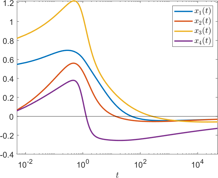
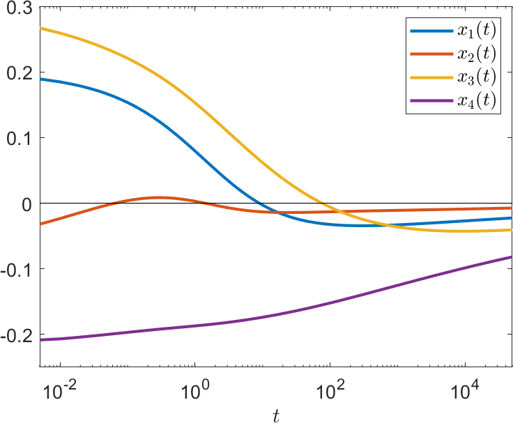
Figure 2: Left: Trajectories of the solution of (63) with the initial condition $x^{0}=(0.5,-0.3,0.7,-0.4)^{\mathrm{T}}$. Right: Trajectories of the solution of (65) with the initial condition $x^{0}=(0.2,-0.1,0.3,-0.25)^{\mathrm{T}}$. As in Figure 1, the horizontal axes in both plots are in a logarithmic scale.

Example 6.2.

Let us consider the system

$${}^{C}D^{\hat{\alpha}}_{0^{+}}x(t) =Ax(t)+f(x(t)),\;t>0,$$ (65)

$$x(0) =x^{0}\in\mathbb{R}^{4},$$ (66)

where $A$ and $\hat{\alpha}$ are as in Example 6.1 and $f(x(t))=(f_{1}(x(t)),f_{2}(x(t)),f_{3}(x(t)),f_{4}(x(t))^{\mathrm{T}}$ with $f_{1}(x)=x_{1}^{2}+x_{2}^{3}-x_{4}^{3}$, $f_{2}(x)=3x_{1}^{2}+4x_{2}^{3}-5x_{4}^{4}$, $f_{3}(x)=f_{4}(x)=x_{1}^{3}+3x_{2}^{3}$ for $x=(x_{1},\dots,x_{4})^{\rm T}\in\mathbb{R}^{4}$. Due to the fact that $\sigma_{\hat{\alpha}}(A)\subset\mathbb{C}_{-}$, Theorem 5.5 asserts that the system (65) is Mittag-Leffer stable. Furthermore, when the initial value vector $x^{0}$ is close enough to the origin, its solution $\varphi(\cdot,x^{0})$ converges to the origin at a rate no slower than $t^{-\frac{45}{47\sqrt{33}}}$ as $t\to\infty$. We provide plots of a solution in the right part of Figure 2.

To further illustrate the range of applicability of our results, we conclude with two more examples that have also been investigated with completely different methods elsewhere [4]. The fundamental difference between these following examples on the one hand and the examples discussed so far on the other hand is that we now look at coefficient matrices $A$ where some of the diagonal entries are zero (Example 6.3) or even positive (Example 6.4) while in the earlier examples all diagonal entries had been negative.

Example 6.3.

We consider the linear homogeneous system (4) with $\hat{\alpha}=(2/5,3/10,1/2)^{\mathrm{T}}$ and

$$A=\begin{pmatrix}-3&0&1.5\\ -0.5&0&0.5\\ 6&-1&-3\end{pmatrix}.$$

For this problem, we may apply Theorem 3.1 and find that $m=10$, i.e. $\gamma=1/10$, and $\hat{p}=(4,3,5)^{\mathrm{T}}$. Thus, the matrix $B$ is of size $(12\times 12)$. Taking into consideration that, in the notation of Section 3, $\det A_{(2)}=\det A_{(3)}=\det A_{(1,3)}=0$, the nonzero elements of its rightmost column are $(B)_{1,12}=-b_{0}=\det A=-3/4$, $(B)_{5,12}=-b_{4}=-\det A_{(1)}=-1/2$, $(B)_{8,12}=-b_{7}=\det A_{(1,2)}=-3$ and $(B)_{9,12}=-b_{8}=\det A_{(2,3)}=-3$. The eigenvalues $\lambda_{k}$ of $B$ are plotted in the left part of Figure 3 from which one can see that the property $|\arg\lambda_{k}|>\pi\gamma/2$ for all $k$, so that the system is asymptotically stable. A plot of one particular solution is shown in the right part of Figure 3. Here, the asymptotics can be seen to set in much earlier than in the previous examples.

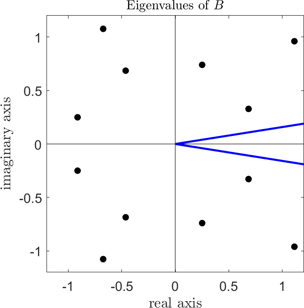
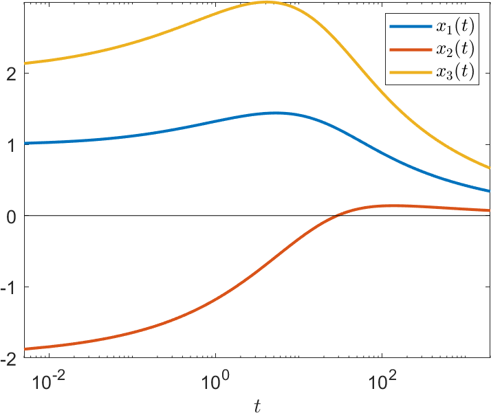
Figure 3: Left: Location of the eigenvalues of the matrix $B$ from Example 6.3 in the complex plane. The blue rays are oriented at an angle of $\pm\gamma\pi/2=\pm\pi/20$ from the positive real axis and hence indicate the boundary of the critical sector $\{z\in\mathbb{C}:|\arg z|\leq\gamma\pi/2\}$. Since all eigenvalues are outside of this sector, we can derive the asymptotic stability of the system. Right: Trajectories of the solution of Example 6.3 with the initial condition $x^{0}=(1,-2,2)^{\mathrm{T}}$.

Example 6.4.

In our last example, we consider the linear homogeneous system (4) with $\hat{\alpha}=(1/2,2/5,3/10)^{\mathrm{T}}$ and

$$A=\begin{pmatrix}-1&1&0\\ 0.25&-2&1\\ -2&0&1\end{pmatrix}.$$

For this problem, we may also apply Theorem 3.1 and find that $m=10$, i.e. $\gamma=1/10$, and $\hat{p}=(5,4,3)^{\mathrm{T}}$. Thus, the matrix $B$ is again of size $(12\times 12)$, and the nonzero elements of its rightmost column are, once more using the notation of Section 3, $(B)_{1,12}=-b_{0}=\det A=-1/4$, $(B)_{4,12}=-b_{3}=-\det A_{(3)}=-7/4$, $(B)_{5,12}=-b_{4}=-\det A_{(2)}=1$, $(B)_{6,12}=-b_{5}=-\det A_{(1)}=2$, $(B)_{8,12}=-b_{7}=\det A_{(2,3)}=-1$, $(B)_{9,12}=-b_{8}=\det A_{(1,3)}=-2$ and $(B)_{10,12}=-b_{9}=\det A_{(1,2)}=1$. The eigenvalues $\lambda_{k}$ of $B$ are plotted in the left part of Figure 4 from which one can see that the property $|\arg\lambda_{k}|>\pi\gamma/2$ for all $k$, so that the system is asymptotically stable. A plot of one particular solution is shown in the right part of Figure 4.

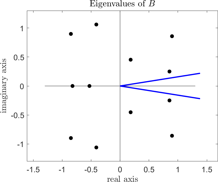
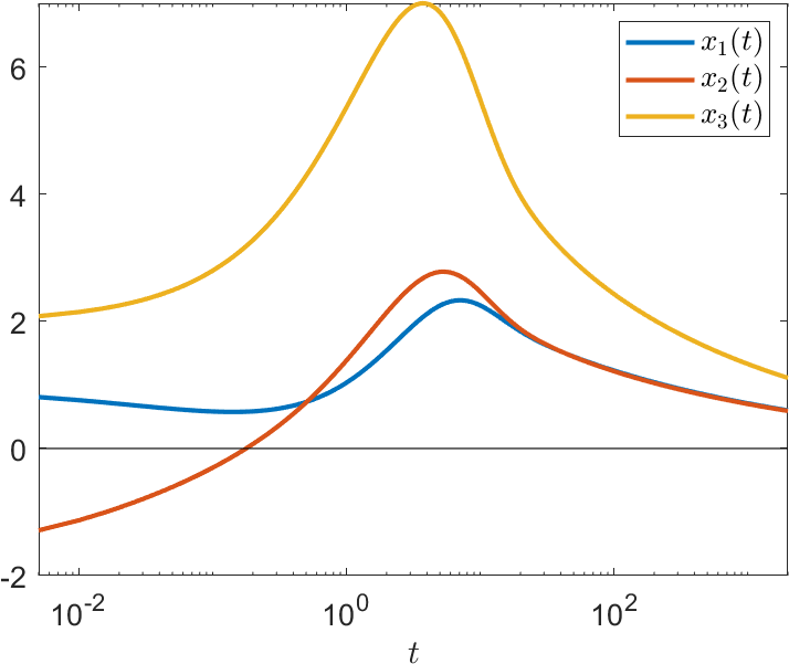
Figure 4: Left: Location of the eigenvalues of the matrix $B$ from Example 6.4 in the complex plane. The blue rays are oriented at an angle of $\pm\gamma\pi/2=\pm\pi/20$ from the positive real axis and hence indicate the boundary of the critical sector $\{z\in\mathbb{C}:|\arg z|\leq\gamma\pi/2\}$. Since all eigenvalues are outside of this sector, we can derive the asymptotic stability of the system. Right: Trajectories of the solution of Example 6.4 with the initial condition $x^{0}=(1,-2,2)^{\mathrm{T}}$.

References

- [1] N. D. Cong, Semigroup property of fractional differential operators and its applications. Discrete and Continuous Dynamical Systems - Series B, 28 (2023), pp. 1–19.
- [2] W. Deng, C. Li and J. Lü, Stability analysis of linear fractional differential system with multiple time delays. Nonlinear Dyn., 48 (2007), pp. 409–416.
- [3] K. Diethelm, The Analysis of Fractional Differential Equations. Berlin: Springer, 2010.
- [4] K. Diethelm and S. Hashemishahraki, Stability properties of multi-order fractional differential systems in 3D. Preprint, 2023.
- [5] K. Diethelm, S. Siegmund and H. T. Tuan, Asymptotic behavior of solutions of linear multi-order fractional differential equation systems. Fractional Calculus and Applied Analysis, 20 (2017), pp. 1165–1195.
- [6] K. Diethelm, H. D. Thai and H. T. Tuan, Asymptotic behaviour of solutions to non-commensurate fractional-order planar systems. Fractional Calculus and Applied Analysis, 25 (2022), pp. 1324–1360.
- [7] R. Garrappa, Trapezoidal methods for fractional differential equations: theoretical and computational aspects. Math. Comput. Simul., 110 (2015), 96–112.
- [8] R. Garrappa, Numerical solution of fractional differential equations: A survey and a software tutorial. Mathematics, 6 (2018), Article No. 16.
- [9] D. Hinrichsen and A. J. Pritchard, Stability radii of linear systems. Systems and Control Letters, 7 (1986), Issue 1, pp. 1–10.
- [10] I. Petráš, Stability of fractional-order systems with rational orders: A survey. Fractional Calculus and Applied Analysis, 12 (2009), pp. 269–298.
- [11] A. G. Radwan, A. M. Soliman, A. S. Elwakil and A. Sedeek, On the stability of linear systems with fractional-order elements. Chaos, Solitons & Fractals, 40 (2009), no. 5, pp. 2317–2328.
- [12] E. Šanca, V. R. Kostić and L. Cvetković, Fractional pseudo-spectra and their localizations. Linear Algebra and its Applications, 559 (2018), pp. 244–269.
- [13] R. Stanisławski, Modified Mikhailov stability criterion for continuous-time noncommensurate fractional-order systems. Journal of the Franklin Institute, 359 (2022), pp. 1677–1688.
- [14] L. N. Trefethen and M. Embree, Spectra and Pseudospectra: The Behavior of Nonnormal Matrices and Operators. Princeton: Princeton University Press, 2005.
- [15] H. T. Tuan and H. Trinh, Global attractivity and asymptotic stability of mixed-order fractional systems. IET Control Theory and Applications, 14 (2020), pp. 1240–1245.
- [16] C. F. Van Loan, How near is a stable matrix to an unstable matrix? Linear Algebra and its Role in Systems Theory, R. A. Brualdi, D. H. Carlson, B. N. Datta, C. R. Johnson and R. J. Plemmons (eds.), Providence: Amer. Math. Soc., 1985, pp. 465–478.