A class of fractional differential equations via power
non-local and non-singular kernels: existence,
uniqueness and numerical approximations

Abstract

We prove a useful formula and new properties for the recently introduced power fractional calculus with non-local and non-singular kernels. In particular, we prove a new version of Gronwall’s inequality involving the power fractional integral; and we establish existence and uniqueness results for nonlinear power fractional differential equations using fixed point techniques. Moreover, based on Lagrange polynomial interpolation, we develop a new explicit numerical method in order to approximate the solutions of a rich class of fractional differential equations. The approximation error of the proposed numerical scheme is analyzed. For illustrative purposes, we apply our method to a fractional differential equation for which the exact solution is computed, as well as to a nonlinear problem for which no exact solution is known. The numerical simulations show that the proposed method is very efficient, highly accurate and converges quickly.

Keywords: fractional initial value problems; Gronwall’s inequality; non-singular kernels; numerical methods; power fractional calculus.

2020 Mathematics Subject Classification: 26A33, 26D15, 34A08, 34A12.

1 Introduction

Over the last decades, fractional differential equations (FDEs) have been used to model a large variety of physical, biological, and engineering problems [6, 22]. Often, since most dynamical systems involve memory or hereditary effects, the non-locality properties of the fractional derivatives make them more accurate in modeling when compared with the classical local operators. That gave rise to the introduction of different kinds of non-local fractional derivatives with non-singular kernels [1, 5, 8, 10], e.g., Caputo–Fabrizio [8], Atangana–Baleanu [5],   weighted Atangana–Baleanu [1], and Hattaf fractional derivatives [10].

In 2022, a generalized version of all the previous non-local fractional derivatives with non-singular kernels was introduced: the so-called power fractional derivative (PFD) [17]. PFDs are based on the  generalized power Mittag–Leffler function, which contains a key “power” parameter $p$ that plays a very important role by enabling researchers, engineers and scientists, to select the adequate fractional derivative that models more accurately the real world phenomena under study. The authors of [17] presented the basic properties of the new power fractional derivative and integral. Moreover, they provided the Laplace transform corresponding to the PFD, which is then applied to solve a class of linear fractional differential equations.

The question of existence and uniqueness of nonlinear FDEs, as well as their various applications, have been discussed by many researchers: see, for instance, [2, 9, 14, 15, 20] and references cited therein. Analyzing the literature, one may conclude that Gronwall’s inequality and its extensions are one of the most fundamental tools in all such results. Indeed, several versions of this classical inequality, involving fractional integrals with non-singular kernels, have been provided in order to develop the quantitative and qualitative properties of the fractional differential equations to be investigated [3, 14, 15]. For example, in [14], Hattaf et al. establish a Gronwall’s inequality in the framework of generalized Hattaf fractional integrals, while in [15] Alzabut et al. prove a Gronwall’s inequality via Atangana–Baleanu fractional integrals.

Motivated by the proceeding, the first main purpose of the present work is to derive a new version of Gronwall’s inequality, as well as to study the existence and uniqueness of solutions for nonlinear fractional differential equations in the framework of more general power fractional operators with non-local and non-singular kernels. On the other hand, we develop an appropriate numerical method to deal with power differential equations.

Numerical methods have been recognized as indispensable in fractional calculus [4]. They provide powerful mathematical tools to solve nonlinear ordinary differential equations and fractional differential equations modeling complex real phenomena. Numerical methods are generally applied to predict the behavior of dynamical systems when all the used analytical methods fail, as it often the case. Various numerical schemes have been developed to approximate the solutions of different types of fractional differential equations with singular and non-singular kernels [12, 13, 21, 23]. For example, in [12] a numerical scheme, that recovers the classical Euler’s method for ordinary differential equations, is proposed, in order to obtain numerical solutions of FDEs with generalized Hattaf fractional derivatives; in [21] collocation and predictor-corrector methods on piece-wise polynomial spaces are developed to solve tempered FDEs with Caputo fractional derivatives; while in [23] a numerical approximation for FDEs with Atangana–Baleanu fractional derivatives is investigated. However, to the best of our knowledge, no numerical methods have yet been developed to solve FDEs in the framework of power fractional derivatives. Consequently, the second main purpose of our work is to develop a new numerical scheme for approximating the solutions of such general and powerful differential equations.

The remainder of this article is organized as follows. Section 2 states the necessary preliminaries, including the definitions of power fractional derivative and integral in the Caputo sense. In Section 3, we establish new and important formula and properties for the power fractional operators with non-local and non-singular kernels that we will need in the sequel. Section 4 deals with a new more general version of Gronwall’s inequality for the power fractional integral. Then we proceed with Section 5, which is devoted to the existence and uniqueness of solutions to FDEs involving PFDs. Section 6 introduces a new numerical scheme with its error analysis, allowing one to investigate, in practical terms, power FDEs. Applications and numerical simulations of our main results are given in Section 7. We end with Section 8 of conclusions.

2 Essential preliminaries and notations

In this section, we recall necessary definitions and results from the literature that will be useful in the sequel. Throughout this paper, $g\in H^{1}(a,b)$ is a sufficiently smooth function on $[a,b]$, with $a,b\in\mathbb{R}$, and $H^{1}(a,b)$ is the Sobolev space of order one. Also, $AC([a,b])$ denotes the space of absolutely continuous functions $u$ on $[a,b]$ endowed with the norm $\Arrowvert u\Arrowvert=\underset{t\in[a,b]}{\sup}|u(t)|$. In addition, we adopt the notations

$$\phi(\alpha):=\dfrac{1-\alpha}{N(\alpha)},\quad\psi(\alpha):=\dfrac{\alpha}{N(\alpha)},$$

where $\alpha\in[0,1)$ and $N(\alpha)$ is a normalization positive function obeying $N(0)=N(1^{-})=1$ with $N(1^{-})=\underset{\alpha\rightarrow 1^{-}}{\lim}N(\alpha)$.

Definition 1 (See [17]).

The power Mittag–Leffler function is given by

$${}^{p}\!E_{k,l}(s)=\displaystyle\sum_{n=0}^{+\infty}\dfrac{(s\ln p)^{n}}{\Gamma(kn+l)},\quad s\in\mathbb{C},$$ (1)

where $k>0$, $l>0$, $p>0$, and $\Gamma(\cdot)$ is the Gamma function [16].

Remark 1.

The term $\ln(p)$ that is introduced in Definition 1 of power Mittag-Leffler function ${}^{p}\!E_{k,l}(\cdot)$ allows, by taking particular cases, to obtain several important functions available in the literature, for example, the Mittag–Leffler function of one parameter ${}^{e}\!E_{k,1}(\cdot)$ [16], the Wiman function ${}^{e}\!E_{k,l}(\cdot)$ [24], and those introduced by Prabhakar [18] and [19].

Definition 2 (See [17]).

Let $\alpha\in[0,1)$, $\beta>0$, $p>0$, and $g\in H^{1}(a,b)$. The power fractional derivative (PFD) of order $\alpha$, in the Caputo sense, of a function $g$ with respect to the weight function $\omega$, is defined by

$${}^{p}{}^{C}\!D_{a,t,\omega}^{\alpha,\beta,p}g(t)=\dfrac{1}{\phi(\alpha)}\dfrac{1}{\omega(t)}\int_{a}^{t}{}^{p}\!E_{\beta,1}\left(-\mu_{\alpha}(t-s)^{\beta}\right)(\omega g)^{\prime}(s)\,\mathrm{d}s,$$ (2)

where $\mu_{\alpha}:=\dfrac{\alpha}{1-\alpha}$ and $\omega\in C^{1}([a,b])$ with $\omega>0$ on $[a,b]$.

Remark 2.

PFD is a fractional derivative with non-singular kernel while the classical Caputo fractional derivative is a fractional operator with singular kernel. Therefore, PFDs belong to a different family and do not include Caputo derivatives as special cases.

Remark 3.

Note that the PFD (2) includes many interesting fractional derivatives that exist in the literature, such as:

• if $p=e$, then we retrieve the generalized Hattaf fractional derivative [10] given by

  $${}^{p}{}^{C}\!D_{a,t,\omega}^{\alpha,\beta,e}g(t)=\dfrac{1}{\phi(\alpha)}\dfrac{1}{\omega(t)}\int_{a}^{t}E_{\beta,1}\left(-\mu_{\alpha}(t-s)^{\beta}\right)(\omega g)^{\prime}(s)\,\mathrm{d}s;$$

• if $\beta=\alpha$, $p=e$ and $\omega(t)\equiv 1$, then we obtain the Atangana–Baleanu fractional derivative [5] defined as

  $${}^{p}{}^{C}\!D_{a,t,1}^{\alpha,\alpha,e}g(t)=\dfrac{1}{\phi(\alpha)}\int_{a}^{t}E_{\alpha,1}\left(-\mu_{\alpha}(t-s)^{\alpha}\right)g^{\prime}(s)\,\mathrm{d}s;$$

• if $\beta=1$, $p=e$ and $\omega(t)\equiv 1$, then we get the Caputo–Fabrizio fractional derivative [8] given by

  $${}^{p}{}^{C}\!D_{a,t,1}^{\alpha,1,e}g(t)=\dfrac{1}{\phi(\alpha)}\int_{a}^{t}\exp\left(-\mu_{\alpha}(t-s)\right)g^{\prime}(s)\,\mathrm{d}s.$$

The power fractional integral associated with the power fractional derivative ${}^{p}{}^{C}\!D_{a,t,\omega}^{\alpha,\beta,p}$ is given in Definition 3.

Definition 3 (See [17]).

The power fractional integral (PFI) of order $\alpha$, of a function $g$ with respect to the weight function $\omega$, is given by

$${}^{p}\!I_{a,t,\omega}^{\alpha,\beta,p}g(t)=\phi(\alpha)g(t)+\ln p\cdot\psi(\alpha){}^{R}\!{}^{L}\!I_{a,\omega}^{\beta}g(t),$$ (3)

where ${}^{R}\!{}^{L}\!I_{a,\omega}^{\beta}$ denotes the standard weighted Riemann–Liouville fractional integral of order $\beta$ given by

$${}^{R}\!{}^{L}\!I_{a,\omega}^{\beta}g(t)=\dfrac{1}{\Gamma(\beta)}\dfrac{1}{\omega(t)}\int_{a}^{t}(t-s)^{\beta-1}(\omega g)(s)\,\mathrm{d}s.$$

Remark 4.

For $p=e$, the PFI (3) coincides with the generalized fractional integral introduced in [10].

The Gronwall’s inequality in the framework of the weighted Riemann–Liouville fractional integral is given in [14].

Lemma 1 (See [14]).

Suppose $\beta>0$, $h$ and $u$ are non-negative and locally integrable functions on $[a,b)$, and $v$ is a non-negative, non-decreasing, and continuous function on $[a,b)$ satisfying $v(t)\leq\lambda$, where $\lambda$ is a constant. If

$$h(t)\leq u(t)+v(t){}^{R}\!{}^{L}\!I_{a,\omega}^{\beta}h(t),$$

then

$$h(t)\leq u(t)+\int_{a}^{t}\sum_{n=1}^{+\infty}\dfrac{(v(t))^{n}}{\Gamma(n\beta)}(t-s)^{n\beta-1}u(s)\,\mathrm{d}s.$$

3 New properties of the power fractional operators

In this section, we establish a new important formula and properties for the power fractional operators. They will be useful in the sequel to achieve the main goals formulated in Section 1.

Lemma 2.

The power Mittag–Leffler function ${}^{p}\!E_{k,l}(s)$ is locally uniformly convergent for any $s\in\mathbb{C}$.

Proof.

The proof is similar to the proof of Theorem 1 of [17]. ∎

We prove a new formula for the power fractional derivative in the form of an infinite series of the standard weighted Riemann–Liouville fractional integral, which brings out more clearly the non-locality properties of the fractional derivative and, for certain computational purposes, is easier to handle than the original formula (2).

Lemma 3.

The power fractional derivative ${}^{p}{}^{C}\!D_{a,t,\omega}^{\alpha,\beta,p}$ can be expressed as follows:

$${}^{p}{}^{C}\!D_{a,t,\omega}^{\alpha,\beta,p}g(t)=\dfrac{1}{\phi(\alpha)}\displaystyle\sum_{n=0}^{+\infty}\left(-\mu_{\alpha}\ln p\right)^{n}{}^{R}\!{}^{L}\!I_{a,\omega}^{\beta n+1}\left(\dfrac{(\omega g)^{\prime}}{\omega}\right)(t),$$

where the series converges locally and uniformly in $t$ for any $a$, $\alpha$, $\beta$, $p$, $\omega$ and $g$ verifying the conditions laid out in Definition 2.

Proof.

The power Mittag–Leffler function ${}^{p}\!E_{k,l}(s)$ is an entire function of $s$. Since it is locally uniformly convergent in the whole complex plane (see Lemma 2), then the PFD may be rewritten as follows:

$$\begin{split}{}^{p}{}^{C}\!D_{a,t,\omega}^{\alpha,\beta,p}g(t)&=\dfrac{1}{\phi(\alpha)}\dfrac{1}{\omega(t)}\displaystyle\sum_{n=0}^{+\infty}\dfrac{\left(-\mu_{\alpha}\ln p\right)^{n}}{\Gamma(\beta n+1)}\int_{a}^{t}(t-x)^{\beta n}(\omega g)^{\prime}(x)\,\mathrm{d}x\\ &=\dfrac{1}{\phi(\alpha)}\displaystyle\sum_{n=0}^{+\infty}\left(-\mu_{\alpha}\ln p\right)^{n}\dfrac{1}{\Gamma(\beta n+1)}\dfrac{1}{\omega(t)}\int_{a}^{t}(t-x)^{\beta n}(\omega g)^{\prime}(x)\,\mathrm{d}x\\ &=\dfrac{1}{\phi(\alpha)}\displaystyle\sum_{n=0}^{+\infty}\left(-\mu_{\alpha}\ln p\right)^{n}{}^{R}\!{}^{L}\!I_{a,\omega}^{\beta n+1}\left(\dfrac{(\omega g)^{\prime}}{\omega}\right)(t),\end{split}$$

which completes the proof. ∎

Theorem 1.

Let $\alpha\in[0,1)$, $\beta>0$, $p>0$, and $g\in H^{1}(a,b)$. Then,

• ${}^{p}{}^{C}\!D_{a,t,\omega}^{\alpha,\beta,p}\left({}^{p}\!I_{a,t,\omega}^{\alpha,\beta,p}g\right)(t)=g(t)-\dfrac{(\omega g)(a)}{\omega(t)}$;

• ${}^{p}\!I_{a,t,\omega}^{\alpha,\beta,p}\left({}^{p}{}^{C}\!D_{a,t,\omega}^{\alpha,\beta,p}g\right)(t)=g(t)-\dfrac{(\omega g)(a)}{\omega(t)}$.

Proof.

We begin by proving $(i)$. According to Lemma 3, one has

$${}^{p}{}^{C}\!D_{a,t,\omega}^{\alpha,\beta,p}\left({}^{p}\!I_{a,t,\omega}^{\alpha,\beta,p}g\right)(t)=\dfrac{1}{\phi(\alpha)}\displaystyle\sum_{n=0}^{+\infty}\left(-\mu_{\alpha}\ln p\right)^{n}{}^{R}\!{}^{L}\!I_{a,\omega}^{\beta n+1}\left(\dfrac{\left(\omega\left({}^{p}\!I_{a,t,\omega}^{\alpha,\beta,p}g\right)\right)^{\prime}}{\omega}\right)(t).$$

From Definition 3, it follows that

$$\begin{split}{}^{p}{}^{C}\!D_{a,t,\omega}^{\alpha,\beta,p}\left({}^{p}\!I_{a,t,\omega}^{\alpha,\beta,p}g\right)(t)&=\dfrac{1}{\phi(\alpha)}\displaystyle\sum_{n=0}^{+\infty}\left(-\mu_{\alpha}\ln p\right)^{n}{}^{R}\!{}^{L}\!I_{a,\omega}^{\beta n+1}\left[\dfrac{\phi(\alpha)(\omega g)^{\prime}}{\omega}+\dfrac{\ln p\cdot\psi(\alpha)(\omega{}^{R}\!{}^{L}\!I_{a,\omega}^{\beta}g)^{\prime}}{\omega}\right](t)\\ &=\displaystyle\sum_{n=0}^{+\infty}\left(-\mu_{\alpha}\ln p\right)^{n}{}^{R}\!{}^{L}\!I_{a,\omega}^{\beta n+1}\left(\dfrac{(\omega g)^{\prime}}{\omega}\right)(t)\\ &\qquad+\mu_{\alpha}\ln p\displaystyle\sum_{n=0}^{+\infty}\left(-\mu_{\alpha}\ln p\right)^{n}{}^{R}\!{}^{L}\!I_{a,\omega}^{\beta n+1}\left(\dfrac{(\omega{}^{R}\!{}^{L}\!I_{a,\omega}^{\beta}g)^{\prime}}{\omega}\right)(t).\end{split}$$

Therefore,

$$\begin{split}{}^{p}{}^{C}\!D_{a,t,\omega}^{\alpha,\beta,p}\left({}^{p}\!I_{a,t,\omega}^{\alpha,\beta,p}g\right)(t)&=\displaystyle\sum_{n=0}^{+\infty}\left(-\mu_{\alpha}\ln p\right)^{n}\left[{}^{R}\!{}^{L}\!I_{a,\omega}^{\beta n}g(t)-(\omega g)(a){}^{R}\!{}^{L}\!I_{a,\omega}^{\beta n}\left(\dfrac{1}{\omega}\right)(t)\right]\\ &\quad-\displaystyle\sum_{n=0}^{+\infty}\left(-\mu_{\alpha}\ln p\right)^{n+1}\left[{}^{R}\!{}^{L}\!I_{a,\omega}^{\beta(n+1)}g(t)-(\omega g)(a){}^{R}\!{}^{L}\!I_{a,\omega}^{\beta(n+1)}\left(\dfrac{1}{\omega}\right)(t)\right]\\ &=\displaystyle\sum_{n=0}^{+\infty}\left(-\mu_{\alpha}\ln p\right)^{n}\left[{}^{R}\!{}^{L}\!I_{a,\omega}^{\beta n}g(t)-(\omega g)(a){}^{R}\!{}^{L}\!I_{a,\omega}^{\beta n}\left(\dfrac{1}{\omega}\right)(t)\right]\\ &\quad-\displaystyle\sum_{n=1}^{+\infty}\left(-\mu_{\alpha}\ln p\right)^{n}\left[{}^{R}\!{}^{L}\!I_{a,\omega}^{\beta n}g(t)-(\omega g)(a){}^{R}\!{}^{L}\!I_{a,\omega}^{\beta n}\left(\dfrac{1}{\omega}\right)(t)\right]\\ &={}^{R}\!{}^{L}\!I_{a,\omega}^{0}g(t)-(\omega g)(a){}^{R}\!{}^{L}\!I_{a,\omega}^{0}\left(\dfrac{1}{\omega}\right)(t)\\ &=g(t)-\dfrac{(\omega g)(a)}{\omega(t)}.\end{split}$$

Now, we prove $(ii)$. According to Definition 3, one has

$${}^{p}\!I_{a,t,\omega}^{\alpha,\beta,p}\left({}^{p}{}^{C}\!D_{a,t,\omega}^{\alpha,\beta,p}g\right)(t)=\phi(\alpha){}^{p}{}^{C}\!D_{a,t,\omega}^{\alpha,\beta,p}g(t)+\ln p\cdot\psi(\alpha){}^{R}\!{}^{L}\!I_{a,\omega}^{\beta}\left({}^{p}{}^{C}\!D_{a,t,\omega}^{\alpha,\beta,p}g\right)(t).$$

By applying Lemma 3, we obtain that

$$\begin{split}{}^{p}\!I_{a,t,\omega}^{\alpha,\beta,p}&\left({}^{p}{}^{C}\!D_{a,t,\omega}^{\alpha,\beta,p}g\right)(t)\\ &=\displaystyle\sum_{n=0}^{+\infty}\left(-\mu_{\alpha}\ln p\right)^{n}{}^{R}\!{}^{L}\!I_{a,\omega}^{\beta n+1}\left(\dfrac{(\omega g)^{\prime}}{\omega}\right)(t)\\ &\quad+\mu_{\alpha}\ln p{}^{R}\!{}^{L}\!I_{a,\omega}^{\beta}\left[\displaystyle\sum_{n=0}^{+\infty}\left(-\mu_{\alpha}\ln p\right)^{n}{}^{R}\!{}^{L}\!I_{a,\omega}^{\beta n+1}\left(\dfrac{(\omega g)^{\prime}}{\omega}\right)(t)\right]\\ &=\displaystyle\sum_{n=0}^{+\infty}\left(-\mu_{\alpha}\ln p\right)^{n}{}^{R}\!{}^{L}\!I_{a,\omega}^{\beta n+1}\left(\dfrac{(\omega g)^{\prime}}{\omega}\right)(t)-\displaystyle\sum_{n=0}^{+\infty}\left(-\mu_{\alpha}\ln p\right)^{n+1}{}^{R}\!{}^{L}\!I_{a,\omega}^{\beta(n+1)+1}\left(\dfrac{(\omega g)^{\prime}}{\omega}\right)(t)\\ &=\displaystyle\sum_{n=0}^{+\infty}\left(-\mu_{\alpha}\ln p\right)^{n}{}^{R}\!{}^{L}\!I_{a,\omega}^{\beta n+1}\left(\dfrac{(\omega g)^{\prime}}{\omega}\right)(t)-\displaystyle\sum_{n=1}^{+\infty}\left(-\mu_{\alpha}\ln p\right)^{n}{}^{R}\!{}^{L}\!I_{a,\omega}^{\beta n+1}\left(\dfrac{(\omega g)^{\prime}}{\omega}\right)(t)\\ &={}^{R}\!{}^{L}\!I_{a,\omega}^{1}\left(\dfrac{(\omega g)^{\prime}}{\omega}\right)(t)\\ &=\dfrac{1}{\omega(t)}\int_{a}^{t}(\omega g)^{\prime}(x)\,\mathrm{d}x\\ &=g(t)-\dfrac{(\omega g)(a)}{\omega(t)}.\end{split}$$

The proof is complete. ∎

Remark 5.

Theorem 1 proves that the power fractional derivative and integral are commutative operators.

Remark 6.

If we let $p=e$ in Theorem 1, then we obtain the results presented in Theorem 3 of [11] for the generalized Hattaf fractional operators.

As a corollary of our Theorem 1, we extend the Newton–Leibniz formula proved in [7].

Corollary 1.

The power fractional derivative and integral satisfy the Newton–Leibniz formula

$${}^{p}{}^{C}\!D_{a,t,1}^{\alpha,\beta,p}\left({}^{p}\!I_{a,t,1}^{\alpha,\beta,p}g\right)(t)={}^{p}\!I_{a,t,1}^{\alpha,\beta,p}\left({}^{p}{}^{C}\!D_{a,t,1}^{\alpha,\beta,p}g\right)(t)=g(t)-g(a).$$

Proof.

Follows from Theorem 1 with $\omega(t)\equiv 1$. ∎

4 Gronwall’s inequality via PFI

In this section we establish a Gronwall’s inequality in the framework of the power fractional integral. Our proof uses Lemma 1.

Theorem 2.

Let $\alpha\in[0,1)$, $\beta>0$, and $p>0$. Suppose $h$ and $u$ are non-negative and locally integrable functions on $[a,b)$, and $v$ is a non-negative, non-decreasing, and continuous function on $[a,b)$ satisfying $v(t)\leq\lambda$, where $\lambda$ is a constant such that $1-\phi(\alpha)\lambda>0$. If

$$h(t)\leq u(t)+v(t){}^{p}\!I_{a,t,\omega}^{\alpha,\beta,p}h(t),$$ (4)

then

$$h(t)\leq\dfrac{u(t)}{1-\phi(\alpha)v(t)}+\int_{a}^{t}\sum_{n=1}^{+\infty}\dfrac{(\ln p\cdot\psi(\alpha)v(t))^{n}u(s)(t-s)^{n\beta-1}}{\Gamma(n\beta)(1-\phi(\alpha)v(t))^{n}(1-\phi(\alpha)v(s))}\,\mathrm{d}s.$$ (5)

Proof.

By virtue of condition (4) and the PFI formula (3), one has

$$h(t)\leq u(t)+\phi(\alpha)v(t)h(t)+\ln p\cdot\psi(\alpha)v(t){}^{R}\!{}^{L}\!I_{a,\omega}^{\beta}h(t),$$

which leads to

$$h(t)\leq\dfrac{u(t)}{1-\phi(\alpha)v(t)}+\dfrac{\ln p\cdot\psi(\alpha)v(t)}{1-\phi(\alpha)v(t)}{}^{R}\!{}^{L}\!I_{a,\omega}^{\beta}h(t).$$

Let $V(t)=\dfrac{\ln p\cdot\psi(\alpha)v(t)}{1-\phi(\alpha)v(t)}$. This function is non-negative and non-decreasing and, by applying the result of Lemma 1 with $U(t)=\dfrac{u(t)}{1-\phi(\alpha)v(t)}$, it follows that

$$h(t)\leq U(t)+\int_{a}^{t}\sum_{n=1}^{+\infty}\dfrac{(V(t))^{n}}{\Gamma(n\beta)}(t-s)^{n\beta-1}U(s)\,\mathrm{d}s.$$

Hence,

$$h(t)\leq\dfrac{u(t)}{1-\phi(\alpha)v(t)}+\int_{a}^{t}\sum_{n=1}^{+\infty}\dfrac{(\ln p\cdot\psi(\alpha)v(t))^{n}u(s)(t-s)^{n\beta-1}}{\Gamma(n\beta)(1-\phi(\alpha)v(t))^{n}(1-\phi(\alpha)v(s))}\,\mathrm{d}s,$$

and the proof is complete. ∎

Corollary 2.

Under the hypotheses of Theorem 2, assume further that $v(t)$ is a non-decreasing function on $[a,b)$. Then,

$$h(t)\leq\dfrac{u(t)}{1-\phi(\alpha)v(t)}{}^{p}\!E_{\alpha,\beta}\left(\dfrac{\psi(\alpha)v(t)(t-a)^{\beta}}{1-\phi(\alpha)v(t)}\right).$$

Proof.

By virtue of inequality (5) and the assumption that $u(t)$ is a non-decreasing function on $[a,b)$, one may write that

$$\begin{split}h(t)&\leq\dfrac{u(t)}{1-\phi(\alpha)v(t)}+\dfrac{u(t)}{1-\phi(\alpha)v(t)}\int_{a}^{t}\sum_{n=1}^{+\infty}\dfrac{(\ln p\cdot\psi(\alpha)v(t))^{n}(t-s)^{n\beta-1}}{\Gamma(n\beta)(1-\phi(\alpha)v(t))^{n}}\,\mathrm{d}s\\ &\leq\dfrac{u(t)}{1-\phi(\alpha)v(t)}\left(1+\sum_{n=1}^{+\infty}\dfrac{(\ln p\cdot\psi(\alpha)v(t))^{n}}{\Gamma(n\beta)(1-\phi(\alpha)v(t))^{n}}\int_{a}^{t}(t-s)^{n\beta-1}\,\mathrm{d}s\right)\\ &\leq\dfrac{u(t)}{1-\phi(\alpha)v(t)}\left(1+\sum_{n=1}^{+\infty}\dfrac{(\ln p\cdot\psi(\alpha)v(t))^{n}(t-a)^{n\beta}}{\Gamma(n\beta)(1-\phi(\alpha)v(t))^{n}}\right).\end{split}$$

Therefore,

$$h(t)\leq\dfrac{u(t)}{1-\phi(\alpha)v(t)}{}^{p}\!E_{\alpha,\beta}\left(\dfrac{\psi(\alpha)v(t)(t-a)^{\beta}}{1-\phi(\alpha)v(t)}\right),$$

which completes the proof. ∎

Remark 7.

Our Gronwall’s inequality for the power fractional integral, as given in Corollary 2, includes, as particular cases, most of existing Gronwall’s inequalities found in the literature that involve integrals with non-local and non-singular kernel, such us

• the Gronwall’s inequality in the framework of the Atangana–Baleanu integral [15], obtained when $p=e$, $\omega\equiv 1$ and $\beta=\alpha$;

• the Gronwall’s inequality in the framework of the generalized Hattaf fractional derivative [14], obtained when $p=e$.

Corollary 3.

Let $\alpha\in[0,1)$, $\beta>0$, and $p>0$. Suppose that $h$ and $u$ are non-negative and locally integrable functions on $[a,b)$ and $v(t)\equiv\lambda$ be such that $1-\lambda\phi(\alpha)>0$. If

$$h(t)\leq u(t)+\lambda{}^{p}\!I_{a,t,\omega}^{\alpha,\beta,p}h(t),$$ (6)

then

$$h(t)\leq\dfrac{u(t)}{1-\lambda\phi(\alpha)}{}^{p}\!E_{\alpha,\beta}\left(\dfrac{\lambda\psi(\alpha)(t-a)^{\beta}}{1-\lambda\phi(\alpha)}\right).$$

5 Existence and uniqueness of solutions for power FDEs

In this section we study sufficient conditions for the existence and uniqueness of solution to the power fractional initial value problem

$${}^{p}{}^{C}\!D_{a,t,\omega}^{\alpha,\beta,p}y(t)=f(t,y(t)),\quad t\in[a,b]$$ (7)

with

$$y(a)=y_{0},$$ (8)

where ${}^{p}{}^{C}\!D_{a,t,\omega}^{\alpha,\beta,p}$ denotes the PFD of order $\alpha$, defined by (2), $f:[a,b]\times\mathbb{R}\longrightarrow\mathbb{R}$ is a continuous nonlinear function with $f(a,y(a))=0$ and $y_{0}\in\mathbb{R}$ is the initial condition.

Lemma 4.

A function $y\in C([a,b])$ is a solution of (7)–(8) if, and only if, it satisfies the integral equation

$$y(t)=\dfrac{\omega(a)}{\omega(t)}y_{0}+{}^{p}\!I_{a,t,\omega}^{\alpha,\beta,p}f(t,y(t)).$$ (9)

Proof.

First, suppose that $y$ fulfills the integral formula (9). Then,

$$y(a)=y_{0}+{}^{p}\!I_{a,t,\omega}^{\alpha,\beta,p}f(a,y(a)).$$

Since $f(a,y(a))=0$, we obtain that $y(a)=y_{0}$. Moreover, using the fact that $y(t)$ satisfies (9) and $(i)$ of Theorem 1, it follows that

$${}^{p}{}^{C}\!D_{a,t,\omega}^{\alpha,\beta,p}y(t)={}^{p}{}^{C}\!D_{a,t,\omega}^{\alpha,\beta,p}\left(\dfrac{\omega(a)}{\omega(t)}y_{0}\right)-\dfrac{\omega(a)f(a,y(a))}{\omega(t)}+f(t,y(t)),$$

which implies that

$${}^{p}{}^{C}\!D_{a,t,\omega}^{\alpha,\beta,p}y(t)=f(t,y(t)).$$

Then $y(t)$ satisfies (7)–(8).

Now, let us suppose that $y$ is a solution of the Cauchy problem (7)–(8). Applying the power fractional integration operator to both sides of (7), and using formula $(ii)$ of Theorem 1, we get

$$y(t)=\dfrac{\omega(a)}{\omega(t)}y(a)+{}^{p}\!I_{a,t,\omega}^{\alpha,\beta,p}f(t,y(t)).$$

Therefore, since $y(a)=y_{0}$, we obtain formula (9). ∎

Theorem 3.

Let $y$ and $z$ be two solutions of system (7)–(8). Assume that the function $f\in C([a,b]\times\mathbb{R},\mathbb{R})$ is Lipschitz in its second variable, that is, there exists a constant $L>0$ such that

$$|f(t,y)-f(t,z)|\leq L|y-z|,\quad\forall y,z\in\mathbb{R}~{}\text{ and }~{}t\in[a,b].$$ (10)

If in addition $L<\dfrac{1}{\phi(\alpha)}$, then $y=z$.

Proof.

Let $y$ and $z$ be two solutions of problem (7)–(8). By virtue of Lemma 4, one has

$$y(t)-z(t)={}^{p}\!I_{a,t,\omega}^{\alpha,\beta,p}\left(f(t,y(t))-f(t,z(t))\right).$$

Taking into account condition (10), it yields that

$$|y(t)-z(t)|\leq L{}^{p}\!I_{a,t,\omega}^{\alpha,\beta,p}|y(t)-z(t)|.$$

By applying the result of Corollary 3, one obtains that

$$|y(t)-z(t)|\leq\dfrac{0}{1-L\phi(\alpha)}{}^{p}\!E_{\alpha,\beta}\left(\dfrac{L\psi(\alpha)(t-a)^{\beta}}{1-L\phi(\alpha)}\right).$$

It follows that $y=z$ for all $t\in[a,b]$. ∎

Theorem 4.

Assume that the function $f\in C([a,b]\times\mathbb{R},\mathbb{R})$ is Lipschitz in its second variable such that condition (10) holds. If

$$L\left(\phi(\alpha)+\dfrac{\ln p\cdot\psi(\alpha)(b-a)^{\beta}}{\Gamma(\beta+1)}\right)<1,$$ (11)

then the Cauchy problem (7)–(8) has a unique solution.

Proof.

Let us define the operator $\Lambda:AC([a,b])\longrightarrow AC([a,b])$ as follows:

$$(\Lambda y)(t)=\dfrac{\omega(a)}{\omega(t)}y(a)+{}^{p}\!I_{a,t,\omega}^{\alpha,\beta,p}f(t,y(t)),\quad t\in[a,b].$$

For all $y,z\in AC([a,b])$ and $t\in[a,b]$, one has

$$\begin{split}|(\Lambda y)(t)-(\Lambda z)(t)|&=|{}^{p}\!I_{a,t,\omega}^{\alpha,\beta,p}f(t,y(t))-{}^{p}\!I_{a,t,\omega}^{\alpha,\beta,p}f(t,z(t))|\\ &\leq|\phi(\alpha)(f(t,y(t))-f(t,z(t)))+\ln p\cdot\psi(\alpha)\left({}^{R}\!{}^{L}\!I_{a,\omega}^{\beta}f(t,y(t))-{}^{R}\!{}^{L}\!I_{a,\omega}^{\beta}f(t,z(t))\right)|\\ &\leq\phi(\alpha)|f(t,y(t))-f(t,z(t))|+\ln p\cdot\psi(\alpha){}^{R}\!{}^{L}\!I_{a,\omega}^{\beta}\left|f(t,y(t))-f(t,z(t))\right|.\end{split}$$

Using the fact that $f$ satisfies the Lipschitz condition (10), we obtain that

$$\begin{split}|(\Lambda y)(t)-(\Lambda z)(t)|&\leq L\phi(\alpha)|y-z|+L\ln p\cdot\psi(\alpha)|y-z|{}^{R}\!{}^{L}\!I_{a,\omega}^{\beta}(1)(t)\\ &\leq L\phi(\alpha)|y-z|+L\ln p\cdot\psi(\alpha)\dfrac{(t-a)^{\beta}}{\Gamma(\beta+1)}|y-z|.\end{split}$$

Therefore,

$$\Arrowvert(\Lambda y)(t)-(\Lambda z)(t)\Arrowvert\leq L\left(\phi(\alpha)+\ln p\cdot\psi(\alpha)\dfrac{(b-a)^{\beta}}{\Gamma(\beta+1)}\right)\Arrowvert y-z\Arrowvert.$$

Hence, by virtue of (11), we conclude that $\Lambda$ is a contraction mapping. As a consequence of the Banach contraction principle, we conclude that system (7) has a unique solution. ∎

6 Numerical analysis

Now we shall present a numerical method to approximate the solution of the nonlinear fractional differential equation (7) subject to (8), which is predicted by Theorem 4. Moreover, we also analyze the approximation error obtained from the new introduced scheme. Our main tool is the two-step Lagrange interpolation polynomial.

6.1 Numerical scheme

Consider the power nonlinear fractional differential equation

$${}^{p}{}^{C}\!D_{a,t,\omega}^{\alpha,\beta,p}y(t)=f(t,y(t))$$ (12)

subject to the given initial condition

$$y(a)=y_{0}.$$

From Theorem 1, equation (12) can be converted into the fractional integral equation

$$y(t)-\dfrac{\omega(a)}{\omega(t)}y(a)=\phi(\alpha)f(t,y(t))+\ln p\cdot\psi(\alpha){}^{p}\!I_{a,t,\omega}^{\alpha,\beta,p}f(t,y(t)),$$

which implies that

$$y(t)=\dfrac{\omega(a)}{\omega(t)}y(a)+\phi(\alpha)f(t,y(t))+\dfrac{\ln p\cdot\psi(\alpha)}{\Gamma(\beta)}\dfrac{1}{\omega(t)}\int_{a}^{t}(t-s)^{\beta-1}\omega(s)f(s,y(s))\,\mathrm{d}s.$$ (13)

Let $t_{n}=a+nh$ with $n\in\mathbb{N}$ and $h$ the discretization step. One has

$$y(t_{n+1})=\dfrac{\omega(a)}{\omega(t_{n})}y(a)+\phi(\alpha)f(t_{n},y(t_{n}))+\dfrac{\ln p\cdot\psi(\alpha)}{\Gamma(\beta)}\dfrac{1}{\omega(t_{n})}\int_{a}^{t_{n+1}}(t_{n+1}-s)^{\beta-1}\omega(s)f(s,y(s))\,\mathrm{d}s,$$

which yields

$$y(t_{n+1})=\dfrac{\omega(a)}{\omega(t_{n})}y(a)+\phi(\alpha)f(t_{n},y(t_{n}))+\dfrac{\ln p\cdot\psi(\alpha)}{\Gamma(\beta)}\dfrac{1}{\omega(t_{n})}\sum_{k=0}^{n}\int_{t_{k}}^{t_{k+1}}(t_{n+1}-s)^{\beta-1}g(s,y(s))\,\mathrm{d}s$$ (14)

with $g(s,y(s))=\omega(s)f(s,y(s))$. Function $g$ may be approximated over $[t_{k-1},t_{k}]$, $k=1,2,\ldots,n$, by using the Lagrange interpolating polynomial that passes through the points $\left(t_{k-1},g(t_{k-1},y_{k-1})\right)$ and $\left(t_{k},g(t_{k},y_{k})\right)$, as follows:

$$\begin{split}P_{k}(s)&=\dfrac{s-t_{k}}{t_{k-1}-t_{k}}g(t_{k-1},y(t_{k-1}))+\dfrac{s-t_{k-1}}{t_{k}-t_{k-1}}g(t_{k},y(t_{k}))\\ &\approx\dfrac{g(t_{k-1},y_{k-1})}{h}(t_{k}-s)+\dfrac{g(t_{k},y_{k})}{h}(s-t_{k-1}).\end{split}$$ (15)

Replacing the approximation (15) in equation (14), we obtain that

$$\begin{split}y_{n+1}&=\dfrac{\omega(a)}{\omega(t_{n})}y_{0}+\dfrac{\phi(\alpha)}{\omega(t_{n})}g(t_{n},y_{n})\\ &\qquad+\dfrac{\ln p\cdot\psi(\alpha)}{\Gamma(\beta)}\dfrac{1}{\omega(t_{n})}\sum_{k=1}^{n}\left[\dfrac{g(t_{k-1},y_{k-1})}{h}\int_{t_{k}}^{t_{k+1}}(t_{n+1}-s)^{\beta-1}(t_{k}-s)\,\mathrm{d}s\right.\\ &\qquad+\left.\dfrac{g(t_{k},y_{k})}{h}\int_{t_{k}}^{t_{k+1}}(t_{n+1}-s)^{\beta-1}\left(s-t_{k-1}\right)\,\mathrm{d}s\right].\end{split}$$ (16)

Moreover, we have

$$\int_{t_{k}}^{t_{k+1}}(t_{n+1}-s)^{\beta-1}(t_{k}-s)\,\mathrm{d}s=\dfrac{h^{\beta+1}}{\beta(\beta+1)}\left[(n-k)^{\beta}(n-k+1+\beta)-(n-k+1)^{\beta+1}\right]$$ (17)

and

$$\int_{t_{k}}^{t_{k+1}}(t_{n+1}-s)^{\beta-1}(s-t_{k-1})\,\mathrm{d}s=\dfrac{h^{\beta+1}}{\beta(\beta+1)}\left[(n-k+1)^{\beta}(n-k+2+\beta)-(n-k)^{\beta}(n-k+2+2\beta)\right].$$ (18)

The above equations (17) and (18) can then be included in equation (16) to produce the following numerical scheme:

$$y_{n+1}=\dfrac{\omega(a)}{\omega(t_{n})}y_{0}+\phi(\alpha)f(t_{n},y_{n})+\dfrac{\ln p\cdot\psi(\alpha)h^{\beta}}{\Gamma(\beta+2)\omega(t_{n})}\sum_{k=1}^{n}\omega(t_{k-1})f(t_{k-1},y_{k-1})A^{\beta}_{n,k}+\omega(t_{k})f(t_{k},y_{k})B^{\beta}_{n,k}$$ (19)

with

$$A^{\beta}_{n,k}=(n-k)^{\beta}(n-k+1+\beta)-(n-k+1)^{\beta+1}$$

and

$$B^{\beta}_{n,k}=(n-k+1)^{\beta}(n-k+2+\beta)-(n-k)^{\beta}(n-k+2+2\beta).$$

Remark 8.

The techniques used in this section are similar to the ones in [13] for the generalized Hattaf fractional derivative and in [23] for the Atangana–Baleanu fractional derivative.

6.2 Error analysis

We now examine the numerical error of our developed approximation scheme (19).

Theorem 5.

Let (12) be a nonlinear power fractional differential equation, such that $g=\omega f$ has a bounded second derivative. Then, the approximation error is estimated to verify

$$\mid R^{\alpha,\beta,p}_{n}\mid\leq\dfrac{\ln p\cdot\psi(\alpha)h^{\beta+2}}{4\Gamma(\beta+2)\omega(t_{n})}(n+1)(n+4+2\beta)\left[(n+1)^{\beta}-\beta n^{\beta}\right]\underset{s\in[a,t_{n+1}]}{\max}\mid g^{(2)}(s,y(s))\mid.$$

Proof.

From (13), one has

$$y(t_{n+1})=\dfrac{\omega(a)}{\omega(t_{n})}y(a)+\phi(\alpha)f(t_{n},y(t_{n}))+\dfrac{\ln p\cdot\psi(\alpha)}{\Gamma(\beta)}\dfrac{1}{\omega(t_{n})}\sum_{k=0}^{n}\int_{t_{k}}^{t_{k+1}}(t_{n+1}-s)^{\beta-1}g(s,y(s))\,\mathrm{d}s.$$ (20)

Therefore,

$$y(t_{n+1})=\dfrac{\omega(a)}{\omega(t_{n})}y(a)+\phi(\alpha)f(t_{n},y(t_{n}))\\ +\dfrac{\ln p\cdot\psi(\alpha)}{\Gamma(\beta)}\dfrac{1}{\omega(t_{n})}\sum_{k=0}^{n}\int_{t_{k}}^{t_{k+1}}(t_{n+1}-s)^{\beta-1}\left[P_{k}(s)+\dfrac{(s-t_{k})(s-t_{k-1})}{2!}[g^{(2)}(s,y(s))]_{s=\xi_{s}}\right]\,\mathrm{d}s,$$

which implies that

$$\begin{split}y(t_{n+1})&=\dfrac{\omega(a)}{\omega(t_{n})}y(a)+\phi(\alpha)f(t_{n},y(t_{n}))\\ &\quad+\phi(\alpha)f(t_{n},y_{n})+\dfrac{\ln p\cdot\psi(\alpha)h^{\beta}}{\Gamma(\beta+2)\omega(t_{n})}\sum_{k=0}^{n}g(t_{k-1},y_{k-1})A^{\beta}_{n,k}+g(t_{k},y_{k})B^{\beta}_{n,k}+R^{\alpha,\beta,p}_{n}\end{split}$$

with the remainder

$$R^{\alpha,\beta,p}_{n}=\dfrac{\ln p\cdot\psi(\alpha)}{\Gamma(\beta)}\dfrac{1}{\omega(t_{n})}\sum_{k=0}^{n}\int_{t_{k}}^{t_{k+1}}(t_{n+1}-s)^{\beta-1}\dfrac{(s-t_{k})(s-t_{k-1})}{2!}[g^{(2)}(s,y(s))]_{s=\xi_{s}}\,\mathrm{d}s.$$

Using the fact that function $s\mapsto(s-t_{k-1})(t_{n+1}-s)$ is positive on the interval $[t_{k},t_{k+1}]$, it follows that there exists a $\xi_{k}\in[t_{k},t_{k+1}]$ such that

$$R^{\alpha,\beta,p}_{n}=\dfrac{\ln p\cdot\psi(\alpha)}{\Gamma(\beta)}\dfrac{1}{\omega(t_{n})}\sum_{k=0}^{n}g^{(2)}(\xi_{k},y(\xi_{k}))\dfrac{(\xi_{k}-t_{k})}{2}\int_{t_{k}}^{t_{k+1}}(t_{n+1}-s)^{\beta-1}(s-t_{k-1})\,\mathrm{d}s.$$

Using (18), we obtain that

$$R^{\alpha,\beta,p}_{n}=\dfrac{\ln p\cdot\psi(\alpha)h^{\beta+1}}{2\Gamma(\beta+2)\omega(t_{n})}\sum_{k=0}^{n}g^{(2)}(\xi_{k},y(\xi_{k}))(\xi_{k}-t_{k})B^{\beta}_{n,k}.$$

Therefore,

$$\mid R^{\alpha,\beta,p}_{n}\mid\leq\dfrac{\ln p\cdot\psi(\alpha)h^{\beta+2}}{2\Gamma(\beta+2)\omega(t_{n})}\underset{s\in[a,t_{n+1}]}{\max}\mid g^{(2)}(s,y(s))\mid\cdot\left|\sum_{k=0}^{n}B^{\beta}_{n,k}\right|.$$

Then, from formulas

$$\begin{split}B^{\beta}_{n,k}&=(n-k+2+\beta)\left[(n-k+1)^{\beta}-\beta(n-k)^{\beta}\right]\\ &\leq(n-k+2+\beta)\left[(n+1)^{\beta}-\beta n^{\beta}\right]\end{split}$$

and

$$\sum_{k=0}^{n}(n-k+2+\beta)=\dfrac{(n+1)(n+4+2\beta)}{2},$$

we deduce that

$$\mid R^{\alpha,\beta,p}_{n}\mid\leq\dfrac{\ln p\cdot\psi(\alpha)h^{\beta+2}}{4\Gamma(\beta+2)\omega(t_{n})}(n+1)(n+4+2\beta)\left[(n+1)^{\beta}-\beta n^{\beta}\right]\underset{s\in[a,t_{n+1}]}{\max}\mid g^{(2)}(s,y(s))\mid,$$

which completes the proof. ∎

7 Examples and simulation results

In this section, we begin by illustrating the suggested numerical method of Section 6 with a power FDE for which we can compute its exact solution. Then, as a second example, we apply our main analytical and numerical results to a nonlinear power FDE for which no exact solution is known.

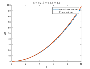
Example 1.

Let us consider the following power fractional equation:

$${}^{p}{}^{C}\!D_{0,t,\omega}^{\alpha,\beta,p}y(t)=t^{2},\quad t\in[0,10]$$ (21)

subject to

$$y(0)=0,$$ (22)

where $\omega(t)\equiv 1$. By applying the power fractional integral to both sides of (21) and using formula $(ii)$ of Theorem 2, we obtain the exact solution of (21)–(22), which is given by

$$y(t)=\phi(\alpha)t^{2}+\frac{2\ln p\cdot\psi(\alpha)}{\Gamma(\beta+3)}t^{\beta+2}.$$ (23)

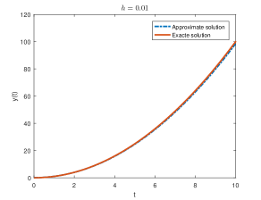
We now apply the developed numerical scheme (19) to approximate the solution of (21)–(22). For numerical simulations, we choose the normalization function

$$N(\alpha)=1-\alpha+\dfrac{\alpha}{\Gamma(\alpha)}.$$

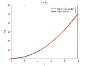
The comparison between the exact and approximate solutions of (21)–(22) is depicted in Figures 1 and 2.

Figure 1: Approximate and exact solutions of system (21)–(22) for $\alpha=0.1$, $\beta=0.2$, $p=1.1$ and different values of the discretization step $h$.

Figure 2: Approximate and exact solutions of system (21)–(22) for different values of $\alpha$, $\beta$ and $p$, with $h=0.001$.

The maximum error of the numerical approximations is given in Table 1, for $\alpha=0.1$, $\beta=0.2$, $p=1.1$ and different values of the discretization step $h$.

Table 1: Maximum error corresponding to different values of $h$ with $\alpha=0.1$, $\beta=0.2$ and $p=1.1$.

Discretization step ($h$)	Approximation error
$h=0.1$	$2.447\times 10^{-1}$
$h=0.01$	$2.080\times 10^{-2}$
$h=0.001$	$6.100\times 10^{-3}$

From Figures 1 and 2, we observe that the proposed numerical method gives a good agreement between the exact and approximate solutions for different value of $\alpha$, $\beta$, $p$ and the discretization step $h$. Table 1 shows that the convergence of the numerical approximation depends on the step of discretization $h$. By comparing the exact and approximate solutions, we conclude that the new proposed numerical scheme is very efficient and converges quickly to the exact solution.

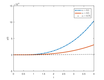
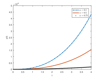
Example 2.

Consider the following nonlinear power fractional differential equation:

$${}^{p}{}^{C}\!D_{0,t,\omega}^{\alpha,1,e}y(t)=\dfrac{t^{2}}{15}\left(\dfrac{\cos(2t)}{1+|y(t)|}\right),\quad t\in[0,4]$$ (24)

subject to

$$y(0)=\sqrt{\pi}.$$ (25)

This example is a particular case of problem (7)–(8) with $\beta=1$, $p=e$, $y_{0}=\sqrt{\pi}$, $a=0$, $b=4$ and

$$f(t,y(t))=\dfrac{t^{2}}{15}\left(\dfrac{\cos(2t)}{1+|y(t)|}\right)$$

with $f(0,y(0))=0$. Here, we choose the normalization function $N(\alpha)=1$.

For all $y,z\in\mathbb{R}$ and $t\in[0,4]$, one has

$$\begin{split}|f(t,y)-f(t,z)|&=\dfrac{t^{2}}{15}|\cos(3t^{2})|\left(\mid\dfrac{1}{1+|y|}-\dfrac{1}{1+|z|}\mid\right)\\ &\leq\dfrac{1}{15}\left(|z|-|y|\right)\\ &\leq\dfrac{1}{15}|y-z|.\end{split}$$

Thus, function $f$ is continuous and satisfies the Lipschitz condition (10) with $L=\dfrac{1}{15}$. Moreover, for any $\alpha\in[0,1)$, we have $\phi(\alpha)=1-\alpha$, $\psi(\alpha)=\alpha$ and

$$L\left(\phi(\alpha)+\dfrac{\ln p\cdot\psi(\alpha)(b-a)^{\beta}}{\Gamma(\beta+1)}\right)=\dfrac{1}{15}\left(1+3\alpha\right)<1.$$

Hence, condition (11) holds. Then, by applying Theorem 4, it follows that problem (24)–(25) has a unique solution on $[0,4]$.

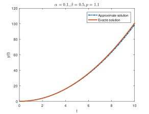
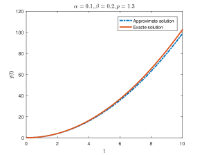
We now use our proposed method to solve the system (24)–(25). For numerical simulations, we take the weight function $\omega(t)=t+2$.

The approximate solution of (24)–(25) is displayed in Figures 3 and 4 for different values of $\alpha$, $\beta=1$ and $p=e$, using two discretization steps: $h=0.1$ and $h=0.01$.

Figure 3: Approximate solution of system (24)–(25) for different values of $\alpha$, $\beta=1$, $p=e$ and $h=0.1$.

Figure 4: Approximate solution of system (24)–(25) for different values of $\alpha$, $\beta=1$, $p=e$ and $h=0.01$.

8 Conclusion

In this paper, (i) we established a new formula for the power fractional derivative with a non-local and non-singular kernel in the form of an infinite series of the standard weighted Riemann–Liouville fractional integral. This brings out more clearly the non-locality properties of the fractional derivative and makes it easier to handle certain computational aspects. By means of the proposed formula, we derived useful properties of the power fractional operators, for example the Newton–Leibniz formula has been rigorously extended. (ii) We presented a new version of Gronwall’s inequality via the power fractional integral, which includes many versions of Gronwall’s inequality found in the literature, such us the generalized Hattaf and Atangana–Baleanu fractional Gronwall’s inequalities. (iii) We proved the existence and uniqueness of solutions to nonlinear power fractional differential equations using the fixed point principle; and, based on Lagrange polynomial interpolation, (iv) we provided a new explicit numerical method to approximate the solutions of power FDEs with the approximation error being also examined. However, we only presented a bound for the error and the proof of the convergence of the numerical scheme is still an open problem. Numerical examples and simulation results were discussed and show that our developed method is very efficient, highly accurate, and converges quickly.

As future work, we aim to apply our obtained analytical and numerical results to develop power fractional models describing real world phenomena such us the world population growth and the dynamics of an epidemic disease. This issue is currently under investigation and will appear elsewhere.

References

• [1] M. Al-Refai, On weighted Atangana-Baleanu fractional operators, Adv. Difference Equ. 2020, Paper No. 3, 11 pp.
• [2] M. Al-Refai and A. M. Jarrah, Fundamental results on weighted Caputo-Fabrizio fractional derivative, Chaos Solitons Fractals 126 (2019), 7–11.
• [3] J. Alzabut, T. Abdeljawad, F. Jarad and W. Sudsutad, A Gronwall inequality via the generalized proportional fractional derivative with applications, J. Inequal. Appl. 2019, Paper No. 101, 12 pp.
• [4] G. A. Anastassiou and I. K. Argyros, Functional numerical methods: applications to abstract fractional calculus, Studies in Systems, Decision and Control, 130, Springer, Cham, 2018.
• [5] A. Atangana  and  D. Baleanu, New fractional derivatives with non-local and non-singular kernel: Theory and application to heat transfer model, Therm. Sci. 20 (2016), no. 2, 763–769.
• [6] D. Baleanu, K. Diethelm, E. Scalas  and J. J. Trujillo, Fractional calculus, Series on Complexity, Nonlinearity and Chaos, 3, World Scientific Publishing Co. Pte. Ltd., Hackensack, NJ, 2012.
• [7] D. Baleanu and A. Fernandez, On some new properties of fractional derivatives with Mittag-Leffler kernel, Commun. Nonlinear Sci. Numer. Simul. 59 (2018), 444–462.
• [8] M. Caputo and M. Fabrizio, A new definition of fractional derivative without singular kernel, Progr. Fract. Differ. Appl. 1 (2015), no. 2, 73–85.
• [9] K. R. Cheneke, K. Purnachandra Rao and G. Kenassa Edessa, Application of a new generalized fractional derivative and rank of control measures on cholera transmission dynamics, Int. J. Math. Math. Sci. 2021 (2021), Art. ID 2104051, 9 pp.
• [10] K. Hattaf, A new generalized definition of fractional derivative with non-singular kernel, Computation 8 (2020), no. 2, Paper No. 49, 9 pp.
• [11] K. Hattaf, On some properties of the new generalized fractional derivative with non-singular kernel, Math. Probl. Eng. 2021, Art. ID 1580396, 6 pp.
• [12] K. Hattaf, On the stability and numerical scheme of fractional differential equations with application to Biology, Computation 10 (2022), no. 6, Paper No. 97, 12 pp.
• [13] K. Hattaf, Z. Hajhouji, M. A. Ichou and N. Yousfi, A numerical method for fractional differential equations with new generalized Hattaf fractional derivative, Mathematical Problems in Engineering 2022 (2022), Article ID 3358071, 9 pp.
• [14] K. Hattaf, A. A. Mohsen and H. F. Al-Husseinye, Gronwall inequality and existence of solutions for differential equations with generalized Hattaf fractional derivative, J. Math. Computer Sci. 27 (2022), 18–27.
• [15] F. Jarad, T. Abdeljawad and Z. Hammouch, On a class of ordinary differential equations in the frame of Atangana-Baleanu fractional derivative, Chaos Solitons Fractals 117 (2018), 16–20.
• [16] A. A. Kilbas, H. M. Srivastava and J. J. Trujillo, Theory and applications of fractional differential equations, North-Holland Mathematics Studies, 204, Elsevier Science B.V., Amsterdam, 2006.
• [17] E. M. Lotfi, H. Zine, D. F. M. Torres and N. Yousfi, The power fractional calculus: First definitions and properties with applications to power fractional differential equations, Mathematics 10 (2022), no. 19, Art. 3594, 10 pp.
• [18] T. R. Prabhakar, A singular integral equation with a generalized Mittag Leffler function in the kernel, Yokohama Math. J. 19 (1971), 7–15.
• [19] T. O. Salim, Some properties relating to the generalized Mittag-Leffler function, Adv. Appl. Math. Anal. 4 (2009), 21–30.
• [20] N. Sene, SIR epidemic model with Mittag-Leffler fractional derivative, Chaos Solitons Fractals 137 (2020), 109833, 9 pp.
• [21] B. Shiri, G.-C. Wu and D. Baleanu, Collocation methods for terminal value problems of tempered fractional differential equations, Appl. Numer. Math. 156 (2020), 385–395.
• [22] H. M. Srivastava  and K. M. Saad, Some new models of the time-fractional gas dynamics equation, Adv. Math. Models Appl. 3 (2018), 5–17.
• [23] M. Toufik  and A. Atangana, New numerical approximation of fractional derivative with non-local and non-singular kernel: Application to chaotic models, European Physical Journal Plus 132 (2017), no. 10, Paper No. 444, 16 pp.
• [24] A. Wiman, $\ddot{U}$ber den fundamental satz in der theorie der functionen $E_{\alpha}(x)$, Acta Mathematica 29 (1905), 191–201.