Multi-fidelity uncertainty quantification for homogenization problems in structure-property relationships from crystal plasticity finite elements

Abstract

Crystal plasticity finite element method (CPFEM) has been an integrated computational materials engineering (ICME) workhorse to study materials behaviors and structure-property relationships for the last few decades. These relations are mappings from the microstructure space to the materials properties space. Due to the stochastic and random nature of microstructures, there is always some uncertainty associated with materials properties, for example, in homogenized stress-strain curves. For critical applications with strong reliability needs, it is often desirable to quantify the microstructure-induced uncertainty in the context of structure-property relationships. However, this uncertainty quantification (UQ) problem often incurs a large computational cost because many statistically equivalent representative volume elements (SERVEs) are needed. In this paper, we apply a multi-level Monte Carlo (MLMC) method to CPFEM to study the uncertainty in stress-strain curves, given an ensemble of SERVEs at multiple mesh resolutions. By using the information at coarse meshes, we show that it is possible to approximate the response at fine meshes with a much reduced computational cost. We focus on problems where the model output is multi-dimensional, which requires us to track multiple quantities of interest (QoIs) at the same time. Our numerical results show that MLMC can accelerate UQ tasks around 2.23$\displaystyle\times$, compared to the classical Monte Carlo (MC) method, which is widely known as ensemble average in the CPFEM literature.

1 Introduction

Designing materials with tailored properties requires a comprehensive understanding of the composition–process–structure–property relationship olson1997computational ; arroyave2019systems , which has been studied extensively with four paradigms of materials science, namely experimental, theoretical, computational, and (scientific) machine learning hey2009fourth ; agrawal2016perspective . For polycrystalline metals and alloys, the materials design problem can often be formulated as optimization under uncertainty, where uncertainty comes from many sources. Some common epistemic uncertainty source includes observation noise, numerical solver tolerance, approximation error, besides the aleatory uncertainty source, which often manifests in the naturally random microstructure. Unfortunately, the materials design cycle is one of the major computational bottlenecks for transformative technologies arroyave2019systems due to their resource-intensive nature. To accelerate the materials design cycle, computational materials paradigms were developed and implemented in that context, across multiple length-scales and time-scales, with the overarching goal of modeling and simulating experimental and theoretical physics olson1997computational . Over the last few decades, multiple integrated computational materials engineering (ICME) national2008integrated models and simulations have been developed. ICME has become the third paradigm in materials science, the so-called computational paradigm agrawal2016perspective . The Materials Genome Initiative (MGI) national2011materials was created in 2011 in that scientific computing context, with the hope that ICME models can significantly reduce the research and development time and cost by leveraging the computational resource of high-performance computers. With the emerging field of machine learning, the revised MGI de2019new was updated in 2019 to include scientific machine learning (SciML) as the fourth paradigm of materials science hey2009fourth ; agrawal2016perspective .

Uncertainty quantification (UQ) plays several important roles in the materials design problemoden2010computer1 ; oden2010computer2 . First of all, many inverse UQ and optimization tools are used to perform deterministic or statistical ICME model calibration. Second, forward UQ tools are applied to quantify uncertainty associated with calibrated ICME models, in order to establish a reliable, robust, and predictive computing capability for ICME. Third, many UQ tools are currently developed and applied to quantify uncertainty for ICME-based SciML. Last but not least, multi-fidelity approaches also play a crucial role in ICME paradigm with multiple fidelity parameters, such as meshes, numerical integrators, iterative solvers, order of element. Therefore, from this perspective, UQ is naturally immersed in all four paradigms of materials science, from experiments to SciML.

Within the composition-process-structure-property relationship, the microstructure is perhaps most uncertain due to its naturally inherent randomness, which can be associated with the aleatory uncertainty. It is well-known that the final microstructure of an alloy is generated “from a very complex, process-specific, history-dependent sequence of transformation” arroyave2019systems . In this paper, we are concerned with quantifying the microstructure-induced uncertainty from the microstructure to the property space, where microstructures are represented by an ensemble of statistically equivalent representative volume elements (SERVEs) in a hierarchical multi-fidelity manner using crystal plasticity finite element model (CPFEM).

Numerous works have been done for UQ in ICME in the last decades. Some notable works are summarized as follows. Nguyen et al. nguyen2021bayesian employed a Markov chain Monte Carlo to calibrate constitutive models for CPFEM in a Bayesian context. Hasan and Acar hasan2022microstructure developed a microstructure-sensitive design for performance optimization in titanium, aluminum, and galfenol. Tran et al. tran2019quantifying ; tran2022microstructure applied stochastic collocation method, which is composed of generalized polynomial chaos expansion and sparse grid for phase-field simulation tran2019quantifying and CPFEM tran2022microstructure , respectively. Venkatraman et al. venkatraman2023new developed a three-step Bayesian protocol for model calibration and model-form UQ for CPFEM constitutive models in $\displaystyle\alpha+\beta$ titanium alloys. Rixner and Koutsourelakis rixner2022self formulated and developed a probabilistic, data-driven convolutional neural network to actively solve an inverse problem in structure-property linkage. Tran and Wildey tran2020solving applied a data-consistent inversion method butler2018combining ; butler2018convergence to infer a distribution of microstructure features from a distribution of yield stress, where the push-forward density map is consistent with a target yield stress density through a heteroscedastic Gaussian process regression. Tran et al. tran2023multi employed multi-level and multi-index Monte Carlo to estimate effective yield strength and effective Young’s modulus in a hierarchical multi-fidelity manner for a single quantity of interest (QoI). Rodgers et al. rodgers2020three simulated the process-structure with kinetic Monte Carlo mitchell2023parallel and the structure-property with CPFEM to study the effects of common microstructure in additive manufacturing. Tran et al. tran2023high employed an asynchronous parallel Bayesian optimization tran2022aphbo to calibrate phenomenological constitutive models for several materials systems. Ricciardi et al. ricciardi2020uncertainty applied the model discrepancy approach kennedy2001bayesian with Gaussian process using a visco-plastic self-consistent model to quantify uncertainty of homogenized stress-strain curve. Khalil et al. khalil2021modeling also applied an adaptive Metropolis-Hastings Markov chain Monte Carlo to calibrate constitutive models accounting for uncertainty in homogenized materials responses. Ghoreishi et al. ghoreishi2018multi proposed a weighted linear average approaches to combine multiple prediction from Gaussian process regression for homogenized stress-strain response for dual-phase microstructures.

In this paper, we extend our previous work in tran2023multi from a single QoI to multiple QoIs, employing the multi-level Monte Carlo (MLMC) method to quantifying uncertainty in the stress-strain curves for a magnesium alloy. The rest of the paper is organized as follows. In section 2, we describe the MLMC method in the context of CPFEM applications. In section 3, we describe the CPFEM case study for magnesium. Our main numerical results, including a comparison between the MLMC method and the brute-force MC method, are discussed in Section 4. In sections 5 and 6, we discuss our results and formulate a conclusion.

2 Multi-level Monte Carlo for microstructure-induced uncertainty quantification

2.1 Microstructure from a statistical perspective

Given a probability space $\displaystyle(\Omega,\mathcal{A},\mathbb{P})$ and $\displaystyle\omega\in\Omega$, we consider an uncertain microstructure $\displaystyle m(\boldsymbol{x},\omega)$ defined on a bounded domain $\displaystyle D\subset\mathbb{R}^{d}$, with $\displaystyle d=2$ or $\displaystyle d=3$. The notation $\displaystyle m(\boldsymbol{x},\omega)$ entails that the microstructure depends on both the spatial variable $\displaystyle\boldsymbol{x}\in D$ as well as the stochastic sample $\displaystyle\omega$ from the sample space of the corresponding probability space. For a fixed $\displaystyle\omega$, the microstructure $\displaystyle m(\boldsymbol{x},\cdot)$ is a deterministic but space-dependent function. For a fixed location $\displaystyle\boldsymbol{x}$, the microstructure $\displaystyle m(\cdot,\omega)$ is a random variable. We are interested in computing statistics of a certain QoI $\displaystyle Q$ that is defined by a mapping $\displaystyle f$ from the microstructure space to the homogenized material property, i.e., $\displaystyle Q=f(m(\cdot,\omega))$. $\displaystyle m(\boldsymbol{x},\omega)$ is often known as the statistically equivalent representative volume element (SERVE) in the materials science literature, sampled independently and identically (i.i.d.) from statistical microstructure measure $\displaystyle\mathbb{P}(\omega)$ that describes all statistical microstructure descriptors, including shape, size, morphology, neighboring, chord length, and crystal orientation distribution functions.

For the remainder of this paper, we will be interested in computing the first-order moment or expected value of the QoI $\displaystyle Q(m)$, defined as

$${\mathbb{E}\left[Q\right]}\coloneqq\int_{\Omega}Q(m(\cdot,\omega))\mathrm{d}\mathbb{P}(\omega).$$ (1)

Since the microstructure $\displaystyle m(\cdot,\omega)$ is not directly accessible, the QoI is often approximated by the quantity $\displaystyle Q_{L}=f(m_{L}(\cdot,\omega))$, where $\displaystyle m_{L}$ is a finite-dimensional approximation to the microstructure $\displaystyle m$ at a particular mesh resolution level $\displaystyle L$, typically the solution of a microstructure reconstruction problem. For readers interested in statistical microstructure descriptors and microstructure reconstruction problems, we refer to some notable works in the literature, for example, groeber2008framework1 ; groeber2008framework2 ; torquato2002statistical ; bostanabad2018computational .

2.2 Monte Carlo method

Given an ensemble of microstructure of $\displaystyle N$ SERVEs, denoted as $\displaystyle\{m(\cdot,\omega^{(n)})\}_{n=1}^{N}$ with corresponding predictions for the material property of interest $\displaystyle\{Q_{L}(m(\cdot,\omega^{(n)}))\}_{n=1}^{N}$ where $\displaystyle Q_{L}$ is the map from microstructure to properties (i.e. a CPFEM simulation), we can approximate Equation (1) by the average

$${\mathcal{Q}}_{\text{MC}}\coloneqq\frac{1}{N}\sum_{n=1}^{N}Q_{L}(m(\cdot,\omega^{(n)})),$$ (2)

where the SERVE $\displaystyle m(\cdot,\omega)$ is sampled from the measure $\displaystyle\mathbb{P}(\omega)$, i.e. $\displaystyle\omega\sim\mathbb{P}(\omega)$. The ensemble average approach in Equation (2), also known as the Monte Carlo (MC) method, is widely used in the CPFEM literature, see, e.g., paulson2017reduced ; teferra2018random ; paulson2018data . For each microstructure SERVE $\displaystyle m(\cdot,\omega^{(n)})$, CPFEM is deployed to evaluate the corresponding material property $\displaystyle Q_{L}(m(\cdot,\omega^{(n)}))$.

It is natural to propose the average of an ensemble of material properties extracted from the microstructures $\displaystyle\{m(\cdot,\omega^{(n)})\}_{n=1}^{N}$ to approximate the expected value in Equation (1). Since the sequence of microstructure SERVEs are drawn from the same underlying sample space $\displaystyle\Omega$ with probability $\displaystyle\mathbb{P}(\omega)$, we have that the expected value $\displaystyle{\mathbb{E}}[Q_{L}(m^{(1)})]=\dots={\mathbb{E}}[Q_{L}(m^{(N)})]={\mathbb{E}}[Q_{L}]$, and the strong law of large numbers guarantees that $\displaystyle{\mathcal{Q}}_{\text{MC}}\to{\mathbb{E}\left[Q_{L}\right]}$ almost surely as the number of microstructure realizations (i.e. the number of SERVE) $\displaystyle N$ goes to infinity, see robert2013monte .

There are two sources of error in the MC estimator in Equation (2): a stochastic error, present because we approximate the expected value by an average, and a bias, present because samples of $\displaystyle Q(m)$ are approximated by samples of $\displaystyle Q_{L}(m)$. The mean square error (MSE) of the estimator can be decomposed into to the sum of these two terms:

$$\begin{array}[]{ll}{\text{MSE}\left({\mathcal{Q}}_{\text{MC}}\right)}&\coloneqq{\mathbb{E}\left[({\mathcal{Q}}_{\text{MC}}-{\mathbb{E}\left[Q\right]})^{2}\right]}\\ &={\mathbb{E}\left[(({\mathcal{Q}}_{\text{MC}}-{\mathbb{E}\left[{\mathcal{Q}}_{\text{MC}}\right]})+({\mathbb{E}\left[{\mathcal{Q}}_{\text{MC}}\right]}-{\mathbb{E}\left[Q\right]}))^{2}\right]}\\ &={\mathbb{E}\left[({\mathcal{Q}}_{\text{MC}}-{\mathbb{E}\left[{\mathcal{Q}}_{\text{MC}}\right]})^{2}\right]}+({\mathbb{E}\left[Q_{L}-Q\right]})^{2}\\ &={\mathbb{V}\left[{\mathcal{Q}}_{\text{MC}}\right]}+({\mathbb{E}\left[Q_{L}-Q\right]})^{2},\end{array}$$ (3)

where the cross-product term vanishes because the MC estimator is an unbiased estimator for $\displaystyle Q_{L}$, i.e., $\displaystyle{\mathbb{E}\left[{\mathcal{Q}}_{\text{MC}}\right]}={\mathbb{E}\left[Q_{L}\right]}$. The first term in Equation (3) is the variance of the estimator and represents the stochastic error. Because we assume the ensemble is uncorrelated, the variance can be written as

$${\mathbb{V}\left[{\mathcal{Q}}_{\text{MC}}\right]}=\frac{1}{N^{2}}\sum_{n=1}^{N}{\mathbb{V}\left[Q_{L}\right]}=\frac{{\mathbb{V}\left[Q_{L}\right]}}{N}.$$ (4)

The variance for the MC estimator $\displaystyle{\mathbb{V}\left[{\mathcal{Q}}_{\text{MC}}\right]}$ decays as $\displaystyle{\mathcal{O}}(N^{-1})$ and can be reduced by considering more SERVEs, i.e. increasing $\displaystyle N$. The second term in Equation (3) is the square of the bias. It can be reduced by increasing the level of resolution $\displaystyle L$, i.e., by decreasing the mesh size, which leads to the notion of $\displaystyle h$-convergence in FEM babuvska1990p .

If we restrict the MSE to be less than or equal to $\displaystyle\epsilon^{2}$, then a sufficient condition could be

$$\frac{{\mathbb{V}\left[Q_{L}\right]}}{N}\leq\frac{\epsilon^{2}}{2}\quad\text{and}\quad|{\mathbb{E}\left[Q_{L}-Q\right]}|\leq\frac{\epsilon}{\sqrt{2}}.$$ (5)

Hence, the number of microstructure SERVEs $\displaystyle N$ scales as $\displaystyle{\mathcal{O}}(\epsilon^{-2})$. Let $\displaystyle C_{L}$ be the cost of a single model evaluation, the total computational cost of the MC estimator in Equation (2) can be expressed as

$$\mathrm{cost}({\mathcal{Q}}_{\text{MC}})=NC_{L}.$$ (6)

Since $\displaystyle C_{L}$ is considered as a constant, the cost complexity of the MC estimator $\displaystyle\mathrm{cost}({\mathcal{Q}}_{\text{MC}})$ is the same as the number of SERVEs, i.e. $\displaystyle N$ $\displaystyle{\mathcal{O}}(\epsilon^{-2})$.

2.3 Multi-level Monte Carlo

The main idea of MLMC sampling giles2015multilevel is that instead of sampling from only one approximation $\displaystyle Q_{L}$, we sample from a hierarchy of approximation $\displaystyle\{Q_{\ell}\}_{\ell=0}^{L}$ for the QoI, denoted as $\displaystyle Q$. $\displaystyle\ell=0$ indicates the lowest level of fidelity and $\displaystyle\ell=L$ indicates the highest level of fidelity. From the multi-fidelity perspective, the intuition is to approximate the high-fidelity data using low-fidelity data by their correlation and hopefully, reducing the computational cost while retaining the approximation accuracy. In the context of this paper, $\displaystyle\ell=0$ corresponds to the coarsest mesh size and $\displaystyle\ell=L$ corresponds to the finest mesh size, respectively, and $\displaystyle\{Q_{\ell}\}_{\ell=0}^{L}$ is a sequence of meshes.

Thanks to the linear property of the expectation operator, we can decompose the expectation at the highest level of fidelity into a telescoping sum as

$${\mathbb{E}\left[Q_{L}\right]}={\mathbb{E}\left[Q_{0}\right]}+\sum_{\ell=1}^{L}{\mathbb{E}\left[Q_{\ell}-Q_{\ell-1}\right]}=\sum_{\ell=0}^{L}{\mathbb{E}\left[\Delta Q_{\ell}\right]}$$ (7)

where the backward difference is

$$\Delta Q_{\ell}\coloneqq\begin{cases}Q_{\ell}-Q_{\ell-1},&\text{for }\ell>0,\\ Q_{\ell},&\text{for }\ell=0.\\ \end{cases}$$ (8)

Using the MC estimator to estimate $\displaystyle{\mathbb{E}\left[\Delta Q_{\ell}\right]}$ for $\displaystyle 0\leq\ell\leq L$, the MLMC estimator can be written as

$${\mathcal{Q}}_{\text{MLMC}}\coloneqq\sum_{\ell=0}^{L}\frac{1}{N_{\ell}}\sum_{n=1}^{N_{\ell}}\Delta Q_{\ell}(m(\cdot,\omega^{(n)})).$$ (9)

Theoretically, this means an ensemble of microstructure SERVEs $\displaystyle\{m^{(n)}\}_{n=1}^{N_{\ell}}$ is used to estimate $\displaystyle\Delta Q_{\ell}$ from the telescoping sum in Equation (7), for $\displaystyle 0\leq\ell\leq L$.

The MLMC estimator in Equation (9) is still an unbiased estimator for $\displaystyle{\mathbb{E}\left[Q_{L}\right]}$, i.e., $\displaystyle{\mathbb{E}\left[{\mathcal{Q}}_{\text{MLMC}}\right]}={\mathbb{E}\left[\Delta Q_{L}\right]}$ with variance

$${\mathbb{V}\left[{\mathcal{Q}}_{\text{MLMC}}\right]}=\sum_{\ell=0}^{L}\frac{{\mathbb{V}\left[\Delta Q_{\ell}\right]}}{N_{\ell}}.$$ (10)

Decomposing the MSE into the bias and variance as in (3), we have

$${\text{MSE}\left({\mathcal{Q}}_{\text{MLMC}}\right)}={\mathbb{V}\left[{\mathcal{Q}}_{\text{MLMC}}\right]}+({\mathbb{E}\left[Q_{L}-Q\right]})^{2}=\sum_{\ell=0}^{L}\frac{{\mathbb{V}\left[\Delta Q_{\ell}\right]}}{N_{\ell}}+({\mathbb{E}\left[Q_{L}-Q\right]})^{2}.$$ (11)

It is worthy to point out that the bias of the MLMC estimator is the same as the bias of the MC estimator.

If the $\displaystyle Q_{\ell}$ and $\displaystyle Q_{\ell-1}$ are strongly positively correlated, then

$$\begin{array}[]{lll}{\mathbb{V}\left[\Delta Q_{\ell}\right]}&={\mathbb{V}}[Q_{\ell}-Q_{\ell-1}]\\ &={\mathbb{V}\left[Q_{\ell}\right]}+{\mathbb{V}\left[Q_{\ell-1}\right]}-2\text{cov}(Q_{\ell},Q_{\ell-1})\\ &\ll{\mathbb{V}\left[Q_{\ell}\right]}+{\mathbb{V}\left[Q_{\ell-1}\right]},\end{array}$$ (12)

where $\displaystyle\text{cov}(Q_{\ell},Q_{\ell-1})=\rho_{\ell,\ell-1}\sqrt{{\mathbb{V}\left[Q_{\ell}\right]}{\mathbb{V}\left[Q_{\ell-1}\right]}}$ is the covariance between $\displaystyle Q_{\ell}$ and $\displaystyle Q_{\ell-1}$ and $\displaystyle\rho_{\ell,\ell-1}$ is the Pearson correlation coefficient. Notice that the backward difference $\displaystyle{\mathbb{E}\left[\Delta Q_{\ell}\right]}$ is computed on the same input microstructure $\displaystyle m(\cdot,\omega^{(n)})$. As $\displaystyle\ell\rightarrow\infty$, we recover the $\displaystyle h$-convergence from the asymptotic analysis of FEM when the mesh size approaches zero, i.e. $\displaystyle h\to 0$.

If we require an MSE smaller than or equal to $\displaystyle\epsilon^{2}$, a sufficient condition is

$$\sum_{\ell=0}^{L}\frac{{\mathbb{V}\left[\Delta Q_{\ell}\right]}}{N_{\ell}}\leq\frac{\epsilon^{2}}{2}\quad\text{and}\quad|{\mathbb{E}\left[Q_{L}-Q\right]}|\leq\frac{\epsilon}{\sqrt{2}}.$$ (13)

The total cost of the MLMC estimator is

$$\mathrm{cost}({\mathcal{Q}}_{\text{MLMC}})=\sum_{\ell=0}^{L}N_{\ell}\Delta C_{\ell},$$ (14)

where $\displaystyle\Delta C_{\ell}$ is the sampling cost of the backward difference $\displaystyle\Delta Q_{\ell}$. The optimal number of samples is giles2015multilevel

$$N_{\ell}=\frac{2}{\epsilon^{2}}\sqrt{\frac{{\mathbb{V}\left[\Delta Q_{\ell}\right]}}{\Delta C_{\ell}}}\left(\sum_{\ell=0}^{L}\sqrt{{\mathbb{V}\left[\Delta Q_{\ell}\right]}\Delta C_{\ell}}\right),$$ (15)

Numerically, $\displaystyle N_{\ell}$ in (15) is rounded up to the nearest integer, which in turn, may increase the cost of the estimator by at most one sample per level.

Assuming that the expectation, variance, and sampling cost are bounded as

$$\displaystyle|{\mathbb{E}\left[\Delta{\mathcal{Q}}_{\ell}\right]}| \displaystyle\leq c_{1}\;2^{-\alpha\ell},$$ (C1)

$$\displaystyle{\mathbb{V}\left[\Delta{\mathcal{Q}}_{\ell}\right]} \displaystyle\leq c_{2}\;2^{-\beta\ell}\text{ and}$$ (C2)

$$\displaystyle\Delta C_{\ell} \displaystyle\leq c_{3}\;2^{\gamma\ell}$$ (C3)

with $\displaystyle 2\alpha\geq\min(\beta,\gamma)$, the asymptotic cost complexity of the MLMC estimator is cliffe2011multilevel

$${\text{cost}\left({\mathcal{Q}}_{\text{MLMC}}\right)}\leq\begin{cases}c_{4}\;\epsilon^{-2}&\text{if }\beta>\gamma,\\ c_{4}\;\epsilon^{-2}(\log\epsilon)^{2}&\text{if }\beta=\gamma,\\ c_{4}\;\epsilon^{-2-(\gamma-\beta)/\alpha}&\text{if }\beta<\gamma.\end{cases}$$ (16)

The extension of MLMC methods to multi-output MLMC is simply done by imposing the convergence criteria on the $\displaystyle L_{\infty}$ norm of the vector-valued output.

2.4 Integrated workflow: MultilevelEstimators.jl + DREAM.3D + DAMASK

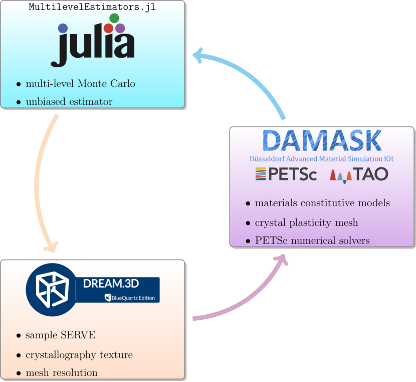
Figure 1: Multi-fidelity uncertainty quantification workflow for CPFEM.

Figure 1 describes the integrated workflow used in this paper. In this workflow, three different software packages are integrated to create a UQ framework for CPFEM problems. At each iteration, MultilevelEstimators.jl robbe2017multi ; robbe2019recycling requests an evaluation of the CPFEM model at fidelity levels $\displaystyle\ell$ and $\displaystyle\ell-1$. DREAM.3D groeber2014dream is then employed to generate a microstructure SERVE on these mesh resolution levels. DAMASK roters2019damask uses the generated microstructure geometries and computes the QoI using a PETSc balay1997efficient ; petsc-web-page backend. The workflow is coupled together using a combination of Python and shell scripts.

3 Crystal plasticity finite element for magnesium

3.1 Phenomenonlogical constitutive model

In this section, we followed  roters2010overview ; roters2011crystal ; roters2019damask to summarize the basic of CPFEM with phenomenological constitutive model. The multiplicative elasto-plastic decomposition of deformation gradient for large deformations reads as

$$\mathbf{F}=\mathbf{F}_{\text{e}}\cdot\mathbf{F}_{\text{p}},$$ (17)

and the elasto-plastic decomposition of the velocity gradient is

$$\mathbf{L}=\dot{\mathbf{F}}\cdot\mathbf{F}^{-1}=\dot{\mathbf{F}}_{\text{e}}\cdot\mathbf{F}_{\text{e}}^{-1}+\mathbf{F}_{\text{e}}\cdot\dot{\mathbf{F}}_{\text{p}}\cdot\mathbf{F}_{\text{p}}\cdot\mathbf{F}_{\text{e}}^{-1}=\mathbf{L}_{\text{e}}+\mathbf{F}_{\text{e}}\cdot\mathbf{L}_{\text{p}}\cdot\mathbf{F}_{\text{e}}^{-1},$$ (18)

$\displaystyle\mathbf{L}_{\text{p}}$ and $\displaystyle\mathbf{L}_{\text{e}}$ are the plastic and elastic velocity gradient, respectively. The flow rules models the evolution of the inelastic deformation gradient $\displaystyle\mathbf{F}_{\text{p}}$ as

$$\displaystyle\dot{\mathbf{F}}_{\text{p}}=\mathbf{L}_{\text{p}}\mathbf{F}_{\text{p}},$$ (19)

where the plasticity velocity gradient in the intermediate configuration $\displaystyle\mathbf{L}_{\text{p}}$ is determined by

$$\mathbf{L}_{\text{p}}=\dot{\mathbf{F}}_{\text{p}}\cdot\mathbf{F}_{\text{p}}^{-1}=\sum_{\alpha}\dot{\gamma}^{\alpha}\left(\mathbf{s}_{\text{s}}^{\alpha}\otimes\mathbf{n}_{\text{s}}^{\alpha}\right).$$ (21)

$\displaystyle\mathbf{s}_{\text{s}}^{\alpha}$ is the unit vector along the slip direction and $\displaystyle\mathbf{n}_{\text{s}}^{\alpha}$ is the unit vectors normal to the slip plane.

Plasticity is considered in terms of resistance $\displaystyle\xi$ on $\displaystyle N_{\text{s}}$ slip and $\displaystyle N_{\text{tw}}$ twin systems. The resistances on $\displaystyle\alpha=1,\dots,N_{\text{s}}$ slip systems evolve as

$$\begin{array}[]{lll}\dot{\xi}^{\alpha}&=&h_{0}^{\text{s-s}}\left(1+c_{1}\left(f^{\text{tot}}_{\text{tw}}\right)^{c_{2}}\right)(1+h^{\alpha}_{\text{int}})\left[\sum_{\alpha^{\prime}=1}^{N_{\text{s}}}|\dot{\gamma}^{\alpha^{\prime}}|\left|1-\frac{\xi^{\alpha^{\prime}}}{\xi^{\alpha^{\prime}}_{\infty}}\right|^{a}\text{sgn}\left(1-\frac{\xi^{\alpha^{\prime}}}{\xi^{\alpha^{\prime}}_{\infty}}\right)h^{\alpha\alpha^{\prime}}\right]\\ &&+\sum_{\beta^{\prime}=1}^{N_{\text{tw}}}\dot{\gamma}^{\beta^{\prime}}h^{\alpha\beta^{\prime}},\end{array}$$ (22)

where $\displaystyle f^{\text{tot}}_{\text{tw}}$ is the total twin volume fraction, $\displaystyle h$ is the matrices of the slip-slip and slip-twin interactions, $\displaystyle h_{0}^{\text{s-s}}$, $\displaystyle h_{\text{int}}$, $\displaystyle c_{1}$, $\displaystyle c_{2}$ are fitting parameters, $\displaystyle\xi_{\infty}$ is the saturated resistance.

The resistances on the $\displaystyle\beta=1,\dots,N_{\text{tw}}$ twin systems evolve similarly:

$$\dot{\xi}^{\beta}=h_{0}^{\text{tw-s}}\left(\sum_{\alpha=1}^{N_{\text{s}}}|\gamma_{\alpha}|\right)^{c_{3}}\left(\sum_{\alpha^{\prime}=1}^{N_{\text{s}}}|\dot{\gamma}^{\alpha^{\prime}}|h^{\beta\alpha^{\prime}}\right)+h_{0}^{\text{tw-tw}}\left(f^{\text{tot}}_{\text{tw}}\right)^{c_{4}}\left(\sum_{\beta^{\prime}=1}^{N_{\text{tw}}}\dot{\gamma}^{\beta^{\prime}}h^{\beta\beta^{\prime}}\right),$$ (23)

where $\displaystyle h_{0}^{\text{tw-s}}$, $\displaystyle h_{0}^{\text{tw-tw}}$, $\displaystyle c_{3}$, and $\displaystyle c_{4}$ are fitting parameters. Shear on each slip system evolves as

$$\dot{\gamma}^{\alpha}=(1-f^{\text{tot}}_{\text{tw}})\dot{\gamma_{0}}^{\alpha}\left|\frac{\tau^{\alpha}}{\xi^{\alpha}}\right|^{n}\text{sgn}(\tau^{\alpha}).$$ (24)

where slip due to mechanical twinning is

$$\dot{\gamma}=(1-f^{\text{tot}}_{\text{tw}})\dot{\gamma_{0}}\left|\frac{\tau}{\xi}\right|^{n}\mathcal{H}(\tau).$$ (25)

$\displaystyle\mathcal{H}$ is the Heaviside step function. The total twin volume is

$$f^{\text{tot}}_{\text{tw}}=\max\left(1.0,\sum_{\beta=1}^{N_{\text{tw}}}\frac{\gamma^{\beta}}{\gamma^{\beta}_{\text{char}}}\right),$$ (26)

where $\displaystyle\gamma_{\text{char}}$ is the characteristic shear due to mechanical twinning and depends on the twin system. Interested readers are referred to the work of Roters et al. roters2010overview for a complete picture of CPFEM model in general and for using DAMASK roters2019damask in particular. Table 1 lists the constitutive parameter used in this example from the literature  sedighiani2020efficient ; sedighiani2022determination ; wang2014situ ; tromans2011elastic ; agnew2006validating .

Table 1: Parameters for Mg used in this case study (cf. Tables 7 and 8 sedighiani2020efficient ; sedighiani2022determination ,  wang2014situ ; tromans2011elastic ; agnew2006validating ).

variable	description	units	reference value
$\displaystyle c/a$	lattice parameter ratio	–	1.635
$\displaystyle C_{11}$	elastic constant	GPa	59.3
$\displaystyle C_{12}$	elastic constant	GPa	61.5
$\displaystyle C_{44}$	elastic constant	GPa	16.4
$\displaystyle C_{44}$	elastic constant	GPa	25.7
$\displaystyle C_{44}$	elastic constant	GPa	21.4
$\displaystyle\dot{\gamma}_{0}$	twinning reference shear rate	s-1	0.001
$\displaystyle\dot{\gamma}_{0}$	slip reference shear rate	s-1	0.001
$\displaystyle\tau_{0,\text{basal}}$	basal slip resistance	MPa	10
$\displaystyle\tau_{0,\text{pris}}$	prismatic slip resistance	MPa	55
$\displaystyle\tau_{0,\text{pyr}\langle a\rangle}$	pyramidal $\displaystyle\langle a\rangle$ slip resistance	MPa	60
$\displaystyle\tau_{0,\text{pyr}\langle c+a\rangle}$	pyramidal $\displaystyle\langle c+a\rangle$ slip resistance	MPa	60
$\displaystyle\tau_{0,\text{T}1}$	tensile twin resistance	MPa	45
$\displaystyle\tau_{0,\text{C}2}$	compressive twin resistance	MPa	80
$\displaystyle\tau_{\infty,\text{basal}}$	basal saturation stress	MPa	45
$\displaystyle\tau_{\infty,\text{pris}}$	prismatic saturation stress	MPa	135
$\displaystyle\tau_{\infty,\text{pyr}\langle a\rangle}$	pyramidal $\displaystyle\langle a\rangle$ saturation stress	MPa	150
$\displaystyle\tau_{\infty,\text{pyr}\langle c+a\rangle}$	pyramidal $\displaystyle\langle c+a\rangle$ saturation stress	MPa	150
$\displaystyle h_{0}^{\text{tw}-\text{tw}}$	twin-twin hardening parameter	MPa	50
$\displaystyle h_{0}^{\text{s}-\text{s}}$	slip-slip hardening parameter	MPa	500
$\displaystyle h_{0}^{\text{tw}-\text{s}}$	twin-slip hardening parameter	MPa	150
$\displaystyle n_{\text{s}}$	slip strain rate sensitivity parameter	–	10
$\displaystyle n_{\text{tw}}$	twinning strain rate sensitivity parameter	–	5
$\displaystyle a$	slip hardening parameter	–	2.5

Table 2: Mesh resolutions and corresponding number of degrees of freedom (i.e. SERVE size) used in this study.

$\displaystyle\ell$	Degrees of freedom	# processors/sample	cost/sample [s]
0	$\displaystyle 2\times 2\times 2$	1	39
1	$\displaystyle 4\times 4\times 4$	1	365
2	$\displaystyle 8\times 8\times 8$	2	1955
3	$\displaystyle 16\times 16\times 16$	4	3305
4	$\displaystyle 32\times 32\times 32$	8	12487

3.2 Crystallography and microstructure for magnesium

Figure 2 presents three different SERVEs with geometric mesh resolution levels chosen as detailed in Table 2. The SERVEs are reconstructed using DREAM.3D, where the grain sizes are log normally distributed with equiaxed grains, i.e. $\displaystyle d\sim\text{LogNormal}(\mu_{d},\sigma_{d})$, $\displaystyle\mu_{d}=5.2983,\sigma_{d}=0.2$. Following mangal2018dataset ; tran2022microstructure , the crystallographic texture for magnesium is sampled from $\displaystyle(\phi_{1},\theta,\phi_{2})=(90^{\circ},0^{\circ},0^{\circ})$ and shown in Figure 3.

(a) $\displaystyle m_{1}:2\times 2\times 2$

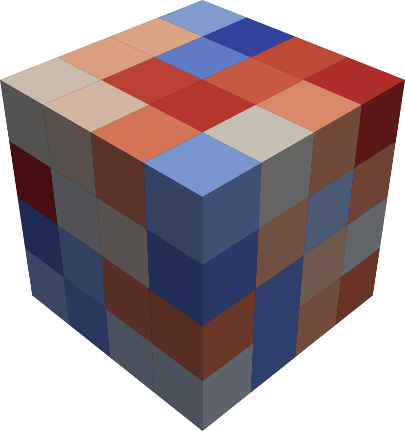
(b) $\displaystyle m_{1}:4\times 4\times 4$

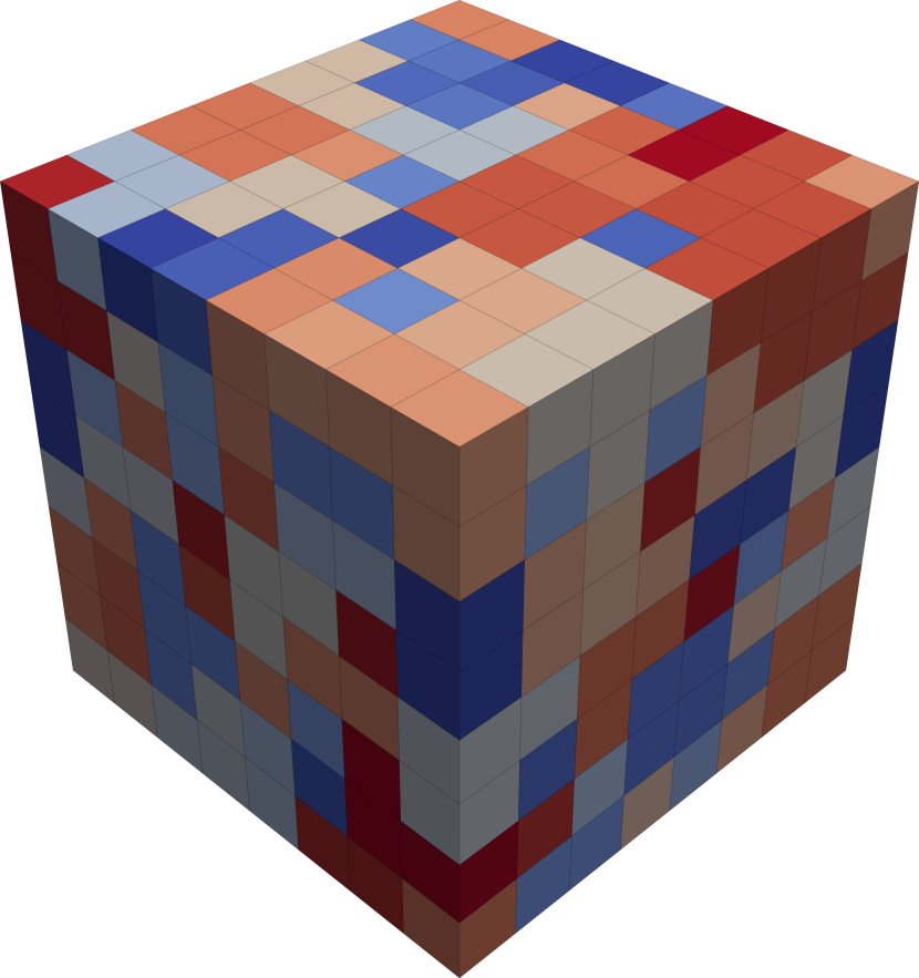
(c) $\displaystyle m_{1}:8\times 8\times 8$

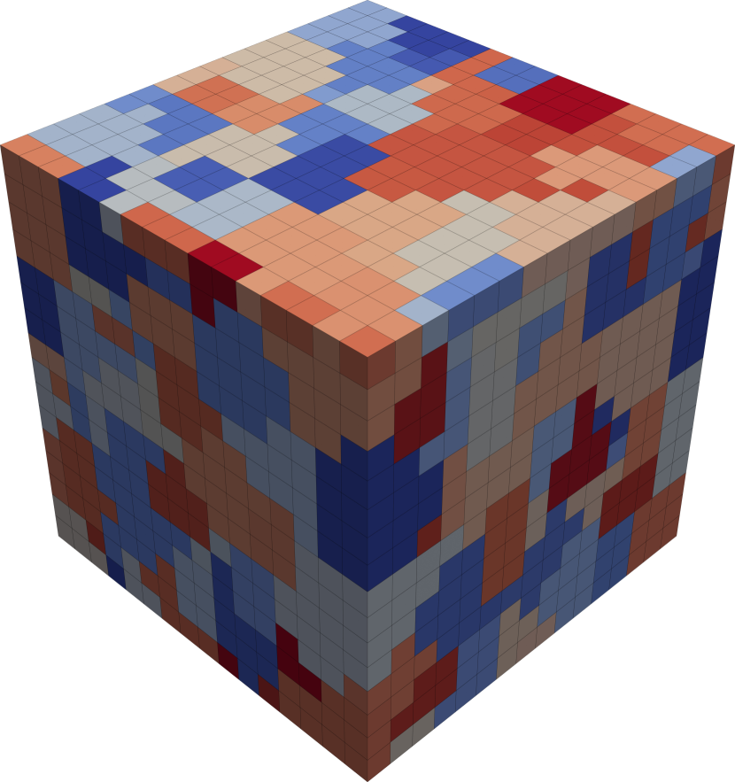
(d) $\displaystyle m_{1}:16\times 16\times 16$

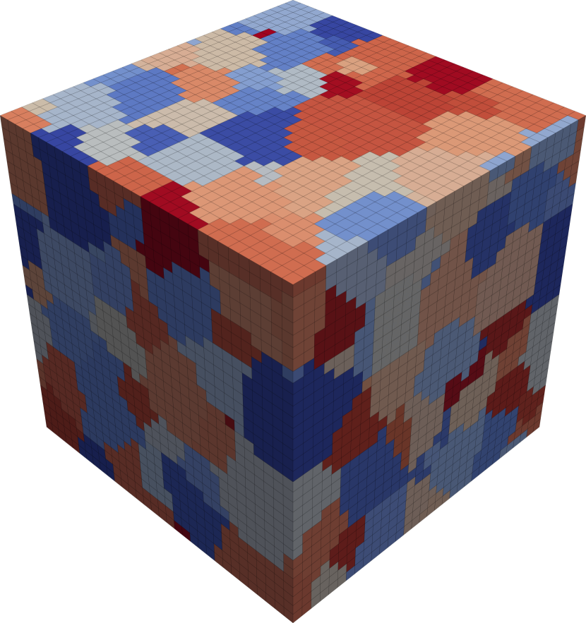
(e) $\displaystyle m_{1}:32\times 32\times 32$

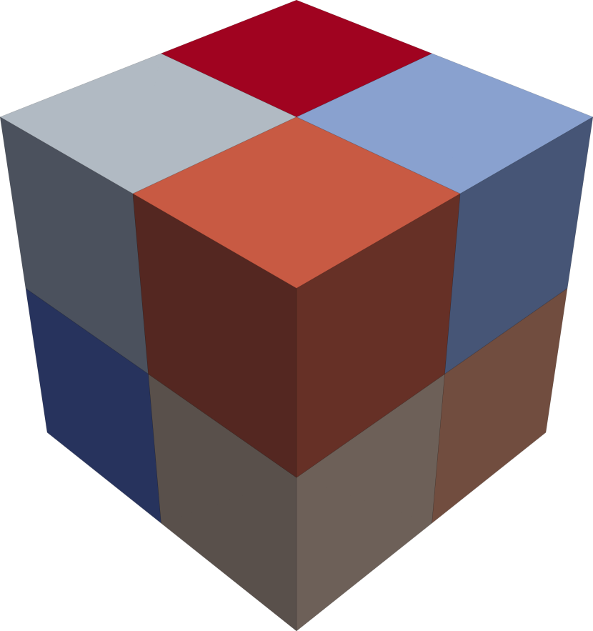
(f) $\displaystyle m_{2}:2\times 2\times 2$

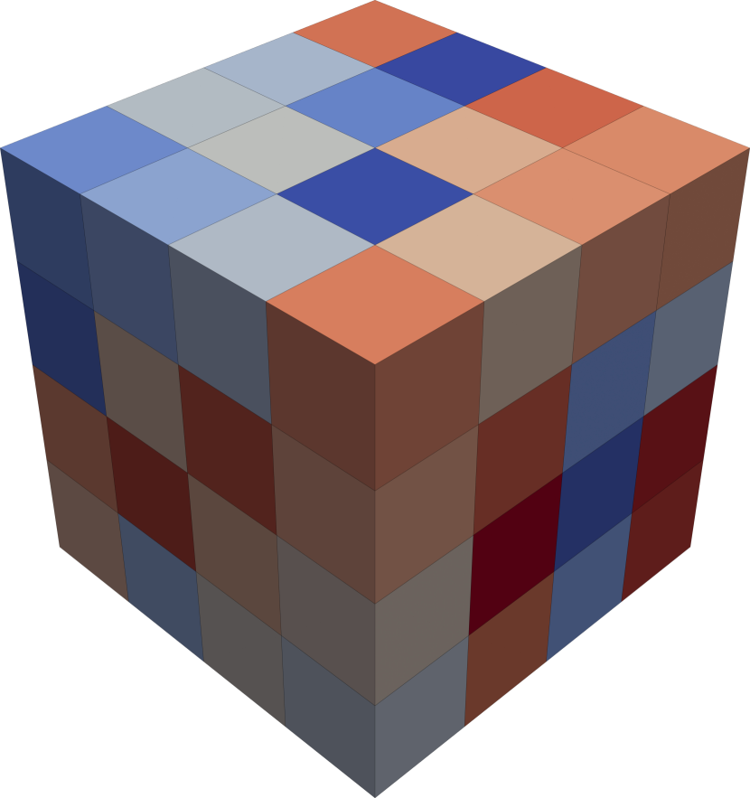
(g) $\displaystyle m_{2}:4\times 4\times 4$

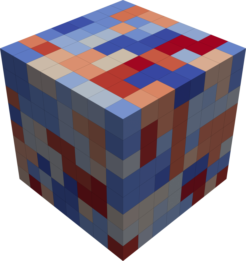
(h) $\displaystyle m_{2}:8\times 8\times 8$

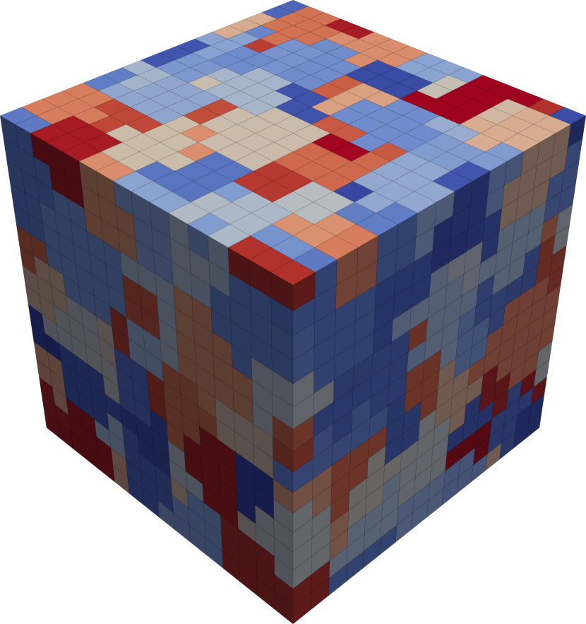
(i) $\displaystyle m_{2}:16\times 16\times 16$

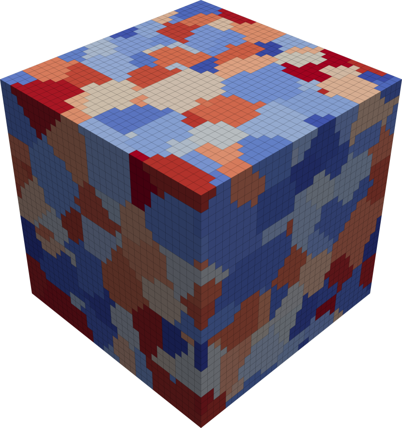
(j) $\displaystyle m_{2}:32\times 32\times 32$

(k) $\displaystyle m_{3}:2\times 2\times 2$

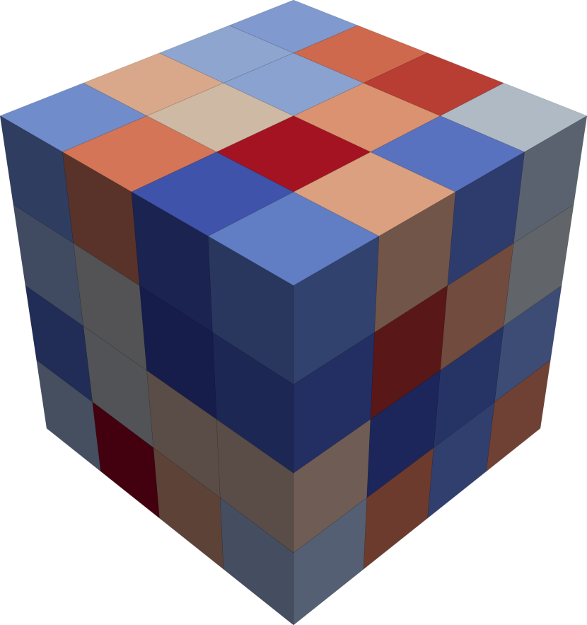
(l) $\displaystyle m_{3}:4\times 4\times 4$

(m) $\displaystyle m_{3}:8\times 8\times 8$

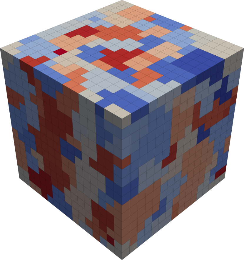
(n) $\displaystyle m_{3}:16\times 16\times 16$

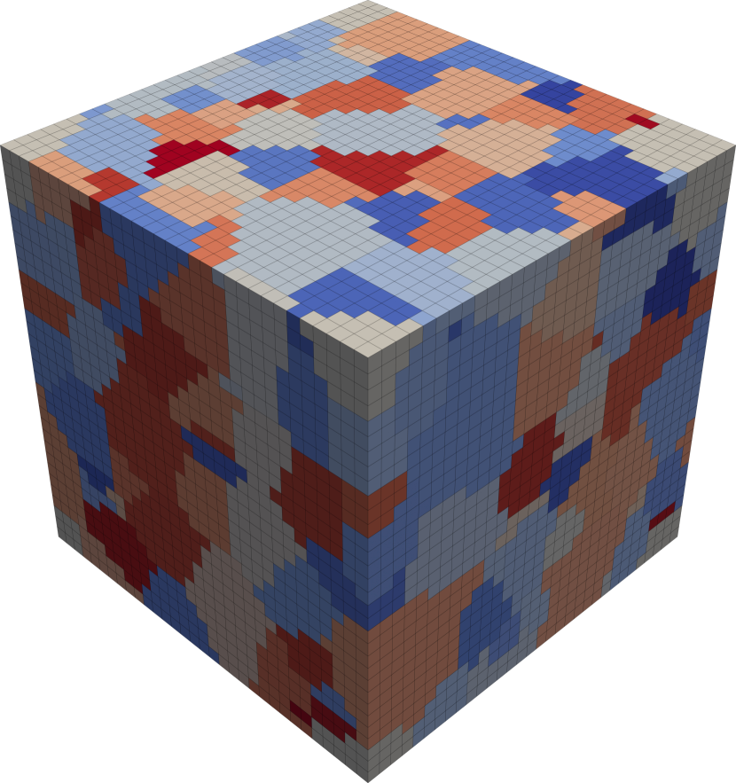
(o) $\displaystyle m_{3}:32\times 32\times 32$

Figure 2: Three SERVE realizations, i.e. $\displaystyle m_{1}$, $\displaystyle m_{2}$, and $\displaystyle m_{3}$, discretized at 5 geometric mesh resolutions: $\displaystyle 2\times 2\times 2$, $\displaystyle 4\times 4\times 4$, $\displaystyle 8\times 8\times 8$, $\displaystyle 16\times 16\times 16$, and $\displaystyle 32\times 32\times 32$.

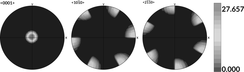
Figure 3: Magnesium texture component with Euler angles $\displaystyle(\phi_{1},\theta,\phi_{2})=(90^{\circ},0^{\circ},0^{\circ})$

.

4 Numerical results

4.1 Problem description

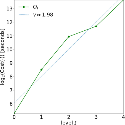
Figure 4: Increase of the average computational cost per sample expressed in seconds as a function of the level parameter $\displaystyle\ell$ using the mesh refinement as a fidelity parameter in the MLMC experiment. The dashed line corresponds to a fit of the computational cost proportional to $\displaystyle 2^{\gamma\ell}$ with $\displaystyle\gamma\approx 1.98$, see condition (C3). The computational cost at each level can be found in Table 2).

In this section, we discuss the setup of our numerical experiments. We are interested in estimating homogenized stress curves for magnesium at different strain levels. We compute those curves using both the MC method and the MLMC method outlined in Section 2. For the MLMC method, we use a geometric mesh resolution level hierarchy as shown in Table 2. Figure 4 shows the increase in computational cost associated with each level, indicating that the cost increases geometrically with the mesh resolution level number. Although the number of degrees of freedom increases with a factor 8 as the mesh resolution level increases, the computational cost scales only as $\displaystyle 2^{\gamma\ell}$, where we numerically fitted $\displaystyle\gamma\approx 1.98$. This is because we use a different number of processors at each level, following a constraint on the number of grid points per processor imposed by DAMASK. The number of processors used for each mesh resolution level is shown in Table 2.

4.2 MLMC estimation of homogenized mean stress-strain responses

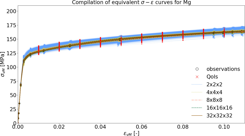
Figure 5: Compilation of stress-strain curves by sampling SERVEs at the different mesh resolution levels shown in Table 2. The locations of the 9 QoIs are plotted as $\displaystyle{\color[rgb]{1,0,0}\times}$.

Figure 5 shows a collection of the stress-strain curve evaluated for an ensemble of SERVEs at each mesh resolution level provided in Table 2. As the fidelity level increases, the mesh becomes finer, and the number of SERVEs decreases. Hence, the plot is dominated by stress-strain curves collected at $\displaystyle 2\times 2\times 2$, and much less at $\displaystyle 32\times 32\times 32$. We interpolate the obtained stress-strain curves at a set of 9 prescribed strain values $\displaystyle\varepsilon=\{0.1,0.2,\ldots,0.9\}$. We use cubic Hermite spline interpolation virtanen2020scipy to obtain the values of the stress-strain curves at those 9 locations. This higher-order interpolation scheme should avoid additional interpolation errors that converge at a slower rate than the bias in the predicted stress-strain curves. The value of the stress-strain curve at those 9 locations will be the set of QoIs we are interested in. Note that these QoIs are indicated by $\displaystyle{\color[rgb]{1,0,0}\times}$in Figure 5.

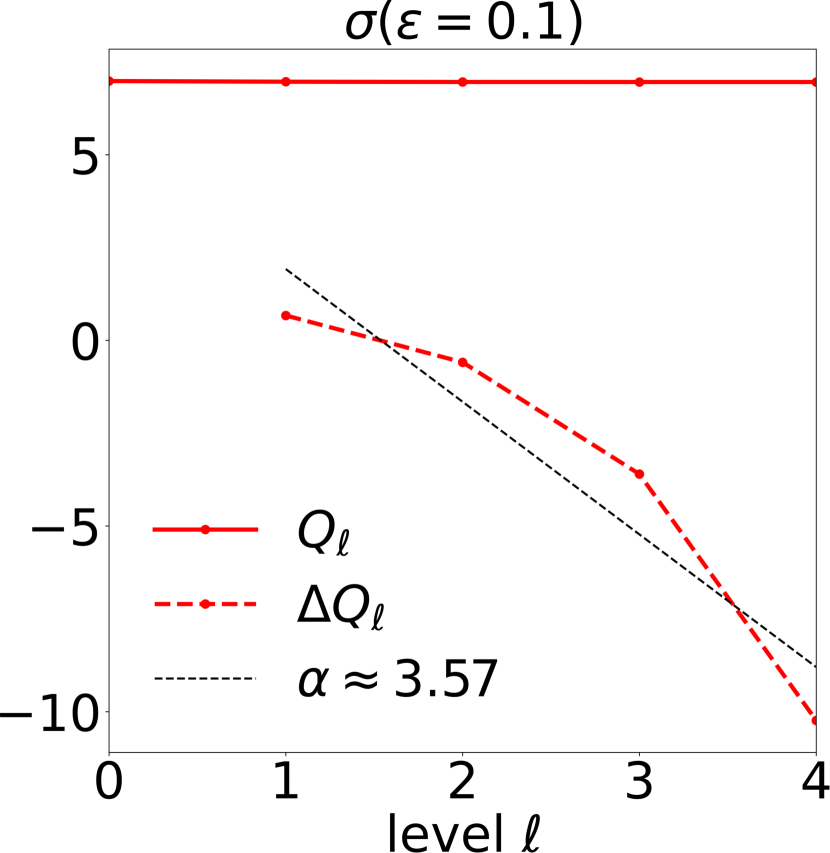
(a) $\displaystyle\varepsilon=0.10$

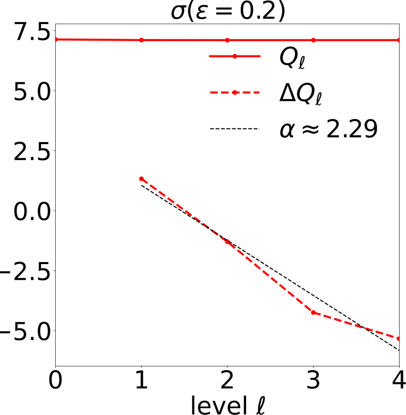
(b) $\displaystyle\varepsilon=0.20$

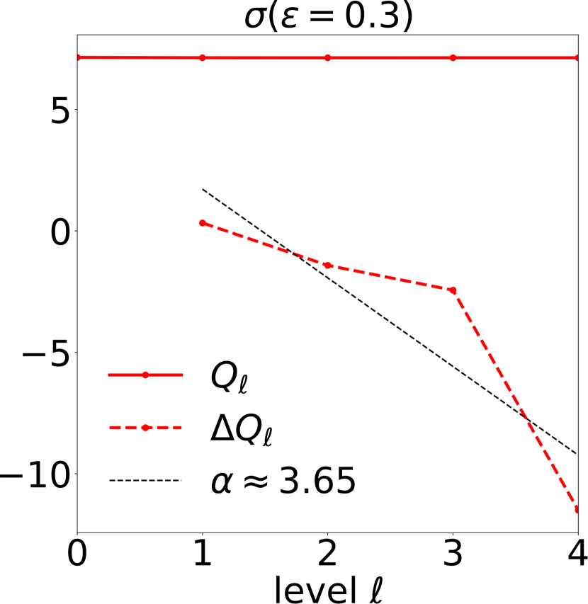
(c) $\displaystyle\varepsilon=0.30$

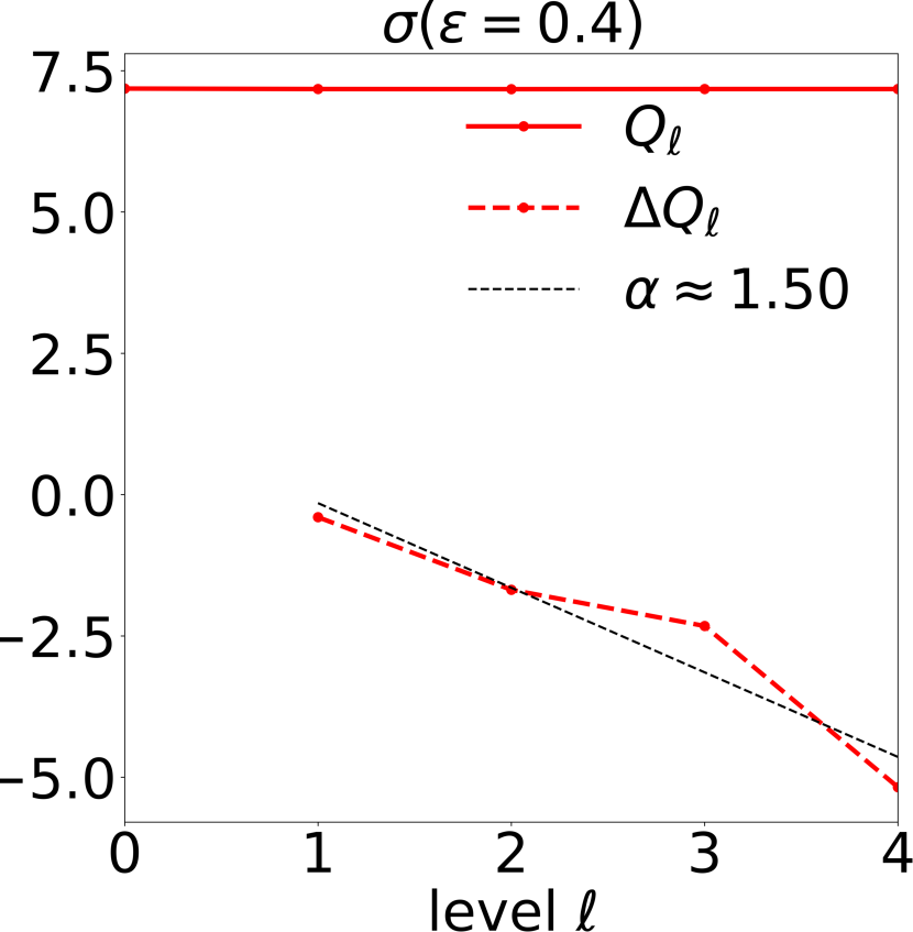
(d) $\displaystyle\varepsilon=0.40$

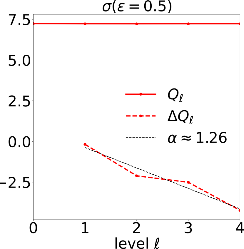
(e) $\displaystyle\varepsilon=0.50$

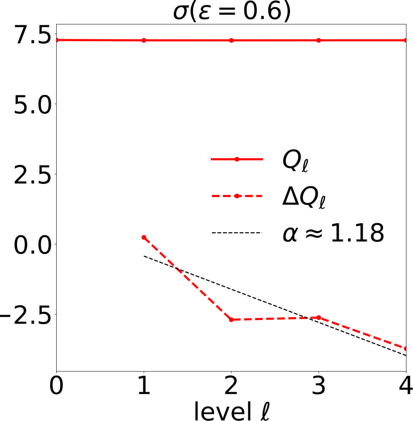
(f) $\displaystyle\varepsilon=0.60$

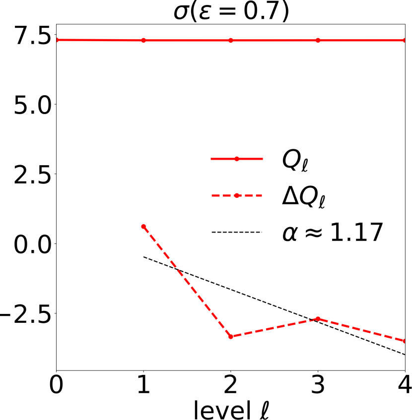
(g) $\displaystyle\varepsilon=0.70$

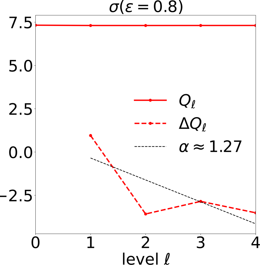
(h) $\displaystyle\varepsilon=0.80$

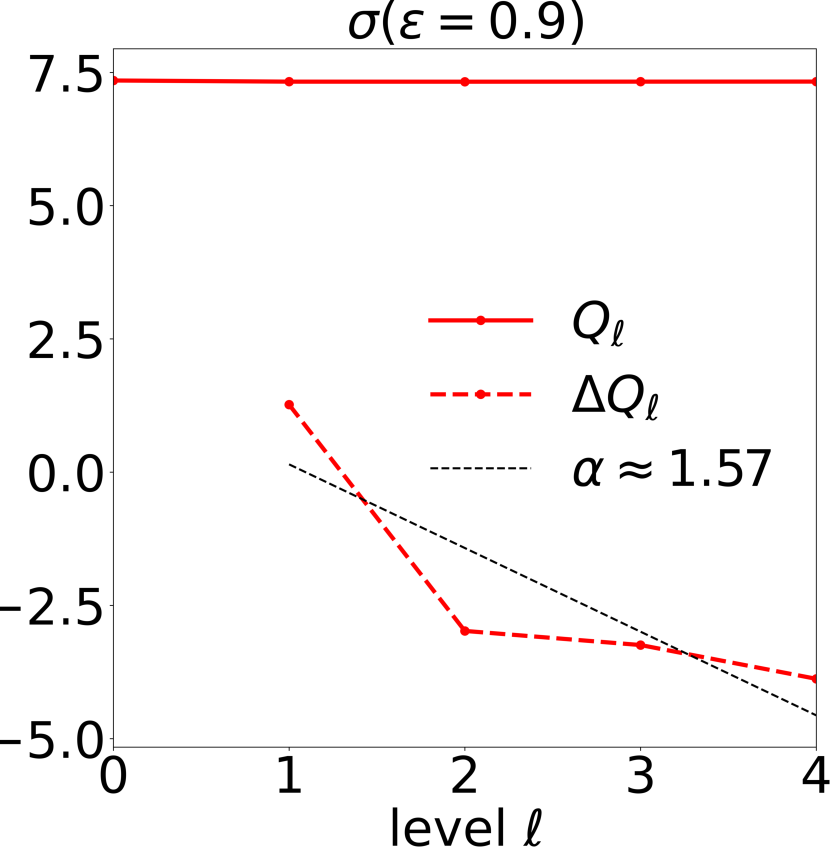
(i) $\displaystyle\varepsilon=0.90$

Figure 6: Behavior of the expected value $\displaystyle\log_{2}(\mathbb{E}[\left|\cdot\right|])$ of the quantities of interest $\displaystyle Q_{\ell}$ and the multi-level difference $\displaystyle\Delta Q_{\ell}$ as a function of the level $\displaystyle\ell$ using the mesh refinement as a fidelity parameter for each QoI. We numerically fitted the values $\displaystyle{\mathbb{E}}[\Delta Q_{\ell}]\;\propto\;2^{-\alpha\ell}$ with $\displaystyle 1.34\lesssim\alpha\lesssim 2.93$, see Table 3.

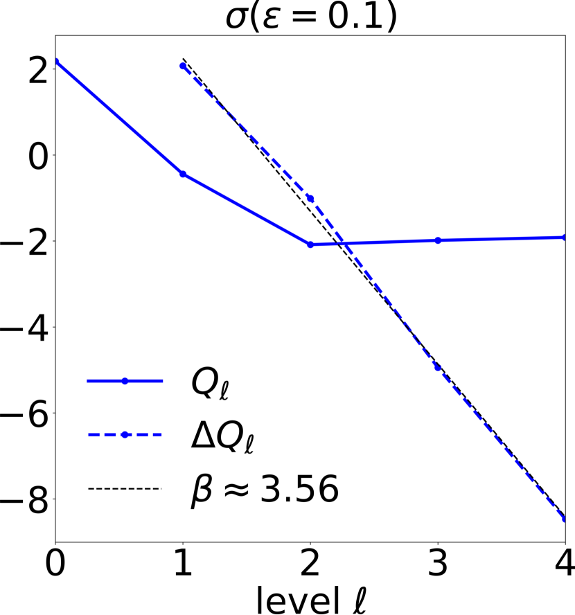
(a) $\displaystyle\varepsilon=0.10$

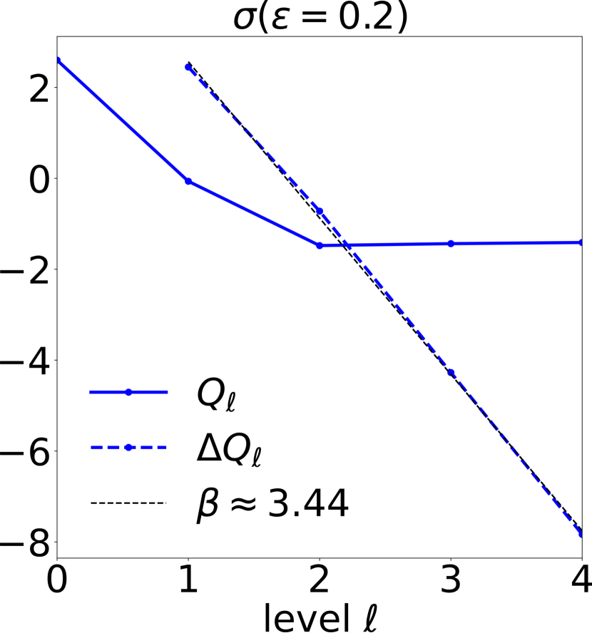
(b) $\displaystyle\varepsilon=0.20$

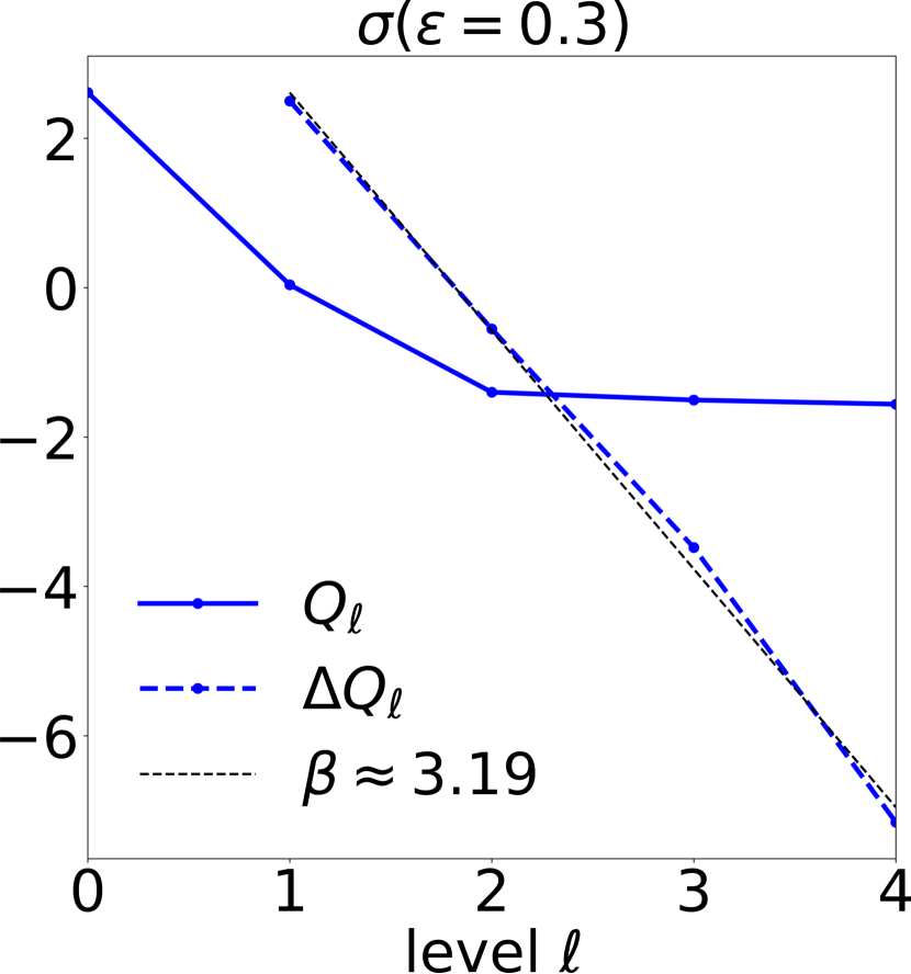
(c) $\displaystyle\varepsilon=0.30$

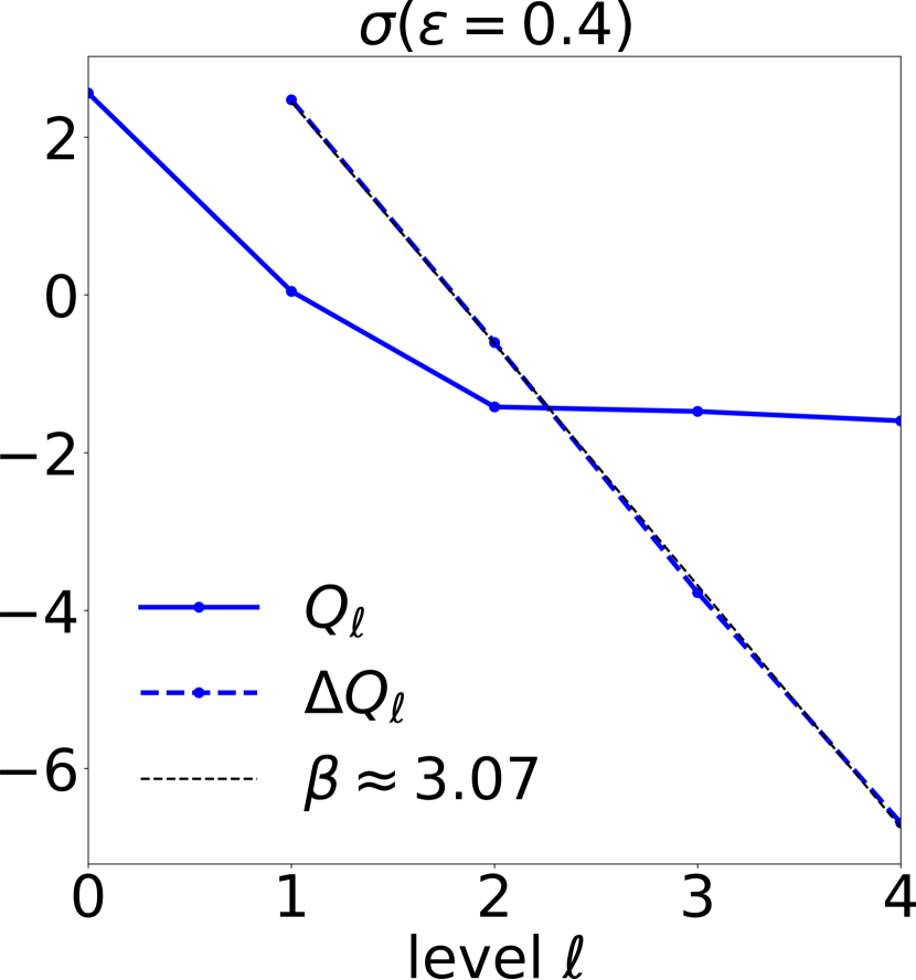
(d) $\displaystyle\varepsilon=0.40$

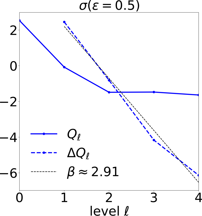
(e) $\displaystyle\varepsilon=0.50$

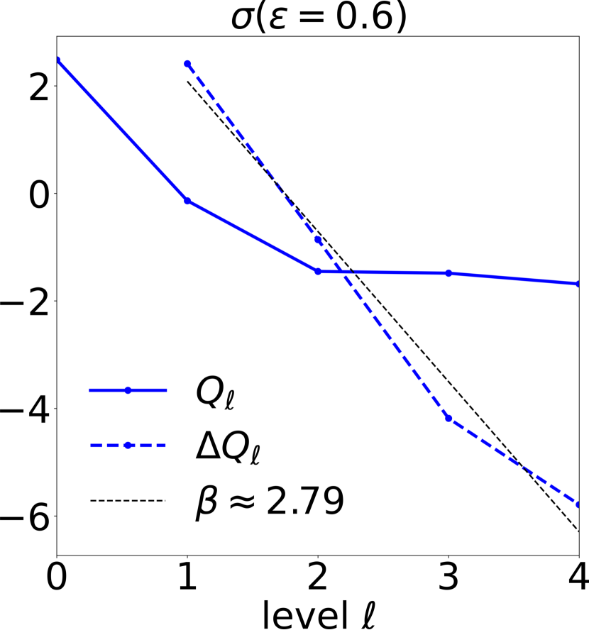
(f) $\displaystyle\varepsilon=0.60$

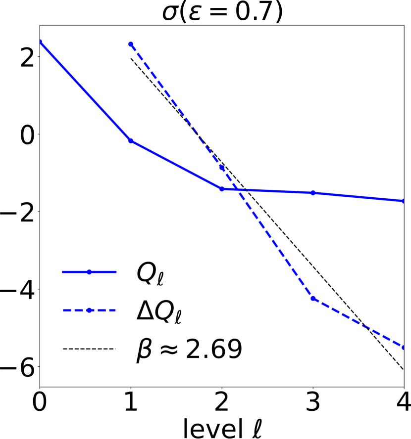
(g) $\displaystyle\varepsilon=0.70$

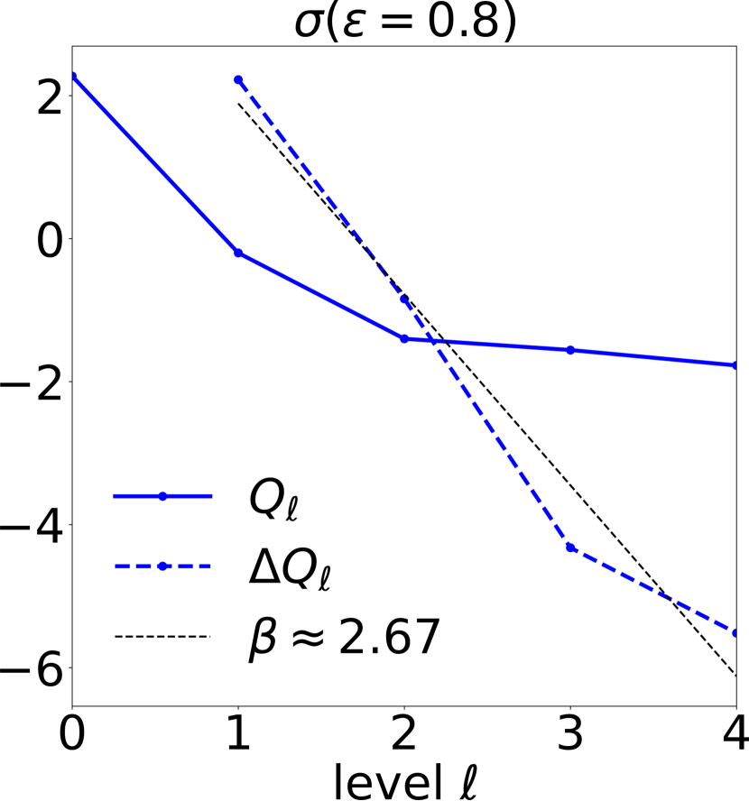
(h) $\displaystyle\varepsilon=0.80$

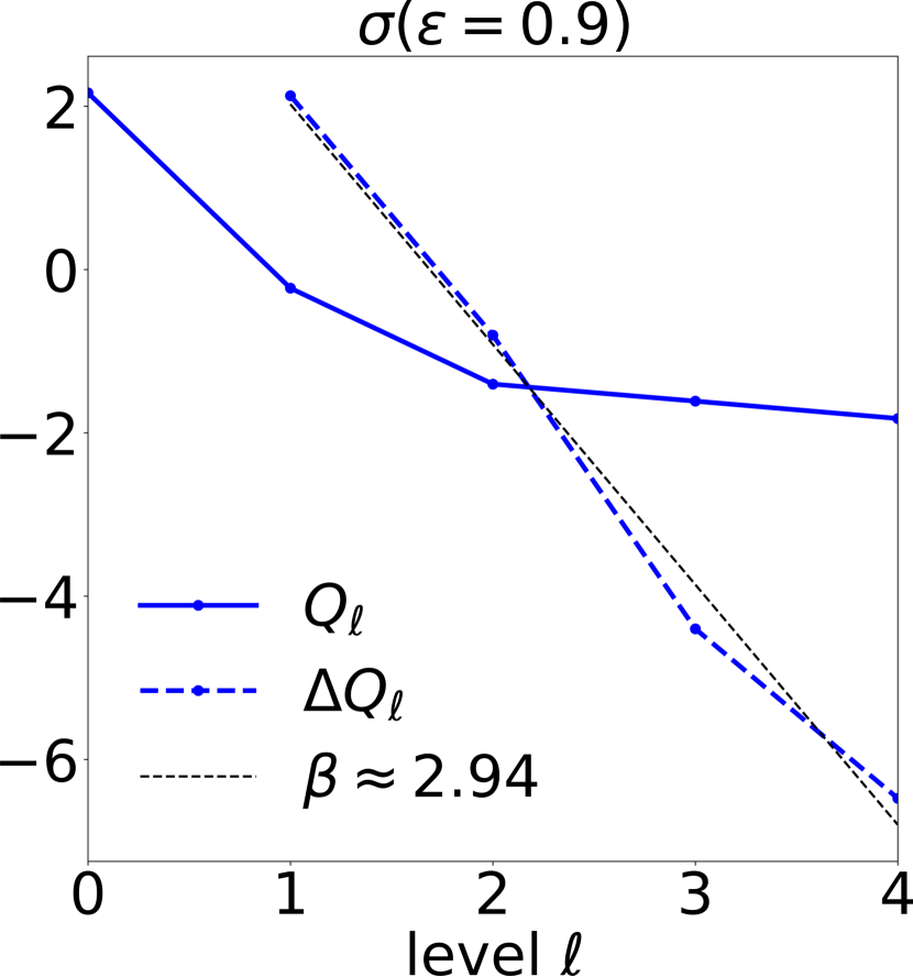
(i) $\displaystyle\varepsilon=0.90$

Figure 7: Behavior of the variance $\displaystyle\log_{2}(\mathbb{V}[\left|\cdot\right|])$ of the QoI $\displaystyle Q_{\ell}$ and the multi-level difference $\displaystyle\Delta Q_{\ell}$ as a function of the level $\displaystyle\ell$ using the mesh refinement as a fidelity parameter for each QoI. We numerically fitted the values $\displaystyle{\mathbb{V}}[\Delta Q_{\ell}]\;\propto\;2^{-\beta\ell}$ with $\displaystyle 2.62\lesssim\beta\lesssim 3.53$, see Table 3.

The behavior of the expected value of the QoIs $\displaystyle Q_{\ell}$ and the multilevel difference $\displaystyle Q_{\ell}-Q_{\ell-1}$ is shown in Figure 6. The expected value $\displaystyle{\mathbb{E}\left[Q_{\ell}\right]}$ is stable across all levels $\displaystyle\ell=0,1,\ldots,4$, and the expected value of the multilevel difference decays as the mesh resolution level $\displaystyle\ell$ increases. Table 3 shows the numerically fitted decay rates $\displaystyle\alpha$ from condition (C1).

The behavior of the variance of the QoIs $\displaystyle Q_{\ell}$ and the multilevel difference $\displaystyle Q_{\ell}-Q_{\ell-1}$ is shown in Figure 7. As shown in Figure 5, the most materials variability comes from $\displaystyle 2\times 2\times 2$, and the least materials variability comes from $\displaystyle 32\times 32\times 32$, possibly due to the number of grains in SERVEs. This observation is consistent with the quantitative analysis of variance shown in Figure 7. For mesh resolution levels 1 and 2 the variance of the multilevel difference $\displaystyle{\mathbb{V}\left[\Delta Q_{\ell}\right]}$, is more than the variance of the quantity of interest $\displaystyle{\mathbb{V}\left[Q_{\ell}\right]}$ itself, i.e. $\displaystyle{\mathbb{V}\left[\Delta Q_{\ell}\right]}>{\mathbb{V}\left[Q_{\ell}\right]}$ with $\displaystyle\ell=1,2$. This means that the necessary condition for an efficient MLMC estimator required in (12) is not satisfied (note the logarithmic axis for the variance). A lack of correlation between the QoIs derived from microstructures at levels $\displaystyle\ell=$ 0, 1, and 2 explains this constraint violation, see Figure 2 for an illustration. However, the variance of the multilevel difference does satisfy condition (C2) with numerically fitted rates $\displaystyle\beta$ shown in Table 3. In order to ensure that our MLMC estimator is efficient, we remove the first three levels in the multilevel hierarchy, leaving only mesh resolution levels $\displaystyle\ell=3$ and $\displaystyle\ell=4$. Since $\displaystyle 2\alpha\geq\min(\beta,\gamma)$ for all QoIs, we expect an asymptotic cost complexity of $\displaystyle\mathcal{O}(\epsilon^{-2})$, see (16).

It is observed that the expectation across all fidelity levels $\displaystyle\ell$ is stable (Figure 6), whereas the variance across all fidelity levels $\displaystyle\ell$, while generally still decreasing, is only useful when $\displaystyle\ell\geq 3$. We postulate that the convergence of the expectation has more to do with the underlying constitutive models, whereas the variance has more to do with the number of grains in SERVEs. The converged expectation is consistent in the notion of unbiased estimator (for both MLMC and MC methods, as any MC-based approach is naturally unbiased), but the variance depends on number of SERVEs $\displaystyle N$ (Equation (4)), and implicitly the number of grains. In this sense, there may be a meaningful criteria to establish a bound for low-fidelity representation of SERVEs, so that the correlation constraint in Equation (12) can be satisfied.

Table 3: Fitted decay rates $\displaystyle\alpha$ and $\displaystyle\beta$ in conditions (C1) and (C2), respectively.

$\displaystyle\varepsilon$	$\displaystyle\alpha$	$\displaystyle\beta$
0.1	2.93	3.53
0.2	2.26	3.44
0.3	2.64	3.15
0.4	1.59	3.02
0.5	1.30	2.88
0.6	1.19	2.76
0.7	1.16	2.64
0.8	1.25	2.62
0.9	1.56	2.93

4.3 Comparison between MC and MLMC

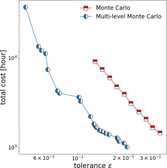
Figure 8: Total cost comparison between MC and MLMC showing a factor of around 2.23$\displaystyle\times$ speedup.

In Figure 8, we show a comparison of the computational cost, measured in wall clock time, of the MC and MLMC methods, for different values of the tolerance parameter $\displaystyle\epsilon$. The MLMC method outperforms the MC method by a factor of 2.23$\displaystyle\times$. For a tolerance $\displaystyle\epsilon=1.30e-1$, the plain MC method takes 1283.38 hours, while our MLMC method takes approximately 68.14 hours. Table 4 tabulates the comparison between MLMC and MC methods, where the number of SERVEs at level $\displaystyle\ell=4$, $\displaystyle N_{4}$, in the MC method is approximated by $\displaystyle N_{3}$ in the MLMC method. The reasoning behind this approximation is that we assume the variance on the low-fidelity (coarse) level, i.e. $\displaystyle\ell=3$ is approximately the same with the high-fidelity (fine) level, i.e. $\displaystyle\ell=4$. The approximately same variance means approximately the same number of samples, and therefore, the number of SERVEs $\displaystyle N_{4}$ in the MC method can be approximated by $\displaystyle N_{3}$ in the MLMC method. Because MF UQ methods generally aim to argue that it is possible to conduct UQ efficiently by multiple levels of fidelity, the best way to highlight the efficiency is simply to compare the MF UQ method at hand with the brute-force high-fidelity counterpart. Therefore, we only consider an approximate $\displaystyle N_{4}$ and not $\displaystyle N_{3}$ for the MC method.

Table 4: Comparison of the distribution of the number of samples across the mesh resolution levels for MLMC and MC, for different tolerances $\displaystyle\epsilon$.

$\displaystyle\epsilon$	MC		MLMC			Speedup
	Approx. $\displaystyle N_{4}$	Approx. Cost (hr)	$\displaystyle N_{3}$	$\displaystyle N_{4}$	Cost (hr)
3.51000000e-01	7	24.28	7	3	16.83	1.44$\displaystyle\times$
3.14324193e-01	8	27.74	8	3	17.75	1.56$\displaystyle\times$
2.81480622e-01	10	34.68	10	3	19.58	1.77$\displaystyle\times$
2.52068859e-01	12	41.62	12	3	21.42	1.94$\displaystyle\times$
2.25730315e-01	15	52.02	15	3	24.17	2.15$\displaystyle\times$
2.02143872e-01	19	65.90	19	3	27.84	2.36$\displaystyle\times$
1.81021965e-01	23	79.77	23	3	31.52	2.53$\displaystyle\times$
1.62107074e-01	29	100.58	29	3	37.02	2.71$\displaystyle\times$
1.45168590e-01	36	124.87	36	4	46.92	2.66$\displaystyle\times$
1.30000000e-01	44	152.61	44	8	68.14	2.23$\displaystyle\times$

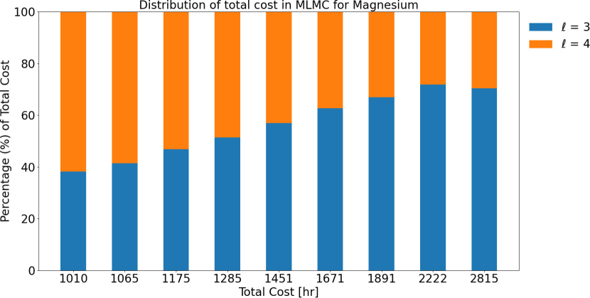
Figure 9: Total cost distribution for MLMC run with only levels $\displaystyle\ell=3,4$ showing an increase of computational resource allocation toward the low-fidelity level as the total cost increases.

In Figure 9 we show the distribution of the total cost among the levels, measured as a percentage of the wall clock time, as a function of the total cost. As the total cost increases, more and more time is spent evaluating the QoIs using a coarse mesh resolution level. For a total cost over 2000 hours, only a quarter of the time is spent evaluating the QoIs at the finest resolution level.

5 Discussion

The novelty of this paper lies in the integration of the methodology (i.e. MLMC) and the application (CPFEM) by approaching the classical problem in CPFEM at a different UQ perspective, but not the methodology or the application itself. Given that the interest in UQ for materials science has emerged in the last few years and the ensemble of SERVEs has been the main approach for the last two decades or so, it is non-trivial to formulate the UQ problem through the correct lens, where the right methodology is married to the right application.

Several techniques that exploit a hierarchy of model approximations have been introduced in the recent literature. The multi-index Monte Carlo (MIMC) haji2016multi method, for example, uses a multi-dimensional hierarchy to further increase the efficiency. This multi-dimensional hierarchy may include refinement levels such as constitutive models, integration time-step, or $\displaystyle hp$-FEM, where $\displaystyle h$ corresponds to mesh size and $\displaystyle p$ corresponds to polynomial degree of the finite element. In our previous work in tran2023multi we applied MIMC for a single-QoI CPFEM application. For non-hierarchical model approximations, we mention multi-fidelity MC (MFMC) peherstorfer2016optimal ; peherstorfer2018survey ; qian2018multifidelity and approximate control variates gorodetsky2020generalized ; schaden2020multilevel ; schaden2021asymptotic ; bomarito2022optimization .

The analysis of the variance in Figure 7 shows that there is a limitation to the amount of mesh coarsening we can perform in order to yield an efficient multilevel estimator. When the mesh resolution becomes too coarse, the QoIs extracted from the discretized microstructures are no longer correlated, a necessary requirement for a good control variate as per equation (12). Such behavior can only be observed through a preliminary analysis of the problem, such as the one performed in this paper. In order to improve the correlation between microstructure resolutions at intermediate mesh resolution levels, the element agglomeration technique from the algebraic multigrid literature may be useful.

There is a lower bound for low-fidelity levels (so that Equation (12) is not violated), but there is no upper bound for high-fidelity levels. The MLMC method is at most much better and at least on par with the MC method. The equality in terms of performance occurs when there is only one level of fidelity, as the MLMC method is a natural MF extension of the MC method.

One important limitation of the MLMC methods is that it requires a substantial correlation across multiple fidelity levels (i.e. $\displaystyle Q_{\ell}$ and $\displaystyle Q_{\ell-1}$ in (12)). Without sufficient correlation, the variance $\displaystyle{\mathbb{V}\left[\Delta Q_{\ell}\right]}$ will not be substantially reduced, and thus the gain of using MLMC methods would be marginal compared to MC methods.

The generalization of MLMC methods for CPFEM in various materials system is clear, where it can be applied to various materials systems of interests. The MLMC method is a generic framework for MF UQ problems, with the objective of quantifying the uncertainty by leveraging a multi-fidelity hierarchy. There are several mathematical restrictions, such as strong correlation (12) and exponential decay in expectation, variance, and computational cost, i.e. (C1), (C2), and (C3). The exponential decay assumptions, in general, are naturally satisfied as long as the CPFEM converges at all levels $\displaystyle\ell$’s. Perhaps, it is worthy to note that in this work, we focus solely on the case of 1-dimension in fidelity parameters (i.e. mesh resolutions) and multi objectives (i.e. stress observations at 9 collocated points), while in previous work tran2023multi , we focused on multi-dimension in fidelity parameters (i.e. mesh resolutions and constitutive models) with single objective (i.e. Young modulus or yield strength).

It is well-known that there is a close relationship between the materials texture characterized by the orientation distribution functions and the materials stress-strain response. In this work, we follow Mangal and Holm mangal2018dataset to study the texture of magnesium with $\displaystyle(\phi_{1},\theta,\phi_{2})=(90^{\circ},0^{\circ},0^{\circ})$ as an exemplar for our proposed UQ problem. How material textures influence the material stress-strain responses is certainly a very interesting question, but it lies beyond the scope of this paper, and therefore, is an subject of interest for future study.

Finally, we point out that the CPFEM method, just as all other finite-element-based method, introduces several layers of approximation errors. A first error occurs because of the discretization of the geometry. A second source of error is the accuracy of the sparse linear solver used to compute the finite element solutions. In this work, we have focused on the former error, but it possible to include the solver accuracy as an additional dimension for refinement, possibly in a multi-index Monte Carlo framework.

6 Conclusion

In this paper, we applied the MLMC method to study the effect of microstructure variation on the stress-strain curves for magnesium predicted by CPFEM. We imposed a geometric mesh hierarchy with five different mesh resolution levels, of which only the two finest levels were used in an efficient multilevel sampling strategy. Our MLMC method outperforms the standard MC method by a factor of 2.23$\displaystyle\times$.

References

- \bibcommenthead
- (1) G.B. Olson, Computational design of hierarchically structured materials. Science 277(5330), 1237–1242 (1997)
- (2) R. Arróyave, D.L. McDowell, Systems approaches to materials design: Past, present, and future. Annual Review of Materials Research 49(1), 103–126 (2019)
- (3) T. Hey, S. Tansley, K.M. Tolle, The fourth paradigm: data-intensive scientific discovery, vol. 1 (Microsoft research Redmond, WA, 2009)
- (4) A. Agrawal, A. Choudhary, Perspective: Materials informatics and big data: Realization of the “fourth paradigm” of science in materials science. APL Materials 4(5), 053,208 (2016)
- (5) U.N.R. Council, Integrated computational materials engineering: a transformational discipline for improved competitiveness and national security (National Academies Press, 2008)
- (6) US NSTC, Materials Genome Initiative for global competitiveness (Executive Office of the President, National Science and Technology Council, 2011)
- (7) J.J. de Pablo, N.E. Jackson, M.A. Webb, L.Q. Chen, J.E. Moore, D. Morgan, R. Jacobs, T. Pollock, D.G. Schlom, E.S. Toberer, J. Analytis, I. Dabo, D.M. DeLongchamp, G.A. Fiete, G.M. Grason, G. Hautier, Y. Mo, K. Rajan, E.J. Reed, E. Rodriguez, V. Stevanovic, J. Suntivich, K. Thornton, J.C. Zhao, New frontiers for the materials genome initiative. npj Computational Materials 5(1), 1–23 (2019)
- (8) T. Oden, R. Moser, O. Ghattas, Computer predictions with quantified uncertainty, Part I. SIAM News 43(9), 1–3 (2010)
- (9) T. Oden, R. Moser, O. Ghattas, Computer predictions with quantified uncertainty, Part II. SIAM News 43(10), 1–4 (2010)
- (10) T. Nguyen, D.C. Francom, D.J. Luscher, J. Wilkerson, Bayesian calibration of a physics-based crystal plasticity and damage model. Journal of the Mechanics and Physics of Solids 149, 104,284 (2021)
- (11) M. Hasan, P. Acar, Microstructure-sensitive stochastic design of polycrystalline materials for quasi-isotropic properties. AIAA Journal 60(12), 6869–6880 (2022)
- (12) A. Tran, D. Liu, H.A. Tran, Y. Wang, Quantifying uncertainty in the process-structure relationship for Al-Cu solidification. Modelling and Simulation in Materials Science and Engineering 27(6), 064,005 (2019)
- (13) A. Tran, T. Wildey, H. Lim, Microstructure-sensitive uncertainty quantification for crystal plasticity finite element constitutive models using stochastic collocation method. Frontiers in Materials 9, 1–20 (2022)
- (14) A. Venkatraman, S. Mohan, R. Joseph, D.L. McDowell, S.R. Kalidindi, A new framework for the assessment of model probabilities of the different crystal plasticity models for lamellar grains in + Titanium alloys. Modelling and Simulation in Materials Science and Engineering (2023)
- (15) M. Rixner, P.S. Koutsourelakis, Self-supervised optimization of random material microstructures in the small-data regime. npj Computational Materials 8(1), 46 (2022)
- (16) A. Tran, T. Wildey, Solving stochastic inverse problems for property-structure linkages using data-consistent inversion and machine learning. JOM 73, 72–89 (2020)
- (17) T. Butler, J. Jakeman, T. Wildey, Combining push-forward measures and Bayes’ rule to construct consistent solutions to stochastic inverse problems. SIAM Journal on Scientific Computing 40(2), A984–A1011 (2018)
- (18) T. Butler, J. Jakeman, T. Wildey, Convergence of probability densities using approximate models for forward and inverse problems in uncertainty quantification. SIAM Journal on Scientific Computing 40(5), A3523–A3548 (2018)
- (19) A. Tran, P. Robbe, H. Lim, Multi-fidelity microstructure-induced uncertainty quantification by advanced monte carlo methods. Materialia 27, 101,705 (2023)
- (20) T.M. Rodgers, H. Lim, J.A. Brown, Three-dimensional additively manufactured microstructures and their mechanical properties. JOM 72(1), 75–82 (2020)
- (21) J.A. Mitchell, F. Abdeljawad, C. Battaile, C. Garcia-Cardona, E.A. Holm, E.R. Homer, J. Madison, T.M. Rodgers, A.P. Thompson, V. Tikare, E. Webb, S.J. Plimpton, Parallel simulation via SPPARKS of on-lattice kinetic and Metropolis Monte Carlo models for materials processing. Modelling and Simulation in Materials Science and Engineering 31(5), 055,001 (2023)
- (22) A. Tran, H. Lim, An asynchronous parallel high-throughput model calibration framework for crystal plasticity finite element constitutive models. Computational Mechanics (2023)
- (23) A. Tran, M. Eldred, T. Wildey, S. McCann, J. Sun, R.J. Visintainer, aphBO-2GP-3B: a budgeted asynchronous parallel multi-acquisition functions for constrained Bayesian optimization on high-performing computing architecture. Structural and Multidisciplinary Optimization 65(4), 1–45 (2022)
- (24) D.E. Ricciardi, O.A. Chkrebtii, S.R. Niezgoda, Uncertainty quantification accounting for model discrepancy within a random effects bayesian framework. Integrating Materials and Manufacturing Innovation 9, 181–198 (2020)
- (25) M.C. Kennedy, A. O’Hagan, Bayesian calibration of computer models. Journal of the Royal Statistical Society: Series B (Statistical Methodology) 63(3), 425–464 (2001)
- (26) M. Khalil, G.H. Teichert, C. Alleman, N. Heckman, R.E. Jones, K. Garikipati, B. Boyce, Modeling strength and failure variability due to porosity in additively manufactured metals. Computer Methods in Applied Mechanics and Engineering 373, 113,471 (2021)
- (27) S.F. Ghoreishi, A. Molkeri, A. Srivastava, R. Arroyave, D. Allaire, Multi-information source fusion and optimization to realize ICME: Application to dual-phase materials. Journal of Mechanical Design 140(11), 111,409 (2018)
- (28) M. Groeber, S. Ghosh, M.D. Uchic, D.M. Dimiduk, A framework for automated analysis and simulation of 3D polycrystalline microstructures. Part 1: Statistical characterization. Acta Materialia 56(6), 1257–1273 (2008)
- (29) M. Groeber, S. Ghosh, M.D. Uchic, D.M. Dimiduk, A framework for automated analysis and simulation of 3D polycrystalline microstructures. Part 2: Synthetic structure generation. Acta Materialia 56(6), 1274–1287 (2008)
- (30) S. Torquato, Statistical description of microstructures. Annual review of materials research 32(1), 77–111 (2002)
- (31) R. Bostanabad, Y. Zhang, X. Li, T. Kearney, L.C. Brinson, D.W. Apley, W.K. Liu, W. Chen, Computational microstructure characterization and reconstruction: Review of the state-of-the-art techniques. Progress in Materials Science 95, 1–41 (2018)
- (32) N.H. Paulson, M.W. Priddy, D.L. McDowell, S.R. Kalidindi, Reduced-order structure-property linkages for polycrystalline microstructures based on 2-point statistics. Acta Materialia 129, 428–438 (2017)
- (33) K. Teferra, L. Graham-Brady, A random field-based method to estimate convergence of apparent properties in computational homogenization. Computer Methods in Applied Mechanics and Engineering 330, 253–270 (2018)
- (34) N.H. Paulson, M.W. Priddy, D.L. McDowell, S.R. Kalidindi, Data-driven reduced-order models for rank-ordering the high cycle fatigue performance of polycrystalline microstructures. Materials & Design 154, 170–183 (2018)
- (35) C. Robert, G. Casella, Monte Carlo statistical methods (Springer Science & Business Media, 2013)
- (36) I. Babuška, M. Suri, The and versions of the finite element method, an overview. Computer methods in applied mechanics and engineering 80(1-3), 5–26 (1990)
- (37) M.B. Giles, Multilevel Monte Carlo methods. Acta Numerica 24, 259–328 (2015)
- (38) K.A. Cliffe, M.B. Giles, R. Scheichl, A.L. Teckentrup, Multilevel monte carlo methods and applications to elliptic pdes with random coefficients. Computing and Visualization in Science 14(1), 3–15 (2011)
- (39) P. Robbe, D. Nuyens, S. Vandewalle, A multi-index quasi–monte carlo algorithm for lognormal diffusion problems. SIAM Journal on Scientific Computing 39(5), S851–S872 (2017)
- (40) P. Robbe, D. Nuyens, S. Vandewalle, Recycling samples in the multigrid multilevel (quasi-) Monte Carlo method. SIAM Journal on Scientific Computing 41(5), S37–S60 (2019)
- (41) M.A. Groeber, M.A. Jackson, DREAM.3D: a digital representation environment for the analysis of microstructure in 3D. Integrating materials and manufacturing innovation 3(1), 5 (2014)
- (42) F. Roters, M. Diehl, P. Shanthraj, P. Eisenlohr, C. Reuber, S. Wong, T. Maiti, A. Ebrahimi, T. Hochrainer, H.O. Fabritius, S. Nikolov, M. Friák, N. Fujita, N. Grilli, K. Janssens, N. Jia, P. Kok, D. Ma, F. Meier, E. Werner, M. Stricker, D. Weygand, D. Raabe, DAMASK–The Düsseldorf Advanced Material Simulation Kit for modeling multi-physics crystal plasticity, thermal, and damage phenomena from the single crystal up to the component scale. Computational Materials Science 158, 420–478 (2019)
- (43) S. Balay, W.D. Gropp, L.C. McInnes, B.F. Smith, in Modern software tools for scientific computing (Springer, 1997), pp. 163–202
- (44) S. Balay, S. Abhyankar, M.F. Adams, S. Benson, J. Brown, P. Brune, K. Buschelman, E.M. Constantinescu, L. Dalcin, A. Dener, V. Eijkhout, J. Faibussowitsch, W.D. Gropp, V. Hapla, T. Isaac, P. Jolivet, D. Karpeev, D. Kaushik, M.G. Knepley, F. Kong, S. Kruger, D.A. May, L.C. McInnes, R.T. Mills, L. Mitchell, T. Munson, J.E. Roman, K. Rupp, P. Sanan, J. Sarich, B.F. Smith, S. Zampini, H. Zhang, H. Zhang, J. Zhang. PETSc Web page. https://petsc.org/ (2023). URL https://petsc.org/
- (45) F. Roters, P. Eisenlohr, L. Hantcherli, D.D. Tjahjanto, T.R. Bieler, D. Raabe, Overview of constitutive laws, kinematics, homogenization and multiscale methods in crystal plasticity finite-element modeling: Theory, experiments, applications. Acta Materialia 58(4), 1152–1211 (2010)
- (46) F. Roters, P. Eisenlohr, T.R. Bieler, D. Raabe, Crystal plasticity finite element methods: in materials science and engineering (John Wiley & Sons, 2011)
- (47) K. Sedighiani, M. Diehl, K. Traka, F. Roters, J. Sietsma, D. Raabe, An efficient and robust approach to determine material parameters of crystal plasticity constitutive laws from macro-scale stress–strain curves. International Journal of Plasticity 134, 102,779 (2020)
- (48) K. Sedighiani, K. Traka, F. Roters, D. Raabe, J. Sietsma, M. Diehl, Determination and analysis of the constitutive parameters of temperature-dependent dislocation-density-based crystal plasticity models. Mechanics of Materials 164, 104,117 (2022)
- (49) F. Wang, S. Sandlöbes, M. Diehl, L. Sharma, F. Roters, D. Raabe, In situ observation of collective grain-scale mechanics in Mg and Mg–rare earth alloys. Acta materialia 80, 77–93 (2014)
- (50) D. Tromans, Elastic anisotropy of HCP metal crystals and polycrystals. Int. J. Res. Rev. Appl. Sci 6(4), 462–483 (2011)
- (51) S. Agnew, D. Brown, C. Tomé, Validating a polycrystal model for the elastoplastic response of magnesium alloy AZ31 using in situ neutron diffraction. Acta materialia 54(18), 4841–4852 (2006)
- (52) A. Mangal, E.A. Holm, A dataset of synthetic hexagonal close packed 3d polycrystalline microstructures, grain-wise microstructural descriptors and grain averaged stress fields under uniaxial tensile deformation for two sets of constitutive parameters. Data in brief 21, 1833–1841 (2018)
- (53) P. Virtanen, R. Gommers, T.E. Oliphant, M. Haberland, T. Reddy, D. Cournapeau, E. Burovski, P. Peterson, W. Weckesser, J. Bright, S.J. van der Walt, M. Brett, J. Wilson, K.J. Millman, N. Mayorov, A.R.J. Nelson, E. Jones, R. Kern, E. Larson, C.J. Carey, I. Polat, Y. Feng, E.W. Moore, J. VanderPlas, D. Laxalde, J. Perktold, R. Cimrman, I. Henriksen, E.A. Quintero, C.R. Harris, A.M. Archibald, A.H. Ribeiro, F. Pedregosa, P. van Mulbregt, A. Vijaykumar, A.P. Bardelli, A. Rothberg, A. Hilboll, A. Kloeckner, A. Scopatz, A. Lee, A. Rokem, C.N. Woods, C. Fulton, C. Masson, C. Häggström, C. Fitzgerald, D.A. Nicholson, D.R. Hagen, D.V. Pasechnik, E. Olivetti, E. Martin, E. Wieser, F. Silva, F. Lenders, F. Wilhelm, G. Young, G.A. Price, G.L. Ingold, G.E. Allen, G.R. Lee, H. Audren, I. Probst, J.P. Dietrich, J. Silterra, J.T. Webber, J. Slavič, J. Nothman, J. Buchner, J. Kulick, J.L. Schönberger, J.V. de Miranda Cardoso, J. Reimer, J. Harrington, J.L.C. Rodríguez, J. Nunez-Iglesias, J. Kuczynski, K. Tritz, M. Thoma, M. Newville, M. Kümmerer, M. Bolingbroke, M. Tartre, M. Pak, N.J. Smith, N. Nowaczyk, N. Shebanov, O. Pavlyk, P.A. Brodtkorb, P. Lee, R.T. McGibbon, R. Feldbauer, S. Lewis, S. Tygier, S. Sievert, S. Vigna, S. Peterson, S. More, T. Pudlik, T. Oshima, T.J. Pingel, T.P. Robitaille, T. Spura, T.R. Jones, T. Cera, T. Leslie, T. Zito, T. Krauss, U. Upadhyay, Y.O. Halchenko, Y. Vázquez-Baeza, SciPy 1.0 Contributors, SciPy 1.0: fundamental algorithms for scientific computing in Python. Nature methods 17(3), 261–272 (2020)
- (54) A.L. Haji-Ali, F. Nobile, R. Tempone, Multi-index Monte Carlo: when sparsity meets sampling. Numerische Mathematik 132(4), 767–806 (2016)
- (55) B. Peherstorfer, K. Willcox, M. Gunzburger, Optimal model management for multifidelity Monte Carlo estimation. SIAM Journal on Scientific Computing 38(5), A3163–A3194 (2016)
- (56) B. Peherstorfer, K. Willcox, M. Gunzburger, Survey of multifidelity methods in uncertainty propagation, inference, and optimization. SIAM Review 60(3), 550–591 (2018)
- (57) E. Qian, B. Peherstorfer, D. O’Malley, V.V. Vesselinov, K. Willcox, Multifidelity Monte Carlo estimation of variance and sensitivity indices. SIAM/ASA Journal on Uncertainty Quantification 6(2), 683–706 (2018)
- (58) A.A. Gorodetsky, G. Geraci, M.S. Eldred, J.D. Jakeman, A generalized approximate control variate framework for multifidelity uncertainty quantification. Journal of Computational Physics 408, 109,257 (2020)
- (59) D. Schaden, E. Ullmann, On multilevel best linear unbiased estimators. SIAM/ASA Journal on Uncertainty Quantification 8(2), 601–635 (2020)
- (60) D. Schaden, E. Ullmann, Asymptotic analysis of multilevel best linear unbiased estimators. SIAM/ASA Journal on Uncertainty Quantification 9(3), 953–978 (2021)
- (61) G.F. Bomarito, P.E. Leser, J.E. Warner, W.P. Leser, On the optimization of approximate control variates with parametrically defined estimators. Journal of Computational Physics 451, 110,882 (2022)